The Traveling Wave Loop Antenna: A Terminated Wire Loop Aerial for Directional High-Frequency Ocean RADAR Transmission

Abstract

In this paper we document the design, development, results, performance and field applications of a compact directive transmit antenna for the long-range High Frequency ocean RADAR (HFR) systems operating in the International Telecommunication Union (ITU) designated $4\mathrm{MHz}$ and $5\mathrm{MHz}$ radiodetermination bands. The antenna design is based on the combination of the concepts of an electrically small loop with that of travelling wave antenna. This has the effect of inducing a radiated wave predominantly in a direction opposed to that of energy flow on the antenna structures. We demonstrate here that travelling wave design allows for a more compact antenna than other directive options, it has straightforward feed-point matching arrangements, and a flat frequency and phase response over an entire radiodetermination band. In situ measurements of the antenna radiation pattern, obtained with the aid of a drone, correlate well with those obtained from simulations, and show between $8\mathrm{dB}$ and $30\mathrm{dB}$ front-to-back suppression, with a $3\mathrm{dB}$ beam width in the forward lobe of ${100}^{\circ }$ or more. The broad-beam radiation pattern ensures proper illumination over the ocean and the significant front-to-back suppression guarantees reduced interference to terrestrial services. The proposed antenna design is compact and straight forward and can be easily deployed by minimal modifications of an existing transmission antenna. The design may be readily adapted to different environments due to the relative insensitivity of its radiation pattern and frequency response to geometric detail. The only downside to these antennas is their relatively low radiation efficiency which, however, may easily be compensated for by the available power output of a typical HFR transmitter. Antennas based on this design are currently deployed at the SeaSonde HFR sites in New South Wales, Australia, with operational ranges up to 200 km offshore despite their low radiating efficiency and the extremely low output power in use at these installations. Due to their directional pattern, it is also planned to test these antennas in phased-array Wellen RADAR (WERA) systems in both the standard receive arrays: where in-band radio frequency noise of terrestrial origin is impacting on data quality, and in the transmit array: to possibly simplify splitting, phasing and tuning requirements.

1. Introduction

High Frequency RADAR (HFR) measurements of surface currents in the coastal ocean have become a standard and cost-effective component for ocean observing systems globally [1,2,3]. Developed more than four decades ago [4], oceanographic HFR provides highly accurate synoptic observation of large scale coastal circulation features at high temporal and spatial resolutions not readily obtained using conventional instrumentation [5,6]. HFRs now constitute a fundamental component of coastal observing networks, due to: their utility in understanding processes such as air-sea interaction, coastal circulation and tidal flows; their ability to support search and rescue operations, and the direction toxic-spill mitigation activities; and as tsunami early-warning systems [1,2,3].

HFR systems rely on the backscatter of vertically polarized electromagnetic energy in the 3–50 MHz frequency range to observe the sea surface state. Results are obtained on the basis of the Bragg scatter mechanism and Doppler shift of the first-order Bragg spectral lines [2,4,7]. An individual HFR system operated in a conventional monostatic configuration maps the depth-integrated component of an ocean current advancing towards or receding from its associated receiver [4]. Depending on the operating frequency, this measurement is representative of the top 0.5–2.5 m layer of the ocean [8]. Multifrequency HFR systems, such as for instance [9,10,11,12], therefore allow for the vertical resolution of the velocity profile within a water column. Two or more HFRs overlooking the same patch of ocean from different locations are required to resolve the two-dimensional current field in the area of common overlap.

Based on the approach used to resolve the azimuth of the first-order Bragg spectral lines, oceanographic HFR systems may be broadly classified as direction-finding or beam-forming systems. Direction-Finding, as implemented commercially by SeaSonde [13] and similar systems developed at Wuhan University [9,14], employ directional antennas with differing orientations and the principals of Radio Direction Finding (RDF). Beam-forming, as per the commercially available Wellen RADAR (WERA) systems [15], similar systems developed by the University of Hawaii [16,17], and PISCES [18], employ an array of similar receiving antennas and combine their output to focus attention on reflected signals originating from a predefined grid cell. Performance, advantages and disadvantages of the two approaches have been discussed extensively elsewhere (for instance, [19,20]), and will not be discussed further as they are outside the scope of the present paper.

Regardless of the approach to the azimuthal resolution in the receiver, most oceanographic HFR systems commonly utilise a wide-beam “floodlight” transmission to “illuminate” an entire coastal ocean region of interest. This illumination may be accomplished with either an omnidirectional antenna (SeaSonde and similar systems) or broadly directional antenna array (WERA and similar systems). A third type of oceanographic RADAR system exists for the Very High Frequency (VHF) band, where reduced wavelength and consequently antenna dimensions, allow the combination of narrow-beam synthetic aperture arrays for both directive transmission and reception on a common steerable antenna, resulting in improved sensitivity [21].

Other types of RADAR systems exist and operate well into the microwave “X-Band” region. These extremely short wavelengths allow the use of the highly directional and extremely compact rotatable antennas on which the operation of these systems rely. These antennas consist of a large number of phased slot or stripline antenna arrays. These systems exist at the opposite end of the radio spectrum where physical size of multi-wavelength structures is not a limiting factor in deployment. Examples of applications may be found in [22].

In general, direction-finding systems tend to be more compact than their beam-forming counterparts, largely due to the use of the more compact co-located receiving antennas. A gated transmission signal, namely Frequency Modulated Interrupted Continuous Wave (FMICW), allows for the further co-location of the transmit and receive antennas on a single mast. In contrast, beam-forming systems typically use a distributed receive array extending over several wavelengths and utilise a separate directional transmit array. This physical separation and directionality are necessary to prevent saturation of the receivers by the uninterrupted transmitted signal.

Broad-beam directionality in the transmit pattern is clearly an advantage for both types of HFR systems to minimise unwanted transmission over land and to ensure that the coastal ocean is illuminated as uniformly as possible. However, directionality often comes to the detriment of antenna dimension, complexity, and the overall land-area required for deployment. In general antenna dimensions and spacings vary in proportion to wavelength, $\lambda {}_{f_c}^{}$, and consequently the area taken up by ${\left(\lambda {}_{f_c}^{}\right)}^2$. In the $4\mathrm{MHz}$ and $5\mathrm{MHz}$ allocations, the dimension and spacing of the transmit antennas become a limiting factor in relation to the development of directive arrays.

In the long-range ($4\mathrm{MHz}$ and $5\mathrm{MHz}$) HFR bands, SeaSonde systems use an approximately 9 m tall bottom-fed, center loaded element with/without a capacitive top-hat, resulting in a physically short vertical element (<0.25$\lambda {}_{f_c}^{}$) with an electrical resonance in combination with the grounding system corresponding to $0.5\lambda {}_{f_c}^{}$ [23]. The SeaSonde loading coil consists of two sections $L_1\approx 15\mathsf{\mu }\mathrm{H}$ and $L_2\approx 34\mathsf{\mu }\mathrm{H}$. The coil $L_1$ may be bypassed with a shorting strap to assist in providing a better match. This is adjusted at installation as required. A capacitive top hat may be similarly installed but is generally only required on the $4\mathrm{MHz}$ band.

A single-element vertical antenna is typically characterised by an omnidirectional radiation pattern. Directivity may be achieved through deployment of a second transmit antenna closely spaced, typically less than $0.25\lambda {}_{f_c}^{}$, and suitably phased so as to cancel radiation to the rear creating the simplest of end-fire arrays. In the SeaSonde systems, this arrangement is known as dual-transmit set up [24]. This end-fire antenna array is generally oriented orthogonally to the coastline in order to reduce radiation directed to its rear, over land, and thus minimise unwanted signal propagation towards terrestrial services operating within the transmitted frequency band. More complex arrangements with 4 or more driven elements are commonly used in phased array HFR systems. The WERA-type transmit antenna array achieves a forward beam with enhanced cancellation along the coast, particularly towards the receive array, through appropriate phasing of four vertical driven elements [15], arranged in a rectangular shape with typical $0.15\lambda {}_{f_c}^{}\times 0.5\lambda {}_{f_c}^{}$ spacing (across and along the shore, respectively).

In an attempt to reduce the dimension of HF band antennas, Gupta et al. [25] proposed a dual-band, Electrically Small Antenna (ESA), which can be tuned in the mid and upper HF band with the aid of a variable capacitor. A high performance compact antenna prototype for HF radar was proposed in [26,27], based on the concepts of Meandering Line Antenna (MLA) and helical element. The latter two designs included multi-element folding, to increase radiation efficiency and improve impedance matching; and, a conducting plane reflector, to improve gain [26]. The antenna had multiband capabilities with overall compact sizes [27].

Other types of directive antennas are available, especially for phased-array systems, which make use of either Yagi-Uda [28] or log-periodic antennas [18]. A Yagi-Uda antenna typically consists of dipole or folded dipole elements spaced 0.1–0.25$\lambda {}_{f_c}^{}$, with one resonant driven element, one (but occasionally more) passive subresonant reflector element and a number of passive, progressively superresonant, director elements that determine directivity and gain, which both increase with the number of passive elements used [29]. Superficially similar in appearance to Yagi-Uda, a typical log-periodic antenna consists of a sequence of driven elements, with spacing intervals following a logarithmic function of the frequency, and with element sizes gradually decreasing in length along the main antenna axis. In both cases, the design exhibits a directive radiation pattern [30,31,32,33,34,35,36,37] and a large range of operating frequencies for a variety of purposes.

In 2012, as an attempt to regulate radio spectrum usage and band sharing between HFR systems and with pre-existing services, the International Telecommunication Union (ITU) allocated dedicated radiodetermination frequency bands (

Table 1. Radiodetermination bands designated for oceanographic HFR use within ITU Region 3 (Asia–Pacific Regions). This table is produced from data presented in ITU-R M.2321-0 [41] and shows the associated trend of physical size and some other band related statistics: Lower band limit $\left(f{}_l\right)$, Upper band limit $\left(f{}_h\right)$, Band centre frequency $\left(f{}_c\right)$ and Centre frequency wavelength $\left(\lambda {}_{f_c}^{}\right)$.

Band	Frequency (MHZ)			Bandwdth	Wavelength (m)
	$\mathit{f}{}_{\mathit{l}}$	$\mathit{f}{}_{\mathit{h}}$	$\mathit{f}{}_{\mathit{c}}$	(kHz)	$\mathit{\lambda }{}_{{\mathit{f}}_{\mathit{c}}}^{}$	$0.5\mathit{\lambda }{}_{{\mathit{f}}_{\mathit{c}}}^{}$	$0.25\mathit{\lambda }{}_{{\mathit{f}}_{\mathit{c}}}^{}$
4 MHz	4.438	4.488	4.4630	50	67.173	33.586	16.793
5 MHz	5.250	5.275	5.2625	25	56.968	28.484	14.242
9 MHz	9.305	9.355	9.3300	50	32.132	16.066	8.033
13 MHz	13.450	13.550	13.5000	100	22.207	11.103	5.552
16 MHz	16.100	16.200	16.1500	100	18.563	9.282	4.641
24 MHz	24.450	24.600	24.5250	150	12.224	6.112	3.056
26 MHz	26.200	26.420	26.3100	220	11.395	5.697	2.849
39 MHz	39.500	40.000	39.7500	500	7.542	3.771	1.885

) and defined an operational framework for ocean HFR systems. Resolution 612 [38], Report ITU-R M2.234 (11/2011; [39]) and Recommendation ITU-R M.1874-1 (02/2013; [40]), set additional operational constraints, such as: low-power transmission, multiple levels of filtering, and use of band-sharing capabilities. Use of directional antennas where applicable and as required is also recommended to reduce the peak effective isotropic radiated power (EIRP) in the direction of the receiving antenna array backlobe, and over land ([38,39,40]).

As part of the Australian Integrated Marine Observing System (IMOS), WERA and SeaSonde HFR systems have been deployed along the Australian coast since 2007 to map for instance boundary currents, waves and their interactions, and eddies [42,43,44]. In Australia, HFR systems operate within the ITU Region 3 Radiodetermination Bands (Table 1) with secondary-type licenses, on the basis of no-interference to primary users or pre-existing secondary users within and under no circumstances outside the allocated frequency bands.

In the initial stages of deployment, SeaSonde HFR systems along the coasts of Western Australia and South Australia (WA and SA) were set up with the dual-transmit antenna arrangement; however, difficulties associated with stability, particularly of the tuning and feeding arrangements required to maintain the correctly phased input to each element, made this solution impractical, and systems were returned to the single element transmit antenna configuration.

Operation of IMOS SeaSonde systems has often caused interference to both primary and pre-existing secondary services at various locations across the country. Prior to their decommissioning in 2017 SA Bonnie Coast (BONC) systems were operated at reduced power and bandwidth in order to mitigate interference being caused to inland communications sites. More recently SeaSondes deployed in 2017 near Newcastle north of Sydney (NEWC), New South Wales (NSW), are the most heavily impacted. The latest complaints originated from interference to two $3\mathrm{kHz}$ fixed and mobile communications services operated on $5.264\mathrm{MHz}$ and $5.2715\mathrm{MHz}$ as remote area travellers safety networks [45]. These incidents have resulted in several breach warning notices issued by the Australian Communications and Media Authority (ACMA) under the Radiocommunication Act 1992 [46] and eventually precipitated a prolonged (1 year) operational interruption whilst acceptable solutions were identified and implemented. Under directions from ACMA, the IMOS Ocean RADAR Facility were required to implement remedial measures before resumption of operations at the sites would be permitted, and pursuant to the relevant ITU regulations [38,39,40]. These measures included minimisation of transmission power, improvement of out-of-band emissions, band-sharing capabilities, and the installation of directional transmit antennas.

In the initial stages, attempts to restore operation were made. Transmit power was reduced to a minimum achievable with the available hardware and software; sweep bandwidth and centre frequency were adjusted to try avoid the impacted frequencies. However, despite this use of limited transmit power and reduced operational bandwidth, the transmitted chirp signal was still being reported at unacceptable levels by the impacted services and further work was therefore required.

Several upgrades to the hardware and firmware have been provided by the system manufacturer, in order to improve filtering capabilities and reduce out-of-band leakage. A periodic transmission cycle was established, to reduce band occupancy. The feasibility of a listen-before-talk mode was also explored, which could take advantage of the periodic transmission cycle to perform frequency scans and dynamically adjust operational parameters accordingly [45]. The issue of providing a directional antenna at each of the sites remained.

The possibility of deploying phased-array transmitting antennas at the NEWC sites was considered; however, site logistics including steep and uneven terrain, proximity to cliff edges, and dense scrub have made such an undertaking unfavourable. Consequently a different approach became necessary resulting in a novel transmit antenna design with the desired properties of: broad-beam directionality, predominantly vertical polarization and straightforward deployment. This paper documents the design, deployment and validation of the proposed directional transmit antenna for the long-range (4 and $5\mathrm{MHz}$) ITU bands that is currently used operationally at the NSW SeaSonde sites, and will soon be deployed in WA.

Section 2 introduces the concepts of the electrically small loop and the travelling wave antennas which form the basis of the proposed design for the directive antenna described in this paper. We also describe the modelling approach used to design the antenna, along with the strategy adopted for testing, constructions and to confirm the resulting antenna pattern at our sites.

Simulation outputs of antenna designs for: the baseline SeaSonde monopole; our initial and final prototypes, tested at field trials conducted in WA; and our final antenna designs deployed at our SeaSonde sites in NSW are presented in Section 3 along with relevant field measurements collected. Finally we present a comparison of these data sets.

Section 4 and Section 5 report the implications and the possible extension to different frequency bands and other applications which would benefit from the use of a directional pattern.

2. Materials and Methods

2.1. Development Process

Our investigation commenced with an extensive literature review and some basic modelling of terminated antennas. The insight gained in the preliminary stages, along with the realization that low gain was not a limiting factor, led to the design of an initial prototype and its subsequent field testing. Further modelling was then undertaken to confirm the feasibility of changes to the design to overcome perceived deficiencies resulting from our preliminary field trials. Our second prototype was successfully tested. Design and material changes were then made with the view of a permanent installation at the NSW sites. The antenna was finally deployed and tested at the first NSW site. Further adaptations were modelled and installation of the modified design was completed at the second NSW site.

2.2. The Travelling Wave Loop Antenna

In a resonant antenna, the antenna acts as a resonator and radio frequency energy travels in both directions bouncing back and forth between the unterminated ends of the antenna in the form of a standing wave. The feed-point impedance is highly dependent on feed-point position and the operating frequency in relation to the natural resonant frequency of the antenna structures. Matching circuits are frequently employed to facilitate operation of such antennas at a required frequency.

To the contrary, when a horizontal wire over a ground plane is terminated at one end with its characteristic resistance, radio frequency current travelling on the wire towards the termination is not reflected. Setting up a feed point at the opposite end to the termination establishes a distinct and desired directional preference [47,48,49].

The travelling wave phenomenon was first noted and exploited by Beveridge [50] and independently theorised by Rice and Kellogg as reported in their three way collaboration [51]. Some other pioneering examples and analysis of travelling wave antennas can be found in [52,53,54,55,56].

Bush [57] describes a directional antenna similar in concept to our Vertical Half Rhombic prototype (VHR) for broadband coverage. However, little to no information is given in [57] regarding its directional properties, which will vary greatly over the frequency range specified in the paper.

A travelling wave antenna behaves similarly to an open wire balanced transmission line terminated with its characteristic resistance. In this case energy passes in a single direction on the transmission line and is dissipated in the termination. The design of an open wire transmission line places its emphasis on minimal energy loss due to radiation by close spacing of the conductors and maintaining current balance. Conversely in the case of the travelling wave antenna the elements are arranged so as to enclose a larger area in an attempt to couple as much energy as possible into free space in the single pass before any remaining energy is dissipated as heat in a termination load. Some designs feed the energy that would be dissipated back to the feed-point, however any such design is likely to introduce a frequency dependence which may undesirably limit the operational bandwidth.

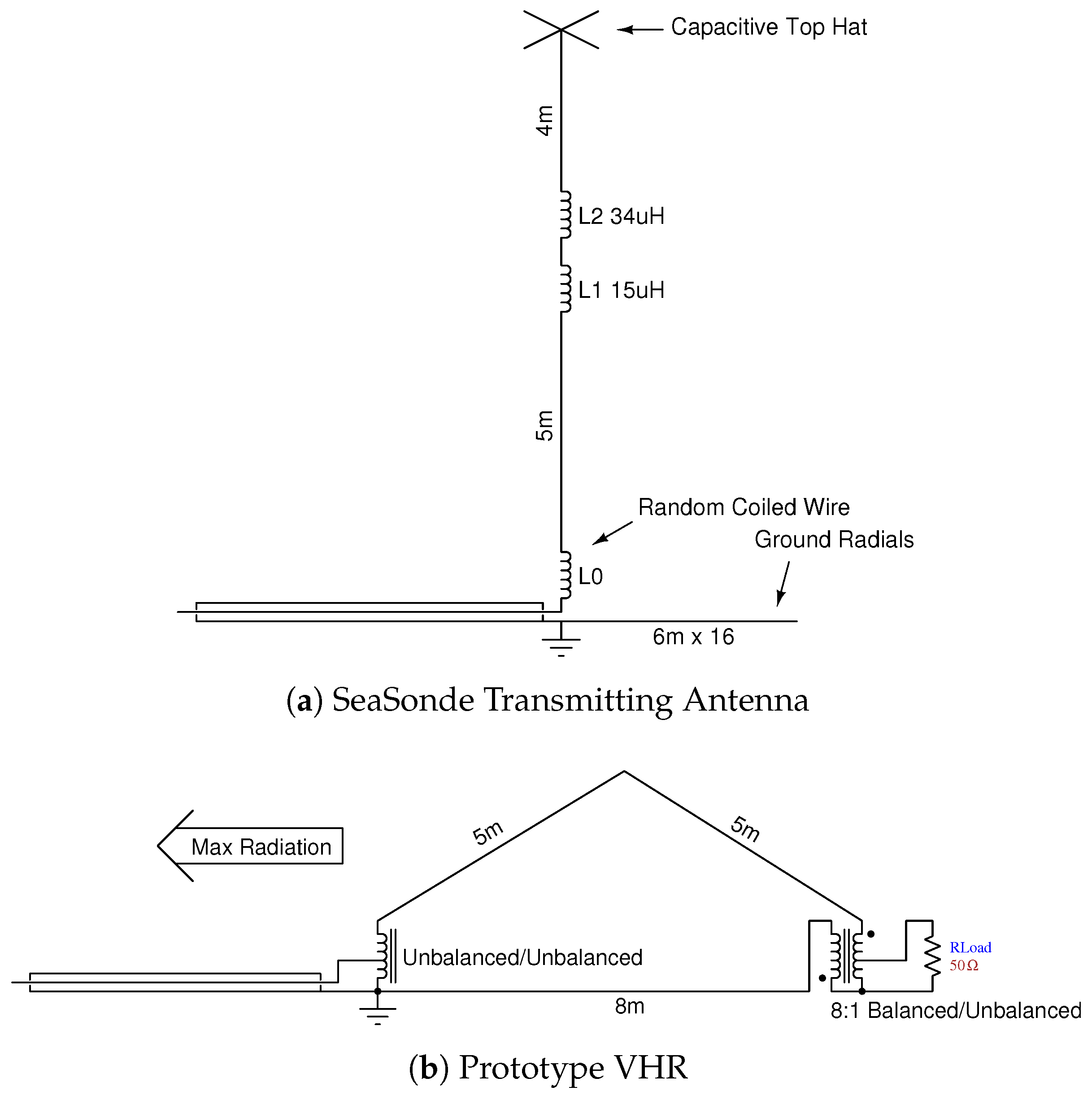
In its simplest design, the proposed directional transmit antenna, called Travelling Wave Loop Antenna or TWLA, requires a wave-guide, a load (or termination) resistance, a broadband feed-point impedance matching circuit, and a support structure (Figure 1).

It is based on the concepts of electrically small wire loop antenna and travelling wave propagation on a guiding structure [47,48,52,53,54,55,56].

The proposed directional transmit antenna is a triangular loop with a feed-point and resistive termination located at the two lower apices. For convenience, when adapting an existing SeaSonde system, it is possible to utilise the commercial SeaSonde transmit (TX) whip element with the centre loading coil removed, as both a support and one side of the triangular loop. The addition of two $1.6\mathrm{mm}$ 316 stainless steel wires, connected to the top and bottom of the whip, which meet at the third apex of the triangle where they are connected via a terminating resistive load, complete the antenna. In this geometry, the main radiating lobe is directed away from the termination load resistance back over the antenna feed-point (Figure 1c,d). Additional guy ropes are attached to the top apex in order to support the wire which is clamped to the top of the whip with a standard SeaSonde top-hat adaptor. Stainless steel hose clamps may also be used to make the required connection if the top hat adapter is not available. The TX whip acts both as a support structure and as part of the radiating element, in combination with the stainless steel wires.

2.3. Modelling and Simulation

Several antenna configurations were modelled and a number of prototypes tested before settling on the final design. Modelling the standard SeaSonde transmitter element was performed with the purpose of having a known reference to quantify the TWLA gain or loss. Although rather course, given the simplifications involved with modelling the environment and large number of unknown factors affecting measurements, the reference such as it is remains useful.

The geometries of candidate and reference antennas were modelled using xnec2c, a GUI version of the NEC-2 (Numerical Electromagnetics Code version 2.0 [58,59,60,61]) ported to the C programming language [62,63]. The cocoaNEC2.0 version 0.9.4.1 [64] was also used. NEC models antennas as combinations of individual straight wire segments automatically derived from a larger geometric description of the desired structures in a Cartesian coordinate system.

Our initial work and feasibility involved looking at simulation results of an electrically small Vertical Half Rhombic (VHR) design, on the basis of fundamental knowledge of travelling wave principals as applied to a full-scale sized Rhombic Antenna.

The VHR configuration (Figure 1b) is simple to implement with only three essential wires, but additional short elements were added for feed-point and terminating load for the convenience of trying other configurations without having to adjust the feed-point and load segment locations. Segment numbers and lengths were adjusted to keep them short with respect to the wavelengths of interest.

Software simulations for the vertical Half Rhombic were performed initially feeding the antenna at a single feed-point with unit voltage; the terminating load resistance was initially set to around $500\Omega$ and was adjusted while observing the affects on antenna radiation pattern, gain, feed-point impedance and frequency response over the $4\mathrm{MHz}$ and $5\mathrm{MHz}$ ITU bands, in particular, and wider frequency ranges, in general. These initial simulations were used to establish a starting point for prototype design and the associated field trials, and suggested that in general electrically small antennas typically have high losses in the order of ($-10\mathrm{dBi}$ to $-30\mathrm{dBi}$).

The conventional SeaSonde transmit antenna was modelled as simple 10 m long vertical wire fed at the antenna base; in these initial simulations, the centre load was not included. Later models include the centre loading coils. The unknown inductance $L_0$ at the base of the antenna, added in consideration of the random coiling of excess wire usually present, has not been modelled at this time.

Simulations were performed both for the standard SeaSonde transmitter element and the proposed TWLA with different configurations and environmental conditions, such as the simple linear cliff model, so as to develop an insight into the types of effects deployment site conditions may potentially produce.

2.4. Impedance Matching

Due to the termination and consequential lack of reflected energy at the feed-point of the antenna, the feed-point impedance is found to vary only a few Ohms over the entire radio determination band of interest. Small variations in feed-point matching such as those observed represent less than $1\%$ and therefore can be well matched with a broadband matching transformer. Initial modelling suggested the antenna should have a feed-point impedance of 400–500 $\Omega$ giving an impedance ratio of around 8:1 to 10:1. This translates to a turns ratio of $\sqrt{8}$:1–$\sqrt{10}$:1 $\approx$ 14:5–16:5.

Commonly available balun (balanced-unbalanced) designs employ a 1:2 turns ratio giving a 1:4 impedance ratio, deemed not particularly suited to this task.

Another common design of unbalanced-unbalanced transformer for high impedance loads employ a 1:7 turns ratio, with a two turn primary; however, this results in impedance matching steps of over $150\Omega$ per turn. A closer match to the desired 1:10 impedance ratio starting point can be obtained with a 5:16 turns ratio, resulting in a significantly smaller step size of a little over $50\Omega$ when adjusting the number of secondary turns.

Increasing the number of primary turns too greatly has a rapidly diminishing return as the inductance of the winding starts to rapidly increase. The potential for core saturation also may represent a problem since an increased number of turns represents a higher magnetic field for any given current and hence reduces the output power at which saturation will occur. Core saturation is a limiting feature of a balanced-unbalanced transformer design as operating above this point will produce heating and non-linear effects potentially producing unwanted harmonics.

Extrapolating from a typical 1:4 design by extending the secondary region of the windings around the toroid produces a balanced-unbalanced transformer at any desired integer turns ratio.

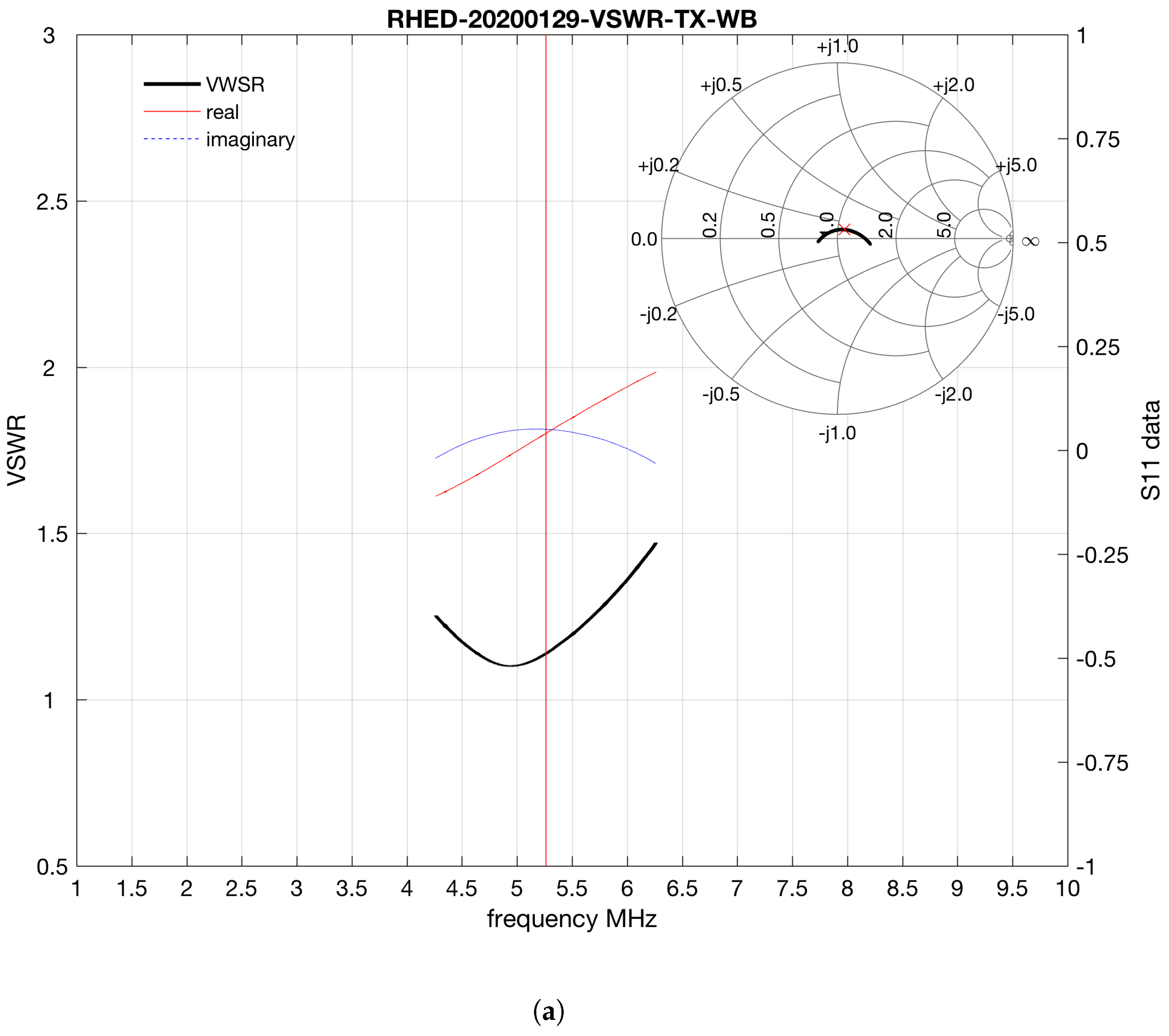
In the final installations, broadband matching of the antenna to the transmission line has then been carried out by adjusting the number of secondary turns on a custom high impedance matching unbalanced-unbalanced transformer for best Voltage Standing Wave Ratio (VSWR).

2.5. Geodetic and Plane Surveying

In combining information with Cartesian and polar model coordinates, local plane surveying data and GPS position data for signal level locations and flight path way points, it is necessary to be able to convert between Geodetic coordinates and an local Cartesian coordinate system. A most convenient local coordinate system is an East, North, Up (ENU) coordinate system centred on the antenna base where: $x\mapsto \mathrm{EAST}$, $y\mapsto \mathrm{NORTH}$ and $z\mapsto \mathrm{UP}$. This can be readily transformed into azimuth bearings for polar plots spherical coordinates three dimensional spherical plots. Model data and flight paths can be easily rotated to the correct orientation to correspond with the simulated model data and physical orientation of the antenna. Geodetic to Local and Local to Geodetic transformation routines were developed based on [65]. Local coordinate transforms are performed with basic linear algebra.

2.6. Antenna Pattern Measurements

We used the compact, battery-powered, programmable signal source as described in [66] attached to a commercially available programmable quad-rotor drone, to perform calibrations of the antenna beam patterns, and verify the correspondence between the modelled and measured antenna directionality and beam width. A similar approach is commonly used at HF and Ultra High Frequency (UHF) when antennas need to be tested and when large radiating structures are involved [67]. The only detraction of this approach is that it is difficult to separate the influences of the surrounding environment from those of the antenna design.

Initial calibration trials used a centre-fed dipole antenna which had two elements, each $2.1\mathrm{m}$ long, constructed from 18 gauge wire. This was later replaced by a similar length dipole antenna made by splitting the shield of a pre-terminated length of RG174 coaxial cable. The signal source was then attached at the bottom of the antenna so to keep the entire length of the antenna and not just one arm under tension. The signal source produces a $10\mathrm{mW}$ signals over a range of user-selectable frequencies in the HF band.

The drone was configured to fly at different elevations and fixed distance relative to the transmit antenna. In early flight plan way points were generated semi manually using the standard flight software supplied with the drone. Vertical profiles were also collected at selected bearing angles in an attempt to determine and quantify a possible enhancement effect of the cliffs and determine the vertical angle of maximum radiation. To gain more precise control, way point assignment has been undertaken using ENU coordinates and translated to geodetic coordinates. This is particularly of use when it is desired to fly vertical paths at specific azimuth angles either side of the antenna boresight.

Signal strength data as measured by the directional antenna were collected using a FieldFox hand-held RF vector network analyser operated in spectrum analyser mode. Three methods have been used to collect time synchronised signal level data:

• Complete spectra were recorded via the Field Fox LAN interface.
• Internal Recording of Real Time Spectra data with a FieldFox operating in Real Time Spectrum Analyser (RTSA) mode. Synchronisation was maintained with the Field Fox’s internal GPS clock.
• Reading the Field Fox marker values at the signal frequency and at an offset frequency to estimate the noise floor. Time is logged immediately before and after the scan and then the marker values are read.

When meteorological conditions were prohibitive (due for instance to strong wind conditions) and there was enough clear space around the antenna, walking patterns were performed with an hand-held GPS to record positions of the signal source around the antenna. Alternatively, the TWLA front-to-back ratio was quantified by collecting single scans at the expected antenna’s front and back lobe’s positions.

Signal data are assigned an interpolated ENU position corresponding to the time of the recorded spectrum data in order to derive the antenna beam pattern in a post-processing mode. ENU coordinated signal data positions are then translated into the Near and Far-Field modelling coordinate frames in order to obtain predicted signal levels for each location attributed to a measured signal level and provide the comparison between modelled and measured data.

Time synchronisation is critical as it is the only link between the signal data and the logged GPS flight data giving its position. Synchronisation is best achieved via GPS clock or Network Time Protocol (NTP). Timing errors may lead to an offset between the real position of the recorded signal and its attributed position. For this reason, and in analogy with the conventional approach used for the antenna pattern measurement in a SeaSonde HFR system, wherever possible the flight path was flown both clockwise and anticlockwise. This allows identification and estimation of synchronisation and potentially other errors caused by lagging of logged data or velocity dependent offsets and any other similar variations.

For the SeaSonde systems deployed in NSW, the signal source was set as closely as possible to the band centre frequency of $5.2625\mathrm{MHz}$ (typically $5.263\mathrm{MHz}$). For initial field and site testing carried out in Western Australia the source frequency was set to $4.463\mathrm{MHz}$, the centre of the ITU $4\mathrm{MHz}$ band currently used by these systems (Table 1). Reference noise floor data was collected at a frequency offset from the peak but within the ITU designated band. Signal to noise ratios are largely irrelevant to the actual drone pattern determination. However, they are most useful as an indications of when signal data may be invalid due to high noise levels, caused for instance by broadband or impulse interference noise during calibrations.

2.7. Field Test and Site Trials

For initial testing, a standard long-range SeaSonde antenna, including the stainless steel ground radials, was set up at the University of Western Australia’s field station in Shenton Park.

A prototype of the electrically small VHR design was also built for testing following the preliminary modelling. This design was supported from a guy wire of the standard SeaSonde antenna, the idea being to be able to easily alternate between the two for test and reference measurements.

The two antenna elements in the VHR prototype were made with $4\mathrm{mm}{}^2$ PVC insulated copper wire. The upper wire element was supported at its mid point from one of the SeaSonde antenna guy wires to form the apex of the prototype antenna. The remaining wire element was then stretched below to form the base of the triangular loop. A custom 8:1 balanced-unbalanced transformer feeding a commercial $1\mathrm{kW}$ $50\Omega$ test load was used for termination of the resulting wire loop. As well as being convenient this allows access for measurement of the power reaching and hence being dissipated in the test load. A portable MFJ tuner [68] was then used to match the antenna to a feed line at the $4.463\mathrm{MHz}$ test frequency. The antenna was connected to a FieldFox operated in spectrum analyser mode, and spectrum traces were streamed to a personal PC through the available Ethernet port while the programmable signal source [66] was used as reference signal to measure signal strength at the antenna’s front-back locations. A potentiometer was used to obtain the value for the termination resistor that optimised directionality and minimised the signal strength at the antenna’s desired back location.

The VHR was subsequently tested at Lancelin using the same set up, however with unsuccessful results. Following this initial site trial a more detailed “critical” view was taken of the VHR model results, which led to a significant modification of the antenna design.

A new site trial was performed at Lancelin in December 2018 when the TWLA prototype antenna was connected to the SeaSonde transmitter (Figure 2). Rather than modify the SeaSonde antenna for this one off test we included an extra vertical wire, since modelling suggested a negligible effect from the SeaSonde vertical element with the loading coil on the TWLA prototype. Two PVC coated copper wires were therefore supported from the top of the existing SeaSonde antenna both electrically connected to the top hat. One wire was extended down the outside of the mast to about $1\mathrm{m}$ from ground. The second wire was drawn to the rear of the antenna and secured with a rope to a peg. A base wire was stretched from the base of the SeaSonde mast also to the rear of the antenna. The two free wire ends were fitted into a connector to allow easy changeover between a high power termination load for transmission tests and a potentiometer for receive tuning tests.

Termination was by way of a 1:8 balanced-unbalanced transformer feeding a 50 Ohm unbalanced commercial test load (Figure 2c). A similar connector was used at the feedpoint (Figure 2b) to allow connection of the feedpoint matching unbalanced-unbalanced transformer. Feed-point matching was achieved by adding turns to the transformer while VSWR reduced and minimum VSWR was reached. Once adding a further turn caused VSWR to increase, the additional turn was removed and the tuning deemed complete.

In this test, bandwidth was set to $26\mathrm{kHz}$ consistently with the routine operational settings at the site, while software attenuation was gradually adjusted from 15 dB to 3 dB until Bragg signal could be detected in the data. This strategy was adopted in order to protect the transmitter final output amplifier from excessive reflected power in event of an unexpected fault resulting in antenna mismatch. The directive antenna was left in operations for a few hours, during which integration time was set to 15 min and left unchanged. This was necessary so to ensure reproducibility and consistency of Doppler resolution with data subsequently collected using the standard omnidirectional SeaSonde transmitter antenna configuration.

2.8. Site Deployments

Red Head Point is located in a natural reserve area approximately 100 km to the North of Sydney. The receive and transmit antennas are installed in a relatively flat, small and partial clearing close to the cliff edge. The presence of sensitive vegetation is a major operational constraint at this particular site.

A number of modifications to the TWLA were carried out for improved durability, leading to the final form of our design detailed in Section 2.2. Prior to installation of the new TWLA we attempted to record the pattern of the unmodified antenna as well as collect reference signal data. The signal source was set to the $5\mathrm{MHz}$ mid-band frequency $f_c$ (Table 1).

During the follow up visit to site the loading-coil was reinstalled and the SeaSonde transmitter pattern re-measured and reference level data collected. The directional antenna was then reinstalled and the direction adjusted by ${20}^{\circ }$ in order to bring it as close as possible to perpendicular to the baseline between the systems. Adjustment by the full ${30}^{\circ }$ was not possible due to the unfortunate position of the surrounding vegetation.

The design was modified to suit the site topography at SEAL which is located on a small flat area at the base of a steep slope overlooking a cliff. This high degree of slope in the direction of the loop necessitated raising the termination which altered the final loop shape.

Where possible the opportunity to repeat and improve APM has been undertaken during subsequent sites visits. Attempts to repeat measurements at SEAL, however, have been frustrated by weather, equipment malfunction and a short drone flight operational window which does not allow for correction of any but the most minor of difficulties. VSWR data were collected at our most recent visit.

3. Results

3.1. Antenna Modelling

An overview of free-space far-field simulated patterns for the SeaSonde Transmitting antenna, VHR and final TWLA antennas deployed at RHED and SEAL are presented in Figure 3, Figure 4, Figure 5 and Figure 6. These figures show the plan and elevation views of the patterns along with perspective views of the overall, horizontal and vertical polarization components of the radiation field. The maximum calculated directional gain for each of the final models are summarised in (

Table 2. Comparison of numerical simulation results for the simplified SeaSonde antenna and alternate layouts for the directive antenna. Monopole refers to the SeaSonde transmitter; Prototype refers to the preliminary test, and Prototype ×2, Prototype ×4 refer to the prototype scaled twice or four-times. RHED and SEAL refer to the approximate layouts as currently deployed at those field sites. See (Figure 1).

Design	Perieter	Loop Area	Max Gain	Notes
	(m)	(m2)	(dBi)
Monopole (Approx.)	N/A	N/A	1.08
Prototype	18.2	16.0	−21.15
Prototype ×2	36.4	64.0	−11.02
Prototype ×4	72.8	256.0	0.21	Loss of Directivity
RHED	24.2	26.1	−18.04
SEAL	24.2	26.1	−14.33

) along with some statistics of each design, such as the perimeter and the loop areas. It is worth noting that an over-scaled design such as the Prototype ×4 caused a loss of directivity in the simulated pattern.

One of the first notable results from early modelling was the direction of maximum radiation being away from the termination resistor. This was notable since full size Rhombic and other travelling wave antennas are known to receive signals more strongly from the direction of the terminating load towards feed-point and emit signals oppositely [48,51]. Evidence so far suggests that while the loop size is small the preferred radiation direction is away from the terminating resistor and that this transitions to the opposite as dimension are increased to the order of $\lambda {}_{f_c}^{}$.

Results of the numerical simulations suggest that in general the TWLA antenna has a desirable broad beam directional pattern with predominantly vertical polarization directed towards the sea surface. Simulations also suggest that the TWLA does presents a small horizontally polarized component (Figure 4e, Figure 5e and Figure 6e). In our final designs, however, this is mostly directed downwards and to the sides, where it undergoes rapid attenuation and reduced low angle propagation resulting from the cancellation of the horizontal components of the electric field upon reflection from horizontal surfaces. As expected there is no discernible horizontal component present in the simulation results for the SeaSonde transmit antenna which has no horizontal radiating structures (Figure 3e).

3.2. Field Test and Site Trials

FieldFox data (not presented here) collected during the preliminary Field test at Shenton Park showed front-to-back suppression (20 dB) as expected from preliminary simulations for the VHR design.

Subsequently the preliminary site trial of the VHR prototype conducted at Lancelin failed to produce Bragg signal regardless of the transmit power that was fed to the antenna.

Following design modifications the Lancelin trial of the TWLA as detailed in Section 2.7 proved successful. Examples of Bragg spectra collected through receive channel 3 (the so called “monopole” in standard SeaSonde operational jargon) with the conventional and the prototype directive antenna are provided in (Figure 7).

An attenuation setting of $3\mathrm{dB}$ produced a $22\mathrm{W}$ RF (radio frequency) signal and an operational range of approximately $200\mathrm{km}$. A similar range was achieved with the existing $4\mathrm{MHz}$ SeasSonde transmitting antenna when fed with $10\mathrm{W}$ RF signal at an attenuation setting of $8\mathrm{dB}$. Both signal measurements were performed at output of the Power Amplifier (PA). Closer inspection of the data presented in (Figure 7) reveals a $5.6\mathrm{dB}$ difference in the mean peak signal levels within the Bragg regions of the first 60 range cells. In addition to the $3.5\mathrm{dB}$ difference in measured transmitter output power this represents an approximate $9\mathrm{dB}$ difference between the antennas. Compared with the $-15\mathrm{dB}$ difference expected from simulation (Table 2), this represents a discrepancy of $6\mathrm{dB}$ (about 4:1), which, although quite large, most likely remains within very broad modelling and measurement uncertainties, which are difficult to quantify.

There is a minor variation in backscatter strength in the second-order region between the directive and the omnidirectional antenna (Figure 7b), which is most likely originating from the increased radiation efficiency in the conventional transmitter in combination with an increased sea-state associated with the local sea-breeze wind regime [42].

Two spectra scans collected with the FieldFox at locations to the front and rear of the antenna confirmed a $21\mathrm{dB}$ front-to-back ratio (Figure 8) as for the initial trials, also consistent with simulation.

3.3. Final Deployments

Two alternate arrangements were implemented for the field deployments at the New South Wales SeaSonde sites due to the different characteristics of the each location.

At Red Head the antenna is shaped more closely to a right-angled triangle with 10 m “hypotenuse”, and 6 m (9 m) “catheti”, resulting in an overall loop perimeter of approximately $25\mathrm{m}$. (Figure 1c). Fine tuning aimed at optimizing the front-to-back ratio was achieved with a measured resistance of $1.1\mathrm{k}\Omega$ termination load. A $1.125\mathrm{k}\Omega$ load was then fabricated using a set of 16, $18\mathrm{k}\Omega$, 1 W carbon resistors in parallel arrangement. Subsequently a 64 resistor version was fabricated by series connection of two parallel sets of 16 resistors to allow for higher power testing but this has not really been required. A more convenient arrangement of 32, $18\mathrm{k}\Omega$ resistors would likely represent a better balance between ease of fabrication and a slightly higher power rating when testing up to $15\mathrm{W}$ RF power continuously and allow short duration of higher power tests.

Voltage standing wave ratio (VSWR) data along with real imaginary parts of the complex reflection scattering coefficient ($s_{11}$) for this antenna are given in (Figure 9a) for a $2\mathrm{MHz}$ band around the centre frequency ($5.2625\mathrm{MHz}$) of the $5\mathrm{MHz}$ ITU band. Optimal frequency tuning is achieved at $4.4936\mathrm{MHz}$ ($\mathrm{VSWR}=1.09$), slightly offset in frequency to the desired operating frequency ($5.265\mathrm{MHz}$) where $\mathrm{VSWR}=1.13$. Phase response within the band is flat.

The TWLA antenna deployed at Seal Rocks has the shape of a triangle with $8\mathrm{m}$ long catheti and the $9\mathrm{m}$ standard SeaSonde antenna to complete the loop, for a total length of $25\mathrm{m}$ (Figure 1d). Optimal tuning for the termination loading was more difficult to obtain in comparison with the deployment at the RHED site, mostly for the complexities of the installation location. There was little in the way of a discernible dip in signal so it was adjudged to use the same $1.125\mathrm{k}\Omega$ $\approx 16\mathrm{W}$ load as was initially installed at RHED. VSWR data for this antenna, shown in (Figure 9b), returns $\mathrm{VSWR}=1.52$ at the work frequency, with a well defined minimum ($\mathrm{VSWR}=1.06$) at $6\mathrm{MHz}$.

3.4. Measured Antenna Patterns

We have performed repeated drone based pattern measurements of our installed antennas where time and weather conditions have permitted, including the conventional SeaSonde transmit antenna (Figure 10). A summary of numerical results generated from data collected over a number of site visits since installation is given in (

Table 3. Drone pattern measurement results summary for pattern measurements performed at RHED and SEAL HFR stations. TWLA identifies the directional antenna. The initial installation at RHED was directed 60° from the baseline towards SEAL which is the centre of the optimal sea coverage area of the two sites. It was subsequently decided that for future coverage to the south and to reduce the signal directed overland to the north that the directionality should be directed 90° to the baseline.

Site	Antenna	Date	Normalization	$\mathit{\mu }$Noise	Front-to-Back		Range	Elevation
			Factor		Ratio (dB)
		(YYYYMMDD)	(dBm)	(dBm)	Simulation	Data	(m)	(m)
RHED	TWLA	20190530	−111.89	−125.99	10	>10	100	50
RHED	Mono	20190531	−74.72	−107.55	10	>10	100	50
RHED	TWLA	20191022	−81.09	−111.62	10	>25	150	50
RHED	TWLA	20191023	−80.93	−107.53	10	>25	150	50
RHED	TWLA	20200129	−82.81	−127.91	10	30	150	50/70
SEAL	TWLA	20191025	−81.27	−111.69	18	N/A	250	50

).

(Figure 11a) for instance shows results of the near field pattern measurement performed on 22 October 2019 at Red Head site after further refinement to the design. The plot shows the level of the signal source (blue markers) and the noise floor levels (red markers), normalized to the maximum received received amplitude ($-81.09\mathrm{dBm}$), along with model calculated electric field squared at same elevation and range as the drone (green markers), also normalised by their maximum amplitudes. Signal strength values and background noise levels are overlain to coastline orientation, with blue (green) arrow indicating the expected direction of the main lobe towards the ocean (the paired SeaSonde site at the Seal Rocks lighthouse). It should be noted that the blue arrow in (Figure 10) is shown in the direction of the initial TWLA installation at that site and is coincidentally pointing perpendicular to the cliff and thus in the direction of maximum gain given the influence of environmental factors. The antenna of course is expected to be omnidirectional. The grey lines in this and similar plots correspond to significant coastal features digitised from aerial photography and scaled such that the $0\mathrm{dB}$ circle corresponds to the drone flight path. Dark green points are model predicted near field data corresponding to the flight path while Magenta points are linear cliff model far field data for the corresponding flight path azimuth and elevation.

The correspondence between simulated model fields and observed signal levels over the ocean is significant. In this sector, differences in measured signal levels between the two drone passes are not significant and likely to be the result of differential tilting of the signal source antenna due to the relative wind direction and drone velocity. Calibration data suggest that a 3 dB antenna beam width in the horizontal plane for this specific elevation angle is approximately ${120}^{\circ }$.

Over land, the signal strength drops off quickly reaching or falling below the noise floor level (approximately $-30\mathrm{dB}$). This is particularly true at low elevations where the signal path is affected by the proximity of vegetation. Here, the front-to-back ratio from field data (at least <−25 dB) is even more pronounced than the expected simulation value of around $-10\mathrm{dB}$.

Calibration results remain consistent over time. A second APM performed at the RHED a few weeks after installation revealed the overall shape was unaltered, with the most significant difference between the two runs being a different (i.e., higher) noise floor level between the measurement runs. This could be due to a higher noise floor or a weaker test signal reception. Consistent with the previous measurements, the $3\mathrm{dB}$ beam width over the ocean was approximately ${120}^{\circ }$, the signal level over land dropped to the noise floor threshold, or below, and the front-to-back ratio was also consistent. This hypothesis is supported by the results of the pattern measurement of the standard SeaSonde transmit antenna (Figure 10), that was performed at Red Head in May 2019 with the purpose of further assessing the modelling capabilities and possibly quantify the loss or gain of the proposed TWLA against the conventional transmit approach.

Both patterns show some attenuation over land. This can be seen to increase as the proportion of overland to over water path changes as the drone path approaches and crosses the coast. In this case the signal appears to be $10\mathrm{dB}$ lower than expected from modelling and is clearly evident to the rear of the antenna, which is attributed to the increased signal loss over land. In addition the land to the rear of the antenna is sloped upwards which may account for the greater than expected attenuation to the rear.

Flying the drone at different altitudes relative to the transmit antenna suggested that the cardioid pattern can be observed at lower elevation angles. This is illustrated for instance in (Figure 11b) which merges the transmit pattern calibration for two elevations ($50\mathrm{m}$ and $70\mathrm{m}$ relative to the antenna base).

An example of Doppler spectrum, collected using the directional transmit antenna as transmitter, receive channel 3 as receiver, and representative of a 30 min integration cycle, is presented in (Figure 12), along with the corresponding radial velocity map. Integration time was set to 1024 s, bandwidth was $11.028\mathrm{kHz}$, corresponding to a radial range resolution of $13.591\mathrm{km}$, sampling rate was 1 Hz, output transmit power at the amplifier was <4 $\mathrm{W}$.

Measuring the complete directional antenna pattern at the Seal Rocks location was not possible due to site characteristics, the lack of flying permits over the National Park area, and the limited flight-time window due to the presence of a restricted airspace in the vicinity of the lighthouse limiting operational hours to those between sunrise and 0900 local time. Attempts to repeat measurements were also unsuccessful due to failures to the signal source power supply, losses of telemetry, or adverse meteorological conditions. However, even with all limitations, the partial data still provided a relatively good match between the field measurement data and the model simulations.

Results of the preliminary drone antenna near field pattern measurement are provided in (Figure 13), while an example of the data coverage with the directional antenna (Doppler spectrum and corresponding radial velocity map) is provided in (Figure 14). Consistently with the simulations, at this elevation angle the cardioid pattern is not well defined although an approximate $-20\mathrm{dB}$ drop is expected for the front-to-back ratio (Figure 13). The measured data show agreement with the expected pattern between ${180}^{\circ }$–${250}^{\circ }$ and ${45}^{\circ }$–${90}^{\circ }$; however, the match is poorer at other bearings. This mismatch may be associated with the effects of the island offshore and in the direction of the antenna’s main lobe.

4. Discussion

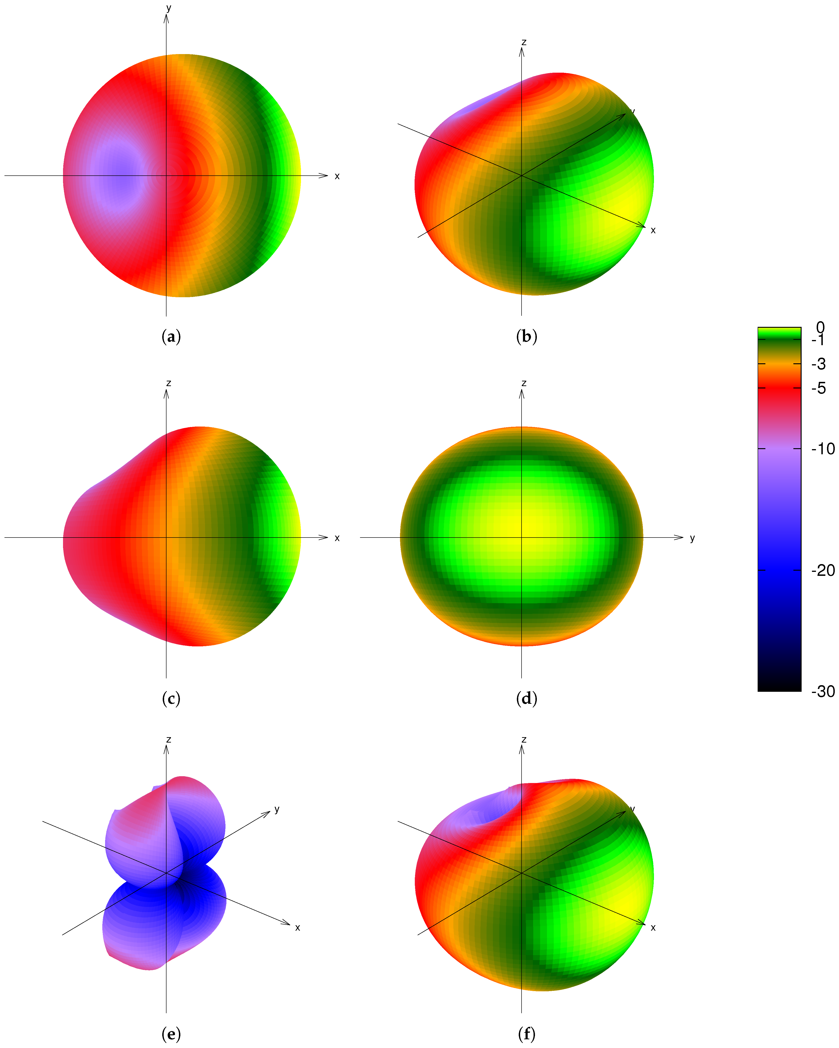
Simulations with the NEC-2 [58,59,60,61] software demonstrate that the TWLA design combines the desired characteristics of broad beam directivity, with predominantly vertical polarization and the required level of compactness. There are strong similarities between patterns shown in Figure 4, Figure 5 and Figure 6, indicating an independence of the precise antenna geometry. This suggests some flexibility in the final design and that the antenna may be easily adapted to varying environmental constraints without significantly altering its characteristics directionality.

The final model results for the VHR prototype are interesting as they show an upward direction of the main lobe which would have resulted in a further reduction of the radiation reaching the ocean surface beyond the already steep $-21.15\mathrm{dBi}$ maximum gain. This may be an even more compelling reason for the failure of the VHR prototype to produce Bragg scattering results.

The upward direction of signal was not noticed in our initial simulations. It was masked by the use of various ground plane modelling options. These options at first appear useful but in actual fact are more applicable to sky-wave propagation thus they disguise the true direction of radiation as it leaves the antenna structure. This has the affect of rendering the radiation patterns from the VHR and two final design TWLA antennas inaccurately similar.

An additional inaccuracy is that of the flat ground plane model not representing correctly the curvature of the earth. The downward angle to the horizon is small; however, it is this downward radiation which is responsible for developing the ground wave propagation on which HFR is reliant. Any radiation above the horizontal is at its closest to the earth at the antenna base and will not interact with the surface unless reflected back to earth by the ionosphere. Ionospheric reflections are generally beyond operational range for HFR; however, in long-range systems this is not the case and such reflection often cause significant interference limiting the usable range while present.

The final design of the TWLA is composed of a triangular loop in which the SeaSonde transmit element is both part of the radiating loop and the supporting structure. The shape is easily implemented on site using the guy ropes and the existing SeaSonde mast as support structures and as part of the radiation loop, provided that the coil between the two fibreglass sections is removed to avoid undesired loading of the vertical section of the resulting loop. We acknowledge that there is considerable scope for optimisation of the triangular shape presented here and that more tests and simulations may lead to further innovation and improvement especially if considering the design afresh. In the present, however, we are satisfied with a convenient working solution resulting from a quick and straightforward modification to existing infrastructure.

Of the possible parameters controlling antenna performance for a given geometry, two were determined to be suitable for adjustment on site: the termination resistance required to maximise the front- to-back ratio, and the antenna matching to the transmission line. These parameters are largely dependent on antenna geometry and ground conditions. A simplified modelling approach may not be suited to predict their optimum values given the nature of these aspects of the installations. So far, good results have been obtained by initially installing a carbon film potentiometer (wire wound potentiometers are unsuitable due to their inductive characteristics) as the terminating resistor and adjusting it for minimum pick up of a signal source placed to the rear of the antenna. Once this value has been determined a suitable higher power, terminating load can be installed in its place.

The desired directionality and wide-beam pattern towards the ocean are consistently reproduced between the simulations and the field measurements performed with an autonomous drone and a known signal source. Repeated measurements also show that the directional pattern is in general stable and is not particularly affected by changes in environment (i.e., ground) once installed and finalised.

Efficiency is computed by the software packages as a ratio of the input power to the radiated power through the antenna, and is in general low. This is clearly seen in the simulation statistics reported in Table 2. Compared to the conventional SeaSonde transmit antennas, modelling suggests a loss of approximately 15–$19\mathrm{dB}$ for the TWLA, and an overall antenna efficiency of around $23\%$. While there is no direct correlation between the physical dimensions of an antenna and the effective aperture and hence its efficiency, it is worth noting that increasing (doubling) the size of the prototype increased the gain by about $10\mathrm{dB}$ (a factor of 10). Such increases cannot be continued indefinitely as continuing to increase the size progressively degrades directivity as the antenna gradually transitions to the classic travelling wave/terminated long wire mode. The exact transition point has not been determined, and is likely to vary depending on individual antenna geometry. However, the transition generally occurs as the length of the loop increases to the order of $\lambda {}_{f_c}^{}$. In the case of the VHR more of the energy becomes directed at the ground at scales above not much above 2:1 of our dimensions for the $5\mathrm{MHz}$ band. A larger antennas would pose increased engineering challenges in the fabrication and deployment stages. Our present design is constrained to fit with the existing installed antennas and requires minimal reconfiguration to create a working solution. The effect of increasing the size relative to wavelength can best be observed by scanning the excitation frequency over the HF spectrum while keeping the antenna dimensions constant.

We acknowledge that the TWLA is less efficient when compared to a phased-array arrangement or the conventional omnidirectional SeaSonde antenna; however, this loss is readily compensated for by the output power usually available at a HFR site, the ease of installation, reduced space requirements, and the suitable directional pattern. Rather than being a problem, the additional attenuation turns out in fact to be an advantage. Due to difficulties encountered collecting suitable data there is still a large uncertainty associated with confirming the relative gain and efficiency of the TWLA with that of the standard SeaSonde transmitting antenna. Simulation predicts something on the order of $10\mathrm{dB}$ to $15\mathrm{dB}$ depending on design while estimates from data collected at Lancelin indicate the difference is around $9\mathrm{dB}$. This is potentially within the uncertainty of our experiments to date. Difficult site conditions and limited testing windows have affected the quality and quantity of applicable data. Neither has it been possible to conveniently repeat before and after modification measurements to properly asses their uncertainty.

In the specific case of the NEWC installations where the systems operate at very low power, the minimum controllable output levels of the SeaSonde transmitter were already reached and no further reductions were possible via software controlled attenuation. Having attenuation in the antenna system saves adding attenuation in the feed line or modification of the transmitter power amplifier and sensing.

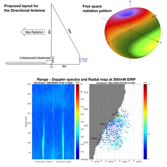
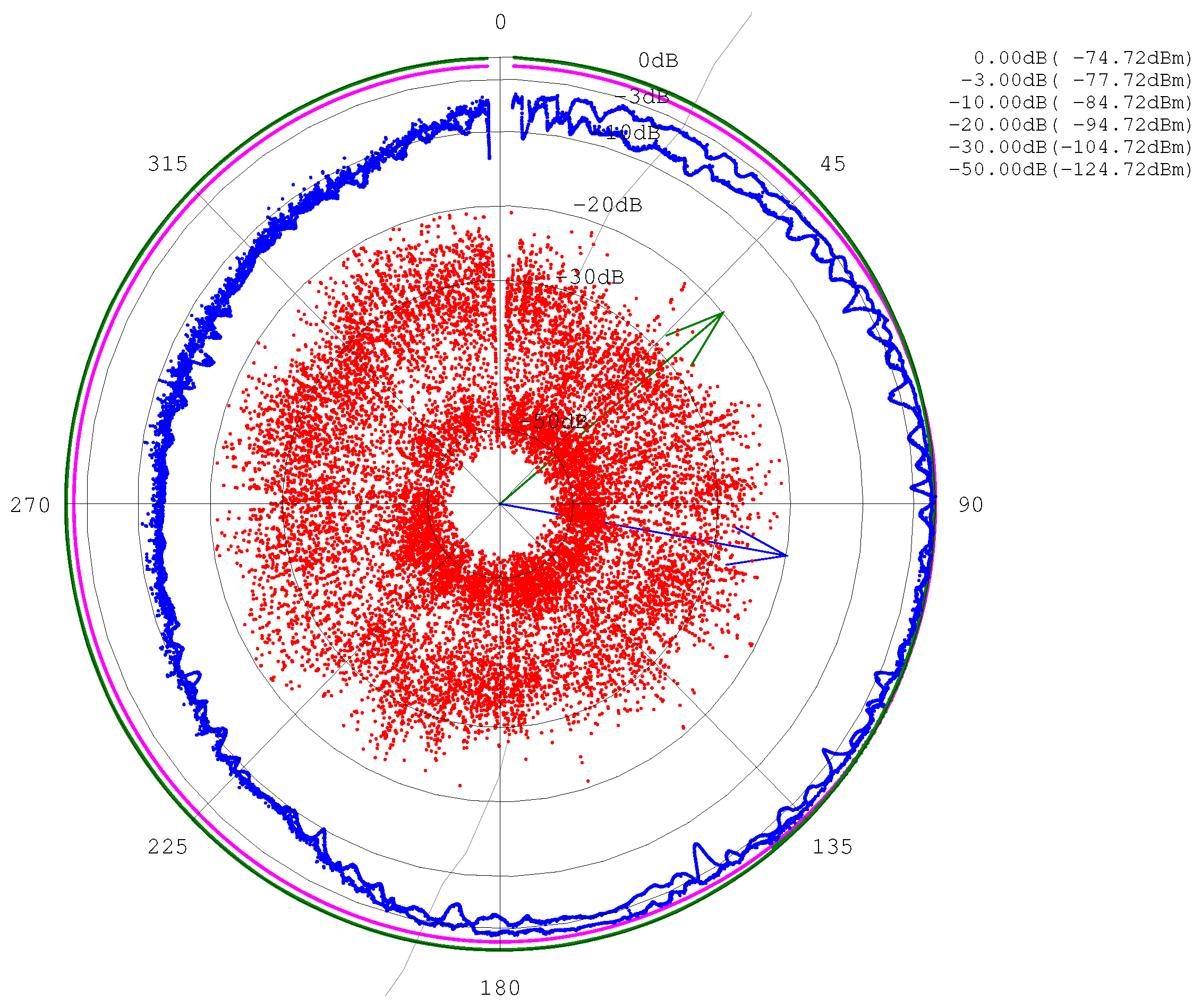
Qualitatively and quantitatively, there is little difference between the Doppler spectra collected during the Lancelin field trial (Figure 7), Bragg signal strength, noise floor levels, and signal-to-noise ratio statistics for the first-order Bragg regions. These can be easily derived from the diagnostics output in the SeaSonde proprietary software. The only notable difference is the perhaps slightly higher background noise associated with (Figure 7b) but this is not a direct result of the transmit antenna which is not a direct part of the received signal path or transmit antenna directionality. It is more likely to be natural variation in atmospheric or thermal background noise associated with the course of the day. Results from both the field trials of the prototype and the final deployment have demonstrated that operational ranges can still reach 200 km offshore at a fraction of the transmitted EIRP (<300 $\mathrm{mW}$, when considering transmission line loss in addition to the $10\mathrm{dB}$ to $15\mathrm{dB}$ gain loss compared to the standard transmit antenna) than that which is conventionally used. Example of data (Bragg peaks and radial velocity maps) collected with low to extremely-low power in (Figure 12 and Figure 14) support this, along with available the radial diagnostics data output of the conventional SeaSonde HFR software (not shown here).

Additional advantages of the low transmit power are the following:

• reduced interference within the ocean Bragg regions from ionospheric reflections;
• reduced interference to land-based services with HFR signal falling below the typical noise floor level at some monitored sites.

5. Conclusions

This paper documents the implementation of a compact directional antenna for HFR applications within the long-range (4 MHz and 5 MHz) ITU radiodetermination bands. We have presented the results of the field measurements and antenna model simulation to help validate and explain or our design. The results indicated that:

• Compact directional transmit antennas for High Frequency ocean RADARs can be implemented successfully, in fulfilment of the relevant international regulations. The proposed design has successfully incorporated the concepts of an electrically small wire loop antenna and travelling wave propagation on a guiding structure resulting in an easily deployed, relatively compact, in field modification to provide directional transmission.
• In the proposed design, the travelling wave loop antenna (TWLA) consists of stainless steel wires and a wired fibreglass mast as radiating elements; a terminating load; and a broadband matching transformer at the feed-point. It requires a support structure, which in the present design becomes a part of the antenna. We used a standard low-frequency SeaSonde transmit antenna mast (after removing the centre coil between the upper and lower sections) with the dual purpose of providing structural support to the TWLA, and as part of the antenna loop. In this way, the increased dimensions of the antenna loop improved the antenna radiating capacity, increased the coupling to the ocean and allowed for Bragg spectra to be collected.
• The antenna was designed using freely available open-source software. Antenna pattern simulations and sensitivity tests were performed in order to optimize the front-to-back ratio thus minimizing unwanted radiation over land. Antenna design and signal cancellation over land were further validated with field measurements, at both the prototype level and final deployment stages.
• The results of the field calibrations with a commercial drone and a programmable signal source confirmed the agreement with the NEC-2 software simulations. Repeated drone calibrations also confirmed that the directional patterns were stable over time. Antenna pattern measurement of the conventional SeaSonde transmit pattern were also performed at one of the SeaSonde sites, which showed a 10 dB loss over land due to vegetation and terrain.
• In comparison with conventional SeaSonde transmit antennas, the TWLA has low radiation efficiency, typically around 15 dB lower by comparing simulated maximum gain. However, these factors are not of concern since the lower radiation efficiency can be compensated by an increase in output power well within capability of a commercial SeaSonde system. This is especially true given our field deployments confirm that the effective coupling to the ocean still occur at low EIRP estimated to be below $300\mathrm{mW}$, with operational ranges up to 200 km.
• Operational settings of the Australian IMOS SeaSonde systems suggest that good range remain achievable at reduced transmit power levels. This gives the multiple benefits of reducing in-band interference to other services, further limiting unwanted emissions over land, and significantly reduce contamination from ionospheric reflections in the Doppler spectra with overall increase in data quality. A not insignificant detraction of the low-power operation mode is the limited energy in the second order Bragg spectral region, which limits the application of ocean wave inversion only to periods of well-developed sea conditions.
• This antenna design may be readily scaled for operation at other frequencies. Thus operation on any ocean HFR band should be possible unless limited by other factors.
• It remains untested if the TWLA may be successfully co-located with a SeaSonde receiving antenna. For SeaSonde systems operating in the upper portion of the HF spectrum (above $9\mathrm{MHz}$), co-location of the transmitting and receiving antennas permit a degree of compactness which will be lost if this co-location is not possible.
• There is potential for application in a WERA receiver array where the directive pattern may assist in reducing interference from strong terrestrial signals originating inland of the array.
• Indications are that the TWLA does not require a ground plane for operation.

References

1. Roarty, H.; Cook, T.; Hazard, L.; George, D.; Harlan, J.; Cosoli, S.; Wyatt, L.; Alvarez Fanjul, E.; Terrill, E.; Otero, M.; et al. The Global High Frequency Radar Network. Front. Mar. Sci. 2019, 6, 164. [Google Scholar] [CrossRef]
2. Huang, W.; Gill, E.W. HF Surface Wave Radar. In Wiley Encyclopedia of Electrical and Electronics Engineering; Webster, J.G., Ed.; John Wiley and Sons: Hoboken, NJ, USA, 2019; pp. 1–11. [Google Scholar] [CrossRef]
3. Fujii, S.; Heron, M.; Kim, K.; Lai, J.W.; Lee, S.; Wu, X.S.; Wu, X.; Wyatt, L.; Yang, W.C. An overview of developments and applications of oceanographic radar networks in Asia and Oceania countries. Ocean Sci. J. 2013, 48, 69–97. [Google Scholar] [CrossRef]
4. Barrick, D.E.; Evans, M.W.; Weber, B.L. Ocean Surface Currents Mapped by Radar. Science 1977, 198, 138–144. [Google Scholar] [CrossRef]
5. Hammond, T.M.; Pattiaratchi, C.B.; Eccles, D.; Osborne, M.J.; Nash, L.A.; Collins, M.B. Ocean surface current radar (OSCR) vector measurements on the inner continental shelf. Cont. Shelf Res. 1987, 7, 411–431. [Google Scholar] [CrossRef]
6. Paduan, J.D.; Washburn, L. High-frequency radar observations of ocean surface currents. Annu. Rev. Mar. Sci. 2013, 5, 115–136. [Google Scholar] [CrossRef] [PubMed] [Green Version]
7. Shearman, E. A review of methods of remote sensing of sea-surface conditions by HF radar and design considerations for narrow-beam systems. IEEE J. Ocean. Eng. 1986, 11, 150–157. [Google Scholar] [CrossRef]
8. Stewart, R.H.; Joy, J.W. HF radio measurements of surface currents. Deep. Sea Res. Oceanogr. Abstr. 1974, 21, 1039–1049. [Google Scholar] [CrossRef]
9. Li, Z.; Wen, B.; Tian, Y. Design and Implementation of a Dual-Frequency Compact Antenna System for HF Radar. IEEE Antennas Wirel. Propag. Lett. 2017, 16, 1887–1890. [Google Scholar] [CrossRef]
10. Tian, W.; Wen, B.; Tan, J.; Li, K.; Yan, Z.; Yang, J. A new fully-digital HF radar system for oceanographical remote sensing. IEICE Electron. Express 2013, 10, 14. [Google Scholar] [CrossRef] [Green Version]
11. Teague, C.; Vesecky, J.; Hallock, Z. A comparison of multifrequency HF radar and ADCP measurements of near-surface currents during COPE-3. IEEE J. Ocean. Eng 2001, 26, 399–405. [Google Scholar] [CrossRef]
12. Zhao, C.; Chen, Z.; He, C.; Xie, F.; Chen, X.; Mou, C. Validation of Sensing Ocean Surface Currents Using Multi-Frequency HF Radar Based on a Circular Receiving Array. Remote Sens. 2018, 10, 184. [Google Scholar] [CrossRef] [Green Version]
13. Lipa, B.; Nyden, D.B.; Ullman, E.; Terrill, E. SeaSonde radial velocities: Derivation and internal consistency. IEEE J. Ocean. Eng. 2006, 31, 850–861. [Google Scholar] [CrossRef]
14. Li, Z.; Tian, Y.; Wu, S.; Wen, B. Design of a Dual-Frequency Center-Fed Transmitting Antenna for Compact HF Surface Wave Radar. IEEE Antennas Wirel. Propag. Lett. 2018, 17, 1890–1894. [Google Scholar] [CrossRef]
15. Gurgel, K.W.; Antonischki, G.; Essen, H.H.; Schlick, T. Wellen Radar (WERA): A new ground-wave HF radar for ocean remote sensing. Coast. Eng. 1999, 37, 219–234. [Google Scholar] [CrossRef]
16. Flament, P.J.; Harris, D.; Flament, M.; Fernandez, I.Q.; Hlivak, R.; Flores-vidal, X.; Marié, L. A Compact High Frequency Doppler Radio Scatterometer for Coastal Oceanography. In Proceedings of the AGU Fall Meeting Abstracts 2016, San Francisco, CA, USA, 12–16 December 2016. [Google Scholar]
17. Kirincich, A.; Emery, B.; Washburn, L.; Flament, P. Improving Surface Current Resolution Using Direction Finding Algorithms for Multiantenna High-Frequency Radars. J. Atmos. Ocean. Technol. 2019, 36, 1997–2014. [Google Scholar] [CrossRef]
18. Wyatt, L.R.; Green, J.J.; Middleditch, A.; Moorhead, M.D.; Howarth, J.; Holt, M.; Keogh, S. Operational Wave, Current, and Wind Measurements With the Pisces HF Radar. IEEE J. Ocean. Eng. 2006, 31, 819–834. [Google Scholar] [CrossRef]
19. Wang, W.; Gill, E.W. Evaluation of Beamforming and Direction Finding for a Phased Array HF Ocean Current Radar. J. Atmos. Ocean. Technol. 2016, 33, 2599–2613. [Google Scholar] [CrossRef]
20. de Paolo, T.; Terrill, E. Skill Assessment of Resolving Ocean Surface Current Structure Using Compact-Antenna-Style HF Radar and the MUSIC Direction-Finding Algorithm. J. Atmos. Ocean. Technol. 2007, 24, 1277–1300. [Google Scholar] [CrossRef]
21. Heron, M.L.; Helzel, T.; Prytz, A.; Kniephoff, M.; Skirving, W.J. PortMap: A VHF ocean surface radar for high spatial resolution. In Proceedings of the Europe Oceans 2005, Brest, France, 20–23 June 2005; Volume 1, pp. 511–515. [Google Scholar] [CrossRef]
22. Huang, W.; Liu, X.; Gill, E.W. Ocean Wind and Wave Measurements Using X-Band Marine Radar: A Comprehensive Review. Remote Sens. 2017, 9, 1261. [Google Scholar] [CrossRef] [Green Version]
23. Codar Ocean Sensors. SSRS-100 Specification, v5, Rev 12/2016. Available online: http://www.codar.com/SeaSonde_Remote-Unit_specs_config_options.shtml (accessed on 1 October 2019).
24. Barrick, D.; Long, R. Twin Transmit Configuration; Codar Ocean Sensors: Mountain View, CA, USA, 2014. [Google Scholar]
25. Gupta, A.; Grant, D.S.; Fickenscher, T.; Karstadt, P. An efficient Electrically Small Antenna at HF band. In Proceedings of the Asia-Pacific Microwave Conference 2011, Melbourne, Australia, 5–8 December 2011; pp. 856–859. [Google Scholar]
26. Baker, J.; Iskander, M.F.; Yun, Z.; Evans, M.; Johnson, J.; Elsheakh, D. High performance compact antenna for HF radar. In Proceedings of the 2009 IEEE Antennas and Propagation Society International Symposium, Charleston, SC, USA, 1–5 June 2009; pp. 1–4. [Google Scholar] [CrossRef]
27. Baker, J.; Youn, H.; Celik, N.; Iskander, M. Low-Profile Multifrequency HF Antenna Design for Coastal Radar Applications. IEEE Antennas Wirel. Propag. Lett. 2010, 9, 1119–1122. [Google Scholar] [CrossRef]
28. Wu, S.; Yang, Z.; Wen, B.; Shi, Z.; Tian, J.; Gao, H.; Wu, X.; Ke, H. Test of HF ground wave radar OSMAR2000 at the Eastern China Sea. In Proceedings of the MTS/IEEE Oceans 2001, Honolulu, HI, USA, 5–8 November 2001; Volume 1, pp. 646–6481. [Google Scholar]
29. Balanis, C.A. Modern Antenna Handbook; John Wiley and Sons: Hoboken, NJ, USA, 2011; pp. 73–77. ISBN 978-1118209752. [Google Scholar]
30. Carrel, R. The design of log-periodic dipole antennas. In Proceedings of the 1958 IRE International Convention Record, New York, NY, USA, 21–25 March 1966; pp. 61–75. [Google Scholar]
31. Cheong, W.; King, R.W.P. Log-periodic dipole antenna. Radio Sci. 1967, 2, 1315–1325. [Google Scholar] [CrossRef]
32. De Vito, G.; Stracca, G. Comments on the design of log-periodic dipole antennas. IEEE Trans. Antennas Propag. 1973, 21, 303–308. [Google Scholar] [CrossRef]
33. De Vito, G.; Stracca, G. Further comments on the design of log-periodic dipole antennas. IEEE Trans. Antennas Propag. 1974, 22, 714–718. [Google Scholar] [CrossRef]
34. Butson, P.; Thompson, G. A note on the calculation of the gain of log-periodic dipole antennas. IEEE Trans. Antennas Propag. 1976, 24, 105–106. [Google Scholar] [CrossRef]
35. Cebik, L.B. Log periodic arrays. In The ARRL Antenna Book, 21st ed.; Straw, R.D., Ed.; The American Radio Relay Leaguel: Newington, CT, USA, 2007; Chapter 10; pp. 1–28. [Google Scholar]
36. Hutira, F.; Bezek, J.; Bilik, V. Design and Investigation of a Log-Periodic Antenna for DCS, PCS and UMTS Mobile Communications Bands. Available online: http://hamwaves.com/lpda/doc/hutira.pdf (accessed on 1 October 2019).
37. DuHamel, R.; Scherer, J. Frequency-independent antennas. In Antenna Engineering Handbook; Johnson, R.C., Ed.; McGraw-Hill, Inc.: Calgary, AB, Canada, 1993; pp. 35–53. [Google Scholar]
38. ITU. Final Acts WRC-12, Resolution 612, Use of the radiolocation service between 3 and 50 MHz to support oceanographic radar operations. In Proceedings of the World Radiocommunication Conference, Geneva, Switzerland, 23 January–17 February 2012; Available online: https://www.itu.int/en/ITU-R/terrestrial/fmd/Documents/Res612.pdf (accessed on 1 October 2019).
39. ITU. The Feasibility of Sharing Sub-Bands between Oceanographic Radars Operating in the Radiolocation Service and Fixed and Mobile Services within the Frequency Band 3–50 MHz; ITU-R Radiocommunication Sector of ITU, Report ITU-R M.2234 (11/2011); Electronic Publication: Geneva, Switzerland, 2012; Technical Report, International Telecommunication Union. January 2012; Available online: https://www.itu.int/en/ITU-R/terrestrial/fmd/Documents/R-REP-M.2234-2011-PDF-E.pdf (accessed on 1 October 2019).
40. ITU. Technical and Operational Characteristics of Oceanographic Radars Operating in Sub-Bands within the Frequency Range 3–50 MHz; ITU-R Radiocommunication Sector of ITU, Recommendation ITU-R M.1874-1, M Series, Mobile, Radiodetermination, Amateur and Related Satellite Services, 02/2013; Electronic Publication: Geneva, Switzerland, 2012; Technical Report, International Telecomunication Union. January 2012; Available online: https://www.itu.int/en/ITU-R/terrestrial/fmd/Documents/R-REC-M.1874-1-201302-I!!PDF-E.pdf (accessed on 1 October 2019).
41. ITU. Guidelines for the Use of Spectrum by Oceanographic Radars in The Frequency Range 3 to 50 MHz; Technical Report; International Telecommunication Union: Geneva, Switzerland, 2014; Available online: https://www.itu.int/dms_pub/itu-r/opb/rep/R-REP-M.2321-2014-PDF-E.pdf (accessed on 8 April 2020).
42. Mihanovic, H.; Pattiaratchi, C.; Verspecht, F. Diurnal sea breezes force near-inertial waves along Rottnest continental shelf, Southwestern Australia. J. Phys. Oceanogr. 2016, 46, 3487–3508. [Google Scholar] [CrossRef]
43. Wandres, M.; Wijeratne, E.; Cosoli, S.; Pattiaratchi, C. The effect of the Leeuwin Current on offshore surface gravity waves in southwest western Australia. J. Geophys. Res. 2017, 122, 9047–9067. [Google Scholar] [CrossRef]
44. Cosoli, S.; Pattiaratchi, C.; Hetzel, Y. High-Frequency Radar observations of surface circulation features along the south-western Australian coast. J. Mar. Sci. Eng. 2020, 8, 97. [Google Scholar] [CrossRef] [Green Version]
45. Cosoli, S. Implementation of the Listen-Before-Talk Mode for SeaSonde High-Frequency Ocean Radars. J. Mar. Sci. Eng. 2020, 8, 57. [Google Scholar] [CrossRef] [Green Version]
46. Radiocommunications Act 1992. Available online: https://www.legislation.gov.au/Series/C2004A04465 (accessed on 1 October 2019).
47. Iizuka, K.; King, R.W.P. The Traveling-Wave V-Antenna; NASA Scientific Report No. 4; Harvard University: Cambridge, MA, USA, 1965. [Google Scholar]
48. Iizuka, K. The traveling-wave v-antenna and related antennas. IEEE Trans. Antennas Propag. 1967, 15, 236–243. [Google Scholar] [CrossRef]
49. Duff, B. The Resistively-Loaded V-Antenna. Current Distribution, Impedance, and Terminal-Zone Correction Radiation Field; NASA Scientific Report No. 3; Harvard University: Cambridge, MA, USA, 1964. [Google Scholar]
50. Beverage, H.H. The Beverage Antenna. U.S. Patent 1381089, 7 June 1921. [Google Scholar]
51. Beverage, H.H.; Rice, C.W.; Kellogg, E.W. The Wave Antenna: A New Type of Highly Directive Antenna. J. Am. Inst. Electr. Eng. 1923, 42, 258–269. [Google Scholar] [CrossRef]
52. Carter, P.S.; Hansell, C.W.; Lindenblad, N.E. Development of Directive Transmitting Antennas by R.C.A Communications, Inc. Proc. Inst. Radio Eng. 1931, 19, 1773–1842. [Google Scholar] [CrossRef]
53. King, R.W.P. The Theory of Linear Antennas; Harvard University Press: Cambridge, MA, USA, 1956; Volume 686, p. 691. [Google Scholar]
54. Schelkunoff, S.A. Advanced Antenna Theory; John Wiley and Sons: New York, NY, USA, 1952. [Google Scholar]
55. Schelkunoff, S.A.; Friis, H. Antennas: Theory and Practice; Wiley: New York, NY, USA, 1952; pp. 499–502. [Google Scholar]
56. Altshuler, E.E. The Travelling-Wave Linear Antenna. IRE Trans. Antennas Propag. 1961, 9, 324–329. [Google Scholar] [CrossRef]
57. Bush, E.R. Terminated Inverted V-Antenna with Matching Transformer. U.S. Patent 4511898, 16 April 1985. [Google Scholar]
58. Burke, G.; Poggio, A. Numerical Electromagnetics Code—NEC–2 Method of Moments Part I: Program Description—Theory; Technical Report; Lawrence Livermore Laboratory: Livermore, CA, USA, 1981. Available online: http://www.radio-bip.qc.ca/NEC2/nec2prt1.pdf (accessed on 1 October 2019).
59. Burke, G.; Poggio, A. Numerical Electromagnetics Code—NEC–2 Method of Moments Part II: Program Description—Code; Technical Report; Lawrence Livermore Laboratory: Livermore, CA, USA, 1981. Available online: http://www.radio-bip.qc.ca/NEC2/nec2prt2.pdf (accessed on 1 October 2019).
60. Burke, G.; Poggio, A. Numerical Electromagnetics Code—NEC–2 Method of Moments Part III: User’s Guide; Technical Report; Lawrence Livermore Laboratory: Livermore, CA, USA, 1981. Available online: http://www.radio-bip.qc.ca/NEC2/nec2prt3.pdf (accessed on 1 October 2019).
61. Burke, G. Numerical Electromagnetics Code—NEC–4 Method of Moments Part I: User’s Guide; Technical Report; Lawrence Livermore Laboratory: Livermore, CA, USA, 1992. Available online: http://physics.princeton.edu/~mcdonald/examples/NEC_Manuals/NEC4UsersMan.pdf (accessed on 1 October 2019).
62. Kyriazis, N. Xnec2c User Manual. April 2018. Available online: https://www.qsl.net/5b4az/pkg/nec2/xnec2c/doc/xnec2c.html (accessed on 1 October 2019).
63. Kyriazis, N. nec2c Source Code. October 2013. Available online: https://www.qsl.net/5b4az/pkg/nec2/nec2c (accessed on 1 October 2019).
64. Kok, C. cocoaNEC 2.0 (ver 0.941). Available online: http://www.w7ay.net/site/Applications/cocoaNEC/Contents/Downloads.html (accessed on 1 October 2019).
65. Deakin, R.E. The Normal Section Curve on an Elipsiod. In Coursenotes: Geometric Geodesy Part B; RMIT University: Melbourne, Australia, 2009; pp. 7–9. [Google Scholar]
66. Washburn, L.; Romero, E.; Johnson, C.; Emery, B.; Gotschalk, C. Measurement of antenna patterns for oceanographic radars using aerial drones. J. Atmos. Ocean. Technol. 2017, 34, 971–981. [Google Scholar] [CrossRef]
67. Virone, G.; Paonessa, F.; Capello, E.; Peverini, O.; Addamo, G.; Tascone, R.; Orta, R.; Orefice, M.; Bolli, P.; Lingua, A.; et al. UAV-based Antenna and Field Measurements. IEEE Antenna Wirel. Propag. Lett. 2014, 13, 169–172. [Google Scholar] [CrossRef]
68. MFJ-971 QRP Portable Antenna Tuner. Available online: ttps://mfjenterprises.com/products/mfj-971 (accessed on 23 August 2020).
69. NearMap. Available online: http://www.nearmap.com.au (accessed on 1 October 2019).
70. Broadband Propagation. Available online: http://www.broadbandpropagation.com.au (accessed on 1 October 2019).
Figure 1. Antenna Designs (Not to Scale). Approximation to the SeaSonde long range transmitting antenna (a). Layout of the directive loop travelling wave antennas: The electrically small Vertical Half Rhombic (VHR) (b) used as initial prototype design; (c,d), layout of the current deployments at Red Head and Seal Rocks, New South Wales. Lengths of the three arms of the loop are given (in m) in the antenna layout, along with the values of the termination or loading resistor (in k Ω ).
Remotesensing 12 02800 g001aRemotesensing 12 02800 g001b
Figure 2. Lancelin field trial of TWLA prototype. The overall TWLA prototype is shown in (a). (b) shows the unbalanced-unbalanced transformer matching feed arrangement. (c) shows the 8:1 balanced-unbalanced transformer and commercial 1 kW test load.
Remotesensing 12 02800 g002
Figure 3. Free-space, far-field 3-dimensional simulated pattern (dB) for the SeaSonde transmit antenna. (a) shows the plan view while (c,d) show the side and front elevations of the pattern. The remaining oblique views, (b,e,f) show the radiation patterns for the combined, horizontal and vertical polarisations respectively. The images show relative directional antenna gain and are mapped with the ( 30 dB , 0 dB ) r = ( 0 , 1 ) radius of the unit sphere. Gain is normalized such that 0 dB 1.08 dBi .
Remotesensing 12 02800 g003
Figure 4. Free-space, far-field 3-dimensional simulated pattern (dB) for the Vertical Half Rhombic Prototype. The antenna is oriented in the xz-plane so that the general direction of maximum radiation is towards the positive “x” direction. (a) shows the plan view while (c,d) show the side and front elevations of the pattern. The remaining oblique views, (b,e,f) show the radiation patterns for the combined, horizontal and vertical polarisations respectively. The images show relative directional antenna gain and are mapped with the ( 30 dB , 0 dB ) r = ( 0 , 1 ) radius of the unit sphere. Gain is normalized such that 0 dB 21.15 dBi .
Remotesensing 12 02800 g004
Figure 5. Free-space, far-field 3-dimensional simulated pattern (dB) for the Redhead Point design. It is of note that this and more so the SEAL Figure 6d antenna direct their energy down towards the sea surface. (a) shows the plan view while (c,d) show the side and front elevations of the pattern. The remaining oblique views, (b,e,f) show the radiation patterns for the combined, horizontal and vertical polarisations respectively. The images show relative directional antenna gain and are mapped with the ( 30 dB , 0 dB ) r = ( 0 , 1 ) radius of the unit sphere. Gain is normalized such that 0 dB 18.04 dBi .
Remotesensing 12 02800 g005
Figure 6. Free-space, far-field 3-dimensional simulated pattern (dB) for the Seal Rocks design. (a) shows the plan view while (c,d) show the side and front elevations of the pattern. The remaining oblique views, (b,e,f) show the radiation patterns for the combined, horizontal and vertical polarisations respectively. The images show relative directional antenna gain and are mapped with the ( 30 dB , 0 dB ) r = ( 0 , 1 ) radius of the unit sphere. Gain is normalized such that 0 dB 14.32 dBi .
Remotesensing 12 02800 g006
Figure 7. Examples of Range Doppler spectra at Lancelin SeaSonde station, collected through receiver channel 3, using the prototype directive antenna with improved design (a); and using the conventional transmit antenna (b). Signal power is expressed in dBm. Range is given in km offshore vs. Doppler frequency in Hz . Range resolution is 5.7 km at 26 kHz bandwidth. Doppler spectra were collected on 20 December 2018, at 0700 and 0930 Universal Time Coordonné (UTC), respectively. Integration time was consistent between the two measurements.
Remotesensing 12 02800 g007
Figure 8. FieldFox scan data collected at the front and back of the prototype directive antenna in the field tests at Lancelin SeaSonde system. The red (black) curve corresponds to data collected at the expected back (front) lobes. The upper and lower limits of the 4 MHz ITU band allocated to HFR operations are also marked. Spectra scans are normalised by the maximum amplitude of the FieldFox scan at the front location. Difference between the maximum amplitudes of the two curves is 21 dB.
Remotesensing 12 02800 g008
Figure 9. Voltage Standing Wave Ratio (VSWR; black line) and real-imaginary parts of the reflection scattering coefficient ( s 11 ); red and blue line, respectively over frequency for the TWLA deployed at Red Head (a) and Seal Rocks (b), along with the Smith chart diagram for the same frequency range. The vertical red line corresponds to the 5.2625 MHz frequency of operation of the SeaSonde system. In the Smith chart diagram, it is identified with the red cross marker.
Remotesensing 12 02800 g009aRemotesensing 12 02800 g009b
Figure 10. Results of the APM performed on the standard 5 MHz Seasonde transmitting antenna at our Red Head site on 31 May 2019 for both clockwise and anti-clockwise drone passes. Blue and red points correspond to normalized signal and corresponding noise levels respectively. Green and Magenta points represent the NEC2 model near and far field data respectively, projected onto the flightpath and normalized to their maxima. The blue arrow identifies the direction of the expected maximum. The green arrow is the direction to the partner SeaSonde station.
Remotesensing 12 02800 g010
Figure 11. Results of the APM performed on the TWLA deployed at Red Head site on 22 October 2019 (a). Similar measurements performed on 29 January 2020 are given in (b). The small inset in (b) shows a perspective view of the measurements and simulation results facing north (black arrow) which helps highlight the multi altitude nature of this run. See (Figure 10) for colour code.
Remotesensing 12 02800 g011
Figure 12. Range Doppler spectrum for receiver channel 3 (a) collected while using the directive transmit antenna at Red Head SeaSonde station, coloured to show signal power (in dBm) at range (in km ) vs. frequency (in Hz ). The corresponding radial velocity map (b). No quality control is applied to this preliminary output radial velocity data. Bandwidth was 11.028 kHz , corresponding to a radial range resolution of 13.591 km .
Remotesensing 12 02800 g012
Figure 13. Results of the APM performed on the TWLA deployed at Seal Rocks site on 30 January 2020. Here, data are displayed relative to a single drone passages in a clockwise direction. See (Figure 10) for colour code.
Remotesensing 12 02800 g013
Figure 14. Range Doppler spectra collected with the directional transmit antenna (a) and radial velocity map (b) for Seal Rocks. See (Figure 12) for details.
Remotesensing 12 02800 g014