Retrieval of Melt Pond Fraction over Arctic Sea Ice during 2000–2019 Using an Ensemble-Based Deep Neural Network

 , and
, and
Abstract
:
1. Introduction
2. Materials and Methods
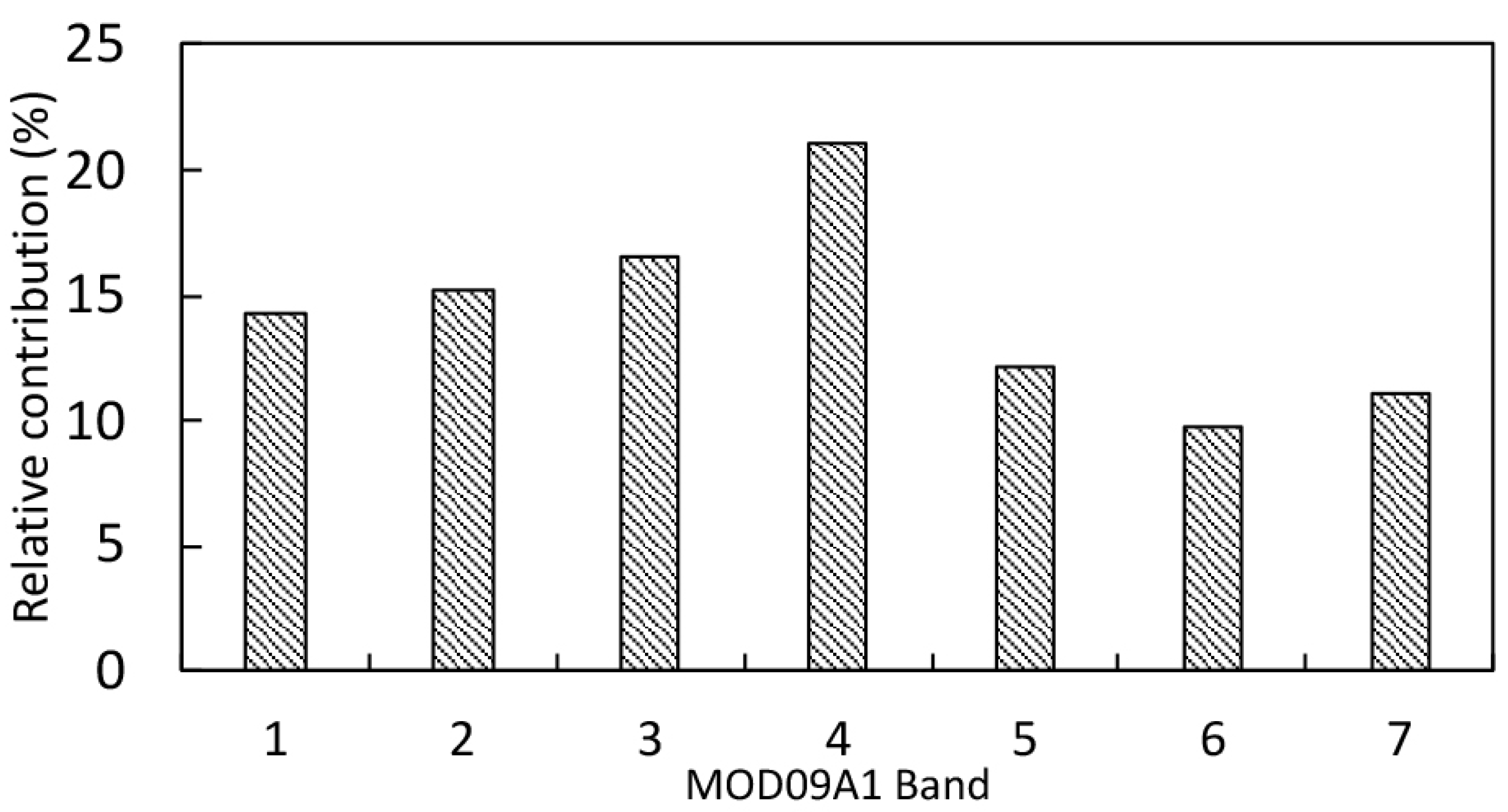
2.1. MODIS Surface Reflectance Data
2.2. MPF Measurements for Network Training
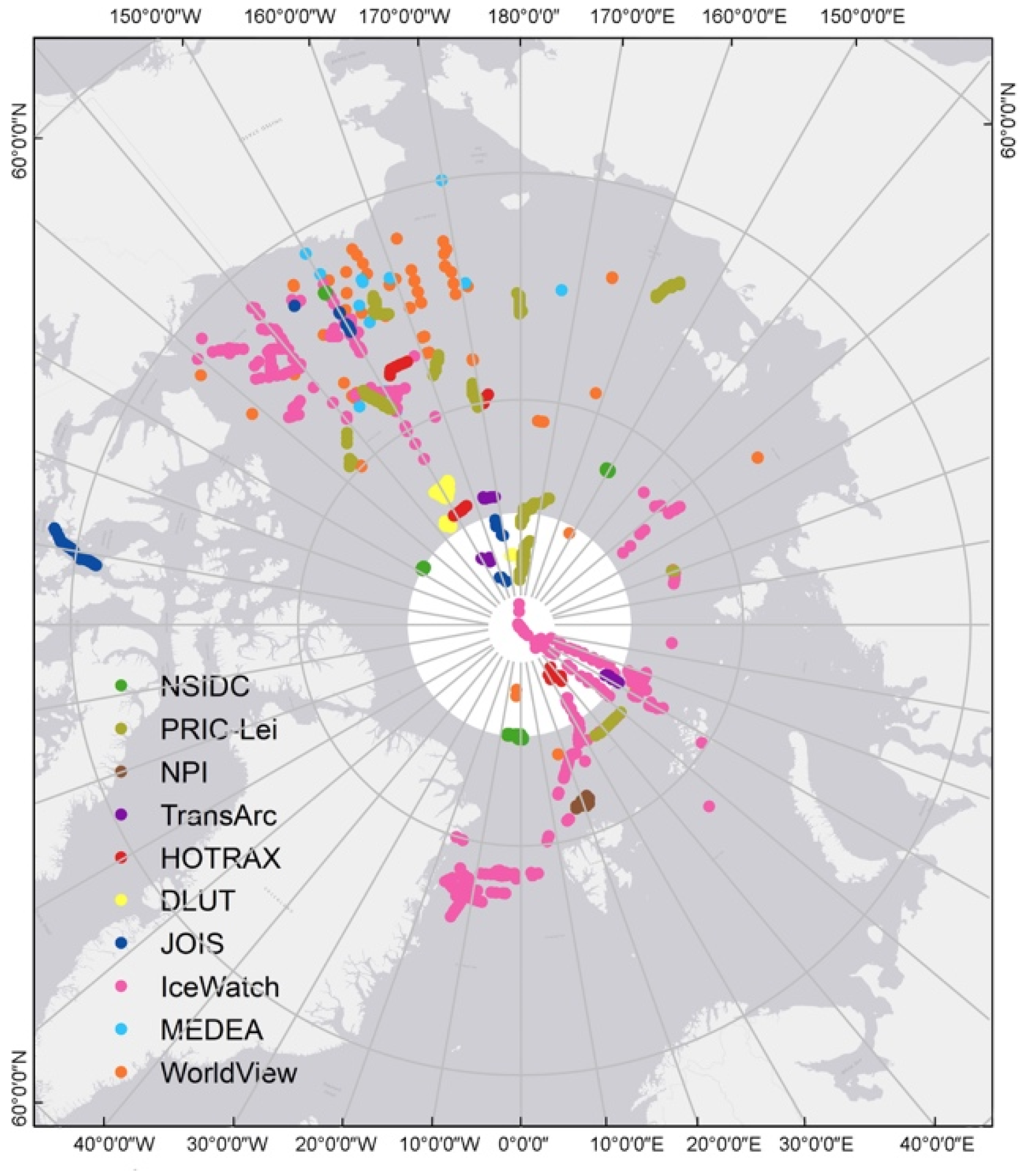
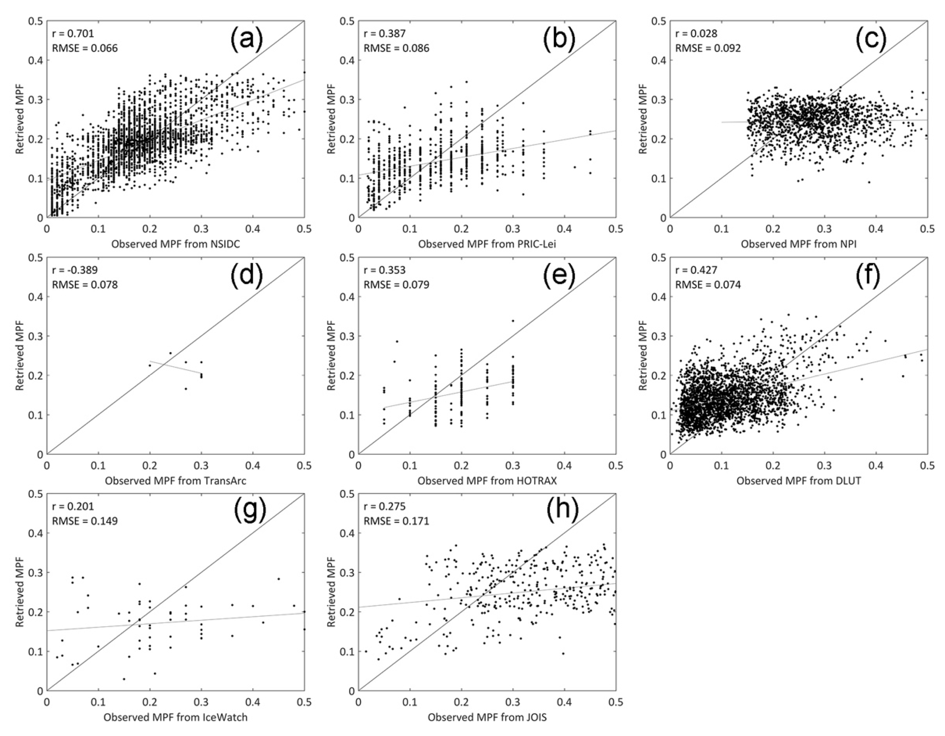
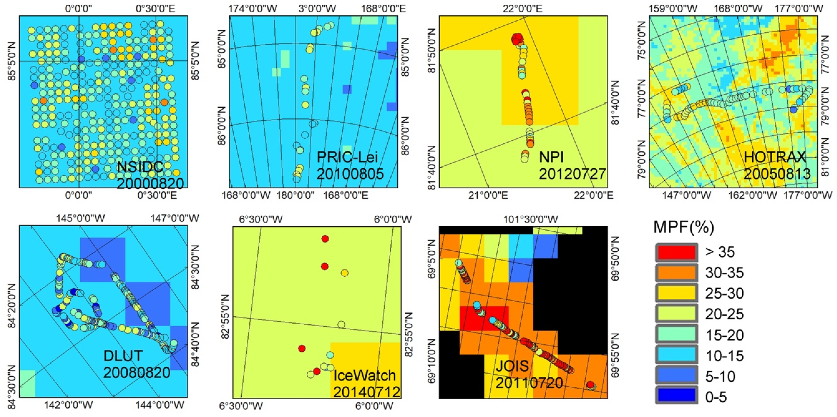
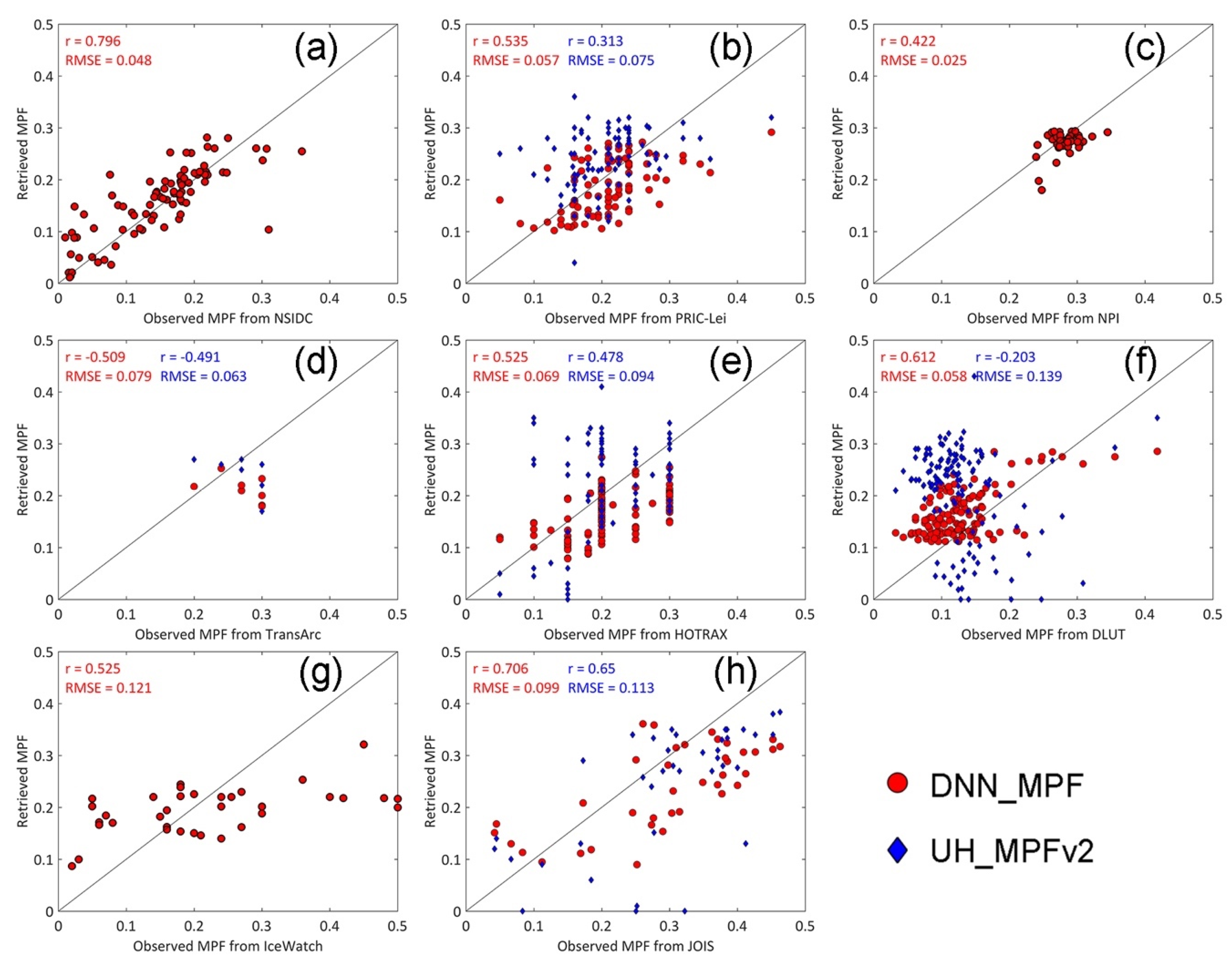
- NSIDC: The MPFs were obtained from the NSIDC during summer of 2000 and 2001 [53]. Development of this data set was based on experience gained using reconnaissance imagery during the Surface Heat Budget of the Arctic Ocean (SHEBA) and earlier summer ice monitoring experiments [54,55]. Visible band imagery was analyzed using supervised maximum likelihood classification to derive either two (water and ice) or three (pond, open water, and ice) surface classes. The estimated pond coverage was under 500 m square cells within 10 km square images (image resolution is 1 m). The NSIDC MPF used in the network training was measured at 72.8–85.1°N from June to August in 2000 and 2001. The coverage of each MPF estimation is 500 × 500 m. The measurement from NSIDC is the MPF relative to grid (the coverage of each observation). The data can be found at https://nsidc.org/data/G02159/versions/1.
- PRIC-Lei: MPFs were collected during the Arctic Research Expeditions by the Polar Research Institute of China (PRIC) in summer from 2010 to 2016 [56]. Half-hourly Arctic Shipborne Sea Ice Standardization Tool (ASSIST) observations were conducted at the bridge of the R/V Xuelong to document ice conditions, including sea ice concentration (SIC), snow thickness, fractions of melt ponds, dirty ice, ridging, and floe size. SIC was only assessed for a local area with a diameter of 1–2 km and MPF was estimated around the ship within 1 km. The MPF of PRIC-Lei used in the network training was measured along the cruise at 71.7°–88.4°N from July to September in 2010, 2012, 2014, and 2016. The coverage of each MPF record is about 1 × 1 km. The measurement from PRIC-Lei is MPF relative to ice-covered area. The data could be obtained by contacting the first author in Lei et al. [56].
- NPI: The MPFs were collected by the Norwegian Polar Institute (NPI) during the field campaign on Arctic sea ice north of Svalbard in summer 2012 [57,58]. The data set presents regional scale of about 150 km morphological properties of a relatively thin, 70–90 cm modal thickness, first-year Arctic sea ice pack in an advanced stage of melt. The data comprise fractions of three surface types (bare ice, melt ponds, and open water) along the flight tracks calculated from images acquired by a helicopter-borne camera system. The NPI MPF used in the network training was measured at 81.4–82.7°N during late July to early August in 2012. The coverage (footprint) of each MPF record is about 60 × 40 m. The obtained measurement from NPI is the MPF relative to ice-covered area. The data can be found at https://data.npolar.no/dataset/5de6b1e4-b62f-4bd4-889c-8eb7bb862d3b.
- TransArc: MPFs were collected from the ice breaker RV Polarstern during the Germany Trans-Polar cruise ARKXXVI/3 [59]. The TransArc was conducted from August to October 2011. Visual observations of sea ice conditions were performed hourly from the bridge of Polarster. Sea ice type and thickness, snow depth, pond coverage, and surface scattering layer depth were recorded during the cruise. The MPF observations were based on the ASPeCT protocol. It should be noted that the TransArc MPF was recorded on multiyear and first-year ice, respectively, for some cases, the MPF was estimated by using the linear mix of these values. The visibility in TransArc ranges between 50 m and 10 km based on ASPeCT. The TransArc MPF used in the network training was measured at 83.1°–86.3°N from August to September in 2011 and the visibility of the records ranges from 50 m to 1 km. The obtained measurement from TransArc is the MPF relative to ice-covered area. The data can be found at https://doi.pangaea.de/10.1594/PANGAEA.803312.
- HOTRAX: MPFs were collected during the Healy Oden Trans-Arctic Expedition (HOTRAX) by the Polar Science Center, University of Washington [60]. The HOTRAX was conducted from August to September 2005 to obtain physical properties of the ice pack. The ice survey was made based on ice station measurements, helicopter survey flights, and the deployment of autonomous ice mass balance buoys. The MPFs from HOTRAX used in the network training were measured at 74.4°–86.1°N from August to September 2005. The coverage of each MPF measurement is about 57 × 70 m. The obtained measurement from HOTRAX is the MPF relative to the grid (the coverage of each observation). The data could be obtained by contacting the first author in Perovich et al. [60].
- DLUT: MPFs were collected during two Chinese Arctic Research Expeditions by the Dalian University of Technology (DLUT) [26,61]. The first survey of DLUT was conducted from July to September 2008 during the third Chinese Arctic Research Expedition. During the cruise, eight helicopter flights were conducted, and more than 9000 aerial images were obtained in the Pacific sector of the Arctic. Each image covers an area of approximately 98 × 67 m [61]. The second survey of DLUT was conducted from July to September 2010 using underway ship- and helicopter-based ice observations. The images were classified into three surface categories (sea ice/snow, water, and melt ponds). The flight altitude varied between 150 and 500 m. Each image covers an area between 147 × 100 m and 490 × 335 m [26]. The images from the two cruises are spaced without overlapping, and each image represents an independent scene. The DLUT MPF used in the network training was measured at 71.9°–81.0°N during August to September 2008 and July to September 2010. The coverage of each MPF estimated from the airborne image is about 98 × 67 m or ranges from 147 × 100 m to 490 × 335 m. The obtained measurement from DLUT is the MPF relative to the grid (image area). The data could be obtained by contacting the first author in Lu et al. [61] and Huang et al. [26].
- IceWatch: The MPFs were collected from the IceWatch community. Ice Watch is a program coordinating visual observations of sea ice conducted from ships in the northern hemisphere. Several parameters related to ice conditions are recorded using the ASSIST tool, including ice types, SIC, snow depth, MPF, melt pond depth. The MPF used in the network training was measured at 71.4°–89.9°N from several cruises during August to September 2012, August 2013, July to September 2014, August 2015, and July to August 2018. The visibility of the observations ranges from 50 m to 10 km. Here we only use the observations with visibility below 1 km in the network training. The obtained measurement from IceWatch is the MPF relative to ice-covered area. The data can be found at https://icewatch.met.no/.
- JOIS: The MPFs were collected from the ship-based observations by Joint Ocean Ice Study (JOIS). The JOIS was conducted during 2003–2014 on the Canadian Coast Guard Ship Louis S. St-Laurent [44]. The cameras were mounted with a view of the horizon and ice pack in front of the ship. The images were classified into five types (water only; ice only; water and ice; pond and ice; water, pond, and ice). Due to the camera malfunction and some bad ice conditions, information was missing in some years [44]. The MPF used in the network training was measured at 68.9–88.2°N during July to September 2011. The covered areas of per image range from 1453 to 2397 m2. The obtained measurement from JOIS is the MPF relative to the grid (image area). The data could be obtained by contacting the first author in Tanaka et al. [44].
2.3. MPF Measurements for Independent Validation
- MEDEA: The MPFs were retrieved by the Polar Science Center, University of Washington based on the classified high-resolution (1 m resolution) visible band satellite images following Webster et al. [8]. The MPFs were measured at 69–86.5°N over the Beaufort Sea, Chukchi Sea, the Canadian Arctic, the Fram Strait, and the East Siberian Sea from May to August for the period of 1999–2014. The scene size (square grid) of the MPFs ranges from 5 to 25 km. In validation, we used the observations from June to August during 2000–2011. The obtained measurement from MEDEA is the MPF relative to ice-covered area. In validation, the MPF was transferred to the fraction relative to the grid (image area) using the measured SIC from MEDEA. The data can be found at http://psc.apl.uw.edu/melt-pond-data/.
- WorldView: The MPFs were collected from the WorldView satellite imagery during 2010–2015 by Wright and Polashenski [63]. The high resolution (0.46 and 1.84 m resolution) WorldView optical satellite imagery is able to capture the evolution of the ice and ocean surface state directly [45]. This dataset contains the results from processing the WorldView imagery of sea ice using an Open Source Sea-Ice Processing algorithm [45]. This method classifies surface coverage into three main categories: snow and bare ice; melt ponds and submerged ice; open water. Tests show the classification accuracy of this method typically exceeds 96% [45]. The recorded data covers from March to August during 2010–2015. The coverage of the WorldView imagery ranges from 77 to 728 km2. In validation, we used the observations from May to August during 2010–2015. The obtained measurement from WorldView is the MPF relative to the grid (image area). The data can be found at https://arcticdata.io/catalog/view/doi:10.18739/A22Z12P4J.
2.4. Method
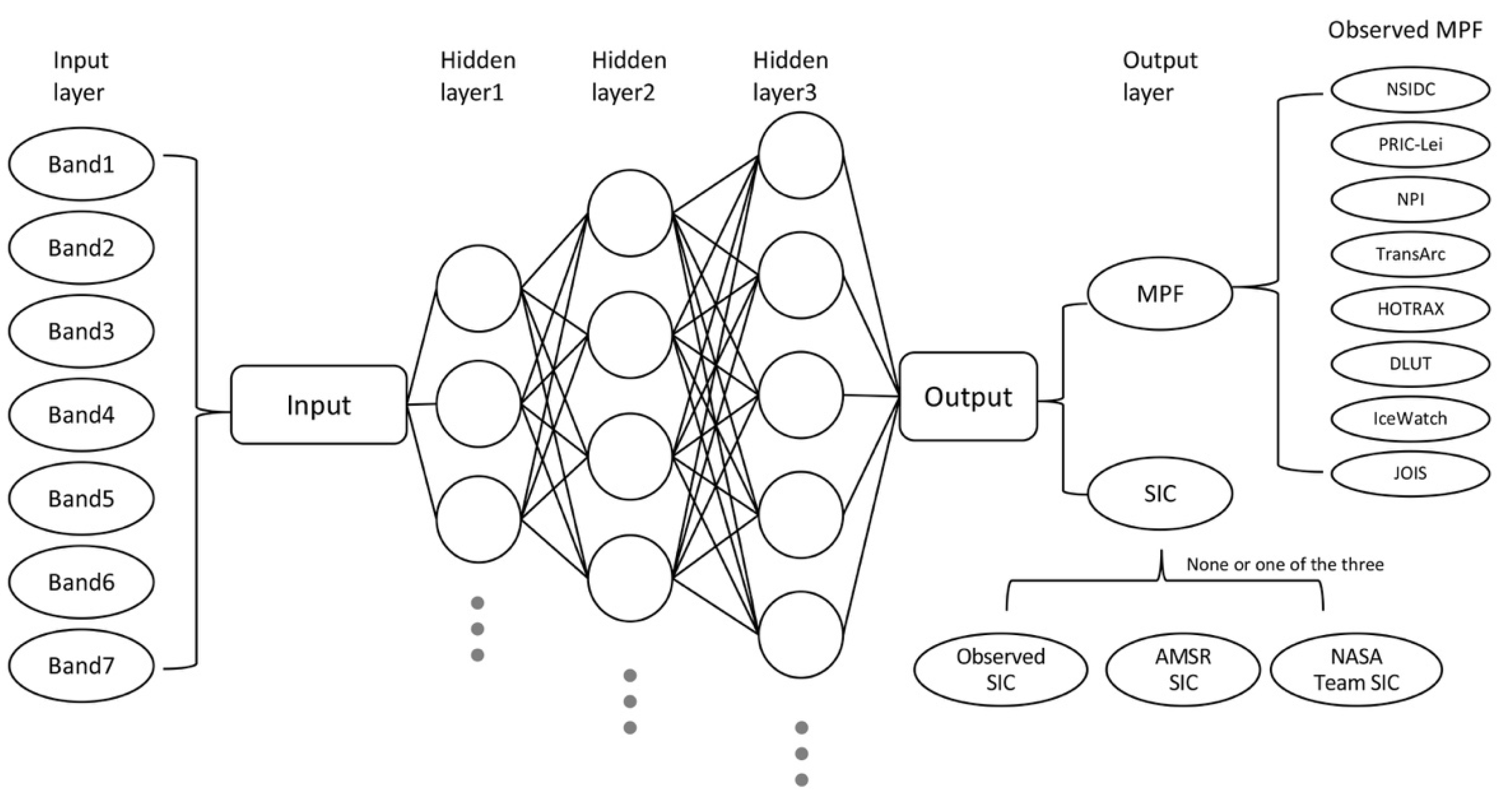
2.4.1. Ensemble-Based Deep Neural Network
- DNN_MPF (no SIC) is the DNN trained only using the processed MPF from the observations in Section 2.2 as the target data. The DNN_MPF (no SIC) does not include SIC as the target.
- DNN_MPF+ ObsSIC is the DNN trained by adding the processed SIC from the observations in Section 2.2 as the second target. The observed MPF and SIC are from the same source.
- DNN_MPF+AMSRSIC is the DNN trained by adding the SIC derived from the Advanced Microwave Scanning Radiometer-Earth Observing System and Advanced Microwave Scanning Radiometer 2 (referred to as AMSR SIC [64]) as the second target. The AMSR SIC is developed by the University of Bremen using the ARTIST Sea Ice algorithm. In the DNN training, the AMSR SIC was resampled from 6.25 km to the 500 m polar stereographic grid and then extracted based on the latitude and longitude of the corresponding MPF observation. The SIC data can be found at https://seaice.uni-bremen.de/sea-ice-concentration.
- DNN_MPF+NASASIC is the DNN trained by adding the SIC derived from the Nimbus-7 SMMR and DMSP SSM/I-SSMIS Passive Microwave Data based on a NASA Team algorithm (referred to as NASA Team SIC [62]) as the second target. In the DNN training, the NASA Team SIC is resampled from 25 km to the 500 m polar stereographic grid and then extracted based on the latitude and longitude of the corresponding MPF observation. The SIC data can be found at https://nsidc.org/data/nsidc-0051.
2.4.2. Retrieval of the Final MPF Dataset
3. Results
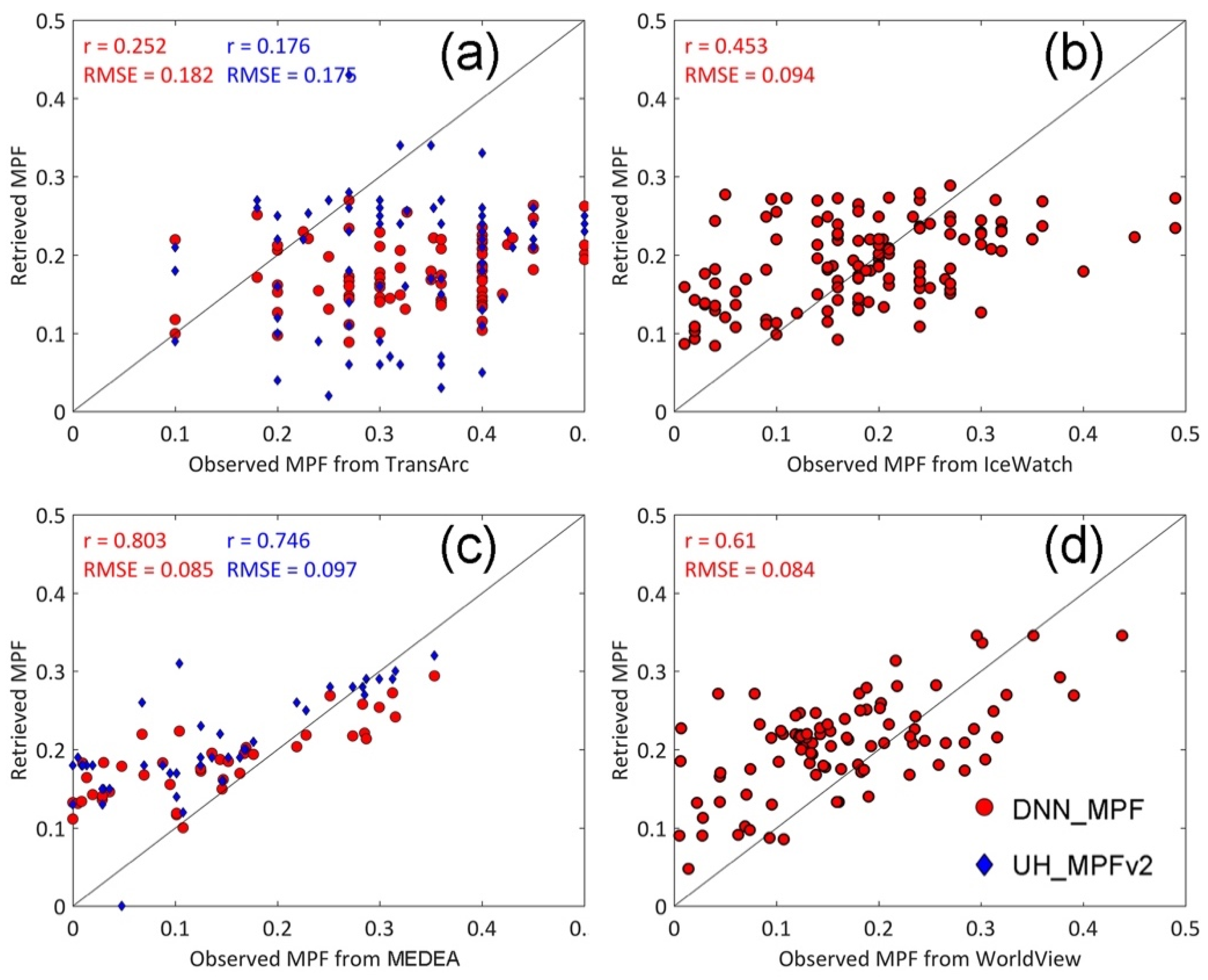
3.1. Evaluation
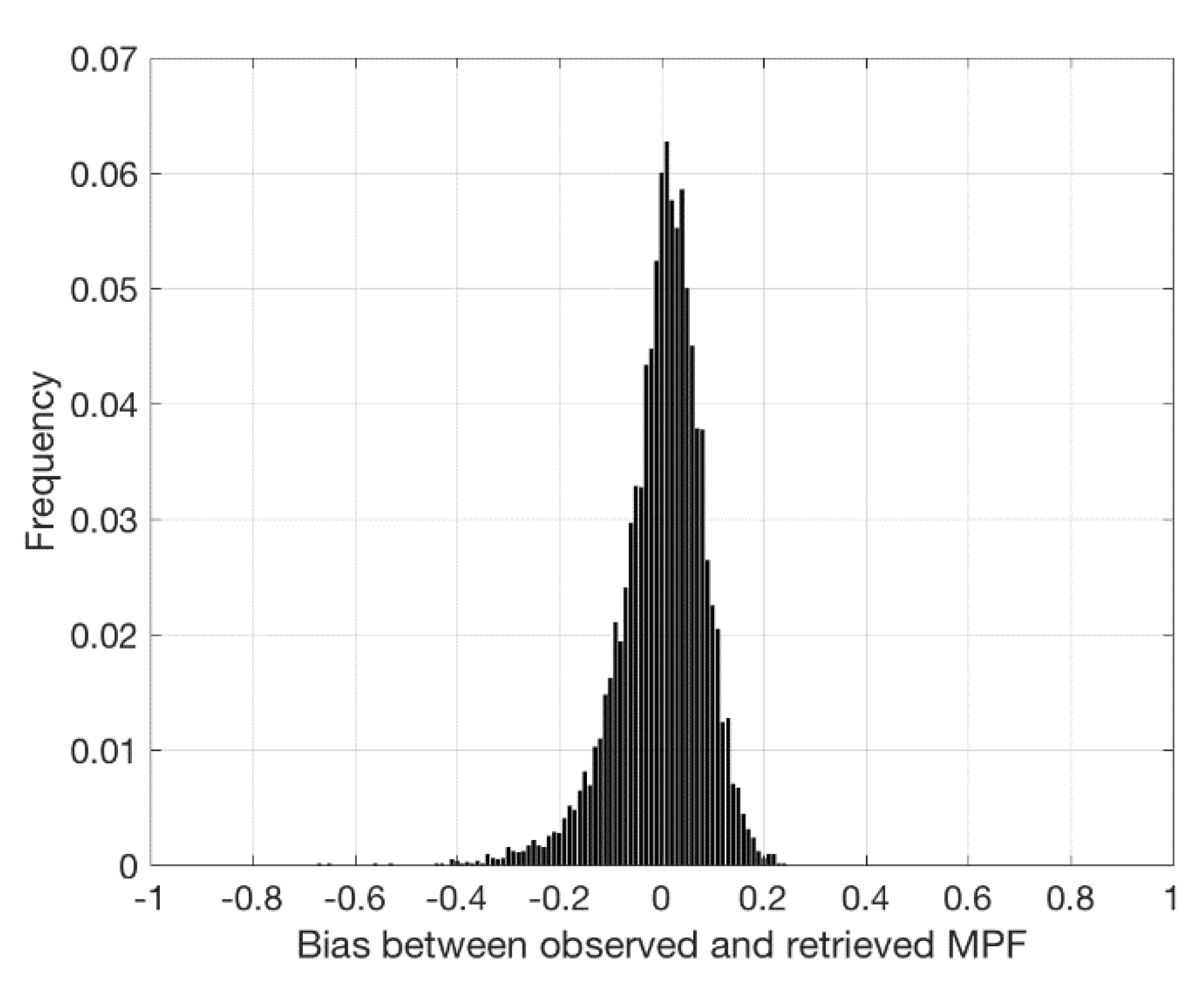
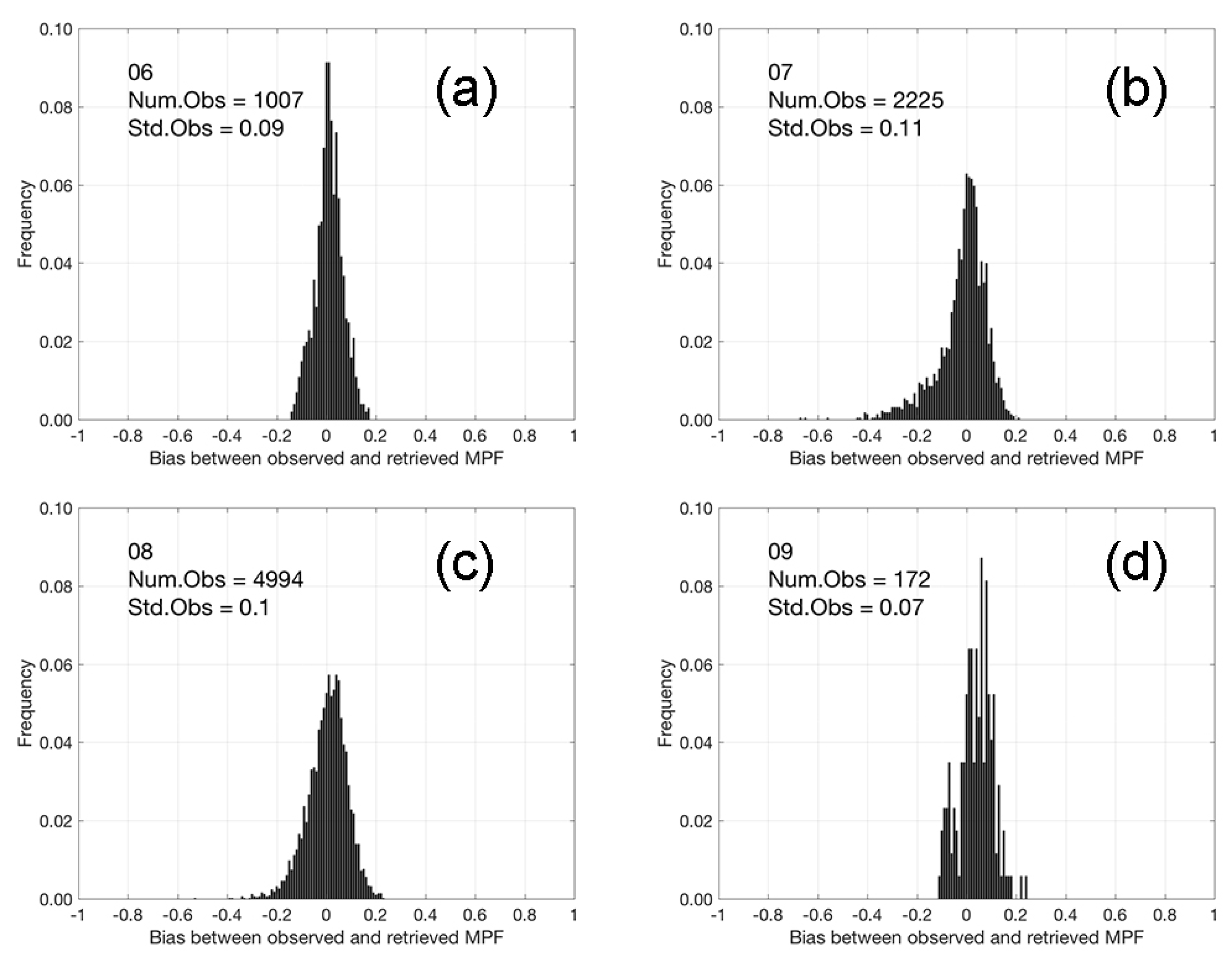
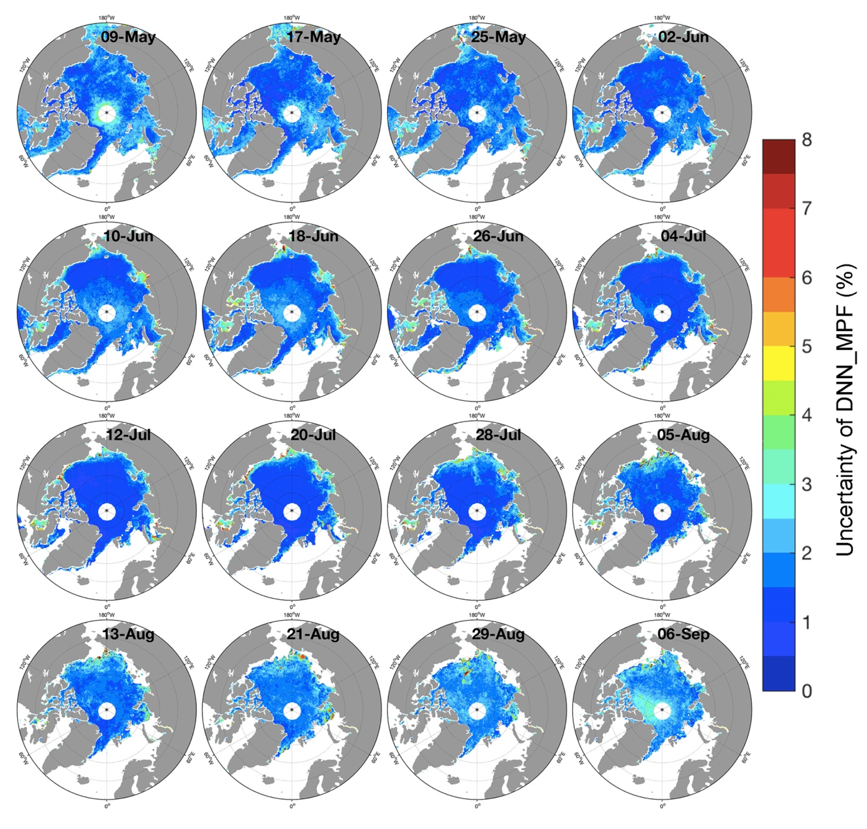
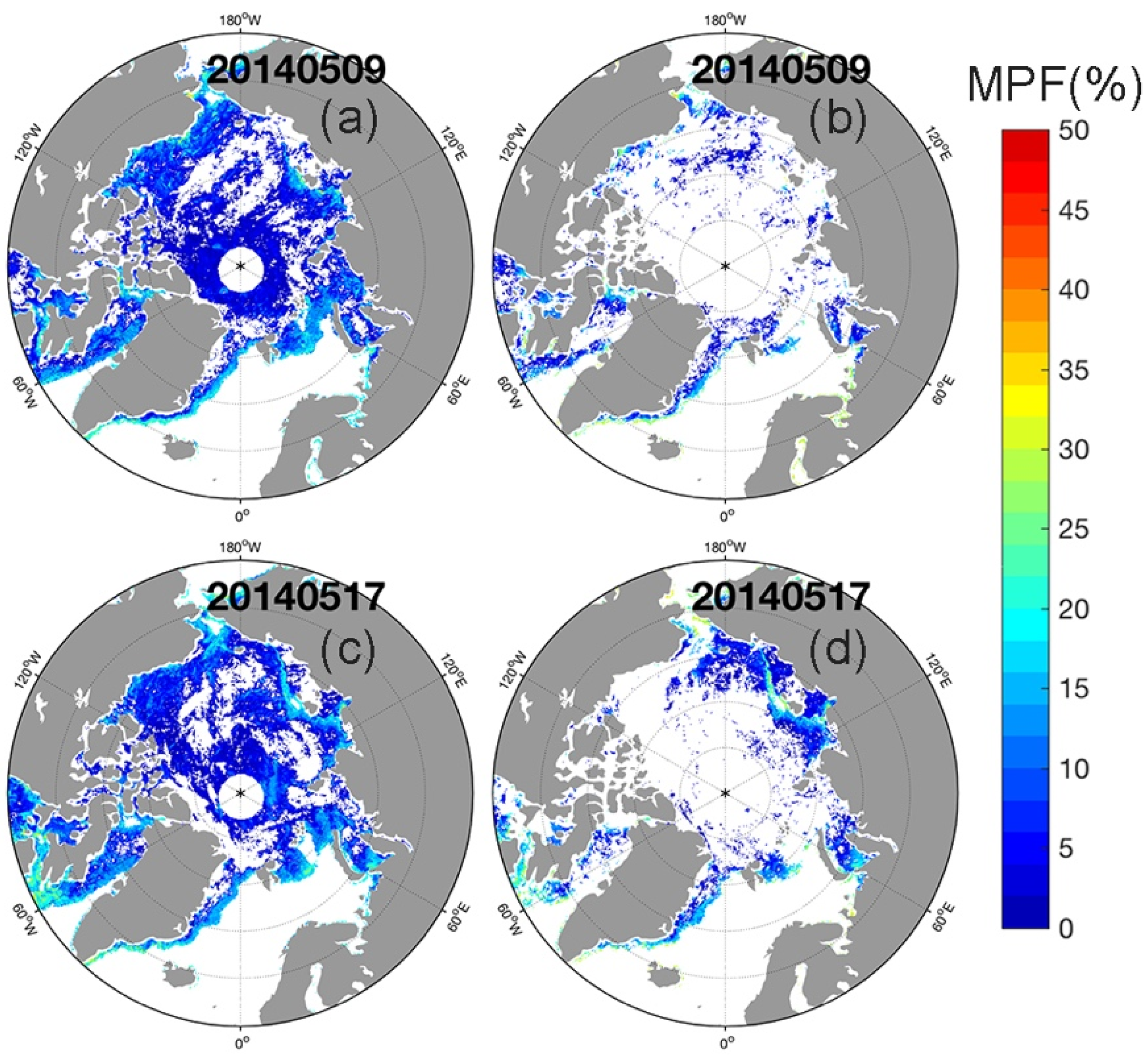
3.2. Uncertainties
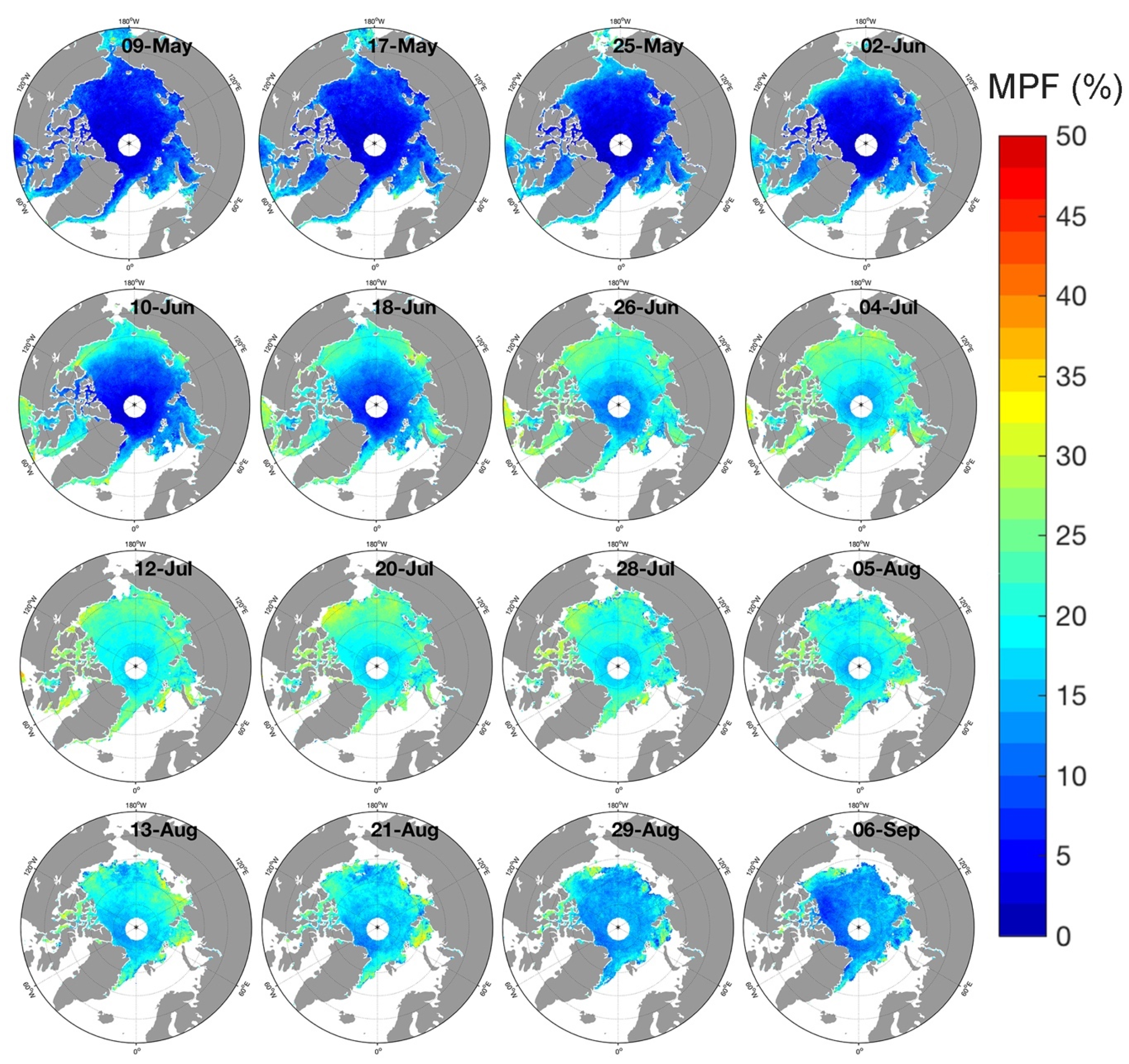
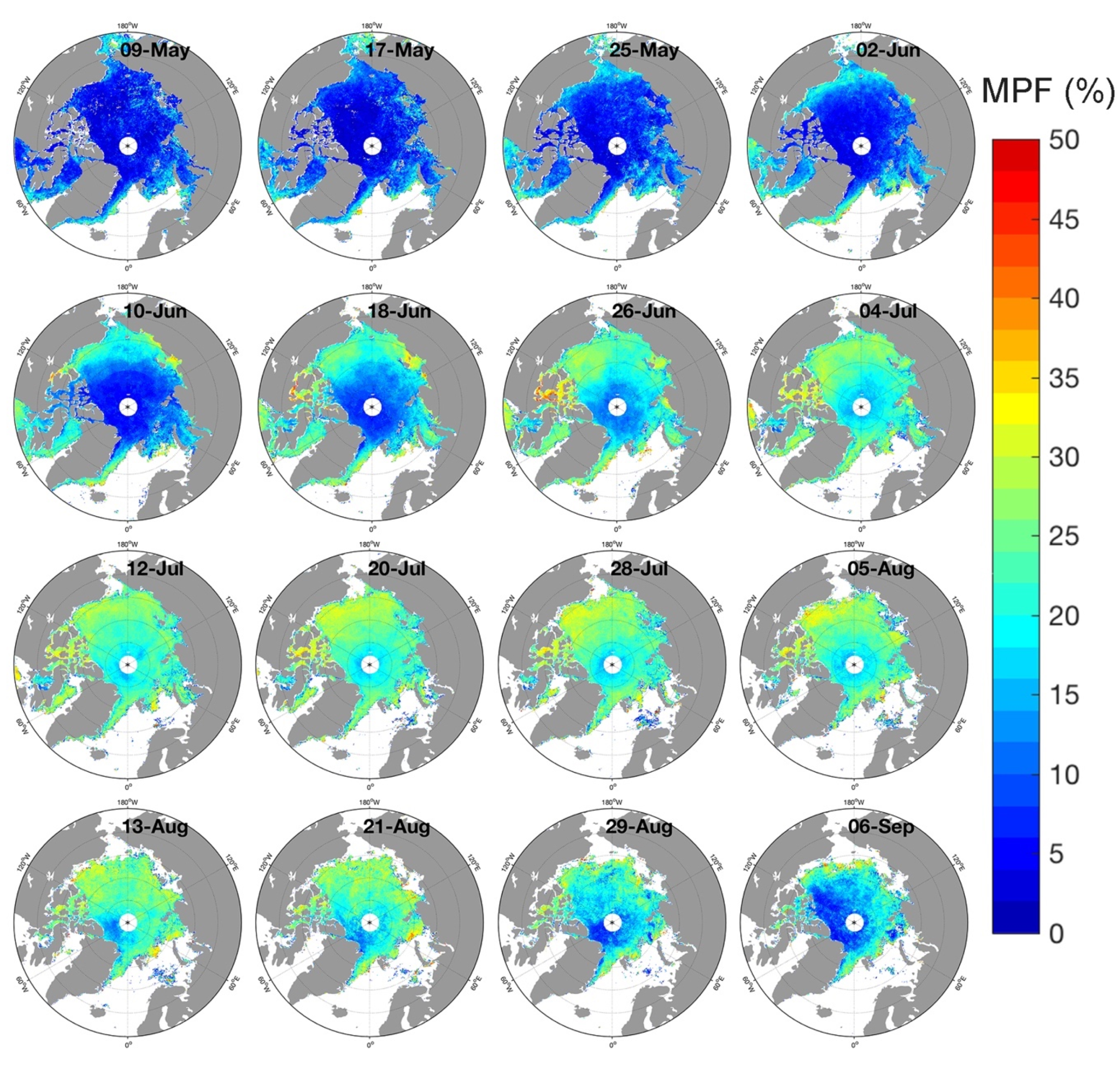
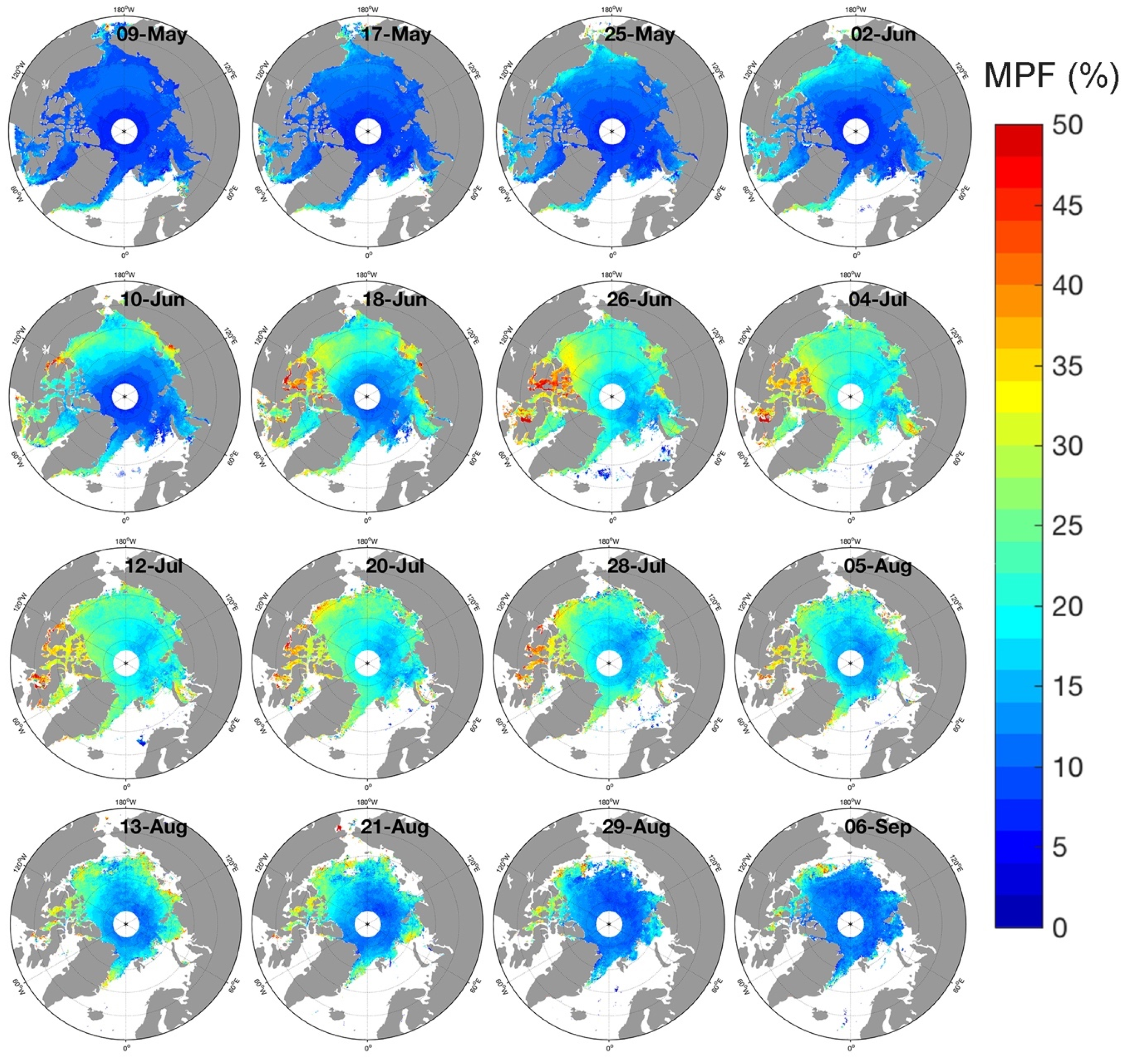
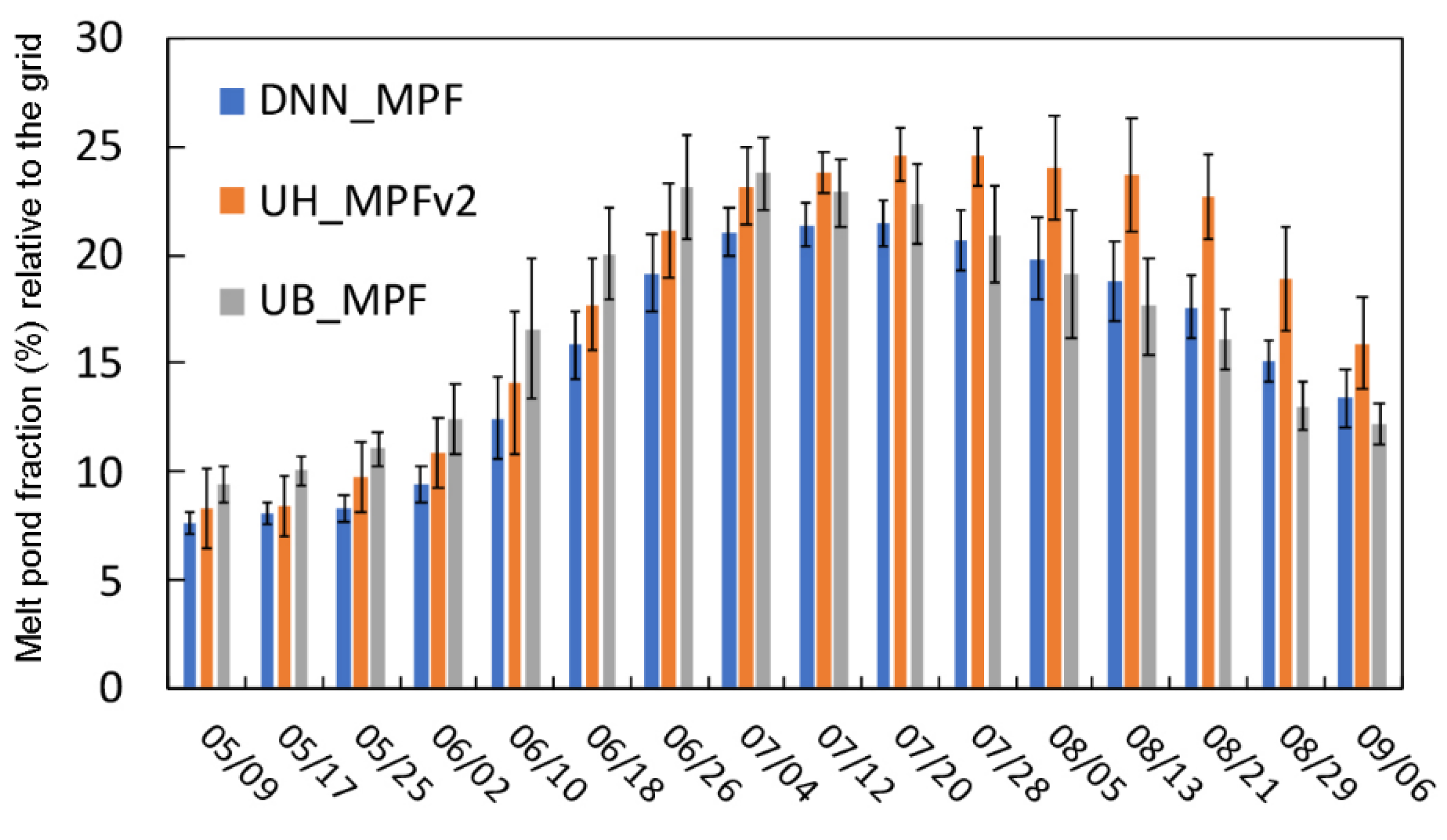
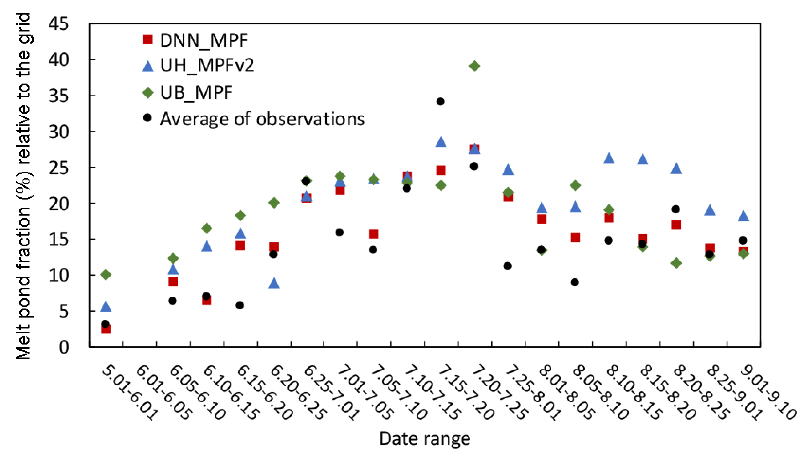
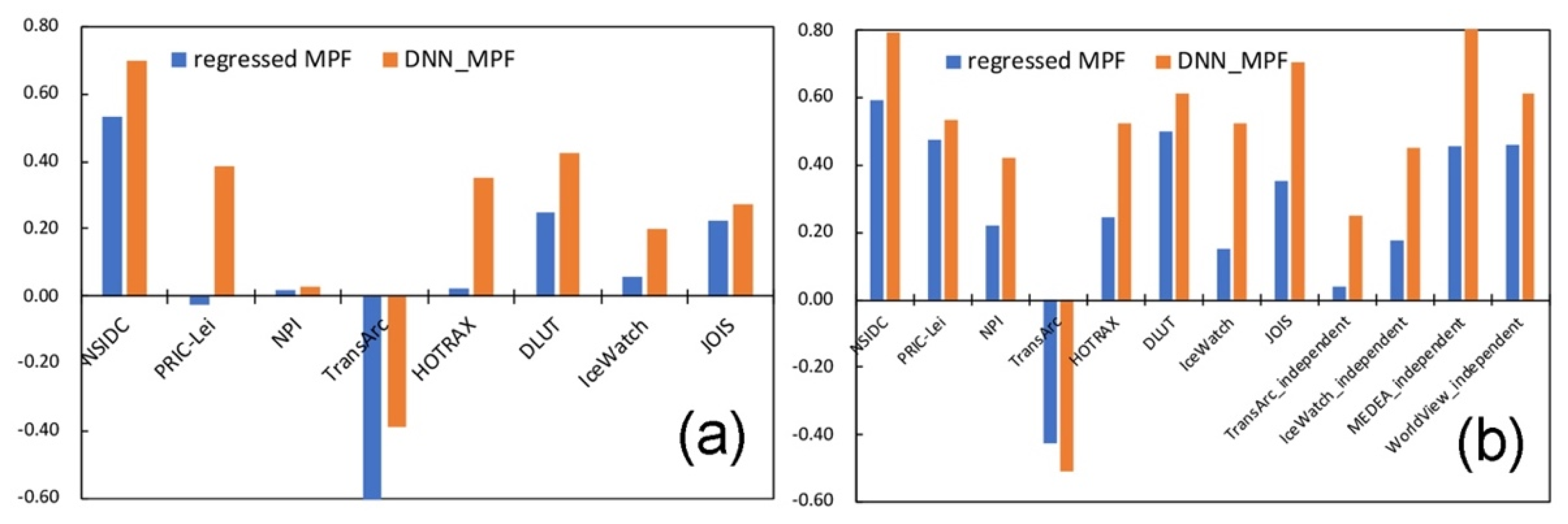
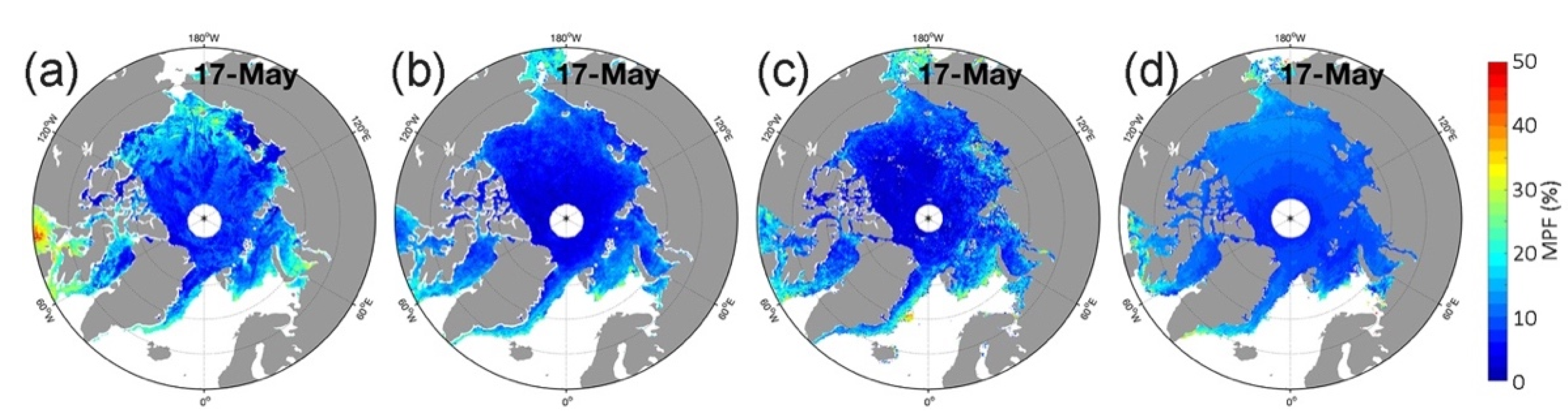
3.3. Inter-Comparison
4. Discussion
5. Conclusions
Supplementary Materials
Author Contributions
Funding
Acknowledgments
Conflicts of Interest
References
- Yackel, J.J.; Barber, D.G.; Hanesiak, J.M. Melt ponds on sea ice in the Canadian Archipelago: 1. Variability in morphological and radiative properties. J. Geophys. Res. Oceans 2000, 105, 22049–22060. [Google Scholar] [CrossRef]
- Sturm, M.; Holmgren, J.; Perovich, D.K. Winter snow cover on the sea ice of the Arctic Ocean at the Surface Heat Budget of the Arctic Ocean (SHEBA): Temporal evolution and spatial variability. J. Geophys. Res. Oceans 2002, 107, 8047. [Google Scholar] [CrossRef]
- Eicken, H.; Grenfell, T.C.; Perovich, D.K.; Richter-Menge, J.A.; Frey, K. Hydraulic controls of summer Arctic pack ice albedo. J. Geophys. Res. Oceans 2004, 109, C08007. [Google Scholar] [CrossRef] [Green Version]
- Perovich, D.K.; Polashenski, C. Albedo evolution of seasonal Arctic sea ice. Geophys. Res. Lett. 2012, 39, L08501. [Google Scholar] [CrossRef]
- Polashenski, C.; Perovich, D.; Courville, Z. The mechanisms of sea ice melt ponds formation and evolution. J. Geophys. Res. Oceans 2012, 117, C01001. [Google Scholar] [CrossRef]
- Tschudi, M.A.; Curry, J.A.; Maslanik, J.A. Airborne observations of summertime surface features and their effect on surface albedo during FIRE/SHEBA. J. Geophys. Res. Atmos. 2001, 106, 15335–15344. [Google Scholar] [CrossRef]
- Perovich, D.K.; Grenfell, T.C.; Light, B.; Hobbs, P.V. Seasonal evolution of the albedo of multiyear Arctic sea ice. J. Geophys. Res. Oceans 2002, 107, 8044. [Google Scholar] [CrossRef]
- Webster, M.A.; Rigor, I.G.; Perovich, D.K.; Richter-Menge, J.A.; Polashenski, C.M.; Light, B. Seasonal evolution of melt ponds on Arctic sea ice. J. Geophys. Res. Oceans 2015, 120, 5968–5982. [Google Scholar] [CrossRef]
- Curry, J.A.; Schramm, J.L.; Ebert, E.E. Sea ice-albedo climate feedback mechanism. J. Clim. 1995, 8, 240–247. [Google Scholar] [CrossRef]
- Perovich, D.K.; Tucker, W.B. Arctic sea-ice conditions and the distribution of solar radiation during summer. Ann. Glaciol. 1997, 25, 445–450. [Google Scholar] [CrossRef] [Green Version]
- Perovich, D.K.; Light, B.; Eicken, H.; Jones, K.F.; Runciman, K.; Nghiem, S.V. Increasing solar heating of the Arctic Ocean and adjacent seas, 1979–2005: Attribution and role in the ice-albedo feedback. Geophys. Res. Lett. 2007, 34, L19505. [Google Scholar] [CrossRef] [Green Version]
- Anderson, M.R.; Drobot, S.D. Spatial and temporal variability in snowmelt onset over Arctic sea ice. Ann. Glaciol. 2001, 33, 74–78. [Google Scholar] [CrossRef] [Green Version]
- Perovich, D.K.; Nghiem, S.V.; Markus, T.; Schweiger, A. Seasonal evolution and interannual variability of the local solar energy absorbed by the Arctic sea ice–ocean system. J. Geophys. Res. Oceans 2007, 112, C03005. [Google Scholar] [CrossRef]
- Tschudi, M.A.; Maslanik, J.A.; Perovich, D.K. Derivation of melt ponds coverage on Arctic sea ice using MODIS observations. Remote Sens. Environ. 2008, 112, 2605–2614. [Google Scholar] [CrossRef]
- Holland, M.M.; Bailey, D.A.; Briegleb, B.P.; Light, B.; Hunke, E. Improved sea ice shortwave radiation physics in CCSM4: The impact of melt ponds and aerosols on Arctic sea ice. J. Clim. 2012, 25, 1413–1430. [Google Scholar] [CrossRef]
- Nicolaus, M.; Katlein, C.; Maslanik, J.; Hendricks, S. Changes in Arctic sea ice result in increasing light transmittance and absorption. Geophys. Res. Lett. 2012, 39, L24501. [Google Scholar] [CrossRef] [Green Version]
- Nicolaus, M.; Katlein, C.; Maslanik, J.; Hendricks, S. Correction to “Changes in Arctic sea ice result in increasing light transmittance and absorption”. Geophys. Res. Lett. 2013, 40, 2699–2700. [Google Scholar] [CrossRef] [Green Version]
- Arrigo, K.R.; Perovich, D.K.; Pickart, R.S.; Brown, Z.W.; Van Dijken, G.L.; Lowry, K.E.; Bates, N.R. Massive phytoplankton blooms under Arctic sea ice. Science 2012, 1215065. [Google Scholar] [CrossRef] [Green Version]
- Palmer, M.A.; Saenz, B.T.; Arrigo, K.R. Impacts of sea ice retreat, thinning, and melt-pond proliferation on the summer phytoplankton bloom in the Chukchi Sea, Arctic Ocean. Deep Sea Res. Part II 2014, 105, 85–104. [Google Scholar] [CrossRef]
- Arctic Climate Impact Assessment (ACIA). Impacts of a Warming Arctic; Cambridge University Press: Cambridge, UK, 2004; 140p. [Google Scholar]
- Serreze, M.C.; Francis, J.A. The Arctic amplification debate. Clim. Chang. 2006, 76, 241–264. [Google Scholar] [CrossRef] [Green Version]
- IPCC. Summary for Policymakers. In Climate Change 2013. The Physical Science Basis, Contribution of Working Group I to the Fifth Assessment Report of the Intergovernmental Panel on Climate Change; Cambridge University Press: Cambridge, UK, 2013. [Google Scholar]
- Stroeve, J.C.; Serreze, M.C.; Holland, M.M.; Kay, J.E.; Malanik, J.; Barrett, A.P. The Arctic’s rapidly shrinking sea ice cover: A research synthesis. Clim. Chang. 2012, 110, 1005–1027. [Google Scholar] [CrossRef] [Green Version]
- Comiso, J.C.; Parkinson, C.L.; Gersten, R.; Stock, L. Accelerated decline in the Arctic sea ice cover. Geophys. Res. Lett. 2008, 35, L01703. [Google Scholar] [CrossRef] [Green Version]
- Serreze, M.C.; Stroeve, J. Arctic sea ice trends, variability and implications for seasonal ice forecasting. Philos. Trans. R. Soc. A Math. Phys. Eng. Sci. 2015, 373, 20140159. [Google Scholar] [CrossRef] [PubMed] [Green Version]
- Huang, W.; Lu, P.; Lei, R.; Xie, H.; Li, Z. Melt pond distribution and geometry in high Arctic sea ice derived from aerial investigations. Ann. Glaciol. 2016, 57, 105–118. [Google Scholar] [CrossRef] [Green Version]
- Hutchings, J.K.; Faber, M.K. Sea-Ice Morphology Change in the Canada Basin Summer: 2006–2015 Ship Observations Compared to Observations From the 1960s to the Early 1990s. Front. Earth Sci. 2018, 6, 123. [Google Scholar] [CrossRef] [Green Version]
- Rösel, A.; Kaleschke, L. Exceptional melt pond occurrence in the years 2007 and 2011 on the Arctic sea ice revealed from MODIS satellite data. J. Geophys. Res. Oceans 2012, 117. [Google Scholar] [CrossRef]
- Schröder, D.; Feltham, D.L.; Flocco, D.; Tsamados, M. September Arctic sea-ice minimum predicted by spring melt-pond fraction. Nat. Clim. Chang. 2014, 4, 353–357. [Google Scholar] [CrossRef]
- Liu, J.; Song, M.; Horton, R.M.; Hu, Y. Revisiting the potential of melt ponds fraction as a predictor for the seasonal Arctic sea ice extent minimum. Environ. Res. Lett. 2015, 10, 054017. [Google Scholar] [CrossRef] [Green Version]
- Markus, T.; Cavalieri, D.J.; Ivanoff, A. The potential of using Landsat 7 ETM+ for the classification of sea-ice surface conditions during summer. Ann. Glaciol. 2002, 34, 415–419. [Google Scholar] [CrossRef] [Green Version]
- Markus, T.; Cavalieri, D.J.; Tschudi, M.A.; Ivanoff, A. Comparison of aerial video and Landsat 7 data over ponded sea ice. Remote Sens. Environ. 2003, 86, 458–469. [Google Scholar] [CrossRef]
- Rösel, A.; Kaleschke, L.; Birnbaum, G. Melt ponds on Arctic sea ice determined from MODIS satellite data using an artificial neural network. Cryosphere 2012, 6, 431–446. [Google Scholar] [CrossRef] [Green Version]
- Wright, N.C.; Polashenski, C.M. How machine learning and high—Resolution imagery can improve melt pond retrieval from MODIS over current spectral unmixing techniques. J. Geophys. Res. Oceans 2020, e2019JC015569. [Google Scholar] [CrossRef]
- Rösel, A.; Kaleschke, L.; Kern, S. Gridded Melt Pond Cover Fraction on Arctic Sea Ice Derived from TERRA-MODIS 8-Day Composite Reflectance Data Bias Corrected Version 02; World Data Center for Climate (WDCC) at DKRZ: Hamburg, Germany, 2015. [Google Scholar] [CrossRef]
- Istomina, L.; Heygster, G.; Huntemann, M.; Schwarz, P.; Birnbaum, G.; Scharien, R.; Polashenski, C.; Perovich, D.; Zege, E.; Malinka, A.; et al. Melt ponds fraction and spectral sea ice albedo retrieval from MERIS data-Part 1: Validation against in situ, aerial, and ship cruise data. Cryosphere 2015, 9, 1551–1566. [Google Scholar] [CrossRef] [Green Version]
- Zege, E.; Malinka, A.; Katsev, I.; Prikhach, A.; Heygster, G.; Istomina, L.; Birnbaum, G.; Schwarz, P. Algorithm to retrieve the melt ponds fraction and the spectral albedo of Arctic summer ice from satellite optical data. Remote Sens. Environ. 2015, 163, 153–164. [Google Scholar] [CrossRef] [Green Version]
- Kim, D.J.; Hwang, B.; Chung, K.H.; Lee, S.H.; Jung, H.S.; Moon, W.M. Melt ponds mapping with high-resolution SAR: The first view. Proc. IEEE 2013, 101, 748–758. [Google Scholar] [CrossRef]
- Scharien, R.K.; Hochheim, K.; Landy, J.; Barber, D.G. First-year sea ice melt ponds fraction estimation from dual-polarisation C-band SAR—Part 2: Scaling in situ to Radarsat-2. Cryosphere 2014, 8, 2163–2176. [Google Scholar] [CrossRef] [Green Version]
- Scharien, R.K.; Landy, J.; Barber, D.G. First-year sea ice melt ponds fraction estimation from dual-polarisation C-band SAR—Part 1: In situ observations. Cryosphere 2014, 8, 2147–2162. [Google Scholar] [CrossRef] [Green Version]
- Mäkynen, M.; Kern, S.; Rösel, A.; Pedersen, L.T. On the estimation of melt ponds fraction on the Arctic Sea ice with ENVISAT WSM images. IEEE Trans. Geosci. Remote Sens. 2014, 52, 7366–7379. [Google Scholar] [CrossRef]
- Han, H.; Im, J.; Kim, M.; Sim, S.; Kim, J.; Kim, D.J.; Kang, S.H. Retrieval of melt ponds on arctic multiyear sea ice in summer from terrasar-x dual-polarization data using machine learning approaches: A case study in the chukchi sea with mid-incidence angle data. Remote Sens. 2016, 8, 57. [Google Scholar] [CrossRef] [Green Version]
- Li, H.; Perrie, W.; Li, Q.; Hou, Y. Estimation of melt ponds fractions on first year sea ice using compact polarization SAR. J. Geophys. Res. Oceans 2017, 122, 8145–8166. [Google Scholar] [CrossRef]
- Tanaka, Y.; Tateyama, K.; Kameda, T.; Hutchings, J.K. Estimation of melt ponds fraction over high-concentration Arctic sea ice using AMSR-E passive microwave data. J. Geophys. Res. Oceans 2016, 121, 7056–7072. [Google Scholar] [CrossRef]
- Wright, N.C.; Polashenski, C.M. Open-source algorithm for detecting sea ice surface features in high-resolution optical imagery. Cryosphere 2018, 12, 1307–1329. [Google Scholar] [CrossRef] [Green Version]
- Chang, D.H.; Islam, S. Estimation of soil physical properties using remote sensing and artificial neural network. Remote Sens. Environ. 2000, 74, 534–544. [Google Scholar] [CrossRef]
- Hong, Y.; Hsu, K.L.; Sorooshian, S.; Gao, X. Precipitation estimation from remotely sensed imagery using an artificial neural network cloud classification system. J. Appl. Meteorol. 2004, 43, 1834–1853. [Google Scholar] [CrossRef] [Green Version]
- Yu, X.; Wu, X.; Luo, C.; Ren, P. Deep learning in remote sensing scene classification: A data augmentation enhanced convolutional neural network framework. GISci. Remote Sens. 2017, 54, 741–758. [Google Scholar] [CrossRef] [Green Version]
- Liu, Q.; Zhang, Y.; Lv, Q.; Shang, L. Applying High-Resolution Visible Imagery to Satellite Melt ponds Fraction Retrieval: A Neural Network Approach. arXiv 2017, arXiv:1704.04281. [Google Scholar] [CrossRef]
- Lee, S.; Stroeve, J.; Tsamados, M.; Khan, A.L. Machine learning approaches to retrieve pan-Arctic melt ponds from visible satellite imagery. Remote Sens. Environ. 2020, 247, 111919. [Google Scholar] [CrossRef]
- Liu, J.; Zhang, Y.; Cheng, X.; Hu, Y. Retrieval of Snow Depth over Arctic Sea Ice Using a Deep Neural Network. Remote Sens. 2019, 11, 2864. [Google Scholar] [CrossRef] [Green Version]
- Vermote, E. MOD09A1 MODIS/Terra Surface Reflectance 8-Day L3 Global 500 m SIN Grid V006; NASA EOSDIS LP DAAC: Washington, DC, USA, 2015. [Google Scholar] [CrossRef]
- Fetterer, F.; Wilds, S.; Sloan, J. Arctic Sea Ice Melt Ponds Statistics and Maps, 1999–2001, Version 1; NSIDC: National Snow and Ice Data Center: Boulder, CO, USA, 2018. [Google Scholar] [CrossRef]
- NSIDC. SHEBA Reconnaissance Imagery, Version 1.0; National Snow and Ice Data Center: Boulder, CO, USA, 2000. [Google Scholar]
- Fetterer, F.; Untersteiner, N. Observations of Melt Ponds on Arctic Sea Ice. J. Geophys. Res. 1998, 103, 24821–24835. [Google Scholar] [CrossRef]
- Lei, R.; Tian-Kunze, X.; Li, B.; Heil, P.; Wang, J.; Zeng, J.; Tian, Z. Characterization of summer Arctic sea ice morphology in the 135°–175° W sector using multi-scale methods. Cold Reg. Sci. Technol. 2017, 133, 108–120. [Google Scholar] [CrossRef]
- Divine, D.V.; Granskog, M.A.; Hudson, S.R.; Pedersen, C.A.; Karlsen, T.I.; Divina, S.A.; Renner, A.H.H.; Gerland, S. Regional melt-pond fraction and albedo of thin Arctic first-year drift ice in late summer. Cryosphere 2015, 9, 255–268. [Google Scholar] [CrossRef] [Green Version]
- Divine, D.V.; Pedersen, C.A.; Karlsen, T.I.; Aas, H.F.; Granskog, M.A.; Hudson, S.R.; Gerland, S. Photogrammetric retrieval and analysis of small scale sea ice topography during summer melt. Cold Reg. Sci. Technol. 2016, 129, 77–84. [Google Scholar] [CrossRef]
- Nicolaus, M.; Katlein, C.; Maslanik, J.A.; Hendricks, S. Sea Ice Conditions during the POLARSTERN Cruise ARK-XXVI/3 (TransArc) in 2011; PANGAEA Dataset, PANGAEA; Alfred Wegener Institute, Helmholtz Center for Polar and Marine Research: Bremerhaven, Germany, 2012. [Google Scholar] [CrossRef]
- Perovich, D.K.; Grenfell, T.C.; Light, B.; Elder, B.C.; Harbeck, J.; Polashenski, C.; Tucker, W.B.; Stelmach, C. Transpolar observations of the morphological properties of Arctic sea ice. J. Geophys. Res. Oceans 2009, 114, C00A04. [Google Scholar] [CrossRef]
- Lu, P.; Li, Z.; Cheng, B.; Lei, R.; Zhang, R. Sea ice surface features in Arctic summer 2008: Aerial observations. Remote Sens. Environ. 2010, 114, 693–699. [Google Scholar] [CrossRef]
- Cavalieri, D.J.; Parkinson, C.L.; Gloersen, P.; Zwally, H.J. Sea Ice Concentrations from Nimbus-7 SMMR and DMSP SSM/I-SSMIS Passive Microwave Data, Version 1 (Updated Yearly); NASA National Snow and Ice Data Center Distributed Active Archive Center: Boulder, CO, USA, 1996. [CrossRef]
- Wright, N.C.; Polashenski, C.M. Surface Classifications of Arctic Sea Ice from WorldView Satellite Imagery. Arctic Ocean, 2010–2015; Arctic Data Center, 2019; Available online: https://arcticdata.io/ (accessed on 20 March 2020). [CrossRef]
- Spreen, G.; Kaleschke, L.; Heygster, G. Sea ice remote sensing using AMSR-E 89 GHz channels. J. Geophys. Res. 2008, 113, C02S03. [Google Scholar] [CrossRef] [Green Version]
- Olden, J.D.; Jackson, D.A. Illuminating the “black box”: A randomization approach for understanding variable contributions in artificial neural networks. Ecol. Model. 2002, 154, 135–150. [Google Scholar] [CrossRef]
- Gevrey, M.; Dimopoulos, I.; Lek, S. Review and comparison of methods to study the contribution of variables in artificial neural network models. Ecol. Model. 2003, 160, 249–264. [Google Scholar] [CrossRef]
- Ortiz, M.D. Remote Sensing of Open Water Fraction and Melt Ponds in the Beaufort Sea Using Machine Learning Algorithms; University of Miami: Coral Gables, FL, USA, 2017. [Google Scholar]
- Zhang, J.; Schweiger, A.; Webster, M.; Light, B.; Steele, M.; Ashjian, C.; Campbell, R.; Spitz, Y. Melt pond conditions on declining Arctic sea ice over 1979–2016: Model development, validation, and results. J. Geophys. Res. Oceans 2018, 123, 7983–8003. [Google Scholar] [CrossRef] [Green Version]
- Wright, N.C. Novel Algorithms to Analyze Remotely Sensed Optical Imagery Reveal New Behavior of Sea Ice Melt Ponds. Ph.D. Thesis, Dartmouth College, Hanover, NH, USA, 2020. [Google Scholar]
- Gallaher, S.G. The importance of capturing late melt season sea ice conditions for modeling the western Arctic ocean boundary layer. Elem. Sci. Anthr. 2019, 7, 53. [Google Scholar] [CrossRef] [Green Version]
- Kern, S.; Rösel, A.; Pedersen, L.T.; Ivanova, N.; Saldo, R.; Tonboe, R.T. The impact of melt ponds on summertime microwave brightness temperatures and sea-ice concentrations. Cryosphere 2016, 10, 2217–2239. [Google Scholar] [CrossRef] [Green Version]
- Eppler, D.T.; Farmer, L.D.; Lohanick, A.W.; Anderson, M.R.; Cavalieri, D.J.; Comiso, J.; Maslanik, J.A. Passive microwave signatures of sea ice. In Microwave Remote Sensing of Sea Ice; American Geophysical Union: Washington, DC, USA, 1992; Volume 68, pp. 47–71. [Google Scholar]
- Mathew, N.; Heygster, G.; Melsheimer, C. Surface emissivity of the Arctic sea ice at AMSR-E frequencies. IEEE Trans. Geosci. Remote Sens. 2009, 47, 4115–4124. [Google Scholar] [CrossRef]
- Eicken, H.; Krouse, H.R.; Kadko, D.; Perovich, D.K. Tracer studies of pathways and rates of meltwater transport through Arctic summer sea ice. J. Geophys. Res. Oceans 2002, 107, SHE-22. [Google Scholar] [CrossRef] [Green Version]
- Perovich, D.K.; Grenfell, T.C.; Richter-Menge, J.A.; Light, B.; Tucker, W.B.; Eicken, H. Thin and thinner: Sea ice mass balance measurements during SHEBA. J. Geophys. Res. Oceans 2003, 108. [Google Scholar] [CrossRef]
- Liu, J.; Chen, Z.; Hu, Y.; Zhang, Y.; Ding, Y.; Cheng, X.; Yang, Q.; Nerger, L.; Spreen, G.; Horton, R.; et al. Towards reliable Arctic sea ice prediction using multivariate data assimilation. Sci. Bull. 2019, 64, 63–72. [Google Scholar] [CrossRef] [Green Version]


| Source | Num. Obs | Time Range | Latitude Range | Spatial Resolution |
|---|---|---|---|---|
| NSIDC | 3202 | Jun–Aug 2000, Jun–Aug 2001 | 72.8°–85.1°N | 500 m × 500 m |
| PRIC-Lei | 691 | Jul–Aug 2010, Aug–Sep 2012, Aug 2014, Jul–Aug 2016 | 71.7°–88.4°N | 1 km × 1 km |
| NPI | 1387 | Jul–Aug 2012 | 81.4°–82.7°N | 60 m × 40 m |
| TransArc | 8 | Aug–Sep 2011 | 83.1°–86.3°N | 50 m~1 km (visibility) |
| HOTRAX | 156 | Aug–Sep 2005 | 74.4°–86.1°N | 57 m × 70 m |
| DLUT | 2503 | Aug–Sep 2008, Jul–Aug 2010 | 71.9°–89.0°N | 98 m × 67 m, 147 m × 100 m, 490 m × 350 m |
| IceWatch | 58 | Aug–Sep 2012, Aug 2013, Jul–Sep 2014, Aug 2015, Jul–Aug 2018 | 71.4°–89.9°N | 50 m~1 km (visibility) |
| JOIS | 393 | Jul–Sep 2011 | 68.9°–88.2°N | 1453 m2~2397 m2 |
| Total Num. Obs | 8398 |
| Network | Training Input | Training | Training Target (Output) |
|---|---|---|---|
| DNN_MPF (no SIC) | MOD09A1 surface reflectance (Bands 1–7) | Observed MPF | MPF (no SIC) |
| DNN_MPF+ObsSIC | Observed MPF and Observed SIC | MPF + SIC | |
| DNN_MPF+AMSRSIC | Observed MPF and AMSR SIC | ||
| DNN_MPF+NASASIC | Observed MPF and NASA Team SIC |
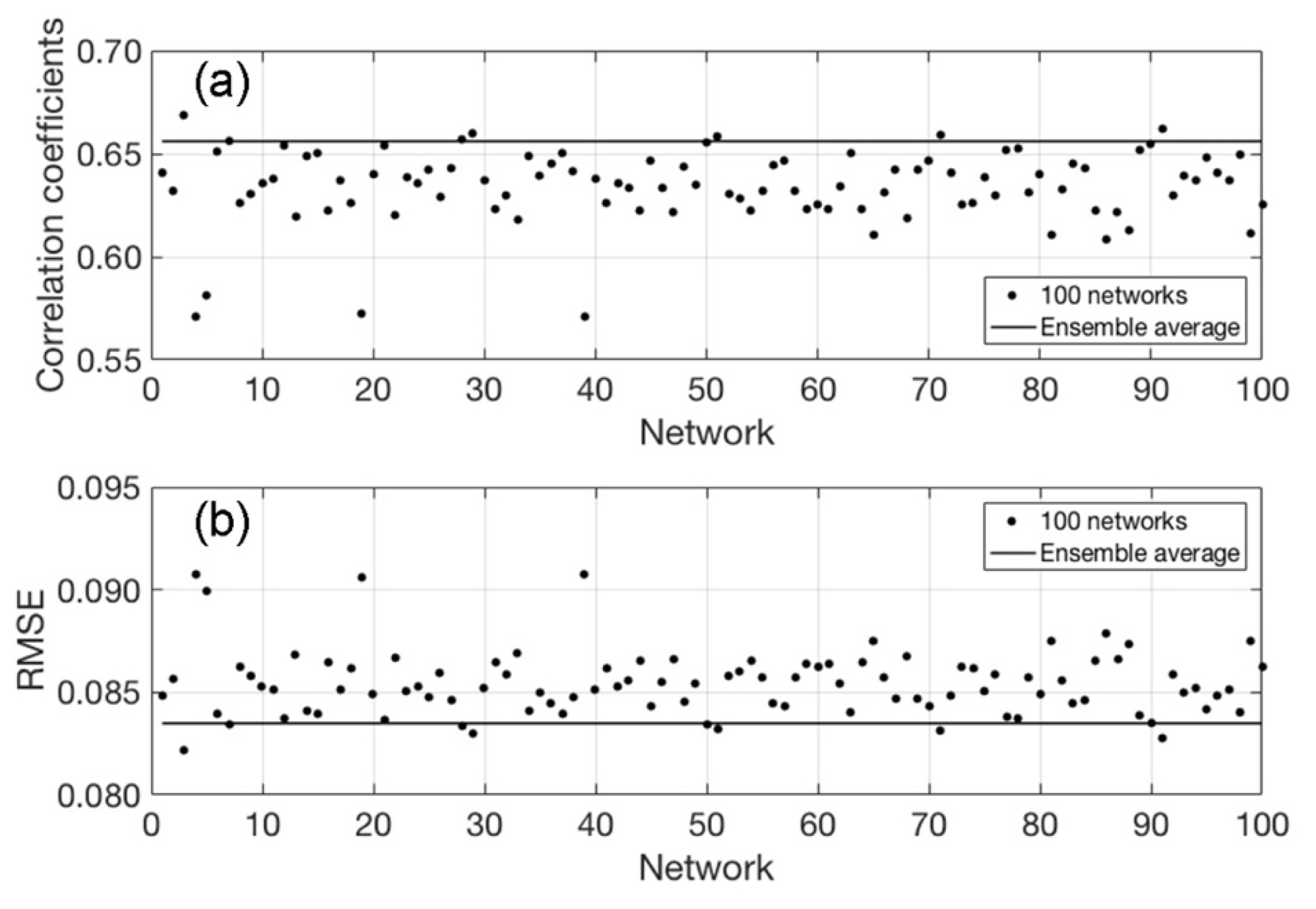
| R and RMSE | DNN_MPF (No SIC) | DNN_MPF +ObsSIC | DNN_MPF +AMSRSIC | DNN_MPF +NASASIC |
|---|---|---|---|---|
| Training R | 0.67 ± 0.02 | 0.66 ± 0.02 | 0.65 ± 0.03 | 0.65 ± 0.02 |
| Validation R | 0.61 ± 0.03 | 0.63 ± 0.03 | 0.60 ± 0.03 | 0.61 ± 0.03 |
| Test R | 0.60 ± 0.03 | 0.63 ± 0.03 | 0.60 ± 0.03 | 0.61 ± 0.03 |
| Total R | 0.65 ± 0.02 | 0.65 ± 0.02 | 0.64 ± 0.02 | 0.65 ± 0.02 |
| Training RMSE | 0.083 ± 0.002 | 0.082 ± 0.002 | 0.084 ± 0.002 | 0.085 ± 0.002 |
| Validation RMSE | 0.088 ± 0.004 | 0.083 ± 0.003 | 0.089 ± 0.003 | 0.088 ± 0.004 |
| Test RMSE | 0.089 ± 0.003 | 0.084 ± 0.004 | 0.089 ± 0.004 | 0.089 ± 0.003 |
| Total RMSE | 0.084 ± 0.002 | 0.083 ± 0.002 | 0.085 ± 0.002 | 0.086 ± 0.002 |
| Year | MPF > NASA Team SIC (SIC > 30%) | ||||
|---|---|---|---|---|---|
| DNN_MPF (No SIC) | DNN_MPF+ ObsSIC | DNN_MPF+ AMSRSIC | DNN_MPF+ NASASIC | Total Grid Cells | |
| 2000 | 0.09 | 0.08 | 0.27 | 0.17 | 49,127 |
| 2001 | 0.12 | 0.03 | 0.22 | 0.13 | 45,253 |
| 2002 | 0.13 | 0.04 | 0.21 | 0.10 | 47,358 |
| 2003 | 0.12 | 0.07 | 0.18 | 0.13 | 48,097 |
| 2004 | 0.10 | 0.04 | 0.20 | 0.12 | 47,545 |
| 2005 | 0.14 | 0.06 | 0.22 | 0.12 | 45,805 |
| 2006 | 0.14 | 0.06 | 0.25 | 0.12 | 45,281 |
| 2007 | 0.08 | 0.05 | 0.20 | 0.11 | 42,082 |
| 2008 | 0.09 | 0.09 | 0.16 | 0.11 | 43,445 |
| 2009 | 0.08 | 0.09 | 0.22 | 0.13 | 44,937 |
| 2010 | 0.09 | 0.04 | 0.22 | 0.12 | 42,775 |
| 2011 | 0.07 | 0.05 | 0.19 | 0.10 | 41,503 |
| 2012 | 0.09 | 0.03 | 0.11 | 0.09 | 39,476 |
| 2013 | 0.06 | 0.02 | 0.13 | 0.08 | 43,269 |
| 2014 | 0.07 | 0.05 | 0.17 | 0.09 | 43,127 |
| 2015 | 0.03 | 0.01 | 0.11 | 0.07 | 41,843 |
| 2016 | 0.09 | 0.02 | 0.16 | 0.08 | 40,403 |
| 2017 | 0.04 | 0.05 | 0.11 | 0.08 | 41,081 |
| 2018 | 0.06 | 0.05 | 0.10 | 0.08 | 40,231 |
| 2019 | 0.04 | 0.03 | 0.09 | 0.07 | 39,867 |
| Average | 0.09 | 0.05 | 0.18 | 0.11 | 43,625 |
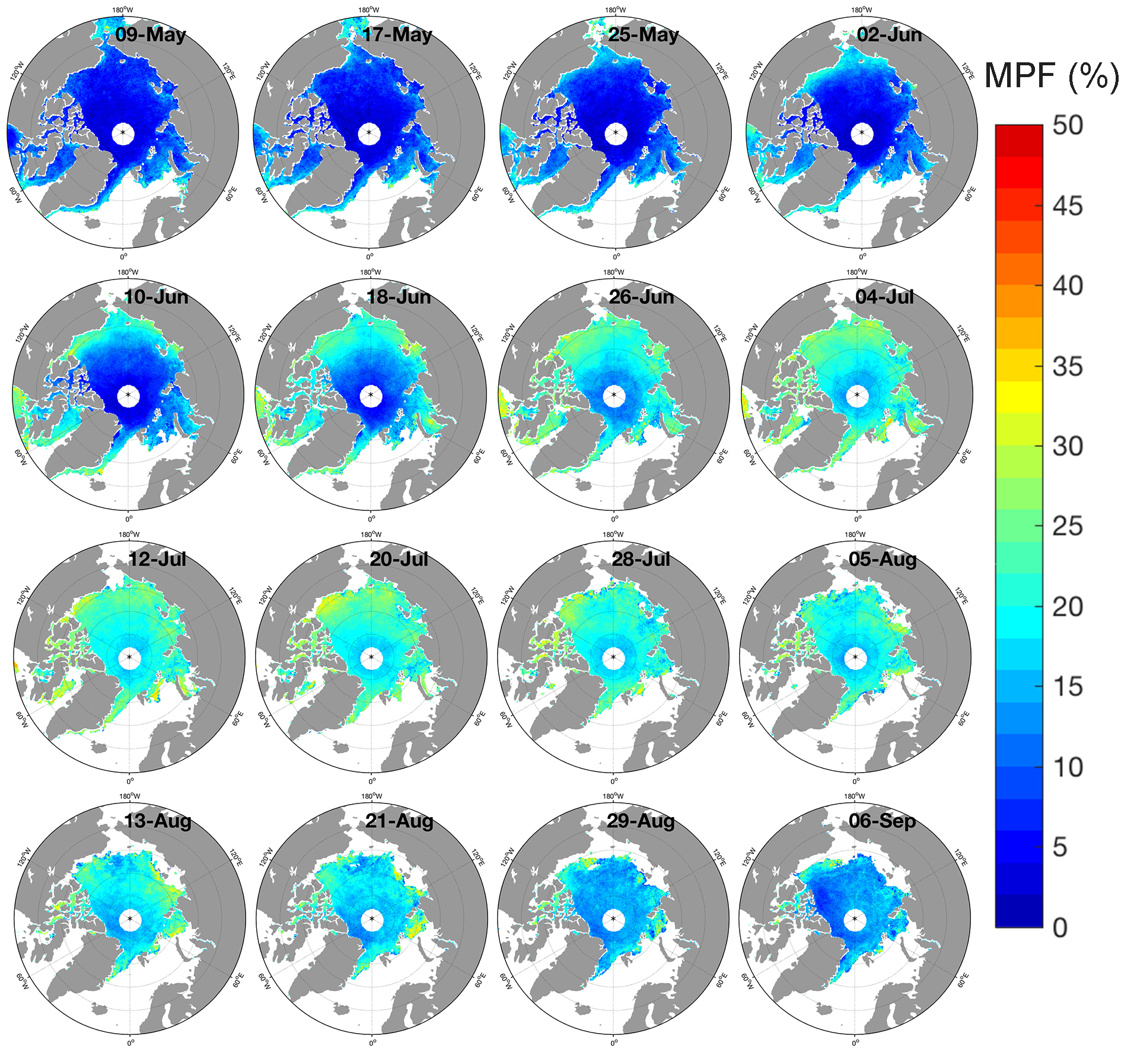
| Date | DNN_MPF | DNN_SIC |
|---|---|---|
| 05/09 | 2.61 | 5.96 |
| 05/17 | 2.45 | 5.83 |
| 05/25 | 2.27 | 5.49 |
| 06/02 | 2.00 | 4.76 |
| 06/10 | 1.87 | 3.99 |
| 06/18 | 1.77 | 3.54 |
| 06/26 | 1.63 | 3.09 |
| 07/04 | 1.45 | 2.67 |
| 07/12 | 1.37 | 2.56 |
| 07/20 | 1.39 | 2.61 |
| 07/28 | 1.47 | 2.82 |
| 08/05 | 1.57 | 3.11 |
| 08/13 | 1.71 | 3.39 |
| 08/21 | 1.81 | 3.63 |
| 08/29 | 2.00 | 4.05 |
| 09/06 | 2.23 | 4.43 |
| Average | 1.85 | 3.87 |
| Groups | R | RMSE (%) | Mean (%) | Standard Deviation (%) |
|---|---|---|---|---|
| 1 | −0.0080 | 15.63 | 18.11 | 10.97 |
| 2 | −0.0295 | 15.80 | 18.09 | 10.97 |
| 3 | −0.0096 | 15.63 | 18.06 | 10.94 |
| 4 | 0.0067 | 15.74 | 18.04 | 11.28 |
| 5 | 0.0049 | 15.56 | 18.10 | 11.01 |
| 6 | −0.0159 | 15.71 | 18.12 | 10.99 |
| 7 | 0.0035 | 15.44 | 17.99 | 10.83 |
| 8 | 0.0155 | 15.56 | 18.12 | 11.13 |
| 9 | 0.0028 | 15.62 | 18.02 | 11.07 |
| 10 | 0.0028 | 15.61 | 18.16 | 11.06 |
| Year | May 09 | May 17 | ||||||
|---|---|---|---|---|---|---|---|---|
| DNN_MPF | DNN_MPF_ClearSky | UH_MPFv2 | UB_MPF | DNN_MPF | DNN_MPF_ClearSky | UH_MPFv2 | UB_MPF | |
| 2003 | 7.65 | 5.70 | 5.26 | 9.00 | 9.07 | 7.00 | 7.83 | 9.68 |
| 2004 | 8.04 | 4.81 | 5.26 | 8.98 | 7.75 | 5.50 | 5.94 | 10.30 |
| 2005 | 7.82 | 6.16 | 7.59 | 10.00 | 8.30 | 7.07 | 7.06 | 10.00 |
| 2006 | 8.50 | 6.94 | 9.55 | 9.70 | 8.72 | 7.75 | 10.36 | 9.94 |
| 2007 | 8.10 | 6.20 | 9.82 | 9.95 | 7.33 | 6.80 | 8.83 | 10.89 |
| 2008 | 7.61 | 6.10 | 9.06 | 7.60 | 8.06 | 6.60 | 8.15 | 8.69 |
| 2009 | 6.83 | 5.46 | 10.74 | 10.10 | 8.22 | 7.39 | 10.71 | 10.78 |
| 2010 | 7.31 | 6.60 | 7.95 | 10.36 | 7.87 | 7.18 | 8.21 | 10.63 |
| 2011 | 6.84 | 5.73 | 9.40 | 9.15 | 7.81 | 7.34 | 8.89 | 9.51 |
| Average | 7.63 | 5.97 | 8.29 | 9.43 | 8.12 | 6.96 | 8.44 | 10.05 |
© 2020 by the authors. Licensee MDPI, Basel, Switzerland. This article is an open access article distributed under the terms and conditions of the Creative Commons Attribution (CC BY) license (http://creativecommons.org/licenses/by/4.0/).
Share and Cite
Ding, Y.; Cheng, X.; Liu, J.; Hui, F.; Wang, Z.; Chen, S. Retrieval of Melt Pond Fraction over Arctic Sea Ice during 2000–2019 Using an Ensemble-Based Deep Neural Network. Remote Sens. 2020, 12, 2746. https://doi.org/10.3390/rs12172746
Ding Y, Cheng X, Liu J, Hui F, Wang Z, Chen S. Retrieval of Melt Pond Fraction over Arctic Sea Ice during 2000–2019 Using an Ensemble-Based Deep Neural Network. Remote Sensing. 2020; 12(17):2746. https://doi.org/10.3390/rs12172746
Chicago/Turabian StyleDing, Yifan, Xiao Cheng, Jiping Liu, Fengming Hui, Zhenzhan Wang, and Shengzhe Chen. 2020. "Retrieval of Melt Pond Fraction over Arctic Sea Ice during 2000–2019 Using an Ensemble-Based Deep Neural Network" Remote Sensing 12, no. 17: 2746. https://doi.org/10.3390/rs12172746