Article

Open-Surface River Extraction Based on Sentinel-2 MSI Imagery and DEM Data: Case Study of the Upper Yellow River

1
State Key Laboratory of Hydroscience and Engineering, Tsinghua University, Beijing 100084, China
2
Key Laboratory of Digital Earth Science, Institute of Remote Sensing and Digital Earth, Chinese Academy of Sciences, Beijing 100094, China
3
Key Laboratory of River Regulation and Flood Control of the Ministry of Water Resources, Changjiang River Scientific Research Institute, Wuhan 430010, China
*
Author to whom correspondence should be addressed.
Remote Sens. 2020, 12(17), 2737; https://doi.org/10.3390/rs12172737
Submission received: 10 July 2020 / Revised: 20 August 2020 / Accepted: 21 August 2020 / Published: 24 August 2020

Abstract

:
Water is essential for the survival of plants, animals, and human beings. It is imperative to effectively manage and protect aquatic resources to sustain life on Earth. Small tributaries are an important water resource originating in mountain areas, they play an important role in river network evolution and water transmission and distribution. Snow and cloud cover cast shadows leading to misclassification in optical remote sensing images, especially in high-mountain regions. In this study, we effectively extract small and open-surface river information in the Upper Yellow River by fusing Sentinel-2 with 10 m resolution optical imagery corresponding to average discharge of the summer flood season and the 90 m digital elevation model (DEM) data. To effectively minimize the impact of the underlying surface, the study area was divided into five sub-regions according to underlying surface, terrain, and altitude features. We minimize the effects of cloud, snow, and shadow cover on the extracted river surface via a modified normalized difference water index (MNDWI), revised normalized difference water index (RNDWI), automated water extraction index (AWEI), and Otsu threshold method. Water index calculations and water element extractions are operated on the Google Earth Engine (GEE) platform. The river network vectors derived from the DEM data are used as constraints to minimize background noise in the extraction results. The accuracy of extracted river widths is assessed using different statistical indicators such as the R-square (R2) value, root mean square error (RMSE), mean bias error (MBE). The results show the integrity of the extracted small river surface by the RNDWI index is optimal. Overall, the statistical evaluation indicates the accuracy of the extracted river widths is satisfactory. The effective river width that can be accurately extracted based on satellite images is three times the image resolution. Sentinel-2 MSI images with a spatial resolution of 10 m are used to find that the rivers over 30 m wide can be connectedly, accurately extracted with the proposed method. Results of this work can enrich the river width database in the northeast Tibetan Plateau and its boundary region. The river width information may provide a foundation for studying the spatiotemporal changes in channel geometry of river systems in high-mountain regions. They can also supplement the necessary characteristic river widths information for the river network in unmanned mountain areas, which is of great significance for the accurate simulation of the runoff process in the hydrological model.

Graphical Abstract

1. Introduction

River systems across the globe develop from source regions, stretch over the land, and finally flow into the sea as the “blood vessels of the earth”. They gather, transmit, and distribute water, sediment, and biogenic substances in the basin thus closely linking together multi-temporal scale processes such as hydrological cycles, landform changes, and ecological evolution. Water bodies interact with the atmosphere, vegetation, environment, and geomorphology to play an important role in regional economic and environmental sustainability, drinking water safety, and ecological security [1,2,3,4,5]. Spatial characteristics such as river width, water surface area, river channel form, and braiding index are essential for discharge estimation [6,7], flood forecasting [8,9], climate change research [10,11,12], hydro-geomorphological process assessment [13,14], and landscape evolution analysis [15].
In recent years, rapid advancements in satellite remote sensing, computer image processing, and artificial intelligence (AI) technologies, as well as the abundance of basic geographic information data such as digital elevation models (DEMs), has allowed for remarkable progress in river network system research [16,17,18,19,20]. Satellite-based imagery allows for accurate water body detection, extraction, and classification as it encompasses both spatial and spectral characteristics. Extracted water area, geometric shape, water quality status, and ecological environment information has been applied in the investigation and macro-monitoring of water resources as well as environmental protection, natural disaster forecasting, and land classification applications [21,22,23,24,25,26]. Many researchers have successfully used the Google Earth Engine (GEE) platform for large-scale water extraction and change detection [10,27,28,29]. The GEE cloud platform integrates many open source remote sensing images and various derivative products, providing strong support for efficient water body extraction.
Different water indices have been constructed using the spatial and spectral characteristics of remote sensing images to accurately extract water body information. The most commonly used index is the normalized difference water index (NDWI) proposed by Mcfeeters based on the normalized difference vegetation index (NDVI) concept [30]. Many other indices have been developed according to different background information. Ouma et al. [31] for example, constructed the NDWI3 model using near-infrared and mid-infrared bands for edge detection of actual shorelines (real land-water interfaces) by considering the effects of suspended solid particles, lake edge depth, and water body mobility. Taking advantage of surface reflectance, Fisher et al. [32] created the WI2015 index through linear discriminant analysis to determine the classification coefficient of an optimal segmentation training area with high classification accuracy.
Classification algorithms proposed in the past based on remote sensing images are mostly dependent on existing reference data or known input data as training samples [17,18,25,26,33]. The influence of high altitudes, narrow channels, complex topographies, and long-term cloud cover, however, make it very difficult to extract rivers in unmanned regions of the Tibetan Plateau. As the birthplace of many large rivers, such as the Yangtze River, the Yellow River, the Yarlung Zangbo River, and the Lantsang River, the Tibetan Plateau is typical of a region lacking hydrological data: Its ecological environment is fragile and sensitive to external disturbances caused by climate change and anthropogenic activity. Global water products such as global river widths from Landsat (GRWL) by Allen and Pavelsky [10] and global surface water by Pekel et al. [12] have performed well on Tibetan Plateau. GRWL products allow for precise data extraction of rivers with widths over 90 m and Pekel et al.’s products perform well in terms of spatiotemporal changes in rivers. However, both products yield incomplete characterizations of small rivers (<90 m width), and there has been no detailed study within a specific time range in the Tibetan Plateau region.
River discharge plays a vital role in the hydrological cycle. Kebede et al. [34] used the effective widths from Landsat images to estimate discharges of the Lhasa River via fundamental flow equations/models. Effective river widths are highly correlated with river discharge data, discharge simulation can be fulfilled in hydrological models based on these characteristic river widths. Tributaries connected to the main streams, though with relatively small size, are also important water resources to the Upper Yellow River Basin. Their accurate extraction plays an important role in discharge retrieval and runoff simulation of the hydrological model in the source area of the river. Based on characteristic discharge, characteristic river widths and corresponding hydraulic variables, geomorphological researches including river network distribution and development can be performed. Small rivers/tributaries are abundant in small water catchments and unmanned zones of the high-mountain regions of the Tibetan Plateau. However, there are extremely few hydrological stations there, making it nearly impossible to obtain in situ data. There is an urgent need to improve the extraction accuracy of river surface data, especially for small rivers (width < 90 m). High-resolution remote sensing technology may fill this gap to yield accurate small-river channel width extraction to serve hydrological models and various geomorphological researches in this and other high-mountain regions.
The Upper Yellow River is the main water source area of the entire Yellow River. The area above Anningdu hydrological station (see Figure 1) is of particular concern, as its runoff generation accounts for 60% of the total runoff of the entire basin. Therefore, the Upper Yellow River was taken as the observation area in this study. Sentinel-2 with 10 m spatial resolution multispectral instrument (MSI) remote sensing images during the 2017 flood season were used to extract river surface. Images within the date range of in situ hydrological station daily-discharge between 1–2 times average discharge of the summer flood season from 2007 to 2017 were selected. We fused the SRTM 90 m DEM data and 10 m resolution Sentinel-2 images to enhance the small-river extraction accuracy. We chose three water body indices, including the modified normalized difference water index (MNDWI), the revised normalized difference water index (RNDWI), and the automated water extraction index (AWEI), to determine the optimal extraction results. The accuracy of extracted river positions and river widths was evaluated with GRWL and hydrological station in situ data. The “water bodies” referred to below are rivers unless otherwise stated.

2. Study Area and Data
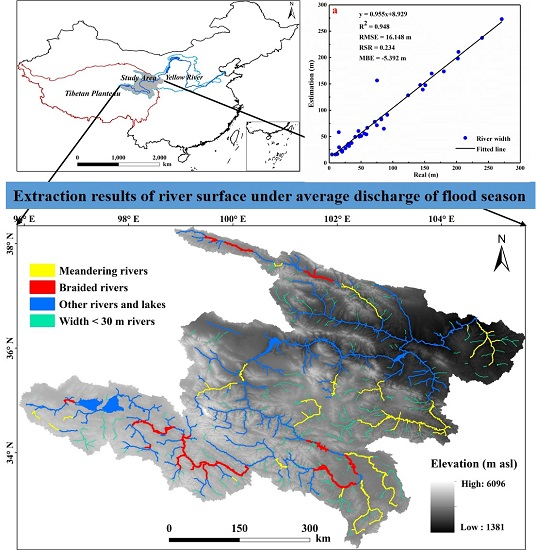
2.1. Study Area

The study area is located in the Upper Yellow River in the northeast part of the Tibetan Plateau, bordering Qinghai, Sichuan, and Gansu provinces. It covers a total area of about 250,944.65 km2 (Figure 1). This area consists of a series of alternating mountains, valleys, and hills with an elevation range of 1390–6252 m. It has a typical plateau continental climate, alternating between hot and cold seasons and wet and dry seasons. There is relatively little annual temperature difference and large daily temperature difference, with lengthy sunshine time and strong solar radiation throughout. Water supply mainly comes from melting mountain snow and ice. There is more rainfall in summer and less rainfall in winter.
The flood season of 2017 (16 June to 31 October) was selected as the study period according to the regional hydrological conditions. The “summer flood season” in the study area was defined according to a previous article by Bing et al. [35].

2.2. Data

2.2.1. Sentinel-2 MSI Imagery

The Sentinel-2 satellite images used in this study were collected from 16 June to 31 October 2017, on the GEE cloud platform. Sentinel-2 is a European wide-swath, high-resolution, and multi-spectral imaging mission developed by the European Space Agency (ESA) [36]. It provides continuous services relying on multi-spectral high-resolution optical observations over global terrestrial surfaces. The key mission objectives for Sentinel-2 are to provide systematic global acquisitions of high-resolution multi-spectral imagery (MSI) with a high revisit frequency (10 days for one satellite, 5 days for two satellites) and observations for the next generation of operational products (e.g., land-cover maps, land change detection maps [37]). Sentinel-2 MSI samples 13 spectral bands spanning from the visible and the near infrared (VNIR) to the short wave infrared (SWIR), with four bands at 10 m, six at 20 m, and three at 60 m spatial resolution [38]. Table 1 provides more detailed information from the Sentinel-2 User Handbook. The Sentinel-2 satellite provides level-1C (L1C) and level-2A (L2A) products; we used the top-of-atmosphere products (L1C data) in this study.
The composition of different underlying surfaces affects the integrity of river surface extractions in the study area. We selected Band 2 (Blue), Band 3 (Green), Band 4 (Red), Band 8 (NIR), Band 11 (SWIR), and Band 12 (SWIR) to support our work. Band 11 and Band 12 were resampled to 10 m to ensure the uniform resolution of the water indices.

2.2.2. River Network from DEM

Drainage network extraction plays an important role in geomorphologic analyses and hydrologic modeling, among other applications. Flow enforcement is conducted by overlaying information of known river maps to DEMs for improved drainage network extraction [20]. Wu et al. [20] and Bai et al. [39] used an enhanced flow enforcement method without elevation modification towards an accurate and efficient drainage network extraction. In addition to preserving the Boolean-value information as to whether a DEM pixel belongs to a stream, the proposed method can accurately preserve and facilitate the use of topological relations among mapped streamlines and the morphological information of each mapped streamline.
We used the Drainage Network Extraction Tool (DNET) developed by Wu et al. and Bai et al. [20,39] to extract river networks from the SRTM 90 m DEM; this DNET adopts the Horton–Strahler classification method [40,41]. SRTM 90 m DEM data was downloaded from “http://www.gscloud.cn/”. We used topographic maps and other auxiliary data to manually edit the DEMs to remove influence of buildings and other extraneous surface features. We set the minimum confluence area to 7.29 km2 after trial-and-error revealed this was appropriate. We extracted a total of seven orders of river networks according to this minimum area using the DNET. The rivers of orders 3–7 are shown in Figure 1. We measured river widths of different orders artificially on Google Earth, then established buffer zones of the river networks based on the measured widths to de-noise the river surface extraction results.

2.2.3. Hydrological Station Data

We collected data from 39 hydrological stations in the study area during the summer flood seasons from 2007 to 2017 from the Hydrology Yearbook of Yellow River [42]. More than 80% of these stations were located in the eastern and northern regions, as shown in Figure 1. For detailed information of hydrological stations in each sub-region, please see Table 2.

3. Methods

The upstream part of the river is narrower than the downstream and its tributaries are narrower than the main stream. The river widths of many tributaries are 2–3 pixels in the Sentinel-2 MSI image. Some tributaries are smaller than one pixel; their images appear as mixed pixels and their spectral information is weaker than the background. We comprehensively considered the topographic and geomorphological characteristics of the study area, its climatic conditions, the spatial distribution characteristics of the rivers, the band characteristics of Sentinel-2 data, and the spectral characteristics of the river on remote sensing images to extract the river surface as accurately as possible.
Misleading information caused by topographic shadows, cloud shadows, and snow cover make it difficult to distinguish the water body from other surfaces. Considering the effect of these factors and the interference of the environmental background, we deployed a three-step process to extract the water body. First, we obtained five sub-regions by merging the catchments of each hydrological station according to the differences in underlying surface, elevation, and river level. Next, we adopted three water body indices for input to Otsu’s threshold segmentation method for automatic water surface extraction. Finally, we built a buffer zone along the river system using the drainage network data to constrain the range of river surface extraction and minimize background noise. The data processing work mainly included discharge determination, the selection of Sentinel-2 images, study area subdivision, and calculation of water body indices on the GEE cloud platform. De-noising, vector data editing, and connectivity of the rivers were conducted in ArcGIS 10.2. The flow chart of the research is shown in Figure 2.

3.1. Data Pre-Processing

3.1.1. Study Area Subdivision

The study area was subdivided into five sub-regions as per the composition of the underlying surface and elevation information from the DEMs (Figure 1). First of all, we took 39 hydrological stations and their catchment boundaries as the most important division standard, combined with the information of DEM elevation and land use/cover change of China in 2015 (LUCC2015) [43]. The elevation and land cover types in small catchments divided by hydrological stations were statistically analyzed. Then, the adjacent small catchments with similar land cover types and elevation difference were combined to generate five larger sub-regions (see A–E in Figure 1). The elevation difference of study area is greatest between the eastern and western parts, and the types of land cover differ throughout. Sub-region A is dominated by sandy lands, Sub-region B is dominated by sandy lands and grasslands, Sub-region C is dominated by forestlands and grasslands, Sub-region D is dominated by dry lands and urban lands, and Sub-region E is dominated by forestlands, rural settlements and marsh lands. Sub-regions A and B were more affected by clouds and snow than sub-regions C, D, or E. Table 2 gives detailed information for the five sub-regions.

3.1.2. Discharge Calculation and Image Selection

We collected data from 40 hydrological stations in the study area during the summer flood seasons from 2007 to 2017 from the Hydrology Yearbook of Yellow River [42]. This set of data contains coordinate position, date, velocity, measured discharge, and river width, among other information. Generally, the bankfull discharge and corresponding parameters (e.g., river width, water depth) have important physical significance to geomorphological evolution of river systems and hydrological modelling. However, the bankfull discharge recurrence period is longer than the average discharge period of the flood season. Van den Berg [44] used average flood season discharge rather than bankfull discharge to conduct similar research, which is widely accepted in researches and applications. Therefore, the average discharge (AD) of the summer flood season over 39 hydrological stations in 11 years was calculated here—only one station which is located in a seasonal stream was removed from our data set.
The images of each catchment in the summer flood season of 2017 were determined from the GEE to determine the date when a single one-day image could completely cover the basin. We then established a one-to-one correspondence between the acquisition date of remote sensing images and the measured discharge of 39 hydrological stations in 2017. We selected the full-coverage images closest to the average discharge day to extract rivers, ensuring their widths were closest to the actual river widths under the average discharge condition. For the hydrological stations distributed in sub-regions C, D, and E, we only selected the images of the day closest to the average discharge. Images of sub-regions A and B were heavily affected by clouds and snow; we selected images of the first three dates closest to the average discharge to composite complete images to cover the sub-regions. The relationship between daily-discharge image and average discharge of the summer flood season is shown in Figure 3. The ratios of 29 stations were between 0.75 and 1.75.

3.1.3. Water Index Selection

Xu et al. [45] constructed the modified normalized differential water index (MNDWI) by analyzing spectral feature of buildings to enhance the contrast between water bodies and buildings in urban areas, thus extracting water body information easily and accurately. Feyisa et al. [46] introduced an automated water extraction index (AWEI) to improve the classification accuracy of regions including shadows and dark surfaces, which are likely when either topography is pronounced, background noise is prevalent, or both. In order to weaken the effect of mixed pixels, vegetation, and mountain shadows, Cao et al. [47] constructed a revised normalized differential water index (RNDWI) to extract water surfaces using the short-wave infrared band and red band. Given the effects of topographies, shadows, and clouds in the study area, we isolated a small high-altitude region and another low-altitude region from which to extract water bodies from images using the MNDWI, RNDWI, water index (WI2015), and AWEI. The application characteristics of each index can be found in reference [48]. For those areas covered by multi-date images, we used the maximum value of the water index to composite a raster result to improve the recognition accuracy of the water body boundary.
These tests on actual images revealed that MNDWI, RNDWI, and AWEI were well-suited to water body extraction in the Upper Yellow River. Six of the 13 Sentinel-2 data bands were used to construct MNDWI, RNDWI, and AWEI as follows:
M N D W I = ( ρ g r e e n ρ s w i r 1 ) ( ρ g r e e n + ρ s w i r 1 )
R N D W I = ( ρ s w i r 2 ρ r e d ) ( ρ s w i r 2 + ρ r e d )
A W E I = ρ b l u e + 2.5 × ρ g r e e n 1.5 × ( ρ n i r + ρ s w i r 1 ) 0.25 × ρ s w i r 2
where ρ is the apparent reflectance value of spectral bands of Sentinel-2, including blue (band 2), green (band 3), red (band 4), NIR (band 8), SWIR1 (band 11), and SWIR2 (band 12). The spatial resolution of all six bands was uniformly resampled to 10 m.

3.1.4. Water Body Extraction

Nobuyuki Otsu [49] built a benchmark algorithm in 1979 to identify optimal thresholds for initial segmentations; this method provides excellent binary results in case of noisy images. The Otsu threshold determined from a histogram curve was adopted here to create water and non-water binary-class maps. Otsu’s threshold is dependent on the ratio of water to non-water surfaces in index-based water body extractions [50]; this method did not yield satisfying results in this study. We instead used Otsu’s method to determine the initial base threshold, then adjusted the threshold several times and integrated visual interpretations to determine the optimal segmentation threshold. The visual interpretation criterion was designed to minimize background noise under the condition that water bodies were extracted completely. The MNDWI had better extraction results than other techniques in parts of the study area dominated by urban and sandy lands (Figure 4e). The AWEI had better results in parts dominated by vegetation (Figure 4d). The RNDWI significantly outperformed the other two indices in the extraction of small rivers (Figure 4f).
The study area is located in the Upper Yellow River, where the overall river widths are relatively narrow. The RNDWI index was adopted in all five sub-regions to extract these small rivers properly. The other two indices were selected as supplements according to the elevation and underlying surface of different sub-regions. In order to reduce noise and improve the accuracy and integrality of river extraction, we used the intersection results of RNDWI and MNDWI, RNDWI and AWEI in sub-regions A and D, sub-regions B and C for orders 5 to 7 river network from the SRTM 90 m DEM. We used the union results of RNDWI and MNDWI, RNDWI and AWEI in sub-regions A and D, and sub-regions B and C for orders 3 to 4 river network. Multiple tests and visual interpretations revealed that the thresholds of MNDWI in sub-regions A and D were 0.15 and 0.13, respectively. The thresholds of RNDWI in sub-regions A, B, C, D, and E were 0.14, 0.15, 0.22, 0.16, and 0.15, respectively. The thresholds of AWEI sub-regions in B and C were −2000 and −800, respectively (see Table 2). We transformed the images generated by the water indices into vector features in order to create shape files for de-noising in ArcGIS 10.2.

3.2. Data Post-Processing

3.2.1. De-Noising Based on DEM

There was an abundance of noise in the water bodies we extracted due to vegetation, snow, clouds, and mountain shadows. River networks extracted using DNET from the SRTM 90 m DEM were used as an aid to remove the majority of the noise by setting up a buffer zone alongside, as mentioned above. Considering the differences in river shapes and phases between the extracted drainage networks and Google Earth images, order 3 and 4 river networks were given a buffer width of 800 m. The order 5 river network in the E sub-region was given a buffer width of 1500 m as it contains many braided rivers. Order 6 river networks in the A and C sub-regions were given a buffer width of 3000 m. The buffer width of order 5 and 6 river networks in other sub-regions was 1000 m, and the buffer width of order 7 river networks was 1200 m. The buffered river networks were used to constrain the extraction results based on water indices to remove background noise from outside the buffer zone (Figure 4d–f).
We found that a substantial amount of noise persisted inside the buffer zones, especially in urban regions and regions affected by clouds and mountain shadows, which needed to be removed manually. We first isolated the connected rivers in the buffer zones, and judged the properties of points outside the connected rivers. If they were obviously disconnected river points, we manually removed other noise and retained the river points (purple part in Figure 4g,i). If the point was not a river, we considered it noise and remove it. There was still quite a bit of noise in the connected rivers we selected, so we manually edited and de-noised the vector data. All operations were performed in ArcGIS 10.2.

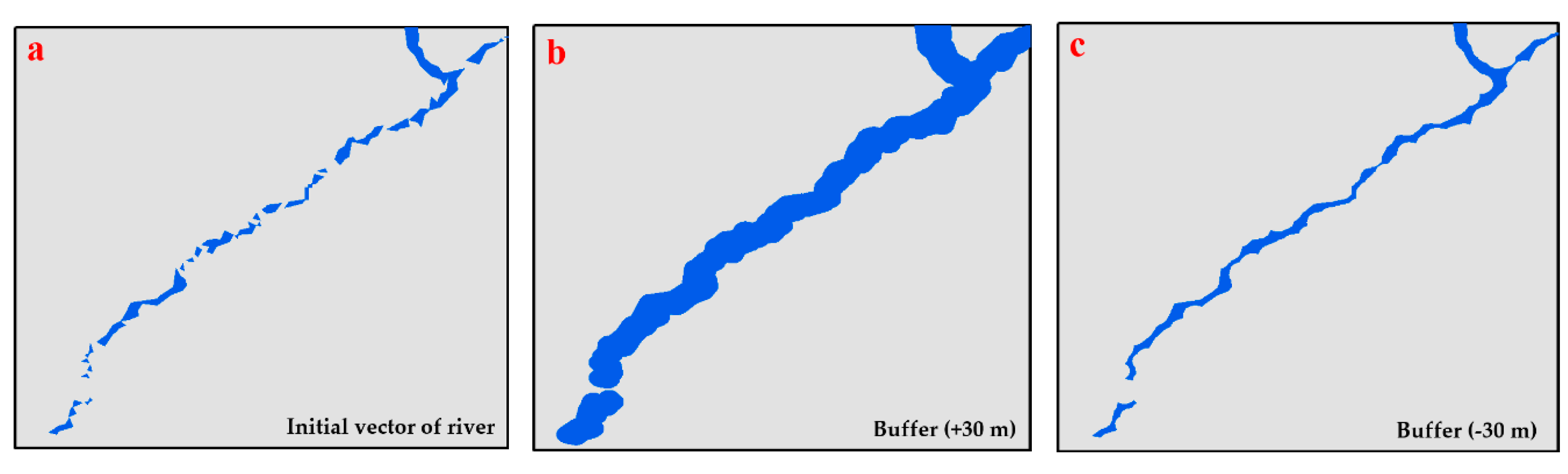
3.2.2. Connectivity Processing

Clouds, shadows, urban structures, bridges, and other factors created disconnection in the rivers we extracted. Some rivers were only between 1–3 pixels in a given image—some were even less than 1 pixel—thus making the extracted rivers disconnected. The disconnected rivers were generally less than 30 m by manual measurements. By buffering the extracted river feature, we tied to connect the disconnected rivers as much as possible for showing existence and a better present of a whole river network (Figure 5). Larger disconnected rivers were connected according to the river networks defined over the whole study area.

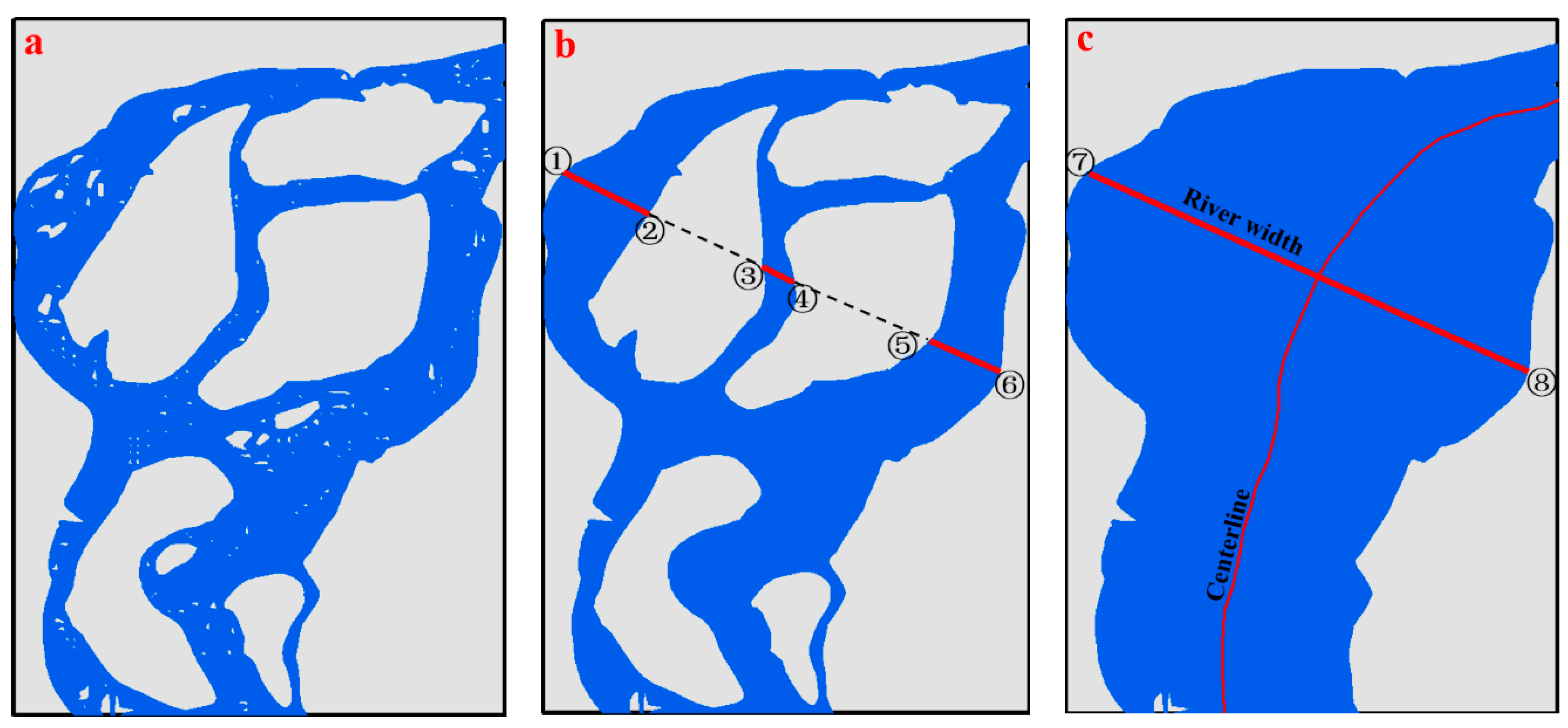
3.2.3. Map Generalization

Compared with the MNDWI and AWEI, the RNDWI extracted more details of small rivers in the study area; however, it produced more pepper and salt noise on the large rivers. Fusing the results of RNDWI and MNDWI, or RNDWI and AWEI and filling in the small gaps in the rivers to improve the beauty of extraction results. Actual shoals in a given river may have been partially or completely filled in this process (Figure 6). Two kinds of river width were defined: flow width and boundary width. The flow width refers to the width after removing the no flow water body, the red solid lines at Figure 6b. The boundary width is the farthest distance between the two sides of a river, corresponding to the red solid line in Figure 6c.

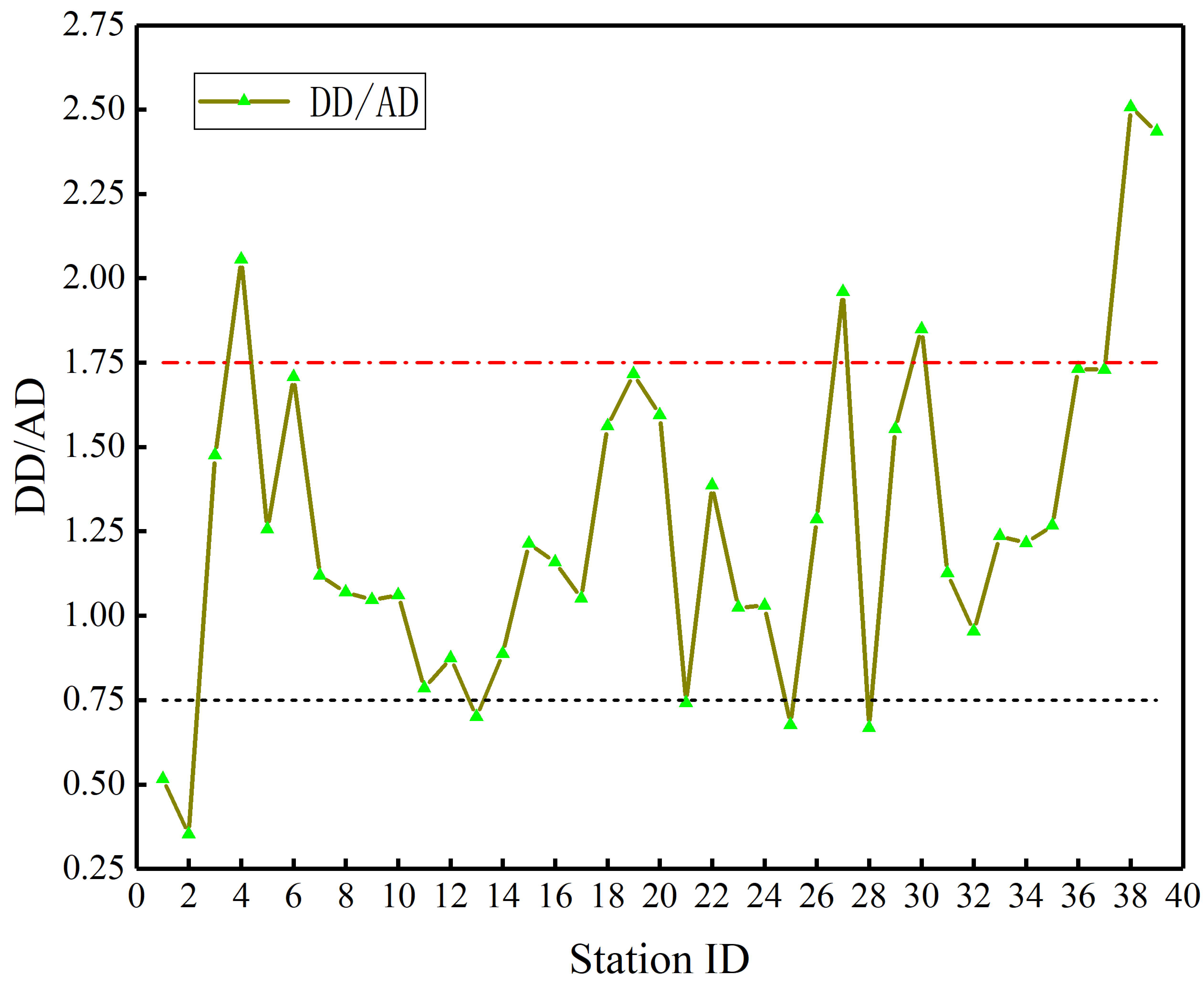
3.3. Accuracy Assessment

We evaluated the accuracy of the river surface extraction results according to (1) the qualitative river integrality and location accuracy and (2) the quantitative river width. The qualitative evaluation was performed by superposition analysis with GRWL from Allen and Pavelsky [10]. The linear regression accuracy of river widths was evaluated using in situ river widths from the 39 hydrological stations in date of images. Based on the literature [51,52,53,54,55,56,57], the linear regression model was evaluated using statistical indicators (R-Square (R2) [54], root mean square error (RMSE) [55,56], and mean bias error (MBE) [57]). Table 3 provides a classification of the performance that were used for the linear regression model evaluation.

4. Results

4.1. Spatial Distribution of Water Bodies

Figure 7 shows the spatial distribution of water bodies in the Upper Yellow River. By comparing the extraction results of the connected rivers (Figure 7, width > 30 m rivers) based on Sentinel-2 images with GRWL centerline products from Allen and Pavelsky [10], and comparing the extraction results of the connected rivers with river networks from the SRTM 90 m DEM data (Figure 8, ≥Order 4 rivers), we evaluated the spatial distribution of rivers and the detailed degree of river extraction in this area. Figure 7 shows that the river extraction results based on 10 m Sentinel-2 images were richer than the GRWL results from 30 m Landsat data, particularly for order 4–5 rivers. Figure 8 shows that the extraction results covered almost all order 5–7 rivers and most of the order 4 rivers. The spatial consistency is better for high-order rivers. This is in line with our focus on extracting smaller water bodies in the Upper Yellow River.

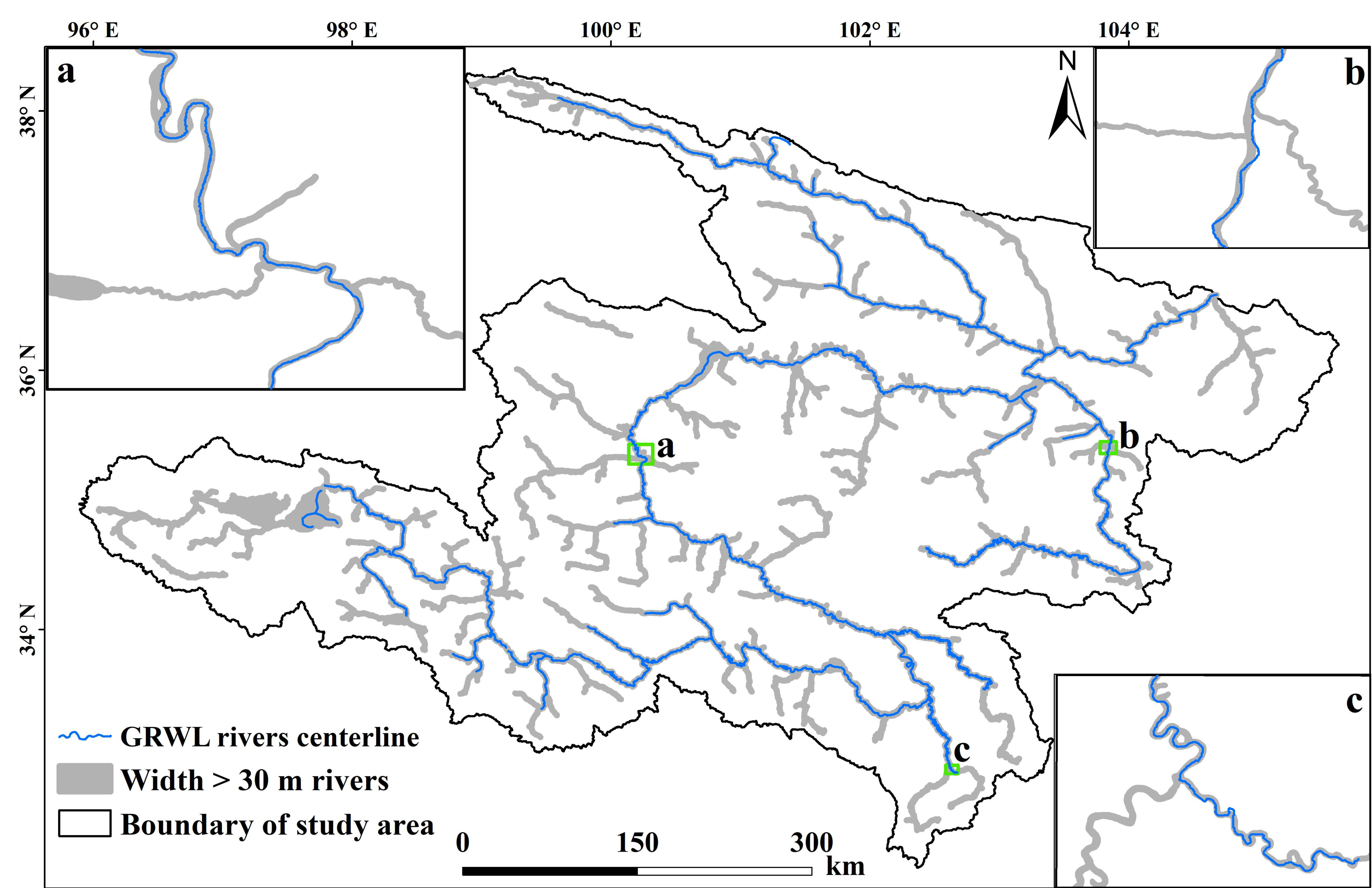
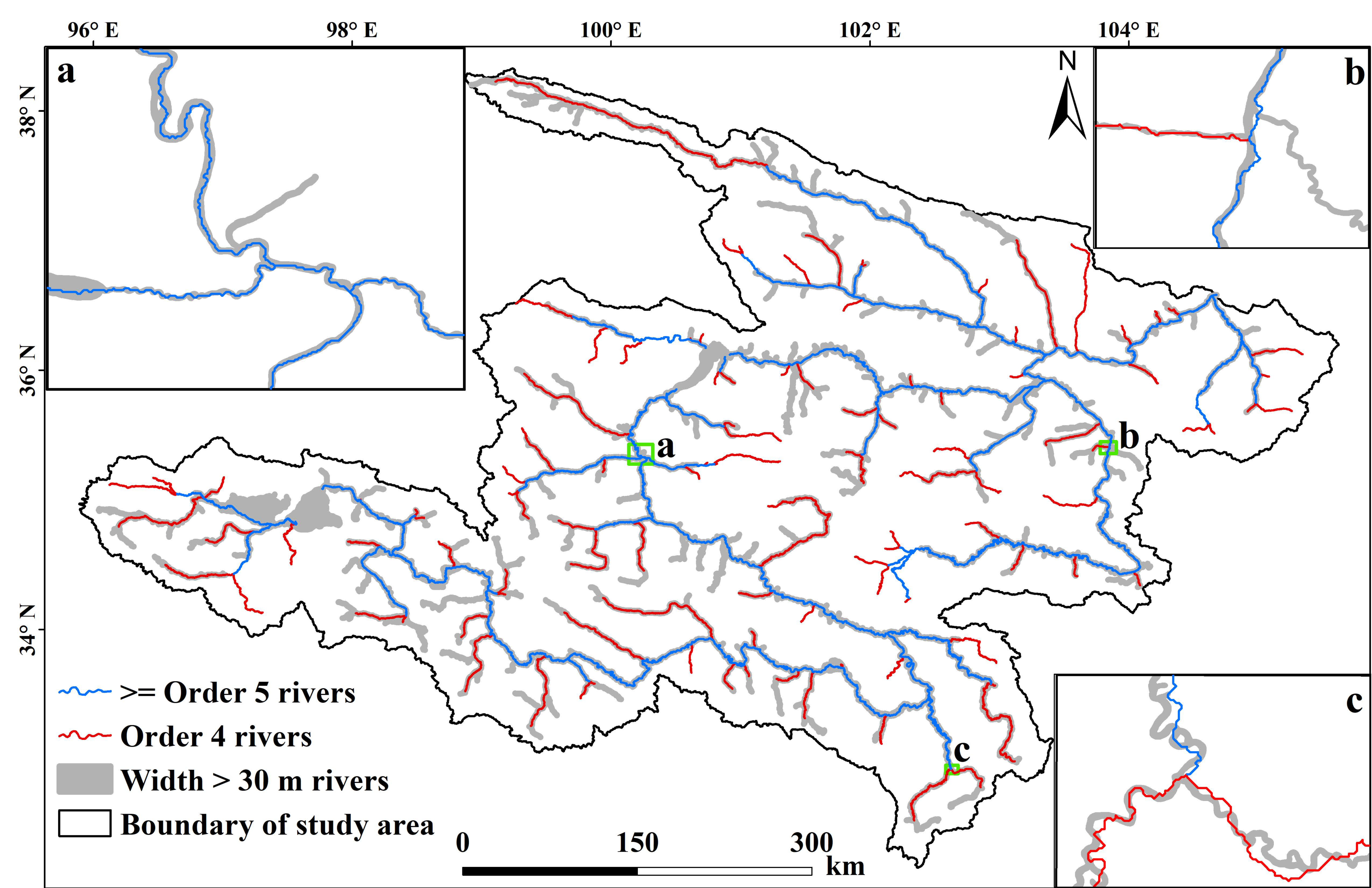
4.2. River Extraction Results from Sentinel-2

The extracted water bodies in the Upper Yellow River include connected rivers at least 30 m wide, partial disconnected rivers less than 30 m wide, two large lakes, and two large reservoirs that are connected to the river network (Figure 9). The extracted river orders are from 3 to 7 according to the river networks in the DNET. Based on the definitions of braided rivers and meandering rivers provided in the book entitled “Key Concepts in Geomorphology” [58], we collected remote sensing images in the low water stage and determined three river patterns (braided rivers, meandering rivers and other rivers) through calculation and visual interpretation. The locations of braided rivers, meandering rivers and other rivers are marked with different colors based on the extraction results in Figure 9. We chose cross-sections of different river patterns from the DEM to provide a comprehensive illustration. We found that meandering rivers belonged to confined rivers with stable bedrock controls on both sides; braided rivers were mostly unconfined and without bedrock controls, so their plane shapes were very unstable and changed significantly with time. Most of the other rivers had relatively strong bedrock controls. Some fell between braided and meandering rivers.

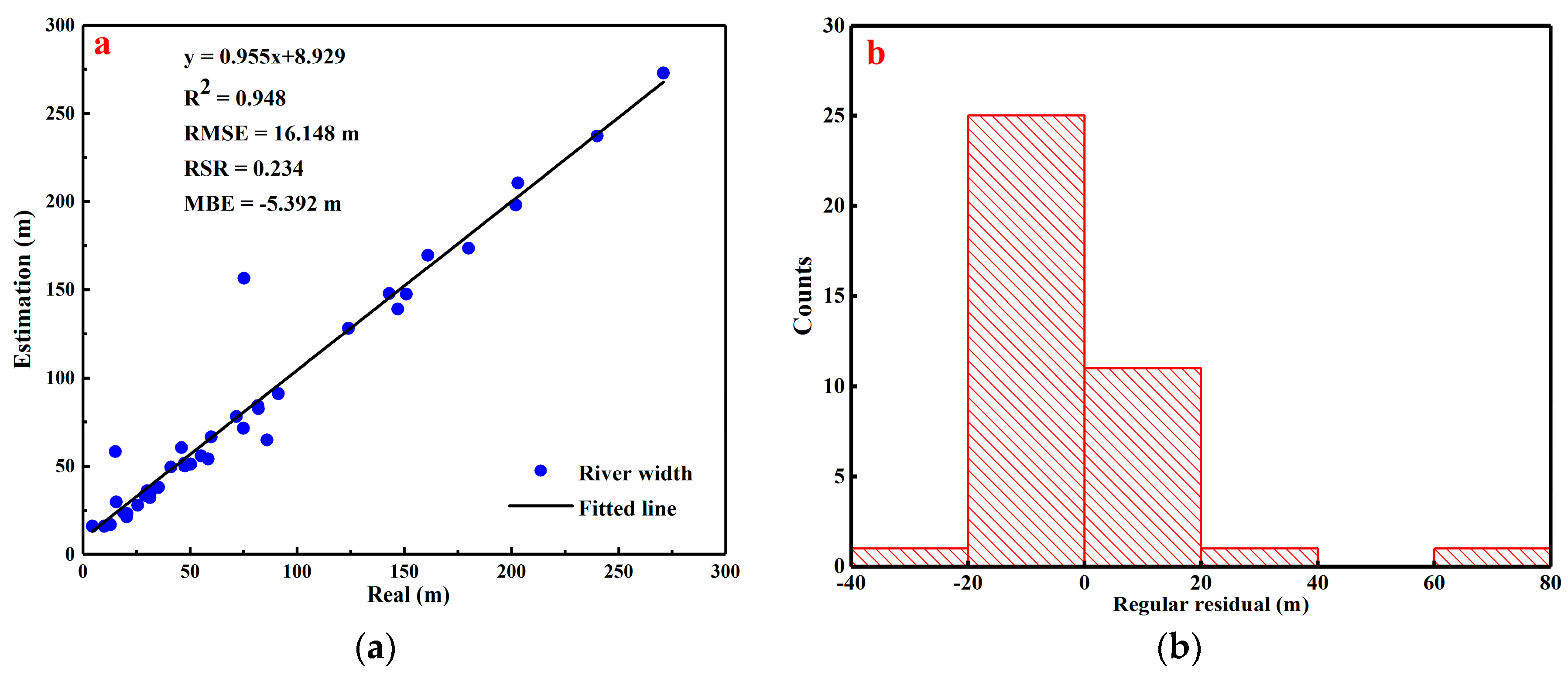
4.3. River Width Estimation

We determined the in situ river widths from 39 hydrological stations in the corresponding dates from the hydrological yearbook to verify the river width estimations extracted from Sentinel-2 satellite images. We first extracted the centerline of river and measured its orthogonal length, then took the distance between two intersection points as the river width. We measured the river widths three times with 5 m as the step length; the average value is given here as the final river width estimation. The statistical evaluation showed a satisfactory result, the R2, RSR, RMSE, and MBE of the estimated river widths were 0.948, 0.234, 16.148, and −5.392 m, respectively (Figure 10a). The MBE result indicated the overall prediction underestimation. Most of the errors were within two pixels (Figure 10b). Except for braided rivers, it can also be seen that the river widths in the Upper Yellow River were mostly concentrated within 300 m from Figure 10a.

5. Discussion

The images closest to the average discharge were used to extract water bodies with the utmost physical meaning and scientific significance; these extraction results have practical value for river network evolution and hydrological modeling applications. The most accurate and informative river extraction results were concentrated in the middle of the study area. The western source region has the highest altitude and is affected by clouds and snow throughout the year, so it was impossible to obtain a high-quality image during the flood season there. The northeast region is characterized by urban agglomerations with highly complex underlying surfaces, as well as narrower rivers than areas upstream, so the extraction accuracy was also relatively low there.
Previous studies have shown that water body extraction is markedly affected by low-reflectance surfaces in complex regions. Low-reflectance surroundings such as topographic shadows, cloud shadows, high building shadows, dark built-up regions, and black soils negatively impact the accuracy of water body extraction [59,60,61,62]. The extraction effect of sub-regions C and D was the best among the five regions, and rivers of order 4–7 were completely extracted according to the extraction results of connected and disconnected rivers in Figure 8 and Figure 9. This indicated that these extraction results were affected by types of the underlying surface and elevation. Compared with the regions with high altitudes, large clouds, and snow cover, or regions with lower altitudes and complex urban underlying surfaces, the regions with medium-high altitudes and mid-level vegetation cover showed the best extraction accuracy in this study.
Disconnection in extracted rivers mainly occurred when water body width was below 30 m, in other words, 3 times the 10 m spatial resolution of the basic image data we adopted. Similarly, Allen and Pavelsky [10] used 30 m images; their extraction results for rivers 90 m or wider were more accurate than narrower rivers. Accordingly, we conclude that the effective river widths that can be accurately extracted based on remote sensing images are three times the image spatial resolution at hand. Some disconnected rivers we extracted here are between 17 and 30 m wide and could only be connected at certain specific regions. It is also worth noting that the time range of image acquisition in this study is from 16 June to 31 October 2017. Due to the limited time range and the effects of shadows, clouds, snow, and other factors, there are a few river segments wider than 30 m that were not well extracted. For these river segments, we made no supplements or methodological improvements.
Unlike Allen and Pavelsky, who used a single MNDWI index to extract water bodies over a large observation area, we used multiple indices to extract water bodies according to the features of several pre-defined sub-regions. As we continued editing the river surface, the poor extraction results of any one type of index were replaced by another index. We also removed a great deal of background noise by integrating the DEM data. To ensure the integrity of meandering and braided rivers, we used larger buffer radii (1500–3000 m) for rivers of different-orders; however, a large buffer zone increased the workload for subsequent manual vector editing. The results presented here may serve as workable foundation for follow-up research, which may focus on minimizing the editing workload of river extraction.

6. Conclusions

Average discharge values in the summer flood season of 39 hydrological stations in the Upper Yellow River were obtained in this study according to field-measured data over an 11-year period (2007–2017). Based on the date parameter, one-to-one correspondence between the in situ river discharge of each hydrological station and the image in the corresponding catchment area was established. Water indices were fused and Otsu threshold segmentation was deployed to extract the river surface. Construction of water indices of the MNDWI, RNDWI, and AWEI, and Otsu threshold calculations were carried out on the GEE platform. Differences in the underlying surfaces and elevations were used to sub-divide the study area into five sub-regions, each of which was given different water indices and thresholds to extract water bodies. Among these three indices, the MNDWI performed better in urban regions, the AWEI performed better in regions with more vegetation, and the RNDWI performed best in extracting small rivers. The integration of multiple water indices based on the GEE platform proved suitable for small rivers extraction over different topographies and large-scale areas using Sentinel-2 images.
The detailed distribution of braided rivers, meandering rivers, and other rivers along the river networks of the Upper Yellow River was given. River widths are usually below 300 m in this region with the exception of braided rivers. The R2, RSR, RMSE, and MBE of the estimated river widths were 0.948, 0.234, 16.148, and −5.392 m, respectively. The estimated river widths were found to be in close agreement with their in situ counterparts. However, the MBE result indicated that, on average, half a pixel underestimation existed in the prediction. The proposed method can be used along with Sentinel-2 MSI imagery to extract rivers at least 30 m in width in mountain regions. Results of this study enrich the river widths database under the average discharge for the Upper Yellow River and provide basic data support for discharge retrieval. At the same time, they may also provide reliable river width information for the study of geomorphic evolution of channel geometry and the accurate simulation of runoff process in hydrological model in mountain areas.
In this study, only the publicly available Sentinel-2 images with 10 m resolution were used, and rivers with width over 30 m were well extracted and connected. In the future, we will consider the use of higher resolution remote sensing images, adding meteorological parameters and sediment data, and explore the possibility of using more advanced methods to extract water surface for smaller mountain rivers with widths less than 30 m.

Author Contributions

Conceptualization, D.L. and B.W.; methodology, D.L., B.W. and B.C.; software, D.L. and Y.W.; validation, D.L. and C.Q.; formal analysis, D.L.; investigation, D.L., Y.Z. and Y.X.; resources, D.L., B.W. and Y.Z.; data curation, D.L. and C.Q.; writing-original draft preparation, D.L.; writing-review and editing, B.W. and C.Q.; visualization, D.L.; supervision, B.W. and B.C.; project administration, D.L.; funding acquisition, B.W. All authors have read and agreed to the published version of the manuscript.

Funding

This research was funded by [Natural Science Foundation of China] grant number [No. 51639005] and [National Key R&D Program of China] grant number [No. 2017YFC0405202], and [National Postdoctoral Program for Innovative Talents of China] grant number [No. BX20190177]. The APC was funded by [No. 51639005].

Acknowledgments

This work was financially supported by the Natural Science Foundation of China (No. 51639005) and the National Key R&D Program of China (No. 2017YFC0405202), and the National Postdoctoral Program for Innovative Talents of China (No. BX20190177).

Conflicts of Interest

The authors declare no conflict of interest.

References

  1. Lake, P.S. Ecological effects of perturbation by drought in flowing waters. Freshw. Biol. 2003, 48, 1161–1172. [Google Scholar] [CrossRef]
  2. Alderman, K.; Turner, L.R.; Tong, S.L. Floods and human health: A systematic review. Remote Sens. Environ. 2012, 140, 23–35. [Google Scholar] [CrossRef] [PubMed] [Green Version]
  3. Wei, J.; Wei, Y.P.; Western, A. Evolution of the societal value of water resources for economic development versus environmental sustainability in Australia from 1843 to 2011. Glob. Environ. Chang. Hum. Policy Dimens. 2017, 42, 82–92. [Google Scholar] [CrossRef]
  4. Sun, S.A.; Bao, C.; Fang, C.L. Freshwater use in China: Relations to economic development and natural water resources availability. Int. J. Water Resour. Dev. 2020, 36, 1–19. [Google Scholar] [CrossRef]
  5. Song, G.F. Evaluation on water resources and water ecological security with 2-tuple linguistic information. Int. J. Knowl. Based Intell. Eng. Syst. 2019, 23, 1–8. [Google Scholar] [CrossRef]
  6. Durand, M.; Gleason, C.J.; Garambols, P.A.; Bjerklie, D.; Smith, L.C.; Roux, H.; Rodriguez, E.; Bates, P.D.; Pavelsky, T.M.; Monnier, J.; et al. An inter comparison of remote sensing river discharge estimation algorithms from measurements of river height, width, and slope. Water Resour. Res. 2016, 52, 4527–4549. [Google Scholar] [CrossRef] [Green Version]
  7. Gleason, C.J.; Smith, L.C. Toward global mapping of river discharge using satellite images and at-many-stations hydraulic geometry. Proc. Natl. Acad. Sci. USA 2014, 111, 4788–4791. [Google Scholar] [CrossRef] [PubMed] [Green Version]
  8. Neal, J.; Schumann, G.; Bates, P. A subgrid channel model for simulating river hydraulics and floodplain inundation over large and data sparse areas. Water Resour. Res. 2012, 48, W11506. [Google Scholar] [CrossRef]
  9. Giustarini, L.; Hostache, R.; Matgen, P.; Schumann, G.J.P. A change detection approach to flood mapping in urban areas using TerraSAR-X. IEEE Trans. Geosci. Remote Sens. 2013, 51, 2417–2430. [Google Scholar] [CrossRef] [Green Version]
  10. Allen, G.H.; Pavelsky, T.M. Global extent of rivers and streams. Science 2018, 361, 585–587. [Google Scholar] [CrossRef] [Green Version]
  11. Nsubuga, F.W.N.; Botai, J.O.; Olwoch, J.M.; Rautenbach, C.J.W.; Kalumba, A.M.; Tsela, P.; Adeola, A.M.; Sentongo, A.A.; Mearns, K.F. Detecting changes in surface water area of Lake Kyoga sub-basin using remotely sensed imagery in a changing climate. Theor. Appl. Clim. 2017, 127, 327–337. [Google Scholar] [CrossRef] [Green Version]
  12. Pekel, J.F.; Cottam, A.; Gorelick, N.; Belward, A.S. High-resolution mapping of global surface water and its long-term changes. Nature 2016, 540, 418–422. [Google Scholar] [CrossRef] [PubMed]
  13. Ijaz, M.W.; Siyal, A.A.; Mahar, R.B.; Ahmed, W.; Anjum, M.N. Detection of hydromorphologic characteristics of Indus River estuary, Pakistan, using satellite and field data. Arab. J. Sci. Eng. 2017, 42, 2539–2558. [Google Scholar] [CrossRef]
  14. Wang, C.X.; Pavlowsky, R.T.; Huang, Q.Y.; Chang, C. Channel bar feature extraction for a mining-contaminated river using high-spatial multispectral remote-sensing imagery. Gisci. Remote Sens. 2016, 53, 283–302. [Google Scholar] [CrossRef]
  15. Lague, D. The stream power river incision model: Evidence, theory, and beyond. Earth Surf. Process. Landf. 2014, 39, 38–61. [Google Scholar] [CrossRef]
  16. Shen, Z.F.; Xia, L.G.; Li, J.L.; Luo, J.C.; Hu, X.D. Automatic and high-precision extraction of rivers from remotely sensed images with Gaussian normalized water index. J. Image Graph. 2013, 18, 421–428. [Google Scholar]
  17. Zeng, C.Q.; Bird, S.; Luce, J.J.; Wang, J.F. A natural-rule-based-connection (NRBC) method for river network extraction from high-resolution imagery. Remote Sens. 2015, 7, 14055–14078. [Google Scholar] [CrossRef] [Green Version]
  18. Ling, F.; Boyd, D.; Ge, Y.; Foody, G.M.; Li, X.D.; Wang, L.H.; Zhang, Y.H.; Shi, L.F.; Shang, C.; Li, X.Y.; et al. Measuring river wetted width from remotely sensed imagery at the subpixel scale with a deep convolutional neural network. Water Resour. Res. 2019, 55, 5631–5649. [Google Scholar] [CrossRef]
  19. Yan, D.H.; Wang, K.; Qin, T.L.; Weng, B.S.; Wang, H.; Bi, W.X.; Li, X.N.; Li, M.; Lv, Z.Y.; Liu, F.; et al. A data set of global river networks and corresponding water resources zones divisions. Sci. Data 2019, 6, 219. [Google Scholar] [CrossRef] [Green Version]
  20. Wu, T.; Li, J.Y.; Li, T.J.; Sivakumar, B.; Zhang, G.; Wang, G.Q. High-efficient extraction of drainage networks from digital elevation models constrained by enhanced flow enforcement from known river maps. Geomorphology 2019, 340, 184–201. [Google Scholar] [CrossRef]
  21. Kirchner, K.; Kolar, J.; Plachy, S. Satellite detection of water surfaces in Northwestern Bohemia. Sov. J. Remote Sens. 1986, 5, 63–68. [Google Scholar]
  22. Jupp, D.L.B.; Kirk, J.T.O.; Harris, G.P. Detection, identification and mapping of cyanobacteria-using remote-sensing to measure the optical-quality of turbid inland waters. Aust. J. Mar. Freshw. Res. 1994, 45, 801–828. [Google Scholar] [CrossRef]
  23. Zhou, H.P.; Hong, J.; Xiao, Z.Y.; Yu, S.Q.; Chang, J. Water quality assessment and change detection in urban wetland using high spatial resolution satellite imagery. Proc. of SPIE 2007, 6752, 67522G. [Google Scholar]
  24. Dandawate, Y.H.; Kinlekar, S. Rivers and coastlines detection in multispectral satellite images using level set method and modified chan vese algorithm. In Proceedings of the 2013 2nd International Conference on Advanced Computing, Networking and Security, Mangalore, India, 15–17 December 2013; pp. 41–46. [Google Scholar]
  25. Almaazmi, A. Water bodies extraction from high resolution satellite images using water indices and optimal threshold. In Proceedings of the Image & Signal Processing for Remote Sensing XXII International Society for Optics and Photonics, Edinburgh, UK, 26–29 September 2016; Volume 10004, p. 100041J. [Google Scholar]
  26. Chen, Y.; Fan, R.S.; Yang, X.C.; Wang, J.X.; Latif, A. Extraction of urban water bodies from high-resolution remote-sensing imagery using deep learning. Water 2018, 10, 585. [Google Scholar] [CrossRef] [Green Version]
  27. Huang, Q.; Long, D.; Du, M.D.; Zeng, C.; Qiao, G.; Li, X.D.; Hou, A.Z.; Hong, Y. Discharge estimation in high-mountain regions with improved methods using multisource remote sensing: A case study of the Upper Brahmaputra River. Remote Sens. Environ. 2018, 219, 115–134. [Google Scholar] [CrossRef]
  28. Wang, X.X.; Xiao, X.M.; Zou, Z.H.; Chen, B.Q.; Ma, J.; Dong, J.W.; Doughty, R.B.; Zhong, Q.Y.; Qin, Y.W.; Dai, S.Q.; et al. Tracking annual changes of coastal tidal flats in China during 1986–2016 through analyses of Landsat images with Google Earth Engine. Remote Sens. Environ. 2020, 238, 110987. [Google Scholar] [CrossRef]
  29. Deng, Y.; Jiang, W.G.; Tang, Z.H.; Ling, Z.Y.; Wu, Z.F. Long-term changes of open-surface water bodies in the Yangtze River basin based on the Google Earth Engine cloud platform. Remote Sens. 2019, 11, 2213. [Google Scholar] [CrossRef] [Green Version]
  30. Mcfeeters, S.K. The use of the normalized difference water index (NDWI) in the delineation of open water features. Int. J. Remote Sens. 1996, 17, 1425–1432. [Google Scholar] [CrossRef]
  31. Ouma, Y.O.; Tateishi, R. A water index for rapid mapping of shoreline changes of five East African Rift Valley lakes: An empirical analysis using Landsat TM and ETM+ data. Int. J. Remote Sens. 2006, 27, 3153–3181. [Google Scholar] [CrossRef]
  32. Fisher, A.; Flood, N.; Danaher, T. Comparing Landsat water index methods for automated water classification in eastern Australia. Remote Sens. Environ. 2016, 175, 167–182. [Google Scholar] [CrossRef]
  33. Asmadin; Siregar, V.P.; Sofian, I.; Jaya, I.; Wijanarto, A.B. Feature extraction of coastal surface inundation via water index algorithms using multispectral satellite on North Jakarta. IOP Conf. Ser. Earth Environ. Sci. 2018, 176, 012032. [Google Scholar] [CrossRef]
  34. Kebede, M.G.; Wang, L.; Li, X.P.; Hu, Z.D. Remote sensing-based river discharge estimation for a small river flowing over the high mountain regions of the Tibetan Plateau. Int. J. Remote Sens. 2020, 41, 3322–3345. [Google Scholar] [CrossRef]
  35. Bing, L.F.; Shao, Q.Q.; Liu, J.Y. Runoff characteristic in flood and dry seasons based on wavelet analysis in source regions of Yangtze and Yellow Rivers. J. Geogr. Sci. 2012, 22, 261–272. [Google Scholar] [CrossRef] [Green Version]
  36. ESA. Available online: https://www.esa.int/ (accessed on 10 February 2020).
  37. Drusch, M.; Del Bello, U.; Carlier, S.; Colin, O.; Fernandez, V.; Gascon, F.; Hoersch, B.; Isola, C.; Laberinti, P.; Martimort, P.; et al. Sentinel-2: ESA’s optical high-resolution mission for GMES operational services. Remote Sens. Environ. 2012, 120, 25–36. [Google Scholar] [CrossRef]
  38. ESA Sentinel Online. Available online: https://earth.esa.int/web/sentinel/missions/sentinel-2/overview (accessed on 10 February 2020).
  39. Bai, R.; Li, T.J.; Huang, Y.F.; Li, J.Y.; Wang, G.Q. An efficient and comprehensive method for drainage network extraction from DEM with billions of pixels using a size-balanced binary search tree. Geomorphology 2015, 238, 56–67. [Google Scholar] [CrossRef]
  40. Bai, R. Large Scale Drainage Network Extraction and River Structure Rules; Tsinghua University: Beijing, China, 2015. (In Chinese) [Google Scholar]
  41. Strahler, A.N. Quantitative analysis of watershed geomorphology. Trans. Am. Geophys. Union 1957, 38, 913–920. [Google Scholar] [CrossRef] [Green Version]
  42. Yellow River Water Resources Commission. Annual Hydrological Report: Upper Yellow River Basin (Hard Copy); Department of Hydrology, Ministry of Water Resources: Beijing, China, 2017. (In Chinese)
  43. Resource and Environment Data Cloud Platform. Land Use/Cover Change of China in 2015; Institute of Geographic Sciences and Natural Resources Research, CAS: Beijing, China, 2015. (In Chinese) [Google Scholar]
  44. Van den Berg, J.H. Prediction of alluvial channel pattern of perennial rivers. Geomorphology 1995, 12, 259–279. [Google Scholar] [CrossRef]
  45. Xu, H.Q. A study on information extraction of water body with the modified normalized difference water index (MNDWI). J. Remote Sens. 2005, 9, 589–595. [Google Scholar]
  46. Feyisa, G.; Meilby, H.; Fensholt, R.; Proud, S.R. Automated water extraction index: A new technique for surface water mapping using Landsat imagery. Remote Sens. Environ. 2014, 140, 23–35. [Google Scholar] [CrossRef]
  47. Cao, R.L.; Li, C.J.; Liu, L.Y.; Wang, J.H.; Yan, G.J. Extracting Miyun reservoir’s water area and monitoring its change based on a revised normalized different water index. Sci. Surv. Mapping 2008, 33, 158–160. [Google Scholar]
  48. Li, D.; Wu, B.S.; Chen, B.W.; Xue, Y.; Zhang, Y. Review of water body information extraction based on satellite remote sensing. J. Tsinghua Univ. (Sci. Technol.) 2020, 60, 147–161. [Google Scholar]
  49. Otsu, N. A threshold selection method from gray-level histograms. IEEE Trans. Syst. Man Cybern. 2007, 9, 62–66. [Google Scholar] [CrossRef] [Green Version]
  50. Zhai, K.; Wu, X.; Qin, Y.; Du, P. Comparison of surface water extraction performances of different classic water indices using OLI and TM imageries in different situations. Geo-Spat. Inf. Sci. 2015, 18, 32–42. [Google Scholar] [CrossRef]
  51. Rauf, A.; Ghumman, A.R. Impact assessment of rainfall-runoff simulations on the flow duration curve of the upper Indus River—A comparison of data-driven and hydrologic models. Water 2018, 10, 876. [Google Scholar] [CrossRef] [Green Version]
  52. Gilewski, P.; Nawalany, M. Inter-comparison of rain-gauge, radar, and satellite (IMERG GPM) precipitation estimates performance for rainfall-runoff modeling in a mountainous catchment in Poland. Water 2018, 10, 1665. [Google Scholar] [CrossRef] [Green Version]
  53. Yang, X.; Pavelsky, T.M.; Allen, G.H.; Donchyts, G. RivWidthCloud: An automated Google Earth Engine algorithm for river width extraction from remotely sensed imagery. IEEE Geosci. Remote Sens. Lett. 2020, 17, 217–221. [Google Scholar] [CrossRef]
  54. Cameron, A.C.; Windmeijer, F.A. An R-squared measure of goodness of fit for some common nonlinear regression models. J. Econom. 1997, 77, 329–342. [Google Scholar] [CrossRef]
  55. Singh, J.; Knapp, H.V.; Demissie, M. Hydrologic modeling of the Iroquois river watershed using HSPF and SWAT; Illinois State water survey contract report. J. Am. Water Resour. Assoc. 2005, 41, 343–360. [Google Scholar] [CrossRef]
  56. Moriasi, D.N.; Arnold, J.G.; Liew, V.M.W.; Bingner, R.L.; Harmel, R.D.; Veith, T.L. Model evaluation guidelines for systematic quantification of accuracy in watershed simulations. Trans. ASABE 2007, 50, 885–900. [Google Scholar] [CrossRef]
  57. Ines, A.V.M.; Hansen, J.W. Bias correction of daily GCM rainfall for crop simulation studies. Agric. For. Meteorol. 2006, 138, 44–53. [Google Scholar] [CrossRef] [Green Version]
  58. Bierman, P.R.; Montgomery, D.R. Key Concepts in Geomorphology; W.H. Freeman & Co Ltd.: New York, NY, USA, 2013. [Google Scholar]
  59. Kaplan, G.; Avdan, U. Water extraction technique in mountainous areas from satellite images. J. Appl. Remote Sens. 2017, 11, 046002. [Google Scholar] [CrossRef]
  60. Zhao, L.L.; Yu, H.J.; Zhang, L.J. Water body extraction in urban region from high resolution satellite imagery with near-infrared spectral analysis. In International Symposium on Photoelectronic Detection and Imaging 2009: Advances in Infrared Imaging and Applications; International Society for Optics and Photonics: Bellingham, WA, USA, 2009; p. 73833I. [Google Scholar]
  61. Yang, F.; Guo, J.H.; Tan, H.; Wang, J.X. Automated extraction of urban water bodies from ZY-3 multi-spectral imagery. Water 2017, 9, 144. [Google Scholar] [CrossRef]
  62. Yang, X.C.; Qin, Q.M.; Grussenmeyer, P.; Koehl, M. Urban surface water body detection with suppressed built-up noise based on water indices from Sentinel-2 MSI imagery. Remote Sens. Environ. 2018, 219, 259–270. [Google Scholar] [CrossRef]
Figure 1. Study area in the Upper Yellow River. Sub-regions marked as A, B, C, D, and E. Hydrological stations marked with red pentagrams. Blue line marks the Horton–Strahler river network of orders 3–7 extracted from the SRTM 90 m DEM using the Drainage network extraction tool. Yellow subwatersheds are sub-catchments generated using Arc Hydro Tools according to the coordinates of the hydrological stations. Elevation is from the SRTM 90 m DEM.
Remotesensing 12 02737 g001
Figure 2. The flow chart of the research.
Remotesensing 12 02737 g002
Figure 3. Finally selected image daily-discharge to average discharge ratio, summer flood season at 39 hydrological stations. DD represents daily-discharge, AD stands for average discharge of the summer flood season. The red dotted line indicates that the green triangle on the line has a daily-discharge of 1.75 times AD. The black dotted line indicates that the green triangle on the line has a daily-discharge of 0.75 times AD.
Remotesensing 12 02737 g003
Figure 4. Step-wise data processing results. (ac) are the original red, green, and blue (RGB) images. (df) are the extracted water bodies based on AWEI, MNDWI, and RNDWI; the area surrounded by red lines is the river network buffer zone. (gi) are the final extraction results of rivers, the blue line is connected river, and the purple line is disconnected river.
Remotesensing 12 02737 g004
Figure 5. Connectivity processing of disconnected rivers. (a) Disconnected river extraction from Sentinel-2 images; (b) buffering result of 30 m of outward expanding of (a); (c) buffering result of 30 m inward contracting of (b).
Remotesensing 12 02737 g005
Figure 6. Gap-fill processing results. (a) River extraction from Sentinel-2 images. (b) Filling small gaps. (c) Filling all gaps, where red line represents river width.
Remotesensing 12 02737 g006
Figure 7. Comparison of the extraction results of connected rivers (width > 30 m) and the GRWL centerline products. GRWL are the global river widths from Landsat by Allen and Pavelsky. Width > 30 m rivers are the extraction results of connected rivers from Sentinel-2 images in the study area.
Remotesensing 12 02737 g007
Figure 8. Comparison of the extraction results of connected rivers (width > 30 m) and river networks from the SRTM 90 m DEM. Width > 30 m rivers are the extraction results of connected rivers from Sentinel-2 images in the study area. ≥Order 5 rivers are order 5–7 river networks from the SRTM 90 m DEM, Order 4 rivers are order 4 river networks from the SRTM 90 m DEM.
Remotesensing 12 02737 g008
Figure 9. River extraction results from Sentinel-2. Width < 30 m rivers are disconnected rivers extracted from Sentinel-2 in the study area.
Remotesensing 12 02737 g009
Figure 10. Comparison of river width estimations with in situ data. (a) represents the fitting effect and the value of each statistical parameter, while (b) represents the error.
Remotesensing 12 02737 g010
Table 1. Sentinel-2 band names, wavelengths, and resolutions.
Sentinel-2 BandCentral Wavelength (µm)Resolution (m)
Band 1—Coastal aerosol0.44360
Band 2—Blue0.49010
Band 3—Green0.56010
Band 4—Red0.66510
Band 5—Vegetation red edge0.70520
Band 6—Vegetation red edge0.74020
Band 7—Vegetation red edge0.78320
Band 8—NIR0.84210
Band 8A—Vegetation red edge0.86520
Band 9—Water vapor0.94560
Band 10—SWIR-Cirrus1.37560
Band 11—SWIR1.61020
Band 12—SWIR2.19020
Table 2. Sub-regions feature information.
Regions IDAltitude (m)RWMS (m)Area (km2)CHS/River OrderLUCCWater IndicesClouds and Snow Cover
A3951–5353<120;
150–1700 (BR);
45,282.002/6
1/5
33,61,62,65,66MNDWI > 0.15;
RNDWI < 0.14;
<25%
B2202–6252<160;57,088.422/6
1/3
22,31,32,33,61,62,63,65,66AWEI > −2000;
RNDWI < 0.15;
<12%
C1840–5075<210;
600–2500 (BR);
72,931.906/6
5/5
3/4
21,22,23,31,32,64AWEI > −800;
RNDWI < 0.22;
<5%
D1390–4624<210;44,854.243/7
1/6
1/5
3/4
1/3
12,33,51,52MNDWI > 0.13;
RNDWI < 0.16;
<1%
E1773–5207<100;
200–800 (BR);
30,788.091/6
5/5
3/4
1/3
21,22,23,31,52,64RNDWI < 0.15;<1%
RWMS represents the river widths of the main stream; CHS is the counts of hydrological stations; CHS/River order represents the counts of hydrological stations on river network of a certain order; BR are braided rivers; LUCC is the land use/cover change, where 12 represents dry land, 21 represents forestland, 22 represents shrub land, 23 represents sparse woodland, 31 represents high-coverage grassland, 32 represents medium-coverage grassland, 33 represents low-coverage grassland, 51 represents urban land, 52 represents rural settlements, 61 represents sandy land, 62 represents Gobi, 63 represents saline-alkali land, 64 represents marsh land, 65 represents bare land, 66 represents bare rocky land.
Table 3. Classifications and criteria of the performance for evaluating the linear regression model.
Statistical IndicatorsValueClassification of Performance
R 2 = 1 i = 1 n ( y i y i ) 2 i = 1 n ( y i y i ¯ ) 2 0.85–1.00Very Good
0.70–0.85Good
0.60–0.70Satisfactory
0.40–0.60Acceptable
R2 ≤ 0.40Unsatisfactory
R M S E = i = 1 n ( y i y i ) 2 n
R S R = R M S E S T E D V O b s
RSR > 0.70Very Good
0.60–0.70Good
0.50–0.60Satisfactory
0.00–0.50Unsatisfactory
M B E = i = 1 n ( y i y i ) n MBE > 0 (positive)Overestimated Predictions
MBE < 0 (negative)Underestimated Predictions
n is the number of samples; y i is the true reference value for sample i; y i ¯ is the average value of y i ; and y i is the river width extraction value.

