Remote Sensing-Informed Zonation for Understanding Snow, Plant and Soil Moisture Dynamics within a Mountain Ecosystem

Abstract

In the headwater catchments of the Rocky Mountains, plant productivity and its dynamics are largely dependent upon water availability, which is influenced by changing snowmelt dynamics associated with climate change. Understanding and quantifying the interactions between snow, plants and soil moisture is challenging, since these interactions are highly heterogeneous in mountainous terrain, particularly as they are influenced by microtopography within a hillslope. Recent advances in satellite remote sensing have created an opportunity for monitoring snow and plant dynamics at high spatiotemporal resolutions that can capture microtopographic effects. In this study, we investigate the relationships among topography, snowmelt, soil moisture and plant dynamics in the East River watershed, Crested Butte, Colorado, based on a time series of 3-meter resolution PlanetScope normalized difference vegetation index (NDVI) images. To make use of a large volume of high-resolution time-lapse images (17 images total), we use unsupervised machine learning methods to reduce the dimensionality of the time lapse images by identifying spatial zones that have characteristic NDVI time series. We hypothesize that each zone represents a set of similar snowmelt and plant dynamics that differ from other identified zones and that these zones are associated with key topographic features, plant species and soil moisture. We compare different distance measures (Ward and complete linkage) to understand the effects of their influence on the zonation map. Results show that the identified zones are associated with particular microtopographic features; highly productive zones are associated with low slopes and high topographic wetness index, in contrast with zones of low productivity, which are associated with high slopes and low topographic wetness index. The zones also correspond to particular plant species distributions; higher forb coverage is associated with zones characterized by higher peak productivity combined with rapid senescence in low moisture conditions, while higher sagebrush coverage is associated with low productivity and similar senescence patterns between high and low moisture conditions. In addition, soil moisture probe and sensor data confirm that each zone has a unique soil moisture distribution. This cluster-based analysis can tractably analyze high-resolution time-lapse images to examine plant-soil-snow interactions, guide sampling and sensor placements and identify areas likely vulnerable to ecological change in the future.

1. Introduction

In the Rocky Mountains, water availability during the growing season is the primary limiting factor for plant productivity, impacted by snow accumulation and snowmelt timing [1,2,3]. In particular, the primary growing season coincides with a foresummer (May–June) drought between snowmelt and the onset of the late summer monsoon [2,3]. Climate change models predict a shift towards low snow years in the Northern Hemisphere by the late 21st century, with earlier snowmelt and rising air temperatures, which would lead to an increase in the intensity and duration of the foresummer drought [4]. In addition, earlier snowmelt drives a decrease in net ecosystem productivity (NEP), resulting from reduced water availability during the foresummer drought [2]. While water availability plays an important role for plant dynamics, plants, in turn, play an important role in the water cycle, with large impacts on runoff and evapotranspiration [5,6].

It has been difficult to quantify the impact of water availability on plants over the landscape, since soil moisture is highly heterogeneous, influenced particularly by microtopography, which can vary significantly on the order of a few meters [7,8]. Methods for capturing the spatiotemporal variability of soil moisture include electromagnetic point measurements such as time domain reflectometry (TDR), capacitance and time domain transmission sensors [9]. However, such measurements are costly and time-consuming, requiring either a soil moisture sensor network or significant human labor for sufficiently dense and extensive manual sampling [9]. Alternatives to point measurements include geophysical methods such as ground-penetrating radar, electromagnetic induction and electrical resistivity tomography, which require significant investments in equipment [9]. In the last decade, microwave-based satellite technologies have been developed to map near-surface soil moisture. While these technologies have been successfully demonstrated, their resolution is low, with footprints on the order of tens of kilometers [10]. Thus, spatial downscaling is often required for regional hydrological applications [10]. Additionally, normalized difference water index (NDWI), derived from the near-infrared and short-wave infrared bands of satellite imagery, has been used to relate soil moisture to vegetation water content [11,12]. However, the spatial scale of these datasets, which ranges from 20 meters for Sentinel to 500 meters for the Moderate Resolution Imaging Spectrometer (MODIS), presents a limitation for investigating the impact of soil moisture on plants because plant, soil and topographic features can vary significantly across a few meters [7,8,13,14,15].

Recent advances in high resolution remote sensing technologies have enabled the study of plant-soil interactions at spatial scales that can resolve the effect of microtopography. Developments in airborne optical and laser altimetry (LiDAR) remote sensing (i.e., from unmanned aerial vehicles or airplanes) have made it possible to survey plant species, plant productivity and microtopography at fine spatial resolutions (<1 m) [13,14,15]. Additionally, the recent availability of high resolution (3 m) satellite imagery with high (daily to weekly) temporal frequency presents an opportunity to capture temporal dynamics in snow coverage and plant productivity at a spatial scale that enables investigation of their relationship with microtopography and plant functional types. This dataset of satellite imagery presents the additional advantage of extensive (global) spatial coverage [16]. Several studies have employed high-resolution airborne remote sensing datasets to explore approaches for quantifying the interaction between plants and soil moisture, including microtopographic effects [13,14,15]. In the Arctic, Hubbard et al. [13] identified the role of microtopography in controlling soil moisture, based on high resolution topography from LiDAR data. In addition, Dafflon et al. [14] reported strong correlations between geophysics-derived soil moisture and unmanned aerial vehicle (UAV)-derived greenness index at high spatial resolution (<1 m). In a Rocky Mountain meadow ecosystem, Falco et al. [15] demonstrated that plant species were organized according to microtopography and soil moisture within a hillslope (~800 m × 800 m) and that soil moisture could be mapped based on topographic metrics and plant species derived from airborne datasets. Such studies bring insight into interactions between above- and belowground processes at the landscape scale, providing a benefit over point-based observations or geophysics surveys alone. Since the temporal frequency and spatial coverage of airborne datasets are often limited due to their high cost, the availability of high-resolution time-lapse satellite imagery provides an opportunity to expand this approach to explore the temporal dynamics of plant-soil interactions.

There still remain significant challenges associated with investigating soil-plant interactions, since both soil moisture and plant productivity are temporally dynamic and spatially heterogeneous [14]. An analysis of such interactions needs to synthesize a series of remote sensing images (i.e., plant dynamics) and ground-based probe and sensor data (i.e., soil moisture) in an interpretable manner [15,17]. In particular, high-resolution time-lapse images present a challenge to coherently visualizing pixel-by-pixel time series and interpreting trends, due to the high dimensionality of the data. Ground-based measurements must be taken in such a way that can capture the spatiotemporal variability in both soil moisture and plant dynamics. Although plant dynamics can be monitored over space and time based on satellite images, soil moisture variability is hardly known before measurements are taken, presenting a challenge to the planning of field campaigns. Hydrological models have been used for predicting soil moisture in the absence of field measurements, though a study comparing several commonly used models demonstrated high variation in estimated soil moisture values, with inter-model standard deviations ranging widely from 12–61 kg per square meter [18]. Koster et al. [19] state that, because simulated soil moisture estimates are highly specific to each model and its parameters, it is a challenge to use these estimates for regional hydrological applications unless calibration (using soil moisture measurements from a specific site) or other methods for standardizing model outputs have been implemented.

Unsupervised machine learning methods have been developed to discover patterns in datasets without training or “ground-truth” data [20,21]. Unsupervised learning is considered particularly powerful for Earth and environmental research; large unlabeled datasets are one of the biggest challenges in Earth science, which is characterized by large indirect or proxy (unlabeled) data and sparse direct and ground-truth measurements (labeled data)—labeled data is required for methods such as supervised learning [20,22]. In applications with such large unlabeled datasets, unsupervised machine learning provides a significant benefit through the ability to map the previously unknown structure of the spatiotemporal patterns and transform datasets into interpretable formats [20]. In particular, clustering has been useful to reduce dimensionality in large datasets through extracting covariability to identify zones such as land cover change in spatial data [23]. Recently, Wainwright et al. [17] applied clustering to remote sensing and geophysical datasets in the Arctic tundra and discovered several representative zones, each with distinct distributions of ecosystem and terrestrial properties, such as plant phenology, soil moisture, permafrost and greenhouse gas fluxes. The clustering-based zonation approach is guided by observations that ecosystem properties (both above- and belowground) co-evolve and are often coupled. In other words, clustering can reduce a suite of above- and belowground information from multiple datasets into a single, interpretable map of distinct zones that capture the dominant spatial heterogeneity. However, to our knowledge, this clustering-based zonation approach has not been applied extensively to time lapse remote sensing images. Based on findings from previous studies, the spatiotemporal dynamics of plant productivity could contain significant information on soil-plant interactions [14,15,17]. In addition, time lapse images can also capture the spatiotemporal variability of snow cover, which is known to influence plant productivity and soil moisture significantly [2,24].

In this study, we explore the application of unsupervised learning to high-resolution time-lapse images of plant productivity indices for extracting representative zones within a hillslope that have similar behaviors in terms of snow and vegetation dynamics. We hypothesize that such snow- and plant dynamics-based zones are indicative of belowground soil moisture dynamics and that once we identify such zones, we can use this information to optimize soil moisture measurements accordingly and to understand the spatiotemporal variability in soil moisture and plant dynamics. Such a zonation-guided approach allows us to visualize the temporal evolution of both plant phenology and soil moisture and understand the interactions among snow, plants and soil moisture in distinct regions. In addition, we can investigate key environmental drivers such as microtopographic effects on both soil moisture and plant dynamics.

In our analysis, we apply clustering methods to time lapse normalized difference vegetation index (NDVI) images over the growing season so that we can delineate zones that have similar plant dynamics. We explore two clustering algorithms to improve our understanding of how different clustering methods impact the derived zones in their applications to time lapse remote sensing images. In parallel, we develop a supervised learning method for snow cover classification based on optical satellite images (without thermal or short-wave infrared bands) to identify the snow-covered regions. Finally, in order to identify key factors influencing plant dynamics, we compare the NDVI-derived zones with topography, snow cover, soil moisture and plant species observations. We apply our methodology to datasets collected within a mountain meadow ecosystem near the Rocky Mountain Biological Laboratory in Gothic, Colorado, USA.

2. Materials and Methods

2.1. Study Area

The study area includes two hillslopes with opposing aspects in the lower montane floodplain (2753–2975 m) in the East River watershed near Crested Butte, Colorado, USA (Figure 1). This area contains experimental plots associated with Lawrence Berkeley National Laboratory’s Watershed Function Scientific Focus Area [25] (watershed.lbl.gov). Grassland is the dominant land cover type in the study area, consisting of meadows with bunchgrasses, as well as lupine (Lupinus spp.) and other forbs [15,26]. The study area also includes deciduous and evergreen forest, riparian and mixed shrubland, sagebrush (Artemisia spp.) and veratrum (Veratrum tenuipetalum) [15,26]. The continental, subarctic climate of this region is marked by long, cold winters, with the onset of snow precipitation in October to November, and short, cool summers, with the first bare-ground date ranging from May to June. The mean annual precipitation is 1200 mm, with the majority of the annual precipitation falling as snow [27]. We focus on two years, 2017 and 2018, with contrasting snowpack conditions (

Table 1. Butte Snow Telemetry (SNOTEL) data in 2017 and 2018 compared to the historical average (1986–2017).

	Peak SWE (mm)	Peak SWE Date	Snowmelt Date	Mean June Temperature (°C)
Historical Average	391.2	10 April	13 May	11.4
2017	541.0	5 April	28 May	13.8
2018	256.5	9 April	7 May	14.1

), in order to capture the effect of variation in snowpack conditions on plant productivity dynamics. In terms of peak snow water equivalent (SWE), 2017 was among the highest on record, while 2018 was among the lowest. In both years, the mean June temperature was higher than the historical average.

2.2. Satellite Images

We acquired multispectral (red, blue, green and near-infrared) PlanetScope Analytic Ortho scenes with 3-meter resolution throughout the 2017 and 2018 growing seasons (Table S1) [16]. A subset of these images is shown in Figure 2. Although PlanetScope satellites have daily acquisition frequency, the cloud coverage was an issue—we found, on average, one cloud-free image over the study area each week during the growing season. We selected 17 cloud-free images that coincided around the same dates between 2017 and 2018, covering the period from May to August in both years. We computed the normalized difference vegetation index (NDVI) from surface reflectance values of red and near-infrared bands. NDVI captures the contrast between the absorption of red and near-infrared wavelengths by chlorophyll to provide a metric of photosynthetic activity and vegetation productivity [28,29]. We note that since NDVI is low in the snow-covered areas, the time-lapse NDVI implicitly contains information on snow cover and snowmelt, although the temporal frequency is not high enough to estimate snowmelt timing accurately.

2.3. Supervised Learning for Snow Cover Classification

Snow presence and absence was determined from classification of PlanetScope scenes (red, blue, green and near-infrared bands). Although satellite-based snow cover mapping has been developed [30,31], the lack of thermal and short-wave infrared bands in the PlanetScope imagery posed a significant challenge for distinguishing between snow and other pixels with high reflectance values (e.g., rock, bare ground). First, we manually created training samples from polygons based on time lapse, true color (RGB) PlanetScope imagery; when classes are spectrally heterogeneous, establishing training samples from polygons allows the spectral variability of the class to be represented in the training data [32]. In order to capture spatial and temporal variability in spectral signatures, training sites were established with broad spatial coverage at several stages of snowmelt throughout the growing season, with a total of 396,332 samples. We maximized our sample size in accordance with findings from Millard et al. [33], who methodically tested the response of random forest classification to sample size and determined that the size of the training dataset should be “as large as possible” to optimize prediction accuracy. Sites where snowmelt was apparent in subsequent satellite images (e.g., gradually shrinking snowpack) were considered snow presence and selected as training data. In order to distinguish snow from barren areas such as rocks and bare ground, training sites for snow-covered and snow-free barren areas were established by tracking shifts in NDVI values throughout the season (Figure 3). Second, we captured seasonal variance throughout the growing season, particularly in the spectral signature of snow as it melts, by combining the training sites into a spectral library to train a single model used to classify all scenes. Third, stratified random sampling was performed on the labeled data such that 70% of the points for each binary class (snow presence and absence) were used to train the model and 30% were withheld for testing. Hastie et al. [21] state that a typical split is to withhold approximately 25% (often between 20%–30%) of the labeled points for testing the model’s ability to generalize to datasets beyond the training dataset; we withheld a relatively high percentage of testing data within this typical range in order to further test the generality of the model. Fourth, to assess the accuracy of the model, the predicted classes for the test dataset were compared with the manually labeled classes and an error rate was generated by calculating the percentage of incorrectly classified pixels in relation to the total number of samples in the test dataset. Finally, the model was applied to the time series of satellite imagery to detect snow presence and absence.

The random forest machine learning algorithm was trained to classify snow presence and absence as a function of broadband reflectance values. Random forest is a statistical method developed by Breiman (2001) for predicting responses based on given features and evaluating the sensitivity of responses to different features [34]. Random forest repeatedly fits classification trees to bootstrap samples, selecting and determining the best splits for random variables at each node, then combining the trees by majority voting on classification decisions [34]. The algorithm was implemented through the R port for Breiman and Cutler’s Fortran script [35].

2.4. Unsupervised Learning for Time Series-based Zonation

We applied agglomerative hierarchical clustering to an NDVI time series of satellite imagery to group pixels into clusters which correspond to spatial zones. The multidimensional dataset of satellite imagery contains an NDVI time series for each pixel; each pixel is considered a sample for clustering. Hierarchical clustering is a tree-based unsupervised machine learning method which uses a measure of distance between pairs of observations to group similar data and to separate data on the basis of difference [36]. Agglomerative clustering begins by considering each data point as an individual cluster, then progressively merges clusters at increasing levels of dissimilarity until all data points form one large cluster [36]. We evaluated whether the NDVI time series is suitable for clustering by computing the Hopkin’s statistic. The Hopkin’s statistic is computed by taking differences between pairs of distances—the distance between an observation and its nearest neighbor and the distance between a randomly chosen (artificial) value in the data space and the nearest real data point [37]. If the data do not have a clustered structure, the distance between the random points and their nearest real points will be similar to the distance between the real points and their nearest neighbors, with a difference value of approximately 0.5 over all the points considered. On the other hand, if the data are tightly clustered, the distance between the real points and their nearest neighbors will be very small compared to the distance between the random points and their nearest real points and the value of the Hopkin’s statistic will be closer to 1. If the Hopkin’s statistic is above 0.75 with 20% of the dataset used for sampling, we can conclude with 90% confidence that the data have a clustered structure [37].

Time series datasets often exhibit autocorrelation, in which adjacent data points in a series are correlated with each other depending on the time lag. To transform the NDVI time series into independent variables for performing hierarchical clustering, we implemented principal component analysis (PCA), a widely used method for removing collinearity in a dataset and reducing dimensionality [38]. Principal component analysis generates orthogonal variables ordered by the amount of the dataset’s variance captured by each variable, allowing for dimensionality reduction of the time series of satellite imagery, since the NDVI time series is represented as a vector of principal components for each pixel. Clustering was performed on the first seven principal components, which captured >97% of the variance. Subsequently, the Euclidean distance was taken as the measure of distance between each pair of observations through the R Stats Package [39].

There are different metrics available for clustering that may result in different clusters. We compare Ward’s method and the complete linkage method of clustering [40]. In both methods, the two clusters with the minimum between-cluster distance are linked together at each step in the clustering process. The Ward method minimizes total within-cluster variance. Ward’s method computes the variance within each cluster, measuring the distance between each observation and the cluster’s mean and then taking the sum of the distances’ squares. At each step, the two clusters that yield the minimum increase in variance are merged. In the complete linkage method, the distance between clusters is the distance between their most dissimilar elements, which maximizes the between-cluster distance [36]. The number of clusters was determined from the highest level of clustering below a threshold inter-cluster dissimilarity value.

2.5. Topographic Metrics

A digital elevation model (DEM; 0.5-m resolution) of the bare ground surface was constructed from airborne laser altimetry (LiDAR) measurements taken on August 10th, 2015 [41]. The DEM was smoothed by a moving average with a 5-meter window and topographic metrics relevant to hydrological processes were computed, such as slope, curvature (i.e., the rate of change of lateral and profile slope), Topographic Position Index (TPI) (i.e., ridges and depressions), Topographic Wetness Index (TWI) (i.e., upslope contributing area divided by slope angle to predict spatial distribution of wetness) and aspect [42,43,44].

The distribution of topographic metrics within each NDVI-based zone and the comparison between zones were investigated through a principal component analysis (PCA) biplot. Outliers greater than two standard deviations from the mean of each topographic metric were removed from the analysis. For the principal component analysis, the number of observations was reduced to avoid over-plotting when visualizing the results in a biplot. Principal component analysis was performed on 300 random samples from each of the zones derived from NDVI time series, with 1500 samples total. The relationship between topography and snow presence and absence was similarly examined for two late spring snowmelt dates (May 11, 2017 and April 28, 2018), with 300 random samples of snow presence and absence, with a total of 600 samples included in each biplot.

2.6. Soil Moisture

We used two types of soil moisture measurements to capture the spatiotemporal variability—point-probe data over the entire hillslope measured during a one-time campaign and continuous soil moisture sensor data over a smaller spatial extent. The in-situ point-probe data were collected on July 2–3, 2019 through 60 point measurements of time domain reflectometry (TDR) at a 25 cm depth (Table S2) [45]. Each of the TDR point locations displayed in Figure 4 is associated with two TDR measurements taken about 0.5 m apart. Time domain reflectometry measures soil volumetric water content through dielectric permittivity, a measure of how strongly a medium becomes polarized by an external electrical field [46]. Dielectric permittivity is converted to soil volumetric water content through a general dielectric mixing model that uses dielectric constants and constants for air, water and solids [46]. To capture continuous soil moisture dynamics over a smaller area within the hillslope, 20 sensors recorded soil moisture measurements on an hourly basis from June 1st–August 10th in 2017 and 2018 (Figure 4) (Table S3) [47]. The METER (previously Decagon) 5TE sensors measured volumetric water content from dielectric permittivity between 50 and 60 cm below the ground surface. We compared the means and distribution of soil moisture values between zones using box plots and determined the significance of these associations with Tukey’s range test, which compares all possible pairs of means to find whether the difference between each group is significant.

3. Results

3.1. Snow Classification

Our snow classification method yielded a 0.04% error rate for identifying snow presence and absence from the test set of 118,898 samples from time lapse PlanetScope imagery. The 0.04% error rate is low compared to previous studies on snow detection from satellite imagery; a 2012 review of methods of snow detection from remote sensing products found the lowest error rate among 12 commonly used optical methods is 2%, while the widely used MODIS snow cover product has ~5% error for clear-sky conditions [48]. The red band had the highest predictive power for snow classification, with a mean 69.3% decrease in accuracy when it was excluded. Figure 5 displays a sample of the classification results, showing an agreement between the estimated and actual snow coverage. We were able to detect snow patches on the order of 10 m × 10 m. The snow cover is heterogeneous with snow coverage at specific topographic areas such as depressions exhibiting long, narrow patches of snow.

3.2. Time Lapse NDVI Images

Time lapse NDVI images (Figure 6) show the spatial heterogeneity of snowmelt timing, plant greening and senescence on the north- and south-facing aspects of the floodplain-hillslope system. The snow classification results show substantial and rapid snowmelt on the south-facing aspect between 3 May to 11 May 2017, with complete snowmelt by 4 June 2017. By contrast, there is little snowmelt on the north-facing aspect until 11 May 2017, with some snow remaining on 4 June 2017. Snowmelt is significantly earlier in 2018 such that, on 28 April 2018, the snow coverage in the north-facing slope is less than half of its total area and the south-facing slope does not have extensive snow coverage.

After the snowmelt, NDVI increased earlier in 2018 (i.e., low snowpack year) than 2017 (i.e., high snowpack year), based on the June 4 image. Although the peak NDVI at the end of June is similar between the two years, it is slightly higher in 2017; particularly in the south-facing hillslope. The difference is particularly large in August; NDVI stays higher in 2017 and senesces earlier in 2018, with sizable differences in NDVI values for the south-facing slope. The spatial variability of NDVI within the hillslope is higher in the north-facing aspect, with NDVI values ranging from 0.4 to 0.9 within the same hillslope (29 June 2017).

3.3. Plant Dynamics-based Zonation

Given greater site accessibility for field sampling and within-aspect heterogeneity, we focused on the north-facing slope to demonstrate our zonation approach. The Hopkin’s statistic was larger than 0.86. Typically, values greater than 0.75 are associated with a 90% confidence that the dataset has a clustered structure [37]. The pixel-by-pixel clustering of NDVI time series satellite imagery is mapped in space as zonation maps; the two clustering methods (Ward and complete linkage) create considerably different maps (Figure 7). The time series of average NDVI is computed for each zone (Figure 8).

The Ward method-based zonation has five zones (Figure 7a). Zone 1 represents 17% of the hillslope area; Zone 2, 29%; Zone 3, 28%; Zone 4, 21%; and Zone 5, 5%. Zone 1 (orange) is mainly within the riparian area, having the second highest peak NDVI in 2017 and the highest peak in 2018 (Figure 8a). Zone 1 is the only zone with higher peak NDVI in 2018 than in 2017 (Figure 8a). The NDVI values for Zone 1 remain relatively high compared to other zones in July and August. Zone 2 mostly occupies flat areas (Figure 7a) and encompasses high moisture regions near the riparian zone and above the bedrock outcrop. Zone 2 has the highest peak NDVI among all zones in 2017 (Figure 8a) but decreases after July relatively quickly compared to the other zones. By July, NDVI values in Zone 2 are lower than those of the riparian zone (Zone 1). Zone 3 is mainly located in upland areas and some riparian areas (Figure 7a) that exhibit middle-range NDVI values (Figure 8a). Zone 3 has higher NDVI values than Zone 4. Zone 4 exhibits similar declines in productivity between peak productivity and the end of the season between both years, in contrast with other vegetated zones, particularly Zones 2 and 3, which have much larger declines in the year with early snowmelt (2018). Zone 5 is associated with unvegetated areas such as the river and rocky outcrops and has the lowest productivity. The timing of peak NDVI is similar among the vegetated zones and happens at the end of June in both 2017 and 2018.

In contrast to the zonation map derived from the Ward method, the complete linkage-based map has one dominant zone (Zone 2; 66% of total area) and small patches of other zones (Zones 1 and 3 each cover 14% of the total area, Zone 4, 5%, Zone 5, 2% and less than 0.1% of the hillslope is represented by Zones 6 and 7). In the time series of mean NDVI values averaged within each zone (Figure 6), the complete linkage method yields a larger difference between the highest and lowest productivity zones, with distinct zones established for small regions with very low NDVI values.

Some zones from the complete linkage and Ward methods overlap. In the complete linkage-based zonation (Figure 7b and Figure 8b), Zone 1 corresponds to Ward Zone 2 (flat regions); both have high peak NDVI and show a much steeper decline in mean NDVI in 2018 than 2017 (Figure 8b). Complete linkage Zone 2 is a large zone that covers much of the study area, corresponding to Ward Zone 1 (riparian zone), Ward Zones 3 and 4 (drier vegetation) and some areas of Ward Zone 2. The average NDVI time series of complete linkage Zone 2 has values between the time series of Ward Zones 1 and 3 (Figure 8b). Complete linkage Zone 3 corresponds to some areas of Ward Zone 3, with a similar range in NDVI values. Complete linkage Zones 4–7 each have small spatial coverage, representing the river, a rocky outcrop and a building, and together correspond to the unvegetated Ward Zone 5.

3.4. Relationship between Zonation and Topography, Plant Functional Types, Snow and Soil Moisture

Topographic metrics associated with the identified zones from the Ward method were analyzed through a PCA biplot (Figure 9). The PCA results show that 90.3% of the variance in topography can be explained by the first two principal components, since the metrics are strongly correlated to each other (e.g., Topographic Position Index and curvature). Although there is significant overlap among the zones, there is a distinct distribution associated with each zone. Zone 1 (riparian zone) has relatively low slope and higher curvature and TPI compared to most other zones. Zone 2 (flat regions) has the highest Topographic Wetness Index values and the lowest slope of all zones. Comparing Zones 3 and 4, which have similar NDVI values in Figure 8a, Zone 3 (higher NDVI values than Zone 4) has lower slope and higher TWI. Zone 5 is scattered, since it includes both the river (high TWI) and the bare ground (steep slopes).

Figure 10 shows how plant functional types in this hillslope identified by Falco et al. [15] are represented by the Ward method zonation. Zone 1 (riparian zone) is dominated by riparian shrubland (43.2%). The forest is included in this zone (19.8%), which may help explain why NDVI stays high in August. Forbs are the dominant vegetation cover in Zone 2 (flat regions), with 61.3% coverage by lupine (Lupinus spp.) (34.5%) and other forbs (26.8%), along with some areas covered by grassland (9.2%). Zone 2 also has the highest coverage (11.5%) of veratrum (Veratrum tenuipetalum), which grows quickly following snowmelt. A large area (45.3%) of Zone 3 (mid-range NDVI values) is covered by lupine (22.2%) and other forbs (23.1%). Other land cover in Zone 3 is composed of grassland (14.4%), mixed shrubland (9.8%), sagebrush (Artemisia spp.) (11.2%) and riparian shrubland (13.6%). Zone 4 (the lowest NDVI values of the vegetated zones) has the highest sagebrush cover of any zone (28.9%). Other major vegetation types in Zone 4 include barren land (26.0%), lupine-dominated (19.6%) and grassland (12.0%). Zone 5 has the lowest NDVI values of all zones and is dominated by unvegetated areas (93.7%), which include barren land and the river.

The analysis of snow cover and zonation is difficult, since both are categorical maps. Instead, we explored how the topographic metrics are correlated with the binary classification of snow presence and absence (Figure 11). We use snow maps from May 11, 2017 and April 28, 2018 to represent snapshots of late spring when snow had already begun to melt each year, with a greater area covered by snow in 2017 compared to 2018. Late spring snow presence in both years is associated with higher elevation, higher slope and north-facing aspects within the hillslope. Aspect, slope and elevation are highly correlated in this hillslope.

We analyzed the continuous soil moisture sensor data from June 1st to August 10th in 2017 and 2018 (Figure 12a) [47] and the TDR point-probe measurements from July 2–3, 2019 (Figure 12b) [45] along the Ward-derived zonation. Both of the box plots show that the zones are associated with different distributions in soil moisture (Figure 12). Additionally, the time series of soil moisture from continuous hourly measurements (Figure S3) show that soil moisture is higher in 2017 (i.e., late snowmelt year) than in 2018 (i.e., early snowmelt year). Sensor data were available for the four vegetated zones—Zones 1, 2, 3 and 4, while TDR measurements were taken in each zone. Zone 1 (riparian region) has the highest overall soil water content throughout the year, followed by Zone 2 (flat regions). Zone 3 exhibits lower soil water content than Zone 2 but slightly higher than Zone 4, which is consistent with higher NDVI in Zone 3 than Zone 4 (Figure 8a). The lowest soil moisture is in the unvegetated area (Zone 5). For the continuous sensor data, Tukey’s pairwise comparison test confirmed that the pairs of any of the two zones have distinct soil moisture distributions with a significance level of p < 0.001. For the one-time TDR measurements, p-values were less than 0.05 except for three pairs—Zones 3 and 4, Zones 3 and 5 and Zones 4 and 5. We expect that these results are due to the small sample sizes for the TDR measurements, particularly in Zone 5.

4. Discussion

We clustered the pixels of a time series of 3-meter resolution NDVI images over two consecutive growing seasons with contrasting snowpack conditions, resulting in spatial zones with similar plant dynamics over both years. We used a hierarchical clustering method, which has an advantage over other clustering approaches (such as k-means) because the data are grouped into clusters solely based on measures of dissimilarity rather than being fit to a pre-specified number of clusters [21]. We compared two different distance measures, Ward and complete linkage. We found that although the two criteria yielded different clusters, there were overlapping regions with similar NDVI characteristics and the difference is physically explainable based on the mechanisms of the two distance measures. The complete linkage method maximizes the distance between clusters; consequently, this method creates small zones with extreme values (e.g., a building within a meadow), while the mid-range values are grouped into one large cluster. In fact, the complete linkage created a broad zone that covers a large portion of the study area. On the other hand, the Ward method minimizes within-cluster variance, thus, when applied to a time series dataset, it defines clusters with similar time series. We consider the Ward linkage to be more appropriate for our application, although the complete linkage method could be useful for identifying outliers in datasets. Our method differs from prior studies that employed clustering to link above- and below-ground properties because time series satellite data is the only input, in contrast to Wainwright et al. [17], who used geophysical measurements as a clustering input.

In our hillslope, the identified zones are associated with particular topographic metrics and plant functional types, as well as distinct soil moisture distributions. In this ecosystem, topography determines snowmelt patterns within a hillslope as well as soil moisture, an important control on plant productivity. Elsewhere in the Colorado Rocky Mountains, soil moisture has also been shown to regulate nitrogen-fixation and mineralization rates, which influence plant productivity [49]. We found that the most productive zone within the hillslope in 2017 (Zone 2) is associated with low slope and high soil moisture, while the vegetated zone with the lowest productivity (Zone 4) was associated with high slope and low soil moisture. These findings are supported by Falco et al. [15], who found a correlation between slope and soil moisture and also with previous studies in this region demonstrating that water limitation constrains plant productivity [2,3,50]. In fact, we found that the identified zones were associated with soil moisture based on both in situ soil sensors and point probe measurements. The zones are also consistent with the plant functional types, since the lowest productivity vegetated zone (Zone 4) has the most sagebrush, while the high productivity zone (Zone 2) has the most veratrum. Beyond the riparian zone (Zone 1), which is dominated by highly productive riparian shrubland and forest, forb coverage in the zones increased with plant productivity. The zonation provides a consistent linkage among topography, plant species and soil moisture within this hillslope, such that microtopography controls soil moisture and plant species, which is consistent with Falco et al. [15]. In addition, we found that plant productivity (NDVI as a proxy) co-varied with these metrics. We expect that this zonation approach could be useful in other water-limited ecosystems; plant productivity has been found to be related to soil moisture, influenced by topography, in alpine ecosystems elsewhere in the Rocky Mountains and in the Tibetan Plateau [51,52].

We found that snow cover persists later in the growing season in high slope areas within the hillslope but that these areas do not correspond to the high moisture and high productivity areas. This observation suggests the importance of lateral subsurface flow within a hillslope, which is supported by findings from Walker et al. and Litaor et al. [53,54] that upslope snowmelt plays an important role in the high productivity of downslope regions at small spatial scales (tens of meters) in the Colorado Rocky Mountains at Niwot Ridge. At a larger spatial scale, many studies have suggested a link between snow and plant productivity, with late snowmelt associated with increased plant productivity [2,24]. At these scales, the link between snowmelt and plant dynamics is more straightforward, since the south-facing slope has earlier snowmelt and lower productivity, while the converse is true for the north-facing slope. Within the hillslope, it is important to consider the hydrological connectivity, given that snowmelt in higher elevation and higher slope regions moves to lower elevation regions with lower slope and higher topographic wetness index. This result suggests that the snow-plant relationship is scale dependent, affected by aspect and microtopography.

Our datasets cover two distinct snow years—2017, with high snowpack and late snowmelt, and 2018, with low snowpack and early snowmelt. The in situ sensors show that soil moisture is higher during the growing season in 2017 as compared to lower soil moisture values in 2018. Higher NDVI values are observed in 2017, with peak NDVI higher in 2017 for every zone except the riparian zone (Zone 1), which is consistent with previous findings that early snowmelt is associated with a decrease in peak productivity [2]. The vegetated zones, with the exception of the low productivity zone with sagebrush, exhibit more rapid senescence in 2018, which is likely due to water stress from low soil moisture related to early snowmelt in 2018. Surprisingly, peak timing is not significantly different between these two years. This finding is consistent with Körner et al. [55], who suggest that factors influencing the initiation of growth vary between alpine species and are often weather-independent, particularly in the case of photoperiodic controls on breaking winter dormancy. We note that both 2017 and 2018 are substantially warmer than the historical average in June, which is the primary growing season.

Our results have demonstrated the value of satellite imagery with high spatiotemporal resolution for capturing the spatial heterogeneity of NDVI and snow coverage. The PlanetScope image resolution is 3 m, which enables us to capture the effect of microtopography in conjunction with the LiDAR Digital Elevation Model (DEM). Previously, such a microtopographic effect was captured by airborne remote sensing (i.e., from airplanes or UAVs) [14,15], which limits the temporal frequency due to its cost. The PlanetScope dataset presents the advantage of providing multiple time lapse images (1) to capture plant dynamics and snow cover at high resolution over space and time and (2) to analyze their association with microtopography, which varies at a scale of several meters within a hillslope.

The relationship between the zones and soil moisture values shows that remote sensing-based clustering could be a powerful approach for planning soil moisture sensor placement to minimize cost while capturing the spatiotemporal variability in soil moisture. While sensor networks have been developed for snow [56], there are, to the authors’ knowledge, few approaches for optimizing soil moisture sensor placement. Based on our approach, sensors could be placed within each zone, which could capture representative plant dynamics and associated soil moisture dynamics within each zone. Although plant functional types could potentially be more informative for soil moisture and other properties [15], the classification maps require training sets that often have to be measured on the ground. Since unsupervised clustering can be done using only the satellite datasets before any ground measurements, the zonation map could be a promising alternative for selecting soil moisture sensor locations, as well as designing other types of sampling, given that soil moisture is an important driver of biogeochemical processes.

Another advantage of the zonation approach is to gain system understanding from heterogeneous datasets. Environmental datasets are often noisy and pixel-by-pixel correlations are hard to interpret because of the complexity of interactions between variables as well as large scatters [20]. In addition, direct observations of soil moisture from sensors and samples are spatially sparse, which hinders the statistical analysis [20]. Our zonation approach first compresses and reduces the dimensionality of the time lapse images into a zonation map, in which each spatial zone is defined by characteristic patterns of plant productivity. The topographic metrics, plant species and soil moisture are aggregated and summarized within each zone, which provides greater statistical power for comparing different zones and their representative characteristics. Although such zone-based analysis has been done using a prescribed zone (such as a watershed or hillslope), unsupervised clustering provides an objective way to delineate meaningful zone boundaries with respect to the target of interest, such as plant productivity in this study.

Our study captures interactions between ecosystem productivity, water availability and snow dynamics that are known to be important for ecosystem vulnerability and resilience in snow-dominated ecosystems. Recently, ecosystem vulnerability and resilience have been investigated through plot studies or defined directly from plant dynamics [3,57,58]. For investigations motivated by plot measurements, the findings are inherently constrained by their locations [3]. Although experience and physical knowledge are most important for selecting such plot locations, these studies can be strengthened if investigators have tools like the zonation map developed by our study, which identifies regions that correspond to distinct plant-soil-snow dynamics relevant to ecosystem vulnerability and resilience. In addition, compared to sensitivity and trend analyses, which are often dependent on linear regression [3,57], clustering-based methods are more flexible for capturing complex patterns in the spatiotemporal data of ecosystem interactions, including nonlinear relationships. When comparing the zonation map to observations of ecosystem vulnerability and resilience to warming-induced drought, we note that Zones 2 and 3, which have the most significant forb coverage, both showed steep declines in peak productivity from the high snowpack year to the early snowmelt year. Additionally, Zone 4, the zone with the greatest sagebrush coverage, had similar peak to end-of-season declines in NDVI in both the wet and dry years, in contrast with much larger declines in productivity exhibited by Zones 2 and 3 in the early snowmelt year. These findings are consistent with Harte et al. [50], who show that forbs are more vulnerable to drought conditions associated with climate change, while sagebrush is more resilient. Our approach documents the co-variability of plant, soil moisture and snow dynamics and demonstrates the feasibility of identifying representative regions using an unsupervised approach. Notably, the zonation captures patterns in the seasonal cycles of these dynamics over extreme years with respect to water availability. This approach could be useful to understand the vulnerability of soil-plant systems and their response to changes in water availability, particularly given that climate change models predict earlier snowmelt and associated changes in water availability.

5. Conclusions

This study applied unsupervised learning techniques to investigate the spatiotemporal dynamics of plant productivity and explore their association with soil moisture, topography, snow cover and plant functional types. Given that snow-dominated, water-limited mountainous ecosystems like those in the Colorado Rocky Mountains face changing dynamics in water availability due to climate change, it is essential to develop strategies for monitoring and creating further understanding of the relationships among snow, soil moisture and plant dynamics within heterogeneous topography. Analysis of plant-soil-snow interactions at the landscape scale is complex; understanding the spatial variability of soil moisture and its association with plant dynamics present particular challenges, since it requires analyzing large datasets of time series satellite imagery without sufficient labels. Our study harnesses clustering methods to establish spatial zones with similar temporal dynamics in plant productivity over two years representing opposing snowpack extremes. Our major findings are:

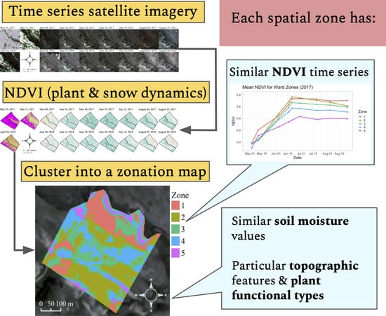
• The spatial zones—identified through hierarchical clustering of time series satellite imagery—are associated with distinct soil moisture distributions, plant functional types and topographic features.
• By comparing Ward and complete linkage methods of clustering, we found that the difference between the resulting zonation maps can be understood from the distance measures of these two linkages; the Ward method defined clusters with similar time series, which was more appropriate for our application, in contrast with the complete linkage method, which is more useful for extracting areas with extreme values.
• The zonation approach provides a tractable way to investigate ecosystem dynamics by structuring analysis and sampling efforts around spatial zones, where each zone represents a group with distinct plant-soil-snow interactions.

Based on these findings, we envision that sampling and analysis guided by this zonation approach will result in more effective use of time-lapse remote sensing data to capture the spatiotemporal variability of multiple system components—such as plants, snow and soil—across a landscape. This approach will provide opportunities to deepen understanding of ecosystem processes, identify their organization across space and time and predict how they will change in the future.

References

1. Lamanna, C.A. The Structure and Function of Subalpine Ecosystems in the Face of Climate Change. Ph.D. Thesis, University of Arizona, Tuscon, AZ, USA, 2012. [Google Scholar]
2. Sloat, L.L.; Henderson, A.N.; Lamanna, C.; Enquist, B.J. The Effect of the Foresummer Drought on Carbon Exchange in Subalpine Meadows. Ecosystems 2015, 18, 533–545. [Google Scholar] [CrossRef]
3. Wainwright, H.M.; Steefel, C.; Trutner, S.D.; Henderson, A.N.; Nikolopoulos, E.I.; Wilmer, C.F.; Chadwick, K.D.; Falco, N.; Schaettle, K.B.; Brown, J.B.; et al. Satellite-derived foresummer drought sensitivity of plant productivity in Rocky Mountain headwater catchments: Spatial heterogeneity and geological-geomorphological control. Environ. Res. Lett. 2020, 15, 084018. [Google Scholar] [CrossRef]
4. Diffenbaugh, N.S.; Scherer, M.; Ashfaq, M. Response of snow-dependent hydrologic extremes to continued global warming. Nat. Clim. Chang. 2013, 3, 379–384. [Google Scholar] [CrossRef] [PubMed] [Green Version]
5. Gerten, D.; Schaphoff, S.; Haberlandt, U.; Lucht, W.; Sitch, S. Terrestrial vegetation and water balance—hydrological evaluation of a dynamic global vegetation model. J. Hydrol. 2004, 286, 249–270. [Google Scholar] [CrossRef]
6. Fisher, J.B.; Malhi, Y.; Bonal, D.; Da Rocha, H.R.; De Araújo, A.C.; Gamo, M.; Goulden, M.L.; Hirano, T.; Huete, A.R.; Kondo, H.; et al. The land–atmosphere water flux in the tropics. Glob. Chang. Biol. 2009, 15, 2694–2714. [Google Scholar] [CrossRef]
7. Engstrom, R.; Hope, A.; Kwon, H.; Stow, D.; Zamolodchikov, D. Spatial distribution of near surface soil moisture and its relationship to microtopography in the Alaskan Arctic coastal plain. Hydrol. Res. 2005, 36, 219–234. [Google Scholar] [CrossRef]
8. Mohanty, B.P.; Skaggs, T.H.; Famiglietti, J.S. Analysis and mapping of field-scale soil moisture variability using high-resolution, ground-based data during the Southern Great Plains 1997 (SGP97) Hydrology Experiment. Water Resour. Res. 2000, 36, 1023–1031. [Google Scholar] [CrossRef] [Green Version]
9. Vereecken, H.; Huisman, J.A.; Pachepsky, Y.; Montzka, C.; van der Kruk, J.; Bogena, H.; Weihermüller, L.; Herbst, M.; Martinez, G.; Vanderborght, J. On the spatio-temporal dynamics of soil moisture at the field scale. J. Hydrol. 2014, 516, 76–96. [Google Scholar] [CrossRef]
10. Peng, J.; Loew, A.; Merlin, O.; Verhoest, N.E.C. A review of spatial downscaling of satellite remotely sensed soil moisture: Downscale Satellite-Based Soil Moisture. Rev. Geophys. 2017, 55, 341–366. [Google Scholar] [CrossRef]
11. Anderson, M.; Neale, C.; Li, F.; Norman, J.; Kustas, W.; Jayanthi, H.; Chavez, J. Upscaling ground observations of vegetation water content, canopy height, and leaf area index during SMEX02 using aircraft and Landsat imagery. Remote Sens. Environ. 2004, 92, 447–464. [Google Scholar] [CrossRef]
12. Wang, L.; Qu, J.J.; Hao, X.; Zhu, Q. Sensitivity studies of the moisture effects on MODIS SWIR reflectance and vegetation water indices. Int. J. Remote Sens. 2008, 29, 7065–7075. [Google Scholar] [CrossRef]
13. Hubbard, S.S.; Gangodagamage, C.; Dafflon, B.; Wainwright, H.; Peterson, J.; Gusmeroli, A.; Ulrich, C.; Wu, Y.; Wilson, C.; Rowland, J.; et al. Quantifying and relating land-surface and subsurface variability in permafrost environments using LiDAR and surface geophysical datasets. Hydrogeol. J 2013, 21, 149–169. [Google Scholar] [CrossRef]
14. Dafflon, B.; Oktem, R.; Peterson, J.; Ulrich, C.; Tran, A.P.; Romanovsky, V.; Hubbard, S.S. Coincident aboveground and belowground autonomous monitoring to quantify covariability in permafrost, soil, and vegetation properties in Arctic tundra. J. Geophys. Res. Biogeosci. 2017, 122, 1321–1342. [Google Scholar] [CrossRef] [Green Version]
15. Falco, N.; Wainwright, H.; Dafflon, B.; Léger, E.; Peterson, J.; Steltzer, H.; Wilmer, C.; Rowland, J.C.; Williams, K.H.; Hubbard, S.S. Investigating Microtopographic and Soil Controls on a Mountainous Meadow Plant Community Using High-Resolution Remote Sensing and Surface Geophysical Data. J. Geophys. Res. Biogeosci. 2019, 124, 1618–1636. [Google Scholar] [CrossRef] [Green Version]
16. Planet Team. Planet Application Program Interface: In Space for Life on Earth; Planet: San Francisco, CA, USA, 2017. [Google Scholar]
17. Wainwright, H.M.; Dafflon, B.; Smith, L.J.; Hahn, M.S.; Curtis, J.B.; Wu, Y.; Ulrich, C.; Peterson, J.E.; Torn, M.S.; Hubbard, S.S. Identifying multiscale zonation and assessing the relative importance of polygon geomorphology on carbon fluxes in an Arctic tundra ecosystem. J. Geophys. Res. Biogeosci. 2015, 120, 788–808. [Google Scholar] [CrossRef]
18. Dirmeyer, P.A.; Gao, X.; Zhao, M.; Guo, Z.; Oki, T.; Hanasaki, N. GSWP-2: Multimodel Analysis and Implications for Our Perception of the Land Surface. Bull. Am. Meteorol. Soc. 2006, 87, 1381–1398. [Google Scholar] [CrossRef] [Green Version]
19. Koster, R.D.; Guo, Z.; Yang, R.; Dirmeyer, P.A.; Mitchell, K.; Puma, M.J. On the Nature of Soil Moisture in Land Surface Models. J. Clim. 2009, 22, 4322–4335. [Google Scholar] [CrossRef] [Green Version]
20. Bergen, K.J.; Johnson, P.A.; de Hoop, M.V.; Beroza, G.C. Machine learning for data-driven discovery in solid Earth geoscience. Science 2019, 363, eaau0323. [Google Scholar] [CrossRef]
21. Hastie, T.; Tibshirani, R.; Friedman, J. The Elements of Statistical Learning: Data Mining, Inference, and Prediction, 2nd ed.; Springer: New York, NY, USA, 2009; ISBN 978-0-387-84858-7. [Google Scholar]
22. Reichstein, M.; Camps-Valls, G.; Stevens, B.; Jung, M.; Denzler, J.; Carvalhais, N. Prabhat Deep learning and process understanding for data-driven Earth system science. Nature 2019, 566, 195–204. [Google Scholar] [CrossRef]
23. Duda, T.; Canty, M. Unsupervised classification of satellite imagery: Choosing a good algorithm. Int. J. Remote Sens. 2002, 23, 2193–2212. [Google Scholar] [CrossRef]
24. Winkler, D.E.; Chapin, K.J.; Kueppers, L.M. Soil moisture mediates alpine life form and community productivity responses to warming. Ecology 2016, 97, 1553–1563. [Google Scholar] [CrossRef] [PubMed] [Green Version]
25. Hubbard, S.S.; Williams, K.H.; Agarwal, D.; Banfield, J.; Beller, H.; Bouskill, N.; Brodie, E.; Carroll, R.; Dafflon, B.; Dwivedi, D.; et al. The East River, Colorado, Watershed: A Mountainous Community Testbed for Improving Predictive Understanding of Multiscale Hydrological-Biogeochemical Dynamics. Vadose Zone J. 2018, 17, 180061. [Google Scholar] [CrossRef] [Green Version]
26. Kittel, G.; Rondeau, R.; Kettler, S. A classification of the riparian vegetation of the Gunnison River Basin, Colorado. In Submitted to Colorado Department of Natural Resources and the Environmental Protection Agency. Prepared by Colorado Natural Heritage Program, Fort Collins; Colorado State University: Ft. Collins, CO, USA, 1995. [Google Scholar]
27. PRISM Climate Group 30-Year Normals. Available online: https://prism.oregonstate.edu/normals/ (accessed on 4 July 2020).
28. Tucker, C.J. Red and Photographic Infrared Linear Combinations for Monitoring Vegetation. Remote Sens. Environ. 1979, 8, 127–150. [Google Scholar] [CrossRef] [Green Version]
29. Myneni, R.B.; Hall, F.G.; Sellers, P.J.; Marshak, A.L. The interpretation of spectral vegetation indexes. IEEE Trans. Geosci. Remote Sens. 1995, 33, 481–486. [Google Scholar] [CrossRef]
30. Hall, D.K.; Riggs, G.A. Normalized-Difference Snow Index (NDSI). In Encyclopedia of Snow, Ice, and Glaciers; Singh, V.P., Singh, P., Haritashya, U.K., Eds.; Encyclopedia of Earth Sciences; Springer: Dordrecht, The Netherlands, 2011; ISBN 978-90-481-2642-2. [Google Scholar]
31. Stillinger, T.; Roberts, D.A.; Collar, N.M.; Dozier, J. Cloud Masking for Landsat 8 and MODIS Terra Over Snow-Covered Terrain: Error Analysis and Spectral Similarity Between Snow and Cloud. Water Resour. Res. 2019, 55, 6169–6184. [Google Scholar] [CrossRef] [PubMed] [Green Version]
32. Chen, D.; Stow, D. The Effect of Training Strategies on Supervised Classification at Different Spatial Resolutions. Photogram. Eng. Remote Sens. 2002, 68, 1155–1162. [Google Scholar]
33. Millard, K.; Richardson, M. On the Importance of Training Data Sample Selection in Random Forest Image Classification: A Case Study in Peatland Ecosystem Mapping. Remote Sens. 2015, 7, 8489–8515. [Google Scholar] [CrossRef] [Green Version]
34. Breiman, L. Random Forests. Mach. Learn. 2001, 45, 5–32. [Google Scholar] [CrossRef] [Green Version]
35. Liaw, A.; Wiener, M. Classification and regression by randomForest. R News 2002, 2, 18–22. [Google Scholar]
36. Kassambara, A. Practical Guide to Cluster Analysis in R: Unsupervised Machine Learning; Multivariate Analysis; STHDA: Paris, France, 2017; Volume 1, ISBN 978-1-5424-6270-9. [Google Scholar]
37. Lawson, R.G.; Jurs, P.C. New index for clustering tendency and its application to chemical problems. J. Chem. Inf. Model. 1990, 30, 36–41. [Google Scholar] [CrossRef]
38. Dormann, C.F.; Elith, J.; Bacher, S.; Buchmann, C.; Carl, G.; Carré, G.; Marquéz, J.R.G.; Gruber, B.; Lafourcade, B.; Leitão, P.J.; et al. Collinearity: A review of methods to deal with it and a simulation study evaluating their performance. Ecography 2013, 36, 27–46. [Google Scholar] [CrossRef]
39. R Core Team. R: A Language and Environment for Statistical Computing; R Foundation for Statistical Computing: Vienna, Austria, 2019. [Google Scholar]
40. Ward, J.H. Hierarchical Grouping to Optimize an Objective Function. J. Am. Stat. Assoc. 1963, 58, 236–244. [Google Scholar] [CrossRef]
41. Wainwright, H.; Williams, K. LiDAR Collection in August 2015 over the East River Watershed, Colorado, USA; Lawrence Berkeley National Lab: Berkeley, CA, USA, 2017. [Google Scholar]
42. Zevenbergen, L.W.; Thorne, C.R. Quantitative analysis of land surface topography. Earth Surf. Process. Landforms 1987, 12, 47–56. [Google Scholar] [CrossRef]
43. Wilson, M.F.J.; O’Connell, B.; Brown, C.; Guinan, J.C.; Grehan, A.J. Multiscale Terrain Analysis of Multibeam Bathymetry Data for Habitat Mapping on the Continental Slope. Mar. Geod. 2007, 30, 3–35. [Google Scholar] [CrossRef] [Green Version]
44. Quinn, P.F.; Beven, K.J.; Lamb, R. The in(a/tan/β) index: How to calculate it and how to use it within the topmodel framework. Hydrol. Process. 1995, 9, 161–182. [Google Scholar] [CrossRef]
45. Falco, N.; Dafflon, B.; Devadoss, J.; Shirley, I.; Soom, F.; Uhlemann, S.; Wainwright, H.M. Time-domain reflectometer survey across the East River Watershed, Colorado. Watershed Funct. SFA 2020. [Google Scholar] [CrossRef]
46. Jones, S.B.; Wraith, J.M.; Or, D. Time domain reflectometry measurement principles and applications. Hydrol. Process. 2002, 16, 141–153. [Google Scholar] [CrossRef]
47. Dafflon, B.; Léger, E. Soil moisture and temperature data along the northeast facing hillslope at the Lower Montane site in the East River Watershed, Colorado. Watershed Funct. SFA 2020. [Google Scholar] [CrossRef]
48. Dietz, A.J.; Kuenzer, C.; Gessner, U.; Dech, S. Remote sensing of snow—A review of available methods. Int. J. Remote Sens. 2012, 33, 4094–4134. [Google Scholar] [CrossRef]
49. Chen, Y.; Wieder, W.R.; Hermes, A.L.; Hinckley, E.S. The role of physical properties in controlling soil nitrogen cycling across a tundra-forest ecotone of the Colorado Rocky Mountains, USA. CATENA 2020, 186, 104369. [Google Scholar] [CrossRef]
50. Harte, J.; Saleska, S.R.; Levy, C. Convergent ecosystem responses to 23-year ambient and manipulated warming link advancing snowmelt and shrub encroachment to transient and long-term climate-soil carbon feedback. Glob. Chang. Biol. 2015, 21, 2349–2356. [Google Scholar] [CrossRef] [PubMed]
51. Fisk, M.C.; Schmidt, S.K.; Seastedt, T.R. Topographic patterns of above- and belowground production and nitrogen cycling in alpine tundra. Ecology 1998, 79, 2253–2266. [Google Scholar] [CrossRef]
52. Zhang, T.; Zhang, Y.; Xu, M.; Zhu, J.; Chen, N.; Jiang, Y.; Huang, K.; Zu, J.; Liu, Y.; Yu, G. Water availability is more important than temperature in driving the carbon fluxes of an alpine meadow on the Tibetan Plateau. Agric. For. Meteorol. 2018, 256–257, 22–31. [Google Scholar] [CrossRef]
53. Walker, M.D.; Walker, D.A.; Theodose, T.A.; Webber, P.J. The Vegetation: Hierarchical Species-Environment Relationships. In Structure and Function of an Alpine Ecosystem: Niwot Ridge, Colorado; Bowman, W.D., Seastedt, T.R., Eds.; Oxford University Press: Oxford, UK, 2001; pp. 99–127. ISBN 978-0-19-511728-8. [Google Scholar]
54. Litaor, M.I.; Williams, M.; Seastedt, T.R. Topographic controls on snow distribution, soil moisture, and species diversity of herbaceous alpine vegetation, Niwot Ridge, Colorado. J. Geophys. Res. 2008, 113, G2. [Google Scholar] [CrossRef] [Green Version]
55. Körner, C. Alpine Plant Life: Functional Plant Ecology of High Mountain Ecosystems; Springer: Berlin, Germany, 2003; ISBN 978-3-540-00347-2. [Google Scholar]
56. Oroza, C.A.; Zheng, Z.; Glaser, S.D.; Tuia, D.; Bales, R.C. Optimizing embedded sensor network design for catchment-scale snow-depth estimation using LiDAR and machine learning. Water Resour. Res. 2016, 52, 8174–8189. [Google Scholar] [CrossRef] [Green Version]
57. Seddon, A.W.R.; Macias-Fauria, M.; Long, P.R.; Benz, D.; Willis, K.J. Sensitivity of global terrestrial ecosystems to climate variability. Nature 2016, 531, 229–232. [Google Scholar] [CrossRef] [Green Version]
58. Dong, C.; MacDonald, G.M.; Willis, K.; Gillespie, T.W.; Okin, G.S.; Williams, A.P. Vegetation Responses to 2012–2016 Drought in Northern and Southern California. Geophys. Res. Lett. 2019, 46, 3810–3821. [Google Scholar] [CrossRef]
Figure 1. The study area location in the context of the surrounding Colorado Rocky Mountains region.
Remotesensing 12 02733 g001
Figure 2. A portion of the time series of true color (RGB) satellite imagery with key dates in both years that show snow cover, plant growth, peak or near-peak plant productivity and senescence. Yellow lines outline the boundary between the north (left) and south (right) facing aspects. The full time series of images is included in the supplementary materials (Figure S1) along with the image IDs (Table S1). The coordinates displayed are NAD83, UTM zone 13N in meters.
Remotesensing 12 02733 g002
Figure 3. A time series of snowmelt on a rocky outcropping, with true color images (top), normalized difference vegetation index (NDVI) (middle) and snow classification results (bottom). Snow is not easily distinguishable from rock in true color images (top). Since snow is associated with low NDVI values, observations of an increase and subsequent stabilization of NDVI values (middle) throughout the growing season were used to identify the transition from snow to rock (bottom) when selecting training sites.
Remotesensing 12 02733 g003
Figure 4. Locations of 20 soil moisture sensors logging hourly volumetric water content from 1 June–10 August 2017 and 2018 and 60 one-time, point-probe time domain reflectometry (TDR) measurements taken on 2–3 July 2019. Each red point represents two TDR measurements.
Remotesensing 12 02733 g004
Figure 5. A true color image (left) compared with snow classification results (right) from PlanetScope satellite imagery of the East River watershed on 11 May 2017. Pixels classified as snow are displayed in pink.
Remotesensing 12 02733 g005
Figure 6. A portion of the time series of NDVI and snow classification from satellite imagery. Key dates in both years show snow cover, plant growth, peak or near-peak NDVI and senescence. Black lines outline the boundary between the north (left) and south (right) facing aspects. The full time series of images is included in the supplementary materials (Figure S2).
Remotesensing 12 02733 g006
Figure 7. Zonation maps based on (a) Ward and (b) complete linkage clustering methods. These zones are derived through clustering pixels, with a distinct NDVI time series associated with each pixel. Five clusters (corresponding to 5 spatial zones) were identified by the Ward method, while 7 clusters were identified by the complete linkage method.
Remotesensing 12 02733 g007
Figure 8. Temporal dynamics within each zone established by the (a) Ward method and (b) complete linkage method through clustering NDVI time series from satellite imagery. Error bars show the 99% confidence interval for the mean. Some error bars for very narrow confidence intervals appear as horizontal lines.
Remotesensing 12 02733 g008
Figure 9. A principal component analysis (PCA) biplot showing topographic variation within each spatial zone established by Ward method clustering of NDVI time series from satellite imagery. The length of each vector represents the loading of each variable (slope, curvature, Topographic Position Index, Topographic Wetness Index) on each Principal Component and the angle between each pair of vectors indicates the correlation between variables. Vectors with the same direction are positively correlated, while vectors with opposing directions are negatively correlated.
Remotesensing 12 02733 g009
Figure 10. The proportion of area covered by each plant functional type for each spatial zone derived from clustering NDVI time series from satellite imagery with the Ward method. Plant functional types were obtained from Falco et al. [15]. A table with the percent coverage of each plant functional type by zone is included in the supplementary materials (Table S4).
Remotesensing 12 02733 g010
Figure 11. Late spring snow presence and absence on May 11, 2017 and April 28, 2018 in relation to slope, elevation, aspect, topographic wetness index, topographic position index and curvature. Aspect is calculated here as the absolute angle from south (0) to north (180), with no distinction between east and west. The length of each vector represents the loading of each variable on each principal component and the angle between each pair of vectors indicates the correlation between variables. Vectors with the same direction are positively correlated, while vectors with opposing directions are negatively correlated. Ellipses show the distribution of each variable.
Remotesensing 12 02733 g011
Figure 12. Soil moisture as a function of zones derived from Ward method clustering of NDVI time series: (a) hourly continuously measured soil moisture sensor data at 50–60 cm depth (20 sensors) from June 1–August 10 in 2017 and 2018 and (b) one-time TDR point-probe measurements at 25 cm depth (60 locations) in July 2019. In (a), there were 3 sensors measuring hourly volumetric water content in Zone 1, 4 sensors in Zone 2, 5 sensors in Zone 3 and 8 sensors in Zone 4. Figure S3a,b displaying the time series of volumetric water content by zone are included in the supplementary materials. For the TDR measurements in (b), there were 2 samples taken in Zone 1, 20 in Zone 2, 20 in Zone 3, 16 in Zone 4 and 2 in Zone 5.
Remotesensing 12 02733 g012