OLCI A/B Tandem Phase Analysis, Part 2: Benefits of Sensors Harmonisation for Level 2 Products

Abstract

This study is a follow-up of a full methodology for the homogenisation and harmonisation of the two Ocean and Land Colour Instrument (OLCI) payloads based on the tandem phase analysis. Sentinel-3B was manoeuvred into a tandem configuration with its operational twin Sentinel-3A already in orbit few weeks after its launch, which was followed by a short drift phase during which Sentinel-3B was progressively moved to a specific orbit phasing of 140° separation from the sentinel-3A. Harmonisation is performed at Level 1 for the radiometric alignment of the OLCI-A TOA radiances to the ones of OLCI-B, considering the slight spectral differences between the two instruments. The benefits of this harmonisation for the main Level 2 products are assessed in the present manuscript for both land and water products. The results validate such benefits showing accuracy between the two sensors after harmonisation better than the products requirements specifications. For the water processing branch, this accuracy opens a path toward an ensemble Sentinel-3 system vicarious calibration with ground-truth measurements. For land products, the tandem phase analysis is also an opportunity to demonstrate that the terrestrial chlorophyll index product requires improvements of the preliminary spectral adjustment of the red-edge channel at 709 nm. As comparisons from the measurements acquired over the tandem phase provides confidence in the alignment of the OLCI-A and OLCI-B series of products, preliminary analysis of the measurements acquired over the drift phase provides the first insights into the sensitivity of the processing algorithms to the geometry of acquisition as well as to calibration residuals of the OLCI field-of-view. As the harmonisation currently performs a radiometric alignment of OLCI-A to OLCI-B, the question of the reference sensor for operational implementation of the harmonisation raises concerns on the individual quality of the calibration of each sensor, notably their across-track consistency. Following the investigations performed at Level 1, where relatively strong calibration residuals are shown between the OLCI cameras and very similarly for both instruments; we discuss the impact of these residuals at L2 using an empirical correction and further conclude with the need to address these problematics with more attention in the future. We conclude with the extreme usefulness of the tandem phase analysis, presently for Level 2 products, and the need to further monitor the temporal stability of the cross-calibration of the OLCI payloads with a view to implementing their harmonisation at operational level.

1. Introduction

A meaningful long-term environmental monitoring can only be ensured by the highest quality information. To provide this quality, the Copernicus Space Component (CSC) is continuously provided a fleet of dedicated satellites, the Sentinels, for the retrieval of essential climate variables. Sentinel-3, of the European Space Agency, is one of these satellites [1], providing data continuity for the historical ERS (all acronyms are provided in Abbreviations), ENVISAT, and elements of the PROBA and SPOT satellites, thanks to state-of-the-art payloads: the Ocean and Land Colour Instrument (OLCI), the Sea and Land Surface Temperature Radiometer (SLSTR), the SAR radar altimeter, and the microwave radiometer (MWR). Sentinel-3 includes two identical satellites flying on-orbit with 140° phase separation to provide global observations daily at the same equator crossing time and meet requirements. At the time of writing, Sentinel-3A and Sentinel-3B have been launched and replacement Sentinel-3C and Sentinel-3D satellites are completing their development.

A few weeks after its launch in April 2018, the European Commission Copernicus Sentinel-3B satellite was manoeuvred into a tandem configuration with its identical operational twin Sentinel-3A satellite already in orbit. A dedicated tandem calibration phase was conducted in which both satellites were flown only thirty seconds apart on the same orbit ground track. This approach limits the impact of ocean and atmosphere variability and results in acquisitions over the same targets with the same geometrical conditions. The Sentinel-3A/B tandem phase lasted from early June to mid October 2018 and provided a unique opportunity to increase knowledge of payload differences, homogenise datasets by defining appropriate adjustments, and to reduce uncertainties when comparing data. It was followed by a short drift phase during which the Sentinel-3B satellite was progressively moved to a specific orbit phasing of 140° separation from the sentinel-3A satellite.

The drift phase provides the opportunity to compare measurements acquired from the two sensors at differing viewing angles but only a few minutes apart (i.e., still with close illumination geometry and target condition) as sketched in Figure 1.

This article is a follow-up of a homogenisation and harmonisation methodology for the two OLCI-A and OLCI-B payloads described in [2]. Homogenisation first adjusts the slight spectral and spatial differences of the two sensors to provide comparable radiance measurements. The comparison of such homogenised L1 radiances acquired during the tandem phase provided evidence of radiometric biases of 1–2% between the two sensors, OLCI-A radiances being found higher than the ones of OLCI-B. These comparisons provided cross-calibration coefficients allowing the harmonisation of the two L1 products, OLCI-A being presently harmonised to OLCI-B for the sake of this study.

Although validation of the harmonisation has been conducted at Level 1 [2], notably through performing an ad hoc internal reprocessing of the tandem phase data, its benefits can only be fully addressed at subsequent levels (L2 and L3 presently). These products are the relevant inputs for scientific investigations such as disseminated by the dedicated Copernicus Land and Marine services (see, for instance, [3] for Copernicus Marine Environmental Monitoring Service (CMEMS) products). Consistency between the L2 and L3 products are therefore most critical for the OLCI mission continuity, regardless of the platform (OLCI-A and OLCI-B in the present analysis, OLCI-C, and OLCI-D in the future). We neither provide comparisons to ground truth nor provide quantitative comparisons between OLCI and other instruments of similar category (e.g., MODIS, VIIRS). Rather, the investigations of this study are presented with a view to assess the benefits of the harmonisation of the OLCI sensors for operational needs, which includes allowing a joint ocean colour system vicarious calibration of the Sentinel-3 mission as well as feeding multi-mission requirements for land monitoring and ocean colour communities.

The OLCI instrument, the main L2 scientific products along with their specifications are described. The datasets and levels of products used throughout this analysis are presented. Comparisons of tandem and drift phase are then analysed per type of target (land then water products). Whereas comparisons from tandem phase acquisitions show the benefit of the radiometric alignment on the L2 products, comparisons from drift phase acquisitions rely on the confidence obtained on the alignment to assess the geometrical stability of the products.

The discussion section handles the question of the reference sensor and a preliminary assessment of performing flat-fielding (i.e., equalisation of the independent OLCI cameras) of the radiometry, independently for each sensor as suggested in [2]. Conclusions are drawn toward the extreme usefulness of the tandem phase, presently for OLCI L2 and L3 products, and the operational applicability of the adjustments performed throughout this study provided the temporal stability of the OLCI-A/OLCI-B cross-calibration relationships.

2. OLCI Level 2 Scientific Products and Their Specifications

OLCI [4] is a multi-spectral imaging spectrometer acquiring in the visible (VIS) to near-infrared (NIR) domain (400–1020 nm) dedicated to ocean and land colour science at medium resolution (300 m full resolution, 1.2 km reduced resolution). In the continuity of ESA’s MEdium Resolution Imaging Spectrometer (MERIS), it is a good candidate to become a reference instrument for the radiometry in the VNIR, thanks to its advanced on-board calibration devices, wide swath and medium spectral resolution [4]. More description of the instrument and its calibration are provided in [2], we only recall that the coverage of the OLCI across-track (ACT) swath is achieved thanks to the combination of five independent cameras.

Contrary to OLCI L1 radiance products, L2 operational production is split between land and water branches operated under the responsibility of ESA and EUMETSAT (European Organisation for the Exploitation of Meteorological Satellites) respectively. Both L2 processing chains however share the same software and inputs (L1 products as well as characterisation and calibration database), starting the processing commonly for both branches by radiance-to-reflectance conversion, target classification and cloud screening, then eventually gaseous and smile-corrections. The processing then splits into two separate branches and pursues with dedicated algorithms.

Figure 2 sketches the flow of the L2 processing (eluding cloud screening and classification being made explicit by branch separation) considered in this manuscript with main inputs, transiting parameters, algorithms, and products. Internal aggregation to L3 is also performed by compositing a selection of L2 products on a daily basis (see below for details) and connected to the L2 process as depicted in the figure.

More description of the water branch can be found in [5]. Further details of the products are provided below per target.

2.1. L2 Land Products and Their Specifications

OLCI land processing inherits from the MERIS algorithms adapted to OLCI. It includes the OLCI global vegetation index (OGVI) and the OLCI terrestrial chlorophyll index (OTCI) inheriting respectively from the MGVI [6] and MTCI [7] algorithms. The OGVI is related to the fraction of absorbed photosynthetically active radiation (FAPAR) whereas the OTCI is related to canopy chlorophyll content. The Global Climate Observation System (GCOS) has identified FAPAR as an essential climate variable (ECV) [8].

The OGVI algorithm uses a parametric bidirectional reflectance factor model to account for the dependency of the TOA signal to geometrical conditions of observation and illumination across the field-of-view (FOV). The bidirectional reflectance model of [9] is optimized with respect to atmospheric, canopy, and soil characteristics from radiative transfer simulations of the surface-atmosphere coupling (see [6] for details). The OGVI directly uses TOA reflectances in blue (Oa03, 443 nm), red (Oa10, 681 nm), and NIR (Oa17, 865 nm) as well as the illumination (solar zenith and azimuth) and acquisition (viewing zenith and azimuth) angles.

Unlike the OGVI, the OTCI algorithm relies on the use of gas-, smile-, and Rayleigh-corrected reflectances (the so-called “top-of-aerosol” reflectances) in the red-edge, a spectral region situated between 680 and 750 nm, where the vegetation reflectance changes rapidly from an absorbing regime in the visible to a reflecting regime in the NIR ([10]). The following algorithm simply computes the ratio:

$$\mathrm{OTCI}=\frac{{\rho }_{754}-{\rho }_{709}}{{\rho }_{709}-{\rho }_{681}}$$

(1)

Performance requirements specifications can be traced from the early Sentinel-3 mission requirements [11] and can be summarised for both products as goal accuracy better than 5% at 0.3 km spatial resolution and threshold accuracy better than 10% at 1 km resolution.

2.2. L2 Water Products and Their Specifications

OLCI water processing also strongly inherits from the MERIS mission which has brought strong expertise in the field of ocean colour to Europe [12] following the launch of the carrying platform ENVISAT in 2002. The improvement of OC L2 products from OLCI is expected notably through the reduction of sun-glint contamination by imposing a viewing tilt (12.6° in the direction opposite to the Sun), the use of additional spectral bands (see [2] for a description of OLCI channels) dedicated to atmospheric corrections (Oa14, Oa15, Oa20, Oa21) and OC (Oa01, Oa09), as well as enhanced revisiting by combining multiple platforms (two payloads being the baseline).

The water processing relies firstly on the estimation of the aerosol loading (optical depth and type of aerosol) in the NIR and the propagation of its optical properties to the entire OLCI spectrum to correct the TOA signal for its atmospheric contribution and retrieval of the bottom-of-atmosphere (BOA) water-leaving reflectance [13]. Normalisation of this reflectance, computed at geometry of acquisition, to nadir-viewing zenith-illuminating geometry [14] is then a prerequisite for the estimation of the chlorophyll concentration (Chl) through the OC4Me algorithm [15]. This latter makes use of the maximum ratio ${}_j{}^{i}R$ between reflectances among either 443, 490, or 510 nm (Oa03 to Oa05), and reflectance at 560 nm (Oa06), combined to a polynomial fit of Chl concentration (in logarithm) as recalled below from [16].

$${\log }_{10}\left[\mathrm{Chl}\right]=a_0+{\Sigma }_{n=1}^N{a}_i{\left[{\log }_{10}\left({}_j{}^{i}R\right)\right]}^n \mathrm{where} {}_j{}^{i}R=\max \left(\frac{R\left(443\right)}{R\left(560\right)},\frac{R\left(490\right)}{R\left(560\right)},\frac{R\left(510\right)}{R\left(560\right)}\right)$$

Through the use of band ratios, Chl is less sensitive to radiometric uncertainties (see for instance §4.2.8.3 of [17]), however, changes in interband calibration (i.e., in the relative calibration of the OLCI channels) may impact the retrieved product.

Over the oceans, chlorophyll concentration appears over a wide dynamic range from about 0.01 to 30 mg·m^–3 (e.g., [3]) with a log-normal distribution. As explicated through this article, comparisons are addressed either in natural or log unit. Over the whole dynamic range, the use of relative differences as comparison figures is impacted by the dynamics of log(Chl) ranging between negative and positive values and crossing numerical singularity at “zero over zero”, natural unit is therefore privileged in such case.

Operational products discussed in this study include the directional water-leaving reflectance and Chl. Other products, not considered here, are notably elaborated for the monitoring of coastal waters (see [5] for details). The GCOS has identified water-leaving radiance and chlorophyll as ECVs [8] and expressed user requirements with ground truth as water-leaving radiance accuracy of 5% and ocean chlorophyll accuracy of 30%.

As providing a requirement in reflectance unit makes more sense than providing those in radiance unit, we consider that such requirements apply to water-leaving reflectances and not only to water-leaving radiances. Temporal stability requirements for chlorophyll are discussed in [18].

In this study, we can however only validate the relative accuracy between the OLCI-A and the OLCI-B products, the accuracy of an OLCI “system of systems” being firstly dependent on matching the user requirements between all OLCI sensors (A and B sensors presently). The absolute validation of the accuracy of the OLCI products is performed routinely through mission monitoring activities.

Notably, a system vicarious calibration (SVC) of the Level 2 water products can compensate some inaccuracies of the Level 1 calibration as well as biases induced by the processing models. One could therefore assume that inter-calibration of Level 2 products is not an issue after performing SVC. The situation is however more complex, as explicated below.

2.3. L2 Water Products System Vicarious Calibration and its Implications for Harmonisation

Contrary to land processing, water processing absolute calibration relies on an SVC which adjusts the sensor radiometry by offline comparisons with ground-truth measurements [19,20]. Since the late 1980’s SVC has been applied to OC sensors (e.g., [21,22]) notably to improve inter-mission consistency. SVC of OLCI (e.g., [23]) inherits from the methodologies developed and adapted from MERIS [24]. Currently, SVC of OLCI is computed from comparisons with MOBY [19], BOUSSOLE [20], and climatology of the water-leaving reflectance over oligotrophic oceanic regions. The ground reflectance reference is propagated to TOA, gas- and smile-corrected, reflectance for comparison to the OLCI adjusted reflectance. Per spectral channel, only one adjustment coefficient (i.e., one for all five cameras) is computed and assumed valid for the whole FOV and all observing conditions.

For OLCI-A, the current processing baseline considers vicarious gains whose effect is to decrease the radiometry of about 2% in the blue and progressively less toward red [23]. Adjustment in the NIR is performed in a first step and is only relative between all bands between 709 and 1020 nm to match aerosol spectral dependency. Adjustment in the VIS is performed in a second step; it is absolute although it relies on a proper adjustment of the NIR. Consequently, the OLCI SVC must be understood as the adjustment of a system combining the sensor radiometry and the L2 atmospheric correction models.

For OLCI-B, the operational baseline does not currently provide an SVC. Preliminary SVC, yet to be validated, has however been performed within the Sentinel-3 Mission Performance Centre (S3-MPC) and is considered for testing purposes (see next section). The OLCI-B SVC is performed similarly to the OLCI-A one.

Figure 3 compares the OLCI-A (baseline) and OLCI-B (preliminary and yet to validate) SVC gains. These independent SVCs may be used as a transfer calibration for the harmonisation of the two sensors, we have therefore added the gains corresponding to the radiometric alignment of OLCI-A to OLCI-B (i.e., following the convention in [2]) from the ratio of the two sets of SVC gains. Dispersions indicate the variability obtained from each assessment, standard deviation for the SVC-induced harmonisation is obtained from the two individual SVC coefficients through ${\sigma }_{harm}^2\left(\lambda \right)={\sigma }_{SVC-A}^2\left(\lambda \right)+{\sigma }_{SVC-B}^2\left(\lambda \right)$.

We first stress that the NIR gains are very close between the two SVCs despite the tandem analysis showing differences in the absolute calibration of about 1.5% in this spectral region [2]. This is because the SVC merely adjusts the spectral profile of the gains of the NIR bands without modifying the average absolute value. The inter-calibration differences between OLCI-A and OLCI-B propagate in the VIS through selecting different aerosol models and retrieving different aerosol optical thickness in the NIR. Consequently, the VIS calibration compensates these differences while also calibrating the system on absolute. The VIS gains show that OLCI-A requires a stronger adjustment than OLCI-B, especially in the blue region, corroborating the knowledge of OLCI-A being brighter than OLCI-B [25].

Whereas the SVC-derived harmonisation gains consequently corroborate these differences, these tend to be closer to zero when getting toward red and NIR. This does not correspond to the radiometric calibration differences highlighted by the L1 tandem analysis [2].

Figure 4 gives further details by similarly comparing the SVC-harmonisation gains with the mean harmonisation factors per camera (one colour per camera) obtained from the L1 tandem analysis [2]. Clearly, strong differences arise that we understand as caused by the lack of absolute calibration in the NIR within the SVC.

It is also to be noted that the dispersions obtained for the SVC gains in the VIS are larger than the maximum differences between harmonisation factors obtained for each camera (as well as much larger than the individual uncertainties of these factors). Such dispersions are related to the uncertainties arising from both the satellite and the ground-truth measurements (in situ or climatological database) but can also be attributable to mixing measurements from all cameras within the SVC gains assessment. We have indeed provided evidence [2] that all cameras show inter-calibration differences that can be up to 1.5–2% between cameras 4 and 5 (resp. for OLCI-A and OLCI-B) despite performing in-flight calibration.

Compared to tandem phase L1 harmonisation, these observations stress that SVC adjusts for the combined L1 calibration and L2 atmospheric correction. It does not replace cross-sensor calibration at L1, at least unless the NIR is first properly inter-calibrated between the sensors. However, it is well suited for the adjustments of L2 water products.

It is therefore interesting, as much as possible, to investigate water product comparisons between:

• OLCI-A with SVC and OLCI-B without SVC (current baselines)
• OLCI-A with SVC and OLCI-B with SVC (possible future baseline)
• OLCI-A without SVC, and radiometrically harmonised to OLCI-B, to OLCI-B without SVC (harmonised setup)

Currently, OLCI-A SVC is considered to be the most suited calibration setup through the validation of OLCI water products against ground truth measurements. We stress that the goal of this study is to provide insights on how to reach the best consistency between the OLCI products through sensor harmonisation, whatever post-calibration is applied next to align the products to ground-truth.

In the next section we define the datasets, data preparation, and levels of analysis, that are used throughout this study to achieve these investigations.

3. Datasets, Data Preparation, and Levels of Analysis

From the custom processing of a few small regions of interest to the collection of a large database, different levels of analysis are used throughout this article to compare the OLCI-A and OLCI-B products. We describe here the various datasets and their benefits for the analysis.

3.1. Datasets

As in [2], the datasets used in this work were collected in the frame of the Sentinel-3 Tandem for Climate project (s3tandem.eu), an ESA-funded project. The project data archive contains Sentinel-3A and Sentinel-3B data for all instruments, collected one day per week (Monday) between 25th June 2018 and 18th March 2019. This includes tandem (6th June 2018 to 15th October 2018), drift (22nd October 2018 to 19th November 2019), and post-tandem phases. More details on the project can be found in [26]. These “baseline” products were collected from the Payload Data Ground Segment (PDGS, land and marine centres).

In addition, an ad hoc internal reprocessing was performed on site along the duration of the S3TC project to provide a harmonised dataset (slightly reduced compared to the above one) based on the radiometric alignment of OLCI-A on OLCI-B presented in [2]. This reprocessed dataset does not consider flat-fielding corrections suggested in the conclusions of [2] as further improvements. The use of OLCI-B as reference was driven by radiometric validation activities suggesting that OLCI-A is too bright [25]. The harmonised OLCI-A products were generated using customised calibration gains for OLCI-A established from the product of the baseline OLCI-A calibration gains by the cross-calibration factors [2]. Moreover, no SVC has been applied to OLCI-A coherently with the baseline of OLCI-B for which SVC still needs to be validated.

The data archive contains L1B full resolution (FR) products, along with subsequent L2 products. Whereas only reduced resolution (RR) water baseline products were collected from the PDGS for the provision of the “baseline” database, both reduced and full resolution (FR) land and water products were processed and collected along the custom reprocessing for the provision of the “harmonised” dataset. In addition, few L2 processes, from a selection of L1B products, have been obtained for custom calibration setups (therefore mentioned as “custom” below), along with algorithm breakpoints (i.e., temporary/preliminary products) allowing more detailed analyses. This notably allows testing of various SVC setups for the comparison of water products.

3.2. Data Preparation and Additional L3 Composition

Like L1 products, OLCI-A and OLCI-B L2 products are originally subdivided into granules, elements of orbits corresponding to three minutes of acquisition. Pairs of co-located products are projected on a common latitude–longitude grid before comparisons (see [2] for details). The boundaries of such a grid encapsulate OLCI-A and OLCI-B products, any missing data from any sensor is discarded from the analysis.

This reprojection is performed similarly for all useful parameters, thanks to the L1B geolocation information: science products as well as the science quality flags necessary for target classification, quality screening, and rejection.

Aggregation to L3 is performed by compositing L2 products through reprojection on a plate carrée (equirectangular) grid of resolution 4 km × 4 km at Equator, daily averaging, and filtering for cloud contamination and sun-glint as well as standard quality flags.

Table 1. Datasets available for all categories of calibration setups: temporal sampling, product levels and types.

Product Level and Type	OLCI-A « Baseline »	OLCI-A « Harmonised »	OLCI-B « Baseline »	OLCI-A/OLCI-B « Custom »
Temporal sampling *	Full	Reduced	Full	A few scenes
L1	FR **	FR **	FR **	FR **
L2 Water (w/o SVC ***)	RR ** (SVC)	FR ** and RR ** (no SVC)	FR ** and RR ** (no SVC)	FR ** (any SVC)
L2 Land		FR ** and RR **	FR ** and RR **	FR **
L2 breakpoints				FR **
L3 Water	Daily mean	Daily mean	Daily mean
L3 Land	Daily mean	Daily mean	Daily mean

* Full: each Monday, reduced: selected Mondays; ** FR: full resolution, RR: reduced resolution; *** SVC: system vicarious calibration considered.

below provides a summary of the datasets available for all categories of calibration setups: temporal sampling, product levels, and types.

Missing data is either a consequence of unavailability within the data sources or due to a lack of concern when gathering the products for the study.

3.3. Levels of Analysis for the Comparisons

After reprojection to a common grid, pairs of L2 products allow direct pixel-wise comparisons. All L2 analyses are based on ACT statistics, which is allowed by the reprojection of the OLCI detector indices on the same grid as used for the other L2 products. Detector indices define the position of the pixel in the detector matrix where measurements were acquired, as each of the five cameras is made of 740 detectors/pixels, detector indices are numbered from 0 to 3699 corresponding to the total 3700 pixels over the full swath. We approximate the OLCI-A detectors to be roughly equal to the OLCI-B detectors for a common target on-ground, which is validated in [3]. Slight geolocation mismatches as well as instrumental and processing noise translate into dispersion in the comparisons.

We first base our analyses on a few dedicated scenes common to all the datasets, in other words, provided with any calibration setup. Four OLCI granules (two per target type), as cloud-free as possible, are selected among the tandem database to provide typical examples of water and land targets (see RGB images in Figure 5). For land, Amazonia (AMZ; 6.22° S, 62.66° W) and Europe (EUR; 46.20° N, 18.84° E) are selected to provide different vegetation types and degrees of homogeneity. For water, South Pacific Gyre (SPG; 17.08° S, 123.35° W) and Mediterranean Sea (MED; 36.01° N, 18.47° E) are selected for different chlorophyll concentrations and proportions of sun-glint contamination (no glint in SPG, unlike MED). Additional SVC setups are detailed in the water products comparisons section.

Then, statistics of L2 products (as much as possible from the baseline and harmonised datasets) confirm the observations made on these scenes from a larger statistics and covering a larger diversity of targets.

Drift phase comparisons are performed provided the two sensors’ footprints intersect over the same geographical area and are close enough temporally (at most a few minutes). This overlap is nearly complete during tandem [2] with measurements 30 s apart, increasingly limited during drift with delays of 3 and 9 min, respectively, on 22nd and 29th October 2018, which are the two sole dates available in the harmonised dataset.

Finally, L3 products have the advantage of providing a global, filtered and averaged, dataset representative of the final products dedicated to more synthetic information. It is convenient to compute statistics of the performance of the sensor harmonisation based on such products, notably to reduce impacts of instrumental noise.

Considering water products specifically, water-leaving reflectance is provided in the geometry of acquisition (i.e., directional). For drift phase comparisons, bidirectional reflectance distribution function (BRDF) correction is performed prior comparisons.

4. Results

In this section, we present all results separately for land and for water processing branches from the analysis of:

• Tandem phase comparisons over the selected L2 scenes
• Tandem phase statistics over L2 and L3 products
• Drift phase comparisons from L2 products

4.1. Land Products Comparisons and Analyses

4.1.1. OGVI Tandem Data Analysis

From the introduction of land products in Section 2, we understand that OGVI is much more sensitive to the absolute level of the TOA reflectance. This is first confirmed at L2 in Figure 6 showing OGVI relative difference statistics (median and median absolute deviation used to remove potential outliers) per OLCI detectors (bins of ten detectors used) for AMZ (left) and EUR (right).

The OGVI values are better aligned after harmonisation with very small relative differences (green lines). The results over Europe and Amazonia are similar, except for the higher dispersion for the Europe scene due to the larger inhomogeneity of the sampled vegetation covers.

The quality of the comparisons between the harmonised OLCI-A and OLCI-B products hold at L2 and L3 as shown below in Figure 7. L2 statistics are provided from a full day’s worth of statistics (e.g., 6th August 2018), gathering many different land targets. At L3, the compositing of L2 products into gridded daily averages lose track of the original ACT description of the observed variabilities so that we can no longer compare products along the FOV, comparisons are therefore shown as a function of OGVI.

From the L3 comparisons, OGVI mean (resp. median) relative difference between OLCI-A and OLCI-B are found to be 0.7% (resp. 0.0%), which is much better than the accuracy specifications.

4.1.2. OTCI Tandem Data Analysis

OTCI is more sensitive to the relative variations of the top-of-aerosol reflectance in the three spectral bands around the red-edge. As for OGVI, Figure 8 now shows OTCI relative difference statistics (median and median absolute deviation used to remove potential outliers) per OLCI detectors (bins of ten detectors used) for AMZ (left) and EUR (right). The OTCI values only show slight improvement in the comparisons between OLCI-A and OLCI-B after harmonisation.

These observations are confirmed over a day’s worth of L2 data statistics as well as at L3 where the comparisons suffer from mixing differences specific to each camera (Figure 9). On L3 comparisons, it is then no longer relevant to provide mean values with associated dispersions as the density distributions can be far from unimodal.

From the L3 comparisons, OTCI mean (resp. median) relative difference between OLCI-A and OLCI-B is found to be −1.2% (resp. −1.0%). On average, these figures are however better than the requirement specifications presented in Section 2.1.

Further analyses can be conducted to understand the discrepancies in OTCI. These analyses can be based on the breakpoints of the OTCI algorithm, for instance from the AMZ scenario (the same observations from EUR, not shown). Among these breakpoints, the top-of-aerosol reflectance of the Oa11 channel (709 nm) notably exhibits strong variability ACT (shown in Supplementary Figure S1), unlike the other spectral bands (not shown). We suspect this is because the red-edge is a region of strong reflectance gradient, especially at 709 nm close to the maximum red-edge gradient, and because the spectral response functions of the two instruments slightly differ (central wavelength differences reported in Figure S1, right). The OTCI algorithm is very sensitive to the accuracy in the reflectance at 709 nm as it is subtracted at numerator and added at denominator (we recall that $\mathrm{OTCI}=\left({\rho }_{754}-{\rho }_{709}\right)/\left({\rho }_{709}-{\rho }_{681}\right)$). In Figure S1, there are indeed across-track features in the two sets of differences that qualitatively compare (especially at camera 2), underlining this sensitivity.

However, the top-of-aerosol reflectances are supposed to be smile-corrected, in other words, adjusted to the same nominal channel around 709 nm. As this channel is very sensitive both to the red-edge spectral gradient and to water vapour absorption (moving the central wavelength ±1 nm changes H₂O absorption by 1% [27]), the main reason for observing such discrepancies is an inaccurate handling of the spectral adjustment. Indeed, smile-correction is performed by retrieving the reflectance gradient between 709 and 754 nm. This may not be the best choice and may not be accurate enough to correct tiny spectral differences.

For this purpose, we elaborate a sensitivity analysis based on the ECOSTRESS spectral library [28,29]. This database notably provides an extensive set of the spectral signature (albedo) of numerous vegetation species notably in the solar spectral range (VNIR and SWIR) with hyperspectral sampling (every 1 nm). Supplementary Figure S2 shows a subset of this database in the red-edge region. Many different spectral signatures exist, all providing lowest (resp. highest) reflectance around the red-edge at “boundary” channels 660–680 nm (resp. up to 750 nm) and inflexion points at various wavelengths between 690 and 720 nm (the so-called “red-edge position”, [7]), corroborating the choice of these specific channels in MERIS, OLCI, as well as many optical sensors designed for the monitoring of vegetation (e.g., Sentinel-2 MSI [30], FLEX [31]). The strong non-linearity of the spectral response makes it difficult to estimate the gradient by discrete differences.

Based on this dataset, we evaluate the ability to retrieve the spectral gradient at 709 nm by comparing, for each spectrum, the true gradient (computed locally from the hyperspectral data at exactly 709 nm) and the gradient estimated from a pair of channels combining either the 681 and 754 nm channels, or the 709 and 754 nm channels as originally performed (combining the 681 and 709 nm channels provides similar results to the latter and are not shown). Results are presented in Figure 10 with linear regression and coefficients of determination ($r^2)$.

Both results show that the estimated gradients nearly always underestimate the true value of the spectral gradient, the direct consequence being that smile effects (and therefore any small spectral difference between the sensors) will be under-corrected. Moreover, an estimation based on the two boundary channels (681 and 754 nm) is much better correlated to the exact value $\left(r^2=0.76\right)$ than the estimation based on the 709 and 754 nm channels $\left(r^2=0.39\right)$.

Applying the instrument spectral response functions (ISRFs) of OLCI-A and OLCI-B (available at https://sentinel.esa.int/web/sentinel/user-guides/sentinel-3-olci) on these datasets allows simulation of the correction of the BOA vegetation reflectance at 709 nm from the different combinations of channels presented above. For the 681/754 nm pair the benefit of using the additional fit for matching the exact reflectance gradient found in Figure 10 is also tested.

Statistics are derived independently for each sensor and from the collection of each vegetation spectrum. Relative differences between OLCI-A and OLCI-B estimated reflectance at 709 nm are shown in Figure 11 (mean and standard deviations obtained from all profiles of the ECOSTRESS database).

Whereas strong differences arise when combining any pair of channels, the use of the fit relating the estimated gradient from the 681/754 nm pair to the true gradient provides a significant improvement. We stress that this simulation, performed at BOA level and without geometrical dependency, does not handle the full features that come into play in the OLCI comparisons. Such a result however highlights the need to push forward with such simulations notably by including water vapour absorption, aerosols, and airmass (i.e., considering not only BOA spectra but rather quantities similar to the inputs of the OTCI algorithm) to investigate how to better align the estimation of the red-edge gradient on both OLCI sensors.

In conclusion, we suspect that the current estimation of the reflectance gradient in the red-edge is not accurate enough, discrepancies in the OTCI product between OLCI-A and OLCI-B will always persist as highlighted from the tandem data comparisons if no improvement of the smile-correction is addressed. This adds unnecessary uncertainties which can rise up to a few percent as seen in the L3 daily composites comparisons. Further work shall therefore consider correcting and validating the estimation of the red-edge gradient. Depending on the outcome of such work, recommendations could be to provide next Sentinel-3 generations with more channels within the red-edge (e.g., 720 nm). Synergy of Sentinel-3 with FLEX [31] shall also provide insights.

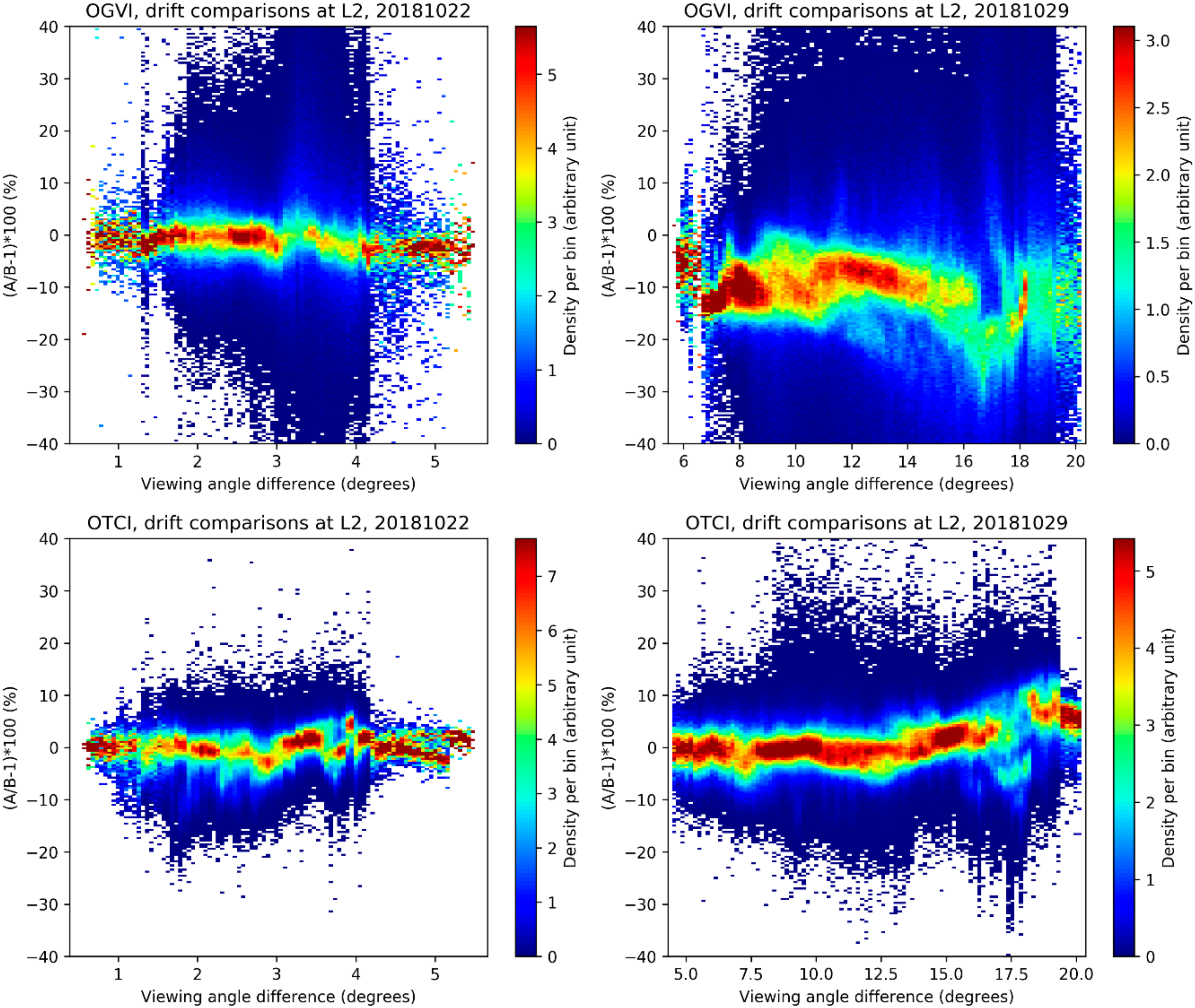
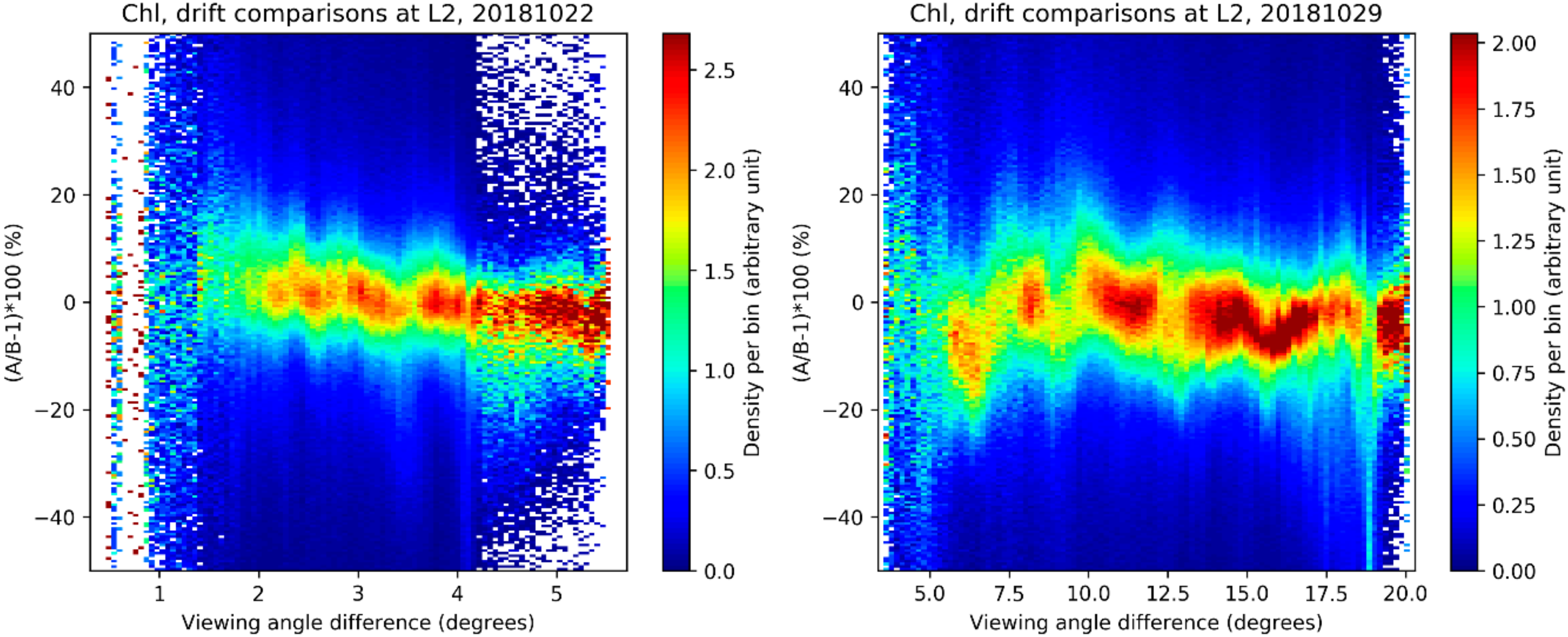
4.1.3. Drift Phase Data Analysis

During the drift phase the same targets are seen by the two sensors where the FOVs intersect with nearly equivalent illumination conditions but different viewing angles. We then compare the independently retrieved products as function of the differences in the viewing angles. All geometrical conditions are mixed in the statistics. Figure 12 shows statistics (density histograms) of the relative differences of OLCI-A and OLCI-B OGVI (top) and OTCI (bottom) as function of this viewing angle difference for the two drift dates available in the archive (left: 22nd October, 3 min apart; right: 29th October, 9 min apart).

Whereas slight differences on 22nd October can be attributed to per-detector sensitivity of the given parameter (especially for OTCI), more pronounced differences are seen on 29th October for larger viewing angle differences. OGVI seems less robust to changes in the viewing angle with about 10–20% relative differences even for relatively small angle differences (5°). This is probably due to the limitations of the models used to adjust the TOA signal to geometric conditions. On the contrary, OTCI, which is based on a ratio of reflectances from neighbouring bands, is more robust, a low angular dependency is observed in line with the sensitivity mentioned in [32].

4.2. Water Products Comparisons and Analyses

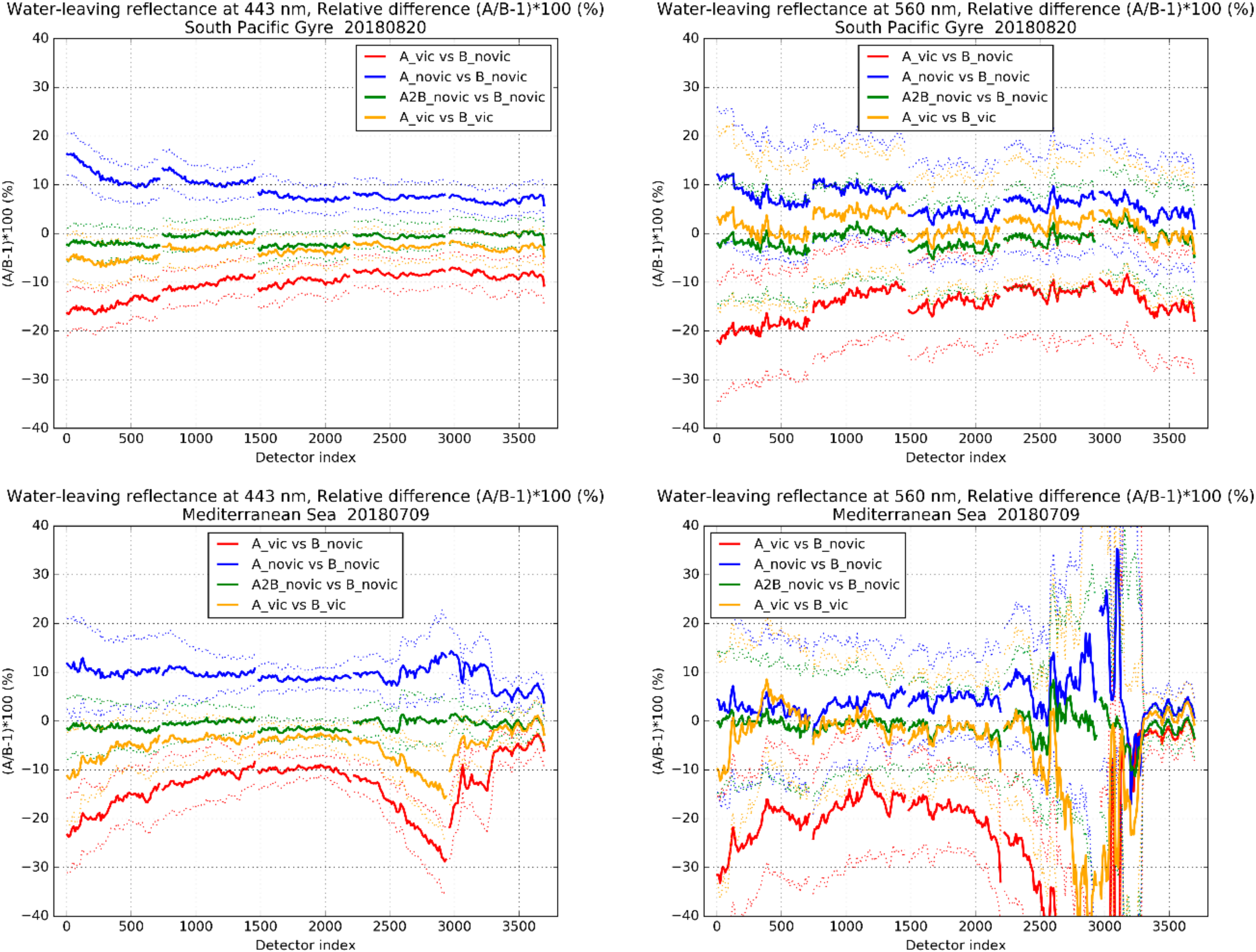
4.2.1. Tandem Data Analysis

The analysis of the SPG and MED scenes first provides a detailed insight into the relationships between OLCI-A water products with the OLCI-B ones using different calibration setups. OLCI-B is nominally processed without SVC (“B_novic” below), with which we have processed three versions of the OLCI-A products according to the three following calibration setups:

• No SVC and no alignment to OLCI-B (“A_novic”)
• SVC and no alignment to OLCI-B (“A_vic”)
• Alignment to OLCI-B and no SVC (“A2B_novic”)

In addition, the preliminary OLCI-B SVC (“B_vic”) is compared with the OLCI-A SVC to test the harmonisation of the products through independent SVCs, without L1 harmonisation.

Figure 13 for ${\rho }_w$ at 443 nm and 560 nm (resp. Oa03 and Oa06) and Figure 14 for Chl show the relative differences between OLCI-A and OLCI-B (taking this latter as the reference) for the different setups. Supplementary Figure S3 shows results for SPG for all bands from Oa01 (400 nm) to Oa06 (560 nm).

Following the order of the corrections being investigated, these comparisons show that:

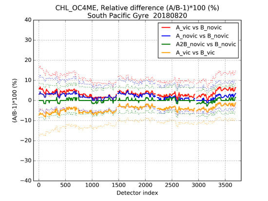
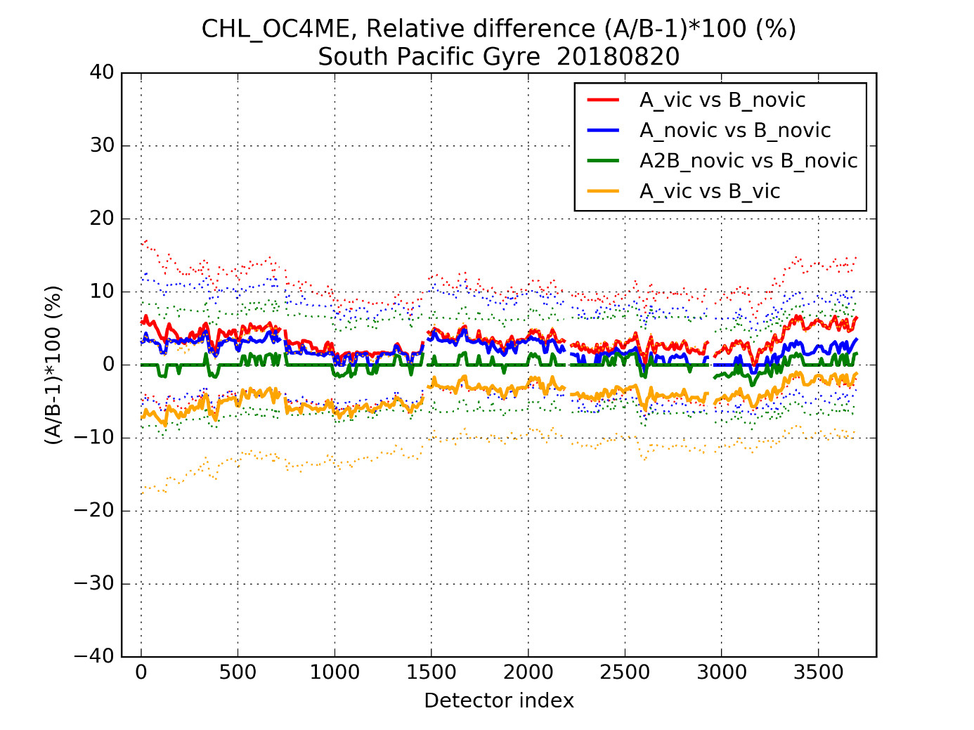
• A_novic and B_novic (blue lines) correspond to the initial response of the two sensors without any post-calibration (i.e., calibration additional to L1 calibration) applied. In the differences we see the impact of the relative higher brightness of OLCI-A compared to OLCI-B and its magnitude at BOA: 2% TOA differences translate into water-leaving reflectance differences up to about 10%. Interestingly, in cameras 1 and 2, differences, possibly accentuated by the high viewing angle, are large enough to propagate intra-camera calibration residuals (so-called “hat shapes” in [2]) which have been suspected to arise from stray light correction residuals.
• A_vic and B_novic (red lines) correspond to the current baseline with OLCI-A being adjusted through SVC. There, the initial over-brightness of OLCI-A is compensated, the effect being caused by a decrease of the OLCI-A radiometry according to SVC. We see here that this setting does not provide efficient alignment, which shows that an SVC of OLCI-B would benefit the comparison.
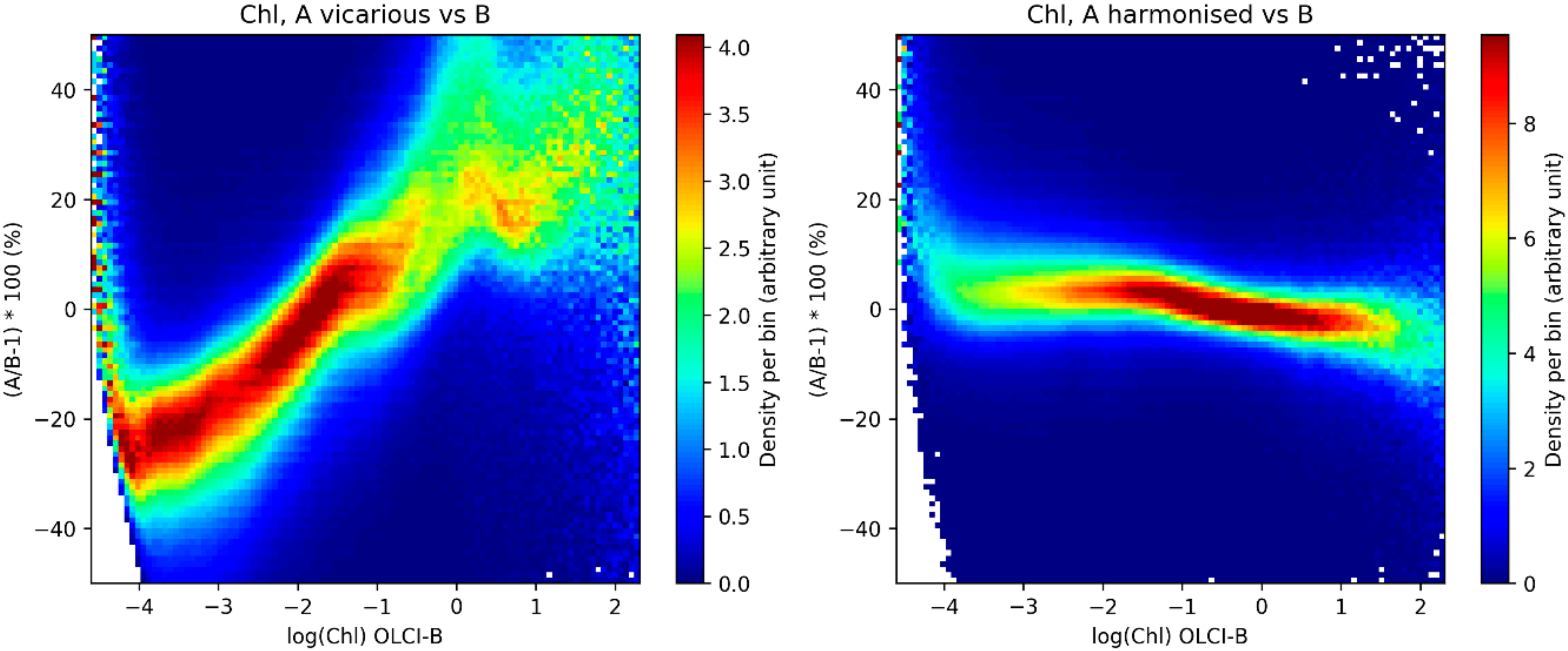
• A_vic and B_vic (yellow lines) indeed show the benefit of adjusting OLCI-B by SVC. However, the residual differences are not always centred around zero, especially for reflectance at 412 and 443 nm where specifications of 5% accuracy are not always met. Furthermore, the spectral consistency does not provide an alignment on the Chl product. Compared to SPG, the MED scenario is affected by sun-glint even though filtering has been performed.
• A2B and B_novic (green lines) now provide the best alignment, for water-leaving reflectance and for Chl, consistently with L1 harmonisation allowing OLCI-A to behave as a radiometric “copy” of OLCI-B. However, comparisons with ground-truth (not yet performed on this basis) would most probably underline the need of performing SVC on this harmonised dataset.

SVC-adjusted products are indeed most relevant for validation with ground-truth, and, therefore, should be the products to use from the Sentinel-3 OLCI operational production (however waiting for validation of OLCI-B SVC). However, the L1 harmonisation provides a much better alignment of the L2 water products and, most important, better spectral consistency between the datasets resulting in better comparisons of Chl products.

In the MED scenario, comparisons are strongly affected by sun-glint in the eastern portion of the FOV (detector index larger than 2000) so that the statistics there are provided by pixels that have gone through the filtering process but are close to glint conditions. The consequence is that the relationships between the two products are less stable ACT (also compared to the SPG scenario). The L1 harmonisation also provides the best consistency over this region.

These observations greatly favour L1 harmonisation before SVC is performed, either for each sensor individually or jointly for both sensors (see discussion section for more). This is underlined below by further comparing harmonised datasets over statistics of L2 and L3 products, and comparing the accuracy obtained with the mission specifications.

As for land targets, daily L2 statistics (e.g., from August 6th, 2018) of the relative differences between the harmonised products indeed corroborate the previous observations in Figure 15 for ${\rho }_w$ at 443 and 560 nm and Figure 16 for Chl (in natural unit). Supplementary Figure S4 provides complete results for all bands from Oa01 (400 nm) to Oa06 (560 nm).

There is clearly more noise at 560 nm than at 443 nm as the signal is smaller, the magnitude of noise on Chl differences consequently follows the magnitude of the latter. For reflectance, calibration residuals appear through slight discontinuities at camera interfaces, especially at 400 nm where camera 3 is most sensitive (Figure S4). For Chl, band ratioing removes such effects as all Chl bands from Oa03 to Oa06 are affected by similar discontinuities (see again Figure S4).

At L3, the compositing of L2 products into gridded daily averages lose track of the original ACT description so that we can no longer compare along the FOV. Inter-camera residual differences are no longer visible. Moreover, aggregation into L3 products is accompanied by the BRDF correction of the reflectance into nadir-zenith geometry into so-called normalised remote-sensing reflectances (nRrs) that are among the nominal inputs for providing homogenised products for comparing various OC missions [3].

The provision of OLCI-A L2 (and then L3) water baseline and harmonised products allows comparing of the relationships between OLCI-A and OLCI-B reflectances in Figure 17 and Chl in Figure 18 (natural unit) for these two cases (see legends for details). Supplementary Figures S5 and S6 show the results for all bands from Oa01 to Oa06.

These figures show further evidence that the current baseline, without OLCI-B SVC, does not provide relevant accuracy for mission consistency between the two sensors. On the contrary, the radiometric alignment performed at L1 provides an excellent alignment of the L2 water products, for all bands and throughout the dynamics, with accuracy much better than 5% for ${\rho }_w$, still better than 5% for Chl, as summarised below in

Table 2. Mean and median relative differences (%) between harmonised OLCI-A and OLCI-B L2 water products from L3 comparisons.

Quantity	nRrs 400	nRrs 412	nRrs 443	nRrs 490	nRrs 510	nRrs 560	Chl
Mean relative difference (%)	−0.4	−1.2	0.3	0.9	1.0	1.6	4.0
Median relative difference (%)	−0.3	−1.4	-0.8	0.6	0.7	1.1	3.0

. Figures for Chl are provided in natural units as it is the unit in which the accuracy requirements are addressed.

These figures are much better than the accuracy specifications, leaving a comfortable margin for the exploitation of the L1 harmonisation for SVC as well as for analysis of the drift phase data.

4.2.2. Drift Phase Data Analysis

To compare water products from the drift phase acquisitions, normalisation is applied on the L2 water-leaving reflectance from the two available dates. As for land products, reprojection of the products handles the co-location of the products corresponding to the same target on the ground. Only harmonised datasets are relevant for such comparisons as explained in Section 3. Compared to land products, water reflectance accuracy relies more on the quality of the atmospheric corrections. The drift phase provides an efficient setup for the validation of the handling of the geometrical dependency of the atmospheric signal by the correction scheme employed in the OLCI processing.

Figure 19 for normalised water-leaving reflectance, and Figure 20 for Chl, show the relative differences between the OLCI-A and OLCI-B products as a function of the viewing angle difference between the two payloads.

Differences are on average roughly centred on zero for all products, even for the highest viewing angle differences, showing that the atmospheric corrections handle geometric effects in a relatively efficient manner. However, strong oscillations in the reflectance comparisons appear that can be due to imperfect equalisation of the cameras as well as mixing of various illumination conditions. Water reflectance is more sensitive to small calibration differences as their proportion in the total TOA reflectance is small. Chl being estimated from band ratios, this variable is less sensitive.

As for land products, these results show that this type of analysis would also benefit from a larger dataset based on the complete drift phase dataset. Potentially, a larger dataset could allow disentangling of the handling of the geometrical differences by the processing models from the residual impact of ACT calibration differences, leading to a better estimation of the model errors.

Compared to land products, ACT calibration differences have even more impact on the water products. We investigate the impact of such differences in the discussion below as well as quantify the benefits of performing flat-fielding.

5. Discussion: The Question of the Reference Sensor and the Potential Benefits of Flat-Fielding for L2 Products

It is an easier task to harmonise the sensors based on the tandem harmonisation information than to choose which sensor to use as reference. In [2] a discussion is held on the choice of the reference sensor for the harmonisation of OLCI-A and OLCI-B. Many radiometric validation assessments provide evidence that OLCI-A is too bright, while OLCI-B agrees better with other missions and simulations [25]. However, [2] provides significant insight on the need, for both OLCI sensors, to perform flat-fielding prior to any alignment of the sensors as both payloads exhibit inter-camera residual calibration biases. These residuals have not been addressed while producing all the datasets used in this study, and therefore reduce the quality of the comparisons based on the drift phase acquisitions as shown above.

To compensate the residuals, flat-fielding adjustment coefficients have been estimated in [2], individually for each sensor (see [2] for details). These coefficients are averages from a dispersion of results obtained individually for all channels, to the exception of strong absorption channels.

Table 3. Estimated flat-fielding adjustment coefficients for OLCI-A and OLCI-B from [2].

	Cam 1	Cam 2	Cam 3	Cam 4	Cam 5
OLCI-A	0.992	0.997	1.000	0.998	0.988
OLCI-B	0.991	0.997	1.000	0.996	0.983

recalls the coefficients retrieved in [2].

As we can see, differences are the largest between cameras 4 and 5 and then between cameras 1 and 2 with up to nearly 2% (resp. 1%) relative differences. Although these figures are within the radiometric performance specifications of OLCI [1], a simple comparison to the SVC figures underlines the necessity to pay more attention to this problem: even a change of a few percent in the radiometry can bring significant changes to L2.

In [2], the application of the coefficients of Table 3, prior harmonisation, allowed finding more consistent harmonisation coefficients between the OLCI cameras. A linear regression of the harmonisation factors with wavelength, independent of the camera, was provided as a first order relationship to align the flat-fielded radiometry of the sensors. We mention that camera 3 was found slightly outside this relationship at Oa06 (560 nm), a channel most important for chlorophyll retrieval, possibly because of sensitivity of ozone absorption to the wavelength of acquisition. Indeed, to the exception of strong absorption features, gaseous absorption is provided at the same nominal wavelength for both OLCI sensors, in other words, it does not handle slight spectral differences of the OLCI detectors.

As the relevance of radiometric flat-fielding gets its full importance at Level 2, we presently assess the benefits of performing this flat-fielding adjustment combined with assessing the use of the mean harmonisation relationship aligning the radiometry of OLCI-A to the one of OLCI-B as a linear function of the wavelength of acquisition. The goal here is two-fold: first, check that the mean relationship handles the harmonisation sufficiently since it is of much simpler use although it relaxes the accuracy of the harmonisation; second, investigate the benefits of flat-fielding.

To this end, we rely on specific processing of the scenarios described in Figure 5 using the following calibration setups:

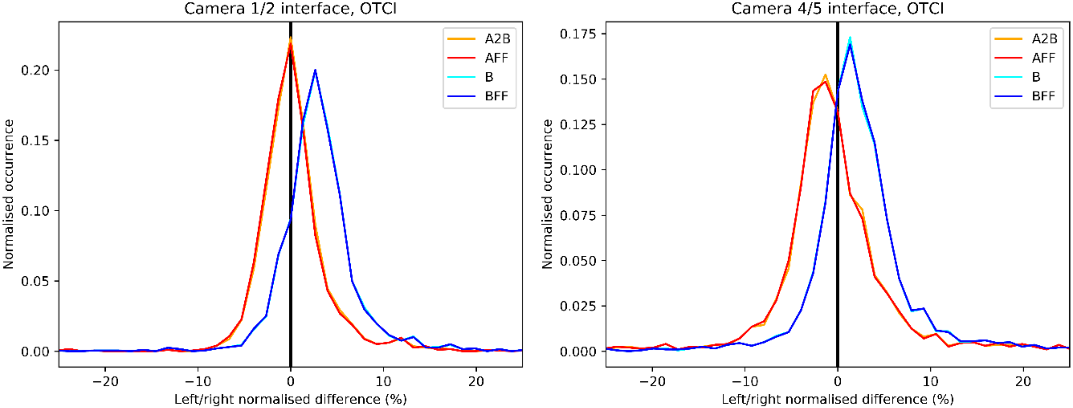
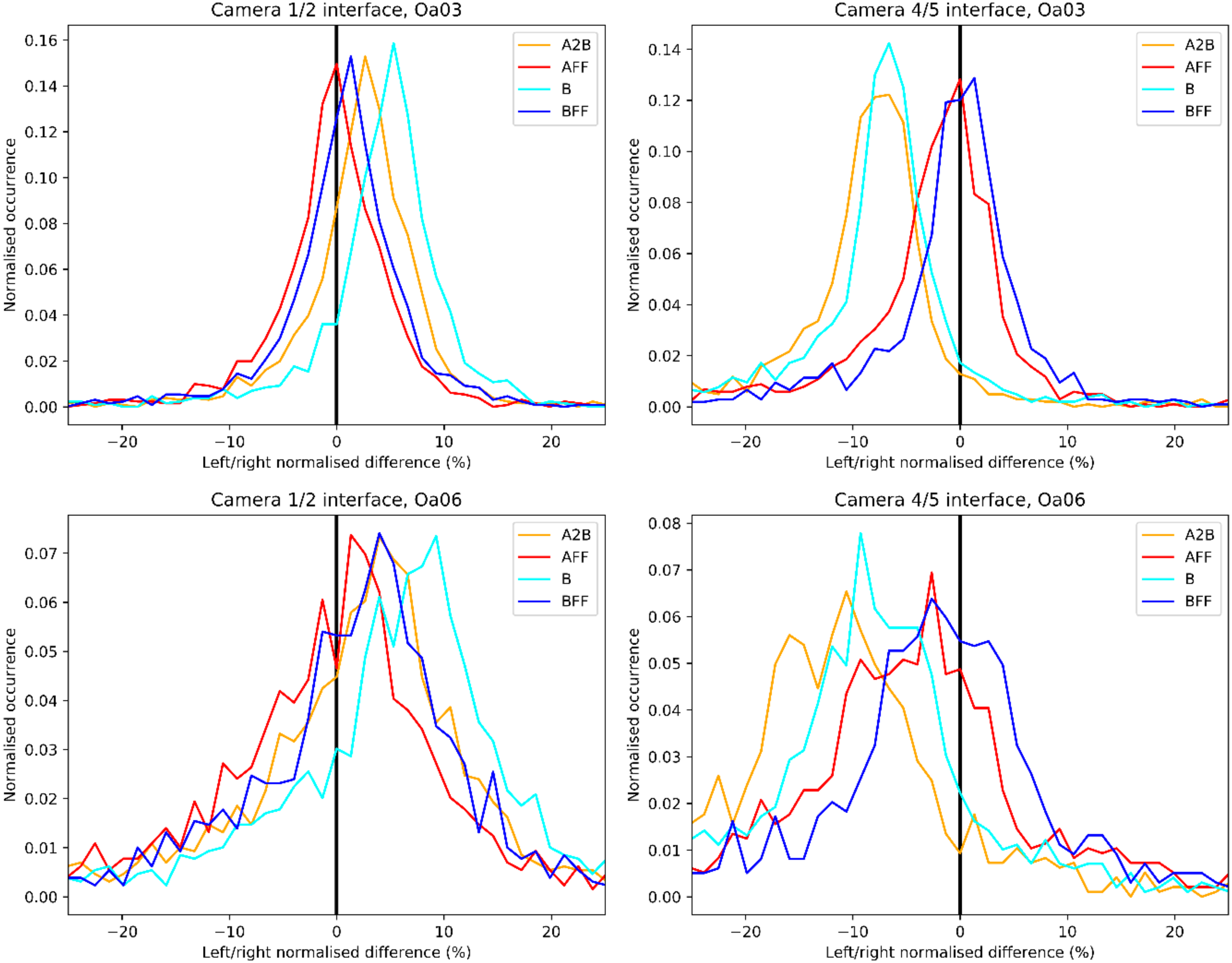
• OLCI-A harmonised to OLCI-B (“A2B”), as from the harmonised dataset
• OLCI-B (“B”), still taken as reference to “A2B”
• OLCI-A flat-fielded and harmonised to OLCI-B (flat-fielded as well) using the linear regression (“AFF”)
• OLCI-B flat-fielded (“BFF”) now taken as reference to “AFF”

First verification of the performance of the harmonisation of OLCI-A and OLCI-B, based on flat-fielded radiances, is made by comparing the alignment of the L2 products provided by these calibration setups with the ones using the full harmonisation (i.e., the harmonisation with full ACT dependency as used for the harmonised datasets). Corroborating our previous findings, Supplementary Figure S7 shows (over AMZ, not shown for EUR but similar results) that the harmonisation of OGVI performs with nearly equivalent quality using the two setups, whereas OTCI is still impacted by the slight spectral differences of the sensors.

For L2 water products, where the BOA signal is much more sensitive to changes in the absolute calibration, the slight relaxation of the harmonisation accuracy translates into relatively larger differences in the water-leaving reflectances (Figure S8) and then on chlorophyll (Figure S9, log unit used) showing results from SPG (qualitatively the same result from MED, not shown). These results show that, even though it is less reliable than the full harmonisation (especially at 560 nm), the mean harmonisation relationship still provides better alignment than the SVCs.

This however brings sufficient quality to assess the benefits of flat-fielding at L2; we then proceed separately for land and water products. As these benefits would appear through ACT consistency of a considered product, we rely on the most homogeneous scenarios which are provided from the AMZ scenario for land (restricted to a section of the image where homogeneous vegetation covers the complete FOV), and the SPG scenario for water (also restricted to a region with mostly homogeneous Chl).

We first analyse averages of the L2 products along the along-track (ALT) dimension as discontinuities of the considered parameters are sought within the ACT dimension. Then, a closer look at the interfaces of the cameras, where the products should be continuous, provides statistics for the differences between the mean values obtained for each camera of their respective interface. Results are shown individually for the four calibration setups: A2B and AFF setups are shown in (resp.) orange and red, B and BFF setups are shown in (resp.) cyan and blue.

5.1. Benefits of Flat-Fielding for Land Products

Figure 21 shows the ALT-averages for OGVI (left) and OTCI (right) obtained over AMZ, as function of the detector index.

Strong ACT variability is firstly most probably due to the fact that the vegetation cover cannot be considered as homogeneous as originally assumed. At camera interfaces, and especially between cameras 1/2 and 4/5, there are more continuous OGVI values for the calibration setups which include flat-fielding. On the contrary, ACT-continuity in OTCI, when considering flat-fielding or not for each of the sensors, rather shows that the differences are directly due to the spectral differences of the cameras (and of the cameras of the two sensors). In both cases, these effects can hardly be disentangled from the natural ACT variability which sometimes exhibits variations of the same magnitude as the one found at the camera interfaces.

Performing statistics for differences at camera interfaces then provides a more efficient analysis. Figure 22 for OGVI and Figure 23 for OTCI show the statistics of the normalised differences between the values obtained from the two adjacent cameras of interfaces 1/2 (left) and 4/5 (right) where flat-fielding is the most impacting (complete results for all interfaces in Supplementary Figures S10 and S11).

For OGVI, the benefits of performing flat-fielding appear clearly at interface 4/5 (less but slightly at interface 1/2) where mean biases of about 2% (resp. 1%) are cancelled out. For OTCI, the results confirm there is no change when applying flat-fielding for each instrument as discrepancies are rather due to the ACT spectral differences.

These results show that flat-fielding provides a benefit for OGVI with a maximum improvement in the order of 2% between cameras 4 and 5 corresponding to the alignment of the L1 TOA radiances of the same magnitude. This figure must be compared to the 5% accuracy specification of OGVI: we understand that about half of this accuracy is lost if not correcting the inter-camera calibration residuals.

5.2. Benefits of Flat-Fielding for Water Products

Following the same methodology for water products (SPG scenario), Figure 24 first shows the ALT-averages for water-leaving reflectance at 443 nm (left) and 560 nm (right) obtained over SPG. Results for all bands between 400 and 560 nm are qualitatively comparable and are not shown.

The absolute differences between OLCI-A and OLCI-B (with or without flat-fielding) first corroborate the differences from Figure S8. Whereas camera 3 values for OLCI-B remain unchanged after flat-fielding (which we recall uses camera 3 as reference), these values for OLCI-A change between the A2B and AFF setups, and especially significantly at 560 nm (orange vs. red curves). This corroborates the observation, recalled above, that the cross-calibration of camera 3 at 560 nm is slightly outlying the linear regression found between AFF and BFF used to harmonise the OLCI-A and OLCI-B radiometry in this context.

Anyway, what is most striking are the strong reflectance discontinuities of the order of 5–10% magnitude at camera interfaces 1/2 and 4/5 obtained from the nominal A2B and B calibration setups compared to the flat-fielded products. Contrary to land products, these discrepancies can more easily be attributable to calibration artefacts as their magnitude stands out against than the natural variability out of camera interfaces.

Similarly as for land products, this is further confirmed by computing the normalised relative differences at the camera interfaces as shown in Figure 25, restricted to interfaces 1/2 and 4/5. Results for all bands and all interfaces are synthesized in Supplementary Figure S12 showing only the median values obtained from the distributions along with their dispersion.

In all cases, OLCI-A flat-fielded statistics provide more centred differences (red vs. orange lines). For OLCI-B, the benefits appear rather at interfaces 1/2 and 4/5 than at interface 2/3, where differences are more centred for B (i.e., not flat-fielded), and at interface 3/4 where results are comparable between B and BFF. We also mention that geophysical variability (i.e., not perfectly homogeneous interface) and instrumental noise induce width in the distributions.

Last but not least, the impact on Chl is expected to be low as the flat-fielding performs equally on all bands and as the OC4ME Chl algorithm relies on ratioing either reflectance at 443, 490, or 510 nm with reflectance at 560 nm. Figure 26 indeed shows that, although discontinuities of Chl can be found between cameras, these are not removed through considering flat-fielding.

The corresponding analysis of the normalised relative differences at the camera interfaces shown in Figure S13 further confirms that residual biases are found between the cameras, individually for OLCI-A and for OLCI-B, which are not affected by flat-fielding. These residual biases may be related to the sensitivity of the algorithm to the precision of the reflectance notably through ozone absorption correction (which we recall does not handle the full ISRFs dependency) and to slightly different interband calibration (i.e., relative radiometric alignment of the bands) between the cameras. These effects are however of minor amplitude compared to the target specification requirements. We finally note the larger dispersion of the distributions compared to the ones obtained from the reflectances.

5.3. Conclusion of the Discussion

In conclusion, we have provided a preliminary demonstration of the potential benefits of performing flat-fielding prior harmonisation of the OLCI sensors. Flat-fielding here provides better ACT consistency to OGVI, and much more effectiveness to the water-leaving reflectance. The level of accuracy of the flat-fielding coefficients is therefore primarily driven by the requirements of ocean colour which must be addressed in priority. Although OC4ME Chl is not benefiting directly from such adjustment, other OC algorithms may not be as robust with such calibration differences.

The main concern that we raise is the sensitivity of ocean colour to even tiny calibration differences. If no flat-fielding is performed at L1, SVC must handle the slightly different calibration of the cameras. We however recommend, for the sake of mission consistency, that all harmonisation and flat-fielding adjustments be performed similarly for all processing branches, in other words, prior to any L2 processing.

More investigations must however fully validate the approach: first for the determination of the flat-fielding coefficients (as preconised by [2]) and then for the confirmation of its benefits from wider statistics than just a few acquisitions.

6. Conclusions and Way Forward

The Sentinel-3 Tandem phase is an extremely significant experiment. Following the assessment of its benefits for OLCI L1 radiometry, we have presently assessed the many potential benefits for the OLCI L2 products. The tandem phase notably allows conducting of very fine sensitivity analyses of the algorithms with slight spectral and radiometric differences that indeed impact the two sensors.

We have verified that the harmonisation of the L1 radiometry of the OLCI-A and OLCI-B sensors provides the best reachable alignment of the L2 products. For land products, the benefit for OGVI has proven very significant whereas persistent differences in OTCI have allowed understanding of the necessity for performing more accurate smile-correction in the red-edge. Simulations from BOA vegetation spectra provide an assessment of potential improvements of this correction.

For water products, the L1 harmonisation provides an excellent accuracy in the alignment of L2 water-leaving reflectance and chlorophyll compared to mission requirements, opening the way for a potential joint OLCI system of systems vicarious calibration. Indeed, although harmonisation performs the best possible radiometric alignment of the two payloads, both need to be calibrated against absolute references. Such vicarious calibration could be validated through comparisons to fiducial measurements and to other OC sensors (MODIS/VIIRS for instance).

The reliability of the harmonisation, demonstrated from the comparisons over the tandem phase acquisitions, allowed a preliminary assessment of the benefits obtained from the analysis of the drift phase acquisitions. Indeed, this configuration allowed testing the sensitivity of the various algorithms and models to changes in geometry as the same targets are seen by the two harmonised sensors from different viewing angles. First, comparisons underline the current limitations of the products, notably for OGVI where significant differences are found for viewing angle differences larger than 10°. These results show that this type of analysis would benefit from a larger dataset, ideally over the complete drift phase dataset (and not only two days out of this drift phase as is presently available). An extended dataset would notably allow disentangling effects due to the sampling of different types of vegetation cover, different illumination conditions, as well as inter-camera calibration residuals.

Pursuing the discussion elaborated for L1 radiometry, it appears that most L2 products (especially water products and OGVI) would potentially benefit from the flat-fielding (i.e., equalisation of the radiometry of the cameras) of each of the OLCI sensors. We have demonstrated this benefit over a few data samples, notably by showing water-leaving reflectance differences up to 10% being cancelled after applying flat-fielding. Although full validation of the approach needs to be conducted, such adjustment opens the way to better consistency of the OLCI products for the Sentinel-3 mission and we consider these aspects as a priority in the near future.

As these analyses are performed from the tandem and drift phases, it is finally of great importance to monitor the OLCI cross-calibration throughout the mission lifetime. Insights of the temporal stability of the radiometric differences between OLCI-A and OLCI-B as well as the inter-camera radiometric differences for each sensor are assessed in a following study.

References

1. Donlon, C.; Berruti, B.; Buongiorno, A.; Ferreira, M.-H.; Féménias, P.; Frerick, J.; Goryl, P.; Klein, U.; Laur, H.; Mavrocordatos, C.; et al. The Global Monitoring for Environment and Security (GMES) Sentinel-3 mission. Remote Sens. Environ. 2012, 120, 37–57, ISSN 0034-4257. [Google Scholar] [CrossRef]
2. Lamquin, N.; Clerc, S.; Bourg, L.; Donlon, C. OLCI A/B Tandem Phase Analysis, Part 1: Level 1 Homogenisation and Harmonisation. Remote Sens. 2020, 12, 1804. [Google Scholar] [CrossRef]
3. Garnesson, P.; Mangin, A.; Fanton d’Andon, O.; Demaria, J.; Bretagnon, M. The CMEMS GlobColour Chlorophyll-a Product Based on Satellite Observation. Ocean Sci. Discuss. 2019, 1–16. [Google Scholar] [CrossRef]
4. Nieke, J.; Borde, F.; Mavrocordatos, C.; Berruti, B.; Delclaud, Y.; Riti, J.-B.; Garnier, T. The Ocean and Land Colour Imager (OLCI) for the Sentinel 3 GMES Mission: Status and first test results. In Proceedings of the SPIE 8528, Earth Observing Missions and Sensors: Development, Implementation, and Characterization II, 85280C, Kyoto, Japan, 28 November 2012. [Google Scholar] [CrossRef]
5. EUMETSAT. Sentinel-3 OLCI Marine User Handbook; EUM/OPS-SEN3/MAN/17/907205; EUMETSAT: Darmstadt, Geramny, 2018. [Google Scholar]
6. Gobron, N.; Pinty, B.; Verstraete, M.; Govaerts, Y. The MERIS global vegetation index (MGVI): Description and preliminary application. Int. J. Remote Sens. 1999, 20, 1917–1927. [Google Scholar] [CrossRef]
7. Dash, J.; Curran, P.J. The MERIS terrestrial chlorophyll index. Int. J. Remote Sens. 2004, 25, 5403–5413. [Google Scholar] [CrossRef]
8. The Global Observing System for Climate: Implementation Needs. GCOS-200, GOOS-214. 2016. Available online: https://library.wmo.int/doc_num.php?explnum_id=3417 (accessed on 30 May 2020).
9. Rahman, H.; Pinty, B.; Verstraete, M.M. Coupled surface± atmosphere reflectance (CSAR) model. 2. Semiempirical surface model usable with NOAA Advanced Very High Resolution Radiometer data. J. Geophys. Res. 1993, 98, 20791–20801. [Google Scholar] [CrossRef]
10. Horler, D.N.H.; Dockray, M.; Barber, J. The Red Edge of Plant Leaf Reflectance. Int. J. Remote Sens. 1983, 4, 273–288. [Google Scholar] [CrossRef]
11. Drinkwater, M.R.; Rebhan, H. Sentinel-3 Mission Requirements Document. Ref: EOP-SMO/1151/MD-md. 2007. Available online: http://esamultimedia.esa.int/docs/GMES/GMES_Sentinel3_MRD_V2.0_update.pdf (accessed on 30 May 2020).
12. Bézy, J.L.; Delwart, S.; Rast, M. MERIS—A new generation of ocean-colour sensor onboard Envisat. August 2000. ESA bulletin. Eur. Space Agency 2000, 103, 48–56. [Google Scholar]
13. Antoine, D.; Morel, A. A multiple scattering algorithm for atmospheric correction of remotely-sensed ocean colour (MERIS instrument): Principle and implementation for atmospheres carrying various aerosols including absorbing ones. Int. J. Remote Sens. 1999, 20, 1875–1916. [Google Scholar] [CrossRef]
14. Morel, A.; Gentili, B. Diffuse reflectance of oceanic waters. II Bidirectional aspects. Appl Opt. 1993, 32, 6864–6879. [Google Scholar] [CrossRef] [PubMed]
15. Antoine, D. OLCI Level 2 Algorithm Theoretical Basis Document: Ocean Colour Products in Case 1 Waters; Ref S3-L2-SD-03-C10-LOVATBD. 2010. Available online: https://www.eumetsat.int/website/home/Satellites/CurrentSatellites/Sentinel3/OceanColourServices/index.html (accessed on 30 May 2020).
16. Morel, A.; Huot, Y.; Gentili, B.; Werdell, P.J.; Hooker, S.B.; Franz, B.A. Examining the consistency of products derived from various ocean color sensors in open ocean (Case 1) waters in the perspective of a multi-sensor approach. Remote Sens. Environ. 2007, 111, 69–88. [Google Scholar] [CrossRef]
17. IOCCG. Uncertainties in Ocean Colour Remote Sensing; Mélin, F., Ed.; IOCCG Report Series, No. 18; International Ocean Colour Coordinating Group: Dartmouth, NS, Canada, 2019. [Google Scholar] [CrossRef]
18. Hammond, M.L.; Henson, S.A.; Lamquin, N.; Clerc, S.; Donlon, C. Assessing the effect of Tandem Phase Sentinel 3 OLCI sensor uncertainty on the estimation of potential ocean chlorophyll trends. Remote Sens. 2020, 12, 2522. [Google Scholar] [CrossRef]
19. Brown, S.W.; Flora, S.J.; Feinholz, M.E.; Yarbrough, M.A.; Houlihan, T.; Peters, D.; Kim, Y.S.; Mueller, J.; Johnson, B.C.; Clark, D.K. The marine optical buoy (MOBY) radiometric calibration and uncertainty budget for ocean colour satellite sensor vicarious calibration. In Proceedings of the SPIE on Optics & Photonics, Sensors, Systems, and Next-Generation Satellites XI, Florence, Italy, 17–20 September 2007. [Google Scholar]
20. Antoine, D.; Guevel, P.; Deste, J.F.; Bécu, G.; Louis, F.; Scott, A.J.; Bardey, P. The BOUSSOLE buoy-a new transparent-to-swell taut mooring dedicated to marine optics: Design, tests, and performance at sea. J. Atmos. Ocean. Technol. 2008, 25, 968–989. [Google Scholar] [CrossRef]
21. Gordon, H.R. Calibration requirements and methodology for remote sensors viewing the ocean in the visible. Remote Sens. Environ. 1987, 22, 103–126. [Google Scholar] [CrossRef]
22. Franz, B.A.; Bailey, S.W.; Werdell, P.J.; McClain, C.R. Sensor-independent approach to the vicarious calibration of satellite ocean color radiometry. Appl. Opt. 2007, 46, 5068–5082. [Google Scholar] [CrossRef] [PubMed]
23. Lamquin, N.; Bourg, L.; Lerebourg, C.; Martin-Lauzer, F.-R.; Kwiatkowska, E.; Dransfeld, S. System Vicarious Calibration of Sentinel-3 OLCI. In Proceedings of the Calibration Conference (CALCON) Proceedings, Logan, Utah, 23 August 2017. [Google Scholar]
24. Lerebourg, C.; Mazeran, C.; Huot, J.P.; Antoine, D. Vicarious Adjustment of the MERIS Ocean Colour Radiometry; ESA/ESRIN MERIS ATBD-2.24 Issue 1.0; ESA: Frascati, Italy, 2011. [Google Scholar]
25. Bourg, L.; Blanot, L.; Alhammoud, B.; Sterck, S.; Preusker, R. Sentinel-3 A and B OLCI instruments Calibration Status. In Proceedings of the Fifth Sentinel-3 Validation Team Meeting, Frascati, Italy, 7–9 May 2019. [Google Scholar]
26. Clerc, S.; Donlon, C.; Borde, F.; Lamquin, N.; Hunt, S.E.; Smith, D.; McMillan, M.; Mittaz, J.; Woolliams, E.; Hammond, M.; et al. Benefits and Lessons Learned from the Sentinel-3 Tandem Phase. Remote Sens. 2020, 12, 2668. [Google Scholar] [CrossRef]
27. Fischer, J.; Preusker, R.; Lindstrot, R. Sentinel-3 OLCI Gaseous Correction Algorithm Theoretical Baseline Document. Ref SE-l2-SD-03-C03-FUB-ATBD_GaseousCorrection. 2010. Available online: https://sentinel.esa.int/documents/247904/349589/OLCI_L2_ATBD_Gaseous_Correction.pdf (accessed on 30 May 2020).
28. Meerdink, S.K.; Hook, S.J.; Roberts, D.A.; Abbott, E.A. The ECOSTRESS spectral library version 1.0. Remote Sens. Environ. 2019, 230, 1–8. [Google Scholar] [CrossRef]
29. Baldridge, A.M.; Hook, S.J.; Grove, C.I.; Rivera, G. The ASTER Spectral Library Version 2.0. Remote Sens. Environ. 2009, 113, 711–715. [Google Scholar] [CrossRef]
30. Frampton, W.J.; Dash, J.; Watmough, G.; Milton, E.J. Evaluating the capabilities of Sentinel-2 for quantitative estimation of biophysical variables in vegetation. ISPRS J. Photogramm. Remote Sens. 2013, 82, 83–92. [Google Scholar] [CrossRef] [Green Version]
31. Drusch, M.; Moreno, J.; Del Bello, U.; Franco, R.; Goulas, Y.; Huth, A.; Kraft, S.; Middleton, E.M.; Miglietta, F.; Moammed, G.; et al. The FLuorescence EXplorer Mission Concept—ESA’s Earth Explorer 8. IEEE Trans. Geosci. Remote Sens. 2017, 55, 1273–1284. [Google Scholar] [CrossRef]
32. Dash, J.; Vuolo, F. OLCI Terrestrial Chlorophyll Index (OTCI) Algorithm Theoretical Basis Document. Ref S3-L2-SD-03-C14UoS-ATBD_OTCI. 2010. Available online: https://sentinel.esa.int/documents/247904/349589/OLCI_L2_ATBD_OLCI_Terrestrial_Chlorophyll_Index.pdf (accessed on 30 May 2020).
Figure 1. Sketch of the differences between tandem and drift phase geometry. Sentinel-3 platform image by SkywalkerPL (https://commons.wikimedia.org/w/index.php?curid=47012912).
Remotesensing 12 02702 g001
Figure 2. Sketch of the OLCI L2/L3 processing for land and water branches with emphasis on the main algorithms and products used in this analysis.
Remotesensing 12 02702 g002
Figure 3. Comparison between the current OLCI-A (red/orange) and preliminary OLCI-B (blue/cyan) SVC gains, and a tentative set of SVC harmonisation gains (black/grey) along with associated dispersions. Gains at 1020 nm falls out of the scale and are not considered.
Remotesensing 12 02702 g003
Figure 4. Comparison between the mean harmonisation factors per camera (one colour per camera) from [2] and the tentative set of SVC harmonisation gains along with their dispersion (black for VIS absolute gains, grey for NIR relative gains), gain at 1020 nm falls out of the scale and is not considered.
Remotesensing 12 02702 g004
Figure 5. RGB images of the selected scenes for L2 full resolution comparisons: Amazonia and Europe (top) for the land branch, South Pacific Gyre and Mediterranean Sea (bottom) for the water branch.
Remotesensing 12 02702 g005
Figure 6. OGVI relative differences of OLCI-A baseline (“A”, red) and harmonised (“A2B”, green) with OLCI-B for Amazonia (left) and Europe (right). Median and dispersion per OLCI detector.
Remotesensing 12 02702 g006
Figure 7. (Left): OGVI relative differences of harmonised OLCI-A and OLCI-B over one day statistics (20180806). Results are shown as histograms per bin of OLCI detector. Medians and dispersions added in plain (resp. dashed) lines. (Right): the same but computed from all L3 composites over the tandem period. Results are shown as histograms per value of OGVI with OLCI-B taken as reference.
Remotesensing 12 02702 g007
Figure 8. OTCI relative differences of OLCI-A baseline (“A”, red) and harmonised (“A2B”, green) with OLCI-B for Amazonia (left) and Europe (right). Median and dispersion per OLCI detector.
Remotesensing 12 02702 g008
Figure 9. (Left): OTCI relative differences of harmonised OLCI-A and OLCI-B over one day statistics (20180806). Results are shown as histograms per bin of OLCI detector. Medians and dispersions added in plain (resp. dashed) lines. (Right): the same but computed from all L3 composites over the tandem period. Results are shown as histograms per value of OTCI with OLCI-B taken as reference.
Remotesensing 12 02702 g009
Figure 10. Relationships between exact red-edge reflectance gradient at 709 nm and its estimate from the ratio of the reflectance at two OLCI bands: 709/754 nm (left) and 681/754 nm (right). Datasets from the ECOSTRESS spectral library [28,29]. Linear regression presented along with coefficient of determination.
Remotesensing 12 02702 g010
Figure 11. Relative differences between estimations of the vegetation reflectance at 709 nm using OLCI-A and OLCI-B ISRFs (plain lines) using two pairs of channels (709/754 nm and 681/754 nm), in green is used the fit from Figure 10. Simulations based on the ECOSTRESS spectral library [28,29]. Dashed lines indicate standard deviation.
Remotesensing 12 02702 g011
Figure 12. Relative differences of OLCI-A and OLCI-B OGVI (top) and OTCI (bottom) as function of the viewing angle difference for the two drift dates available in the archive (left: 22nd October, 3 min apart; right: 29th October, 9 min apart). Density histograms are made per viewing angle bin (size adapted to the case).
Remotesensing 12 02702 g012
Figure 13. Relative differences of OLCI-A and OLCI-B water-leaving reflectance (Oa03, 443 nm, left: Oa06, 560 nm, right) for South Pacific Gyre (top) and Mediterranean Sea (bottom). OLCI-A processed with three calibration setups when compared to OLCI-B without SVC: no SVC and no alignment (blue), SVC (red), alignment to OLCI-B (green). In yellow, OLCI-A with SVC compared to OLCI-B with preliminary SVC. Median and dispersion per OLCI detector. Eastern part of the FOV affected by sun-glint in the MED scenario.
Remotesensing 12 02702 g013
Figure 14. Relative differences of OLCI-A and OLCI-B Chl (log unit) for South Pacific Gyre (left) and Mediterranean Sea (right). OLCI-A processed with three calibration setups: no SVC and no alignment (blue), SVC (red), alignment to OLCI-B (green). Median and dispersion per OLCI detector. Eastern part of the FOV affected by sun-glint in the MED scenario.
Remotesensing 12 02702 g014
Figure 15. Relative differences of harmonised OLCI-A and OLCI-B water-leaving reflectance (Oa03, 443 nm, left; Oa06, 560 nm, right) over one day statistics (20180806). Results are shown as histograms per bin of OLCI detector.
Remotesensing 12 02702 g015
Figure 16. Relative differences of harmonised OLCI-A and OLCI-B Chl (natural unit) over one day statistics (20180806). Results are shown as histograms per bin of OLCI detector.
Remotesensing 12 02702 g016
Figure 17. Normalised remote-sensing reflectance (Oa03, 443 nm, top; Oa06, 560 nm, bottom) relative differences between OLCI-A (baseline, left; harmonised, right) and OLCI-B from all L3 composites over the tandem period. Results are shown as histograms per bin of the corresponding parameter with OLCI-B taken as reference.
Remotesensing 12 02702 g017
Figure 18. Chl (natural unit) relative differences between OLCI-A (left: baseline, right: harmonised) and OLCI-B from all L3 composites over the tandem period as a function of Chl (log unit to embrace the full dynamics). Results are shown as histograms per bin of the corresponding parameter with OLCI-B taken as reference.
Remotesensing 12 02702 g018
Figure 19. Relative differences of OLCI-A and OLCI-B water-leaving reflectance at 443 nm as function of the viewing angle difference for the two drift dates available in the archive (left: 22nd October, 3 min apart; right: 29th October, 9 min apart). Density histograms are made per viewing angle bin.
Remotesensing 12 02702 g019
Figure 20. Relative differences of OLCI-A and OLCI-B chlorophyll as function of the viewing angle difference for the two drift dates available in the archive (left: 22nd October, 3 min apart; right: 29th October, 9 min apart). Density histograms are made per viewing angle bin.
Remotesensing 12 02702 g020
Figure 21. ALT-averages of OGVI (left) and OTCI (right) over AMZ for the four calibration setups.
Remotesensing 12 02702 g021
Figure 22. OGVI normalised relative differences between the values obtained from the two adjacent cameras for interface 1/2 (left) and interface 4/5 (right) and for the four calibration setups. Flat-fielding efficiently reduces differences of OGVI at camera interfaces.
Remotesensing 12 02702 g022
Figure 23. OTCI normalised relative differences between the values obtained from the two adjacent cameras of interface 1/2 (left) and interface 4/5 (right) and for the four calibration setups. Flat-fielding is not sufficient to reduce differences between A and B at camera interfaces, highlighting their origin in spectral rather than radiometric differences.
Remotesensing 12 02702 g023
Figure 24. ALT-averages of water-leaving reflectance at Oa03 (443 nm, left) and Oa06 (560 nm, right) over SPG for the four calibration setups.
Remotesensing 12 02702 g024
Figure 25. Water-leaving reflectance (Oa03, left; Oa06 right) normalised relative differences between the values obtained from the two adjacent cameras of interface 1/2 (left) and interface 4/5 (right) for the four calibration setups. Inter-camera differences are efficiently reduced with flat-fielding.
Remotesensing 12 02702 g025
Figure 26. ALT-averages of chlorophyll over SPG for the four calibration setups.
Remotesensing 12 02702 g026