An Improved Frequency-Domain Image Formation Algorithm for Mini-UAV-Based Forward-Looking Spotlight BiSAR Systems

Abstract

Mini-unmanned aerial vehicle (UAV)-based bistatic forward-looking synthetic aperture radar (SAR) (mini-UAV-based BFSAR) is much more attractive than the monostatic one because of the flexibility of the system geometry selection as well as its simplicity of system operation, especially with the mini-UAV platform. However, the trajectory of the mini-UAV needs to be accurately modeled since it is very sensitive to the external environment, and the forward-looking configuration results in more severe spatial variance in image formation processing. In the paper, an improved frequency-domain imaging algorithm based on a very accurate slant range model is proposed for mini-UAV-based BFSAR with spotlight illumination. First, a more accurate slant range expression considering the motion characteristics of the UAV and bistatic spotlight configuration is re-derived. Second, a new range nonlinear chirp scaling (NLCS) operator was derived based on the accurate bistatic slant range model. Third, an improved azimuth NLCS operator in the Doppler frequency domain was established for the spotlight illumination of the transmitter and receiver in mini-UAV based BFSAR systems. Finally, the proposed algorithm is validated by both simulations and real datasets.

1. Introduction

Synthetic aperture radar (SAR) [1,2] has become a very attractive technique because it can provide high-resolution images during the day and night regardless of weather conditions. However, in the forward-looking case, monostatic SAR cannot achieve high-resolution imaging along the azimuth direction because it cannot form an effective Doppler bandwidth, and mirror effects also occur in this scenario. To solve these difficulties, bistatic forward-looking SAR (BFSAR) has been introduced as a working mode, in which the receiver adopts forward-looking and spotlight reception while the transmitter adopts broadside or squint illumination to simultaneously form an effective Doppler bandwidth and avoid mirror effects [3,4,5,6,7,8,9,10,11]. On the other hand, mini unmanned aerial vehicles (mini-UAVs) have been adopted by radar engineers as the carriers of SAR due to their flexibility and ease of deployment, especially for some new applications such as aircraft self-landing, material airdrops, terrain awareness and avoidance [12]. By combining the mini UAV and BFSAR concepts, this paper deals with the image formation of mini-UAV-based spotlight BFSAR systems.

Despite the above-mentioned advantages of such a system, mini-UAVs are very sensitive to the outer environment, such as wind, and accurate image formation is therefore one of the most important issues for mini-UAV-based BFSAR. A large amount of literature has been dedicated to the image formation algorithm for a variety of BiSAR systems. The back-projection (BP) algorithm is a theoretically accurate image formation algorithm for any SAR system, but it is limited by its inefficiency [13,14,15].

Chirp scaling (CS) and nonlinear CS (NLCS) algorithms have been widely adopted in SAR image formation since they achieve a good compromise between the accuracy and the efficiency of the algorithms [16,17,18,19,20,21,22,23,24,25,26]. To deal with the complex bistatic range of BiSAR, most CS and NLCS algorithms include two major steps: compensation of the range cell migration (RCM) variance along the range direction and compensation of the Doppler parameters variance along the azimuth direction. Concerning the range direction, the Keystone transform (KT) is used along the range direction to correct the linear range cell migration (LRCM) in [27,28], and the first-order RCM can be well corrected. In [29], a focusing algorithm based on the second-order KT along the range direction is presented for high-resolution BFSAR with nonequal platform velocities. However, these papers do not consider the spatial variance along the azimuth direction, which cannot be ignored in a mini-UAV-based system. Some CS algorithms are aimed at simpler bistatic configurations or small imaging scenes. In [30,31], BiSAR for one-stationary configuration is considered, and NLCS algorithms are used. In [32], NLCS is extended to focus the BiSAR data under a large baseline and a wide slant range swath, but the SAR system is of an azimuth-invariant configuration. However, the forward-looking configuration we have adopted is more complicated than those mentioned above, requiring a more effective algorithm. In [33], a bistatic CS algorithm is proposed for a forward-looking configuration, but this algorithm is only suitable when the imaging scene is small, and the defocus problem in general scenes is not solved. Recently, many extended CS algorithms have been proposed. Some of them eliminate the influence of phase on imaging results by deriving the SAR echo spectrum. In [34], a modified NLCS algorithm is proposed for spaceborne/stationary BiSAR, where series reversion is used to obtain the 2D frequency spectrum. In [35], using the method of series reversion, an approximation of range–azimuth coupling is obtained and corrected in the range-Doppler domain by an interpolation-free operation. In [36], a chirp scaling algorithm is proposed to process the raw data of azimuth-invariant BiSAR. Two methods are used to derive the different parts of the Doppler expression range of the point target. In [37], a method based on Loffeld’s bistatic formula is proposed for constant-offset configuration. The formula consists of two terms; i.e., the quasi-monostatic term and bistatic-deformation term. In [38], the characteristics of the azimuth-dependent quadratic and cubic phase terms are analyzed, and modified scaling coefficients are derived by adopting higher-order approximation. In [39], an extended NLCS algorithm is proposed to precondition the data for azimuth compression, and a series expansion is used to obtain an accurate form of the signal spectrum. However, in the forward-looking configuration, the slant range model is more complicated, which means that the echo model contains non-negligible high-order phases. None of the above-mentioned algorithms can effectively compensate these high-order phases. At the same time, some CS algorithms focus on the processing of the spatial variance. A method based on a quadratic ellipse model with two motion platform parameters is proposed for nonparallel-track BiSAR in [40]. In [41], an extended NLCS algorithm is proposed to compensate the variance; however, both of them cannot be used here because the variance of the BFSAR is larger, and a more accurate variance model needs to be established. Fractional Fourier transform (FrFT) and local polynomial Fourier transform (LPFT) were also used for SAR imaging [42,43,44,45,46,47]; but they can’t solve the spatial variance problem.

When the mini-UAV platforms are adopted in a BFSAR system, the variance characteristics in the image formation become much more complex, which is mainly attributed to two causes: first, compared with other carriers, the UAV trajectory has more vibration because of its light weight, and thus a more accurate model of trajectory that takes the acceleration and the jerk of the UAV platform into account is required, and the degrees of freedom of the trajectory are much higher than those of monostatic high-squinted SAR; second, under a forward-looking configuration, the squint angle of both the transmitter and receiver are large, and the latter is even close to 90 degrees. At the same time, the operating range of the radar system is smaller than that of the traditional one. Thus, for an imaging area of the same size, the variance of the mini-UAV-based system is much larger. Therefore, it is well worth exploring an effective imaging algorithm for mini-UAV-based spotlight BFSAR.

According to the problems faced by imaging for mini-UAV-based BFSAR systems, an extended NLCS algorithm is formulated. This paper is arranged as follows. Section 2 establishes the SAR echo model and slant range model for mini-UAV-based BFSAR. Section 3 proposes a 2D NLCS algorithm based on the new slant range model, and variance models along range direction and cross-range direction are established. Furthermore, a frequency NLCS (FNLCS) algorithm along the cross-range direction is used to achieve focus on targets under spotlight mode. Section 4 and Section 5 show the processing results of the simulation and real BFSAR data to validate the proposed algorithm, respectively. Finally, Section 6 and Section 7 draw discussion and conclusion.

2. Mini-UAV-Based BFSAR Echo Model

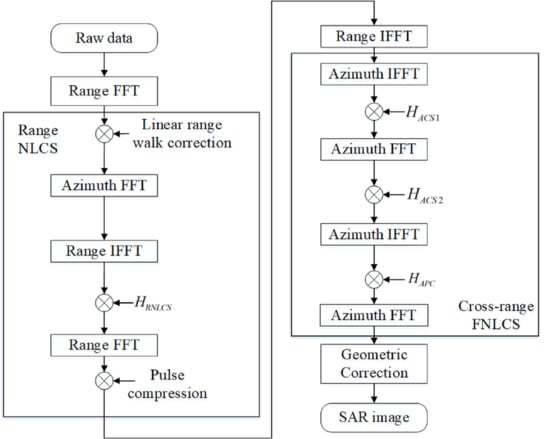
In this section, we will discuss the BFSAR echo model and the slant range model in the mini-UAV-based system, which is the basis of the following NLCS algorithm. The general imaging geometry of BFSAR is shown in Figure 1. The ENU (East, North, Up) coordinate system is adopted, where the x-axis represents the east, the y-axis represents the north and the z-axis represents up. The origin is the central position of the target area, where an arbitrary point scatterer uses the location vector $\mathbf{P}$. The transmitter has a velocity vector ${\mathbf{V}}_t$, and the receiver has a different velocity vector ${\mathbf{V}}_r$. The trajectory vector of the transmitter is ${\mathbf{R}}_t$ at $t_a=0$ and the corresponding trajectory vector of the receiver is ${\mathbf{R}}_r$. As mentioned in the previous section, the receiver flies forward towards the target area, and the transmitter illuminates the target area from a squint angle. The incident angle ${\theta }_{inR}$, ${\theta }_{inT}$ and squint angle ${\theta }_{sqT}$ shown in Figure 1 are measured at $t_a=0$. Under the interference of the external environment, the flight paths of the platforms cannot be expressed in a linear model, and the actual trajectories are shown with the blue lines.

In monostatic SAR systems, a forward-looking configuration cannot form an effective Doppler bandwidth, making it impossible to achieve a high resolution along the azimuth direction, and mirror effects would also happen in the scene. However, in BFSAR systems, the transmitter and receiver platforms are separated. In our system, the transmitter adopts a squinted configuration to achieve azimuth resolution, and the receiver adopts the forward-looking configuration to meet the system requirements.

Since the mini-UAV platform is lighter than the traditional SAR carrier, it is more susceptible to external interference; thus, the trajectory is more complicated. The traditional linear trajectory model cannot be used and needs to be extended for the mini-UAV platforms as follows:

$$\begin{array}{c}{\mathbf{R}}_t\left(t_a\right)={\mathbf{R}}_{t0}+{\mathbf{V}}_t{t}_a+\frac{1}{2}{\mathbf{a}}_t{t}_a^2+\frac{1}{6}{\mathbf{b}}_t{t}_a^3,\hfill \\ {\mathbf{R}}_r\left(t_a\right)={\mathbf{R}}_{r0}+{\mathbf{V}}_r{t}_a+\frac{1}{2}{\mathbf{a}}_r{t}_a^2+\frac{1}{6}{\mathbf{b}}_r{t}_a^3,\hfill \end{array}$$

(1)

where the slow time is $t_a$. $\mathbf{a}$ and $\mathbf{b}$ represent the acceleration vector and jerk vector, respectively. These vectors represent the components in the X, Y and Z directions. Taking ${\mathbf{R}}_{t0}$ (transmitter trajectory at $t_a=0$) as an example:

$${\mathbf{R}}_{t0}={\left[R_{t0x}{R}_{t0y}{R}_{t0z}\right]}^T.$$

(2)

By introducing the second- and third-order terms of the platform trajectory, the deviations in the actual experiment can be accurately described. In traditional SAR, the trajectory can be modeled in the linear expression of slow time, neglecting the acceleration and jerk of the platform. This is acceptable because the larger platform is more stable, but it is not suitable for systems with mini-UAV platforms, and so the nonlinear model in (1) is necessary. Based on the real data of the GPS and Inertial Navigation Systems (INS) for the mini-UAVs in the experiment with the parameters in

Table 1. SAR system parameters.

Parameter	Values
Radar wavelength	$0.02$ m
Sampling frequency	120 MHz
Range bandwidth	50 MHz
Signal pulse width	3 $\mathsf{\mu }$s
Chirp rate	$16.67$ MHz/$\mathsf{\mu }$s
Pulse repeat frequency	1200 Hz
Synthetic aperture time	$2.7$ s
Receiver slant range	3024 m
Receiver squint angle	${88}^{\circ }$
Receiver incident angle	${66}^{\circ }$
Receiver velocity	$19.31$ m/s
Receiver acceleration	$0.82$ m/s2
Receiver jerk	$0.23$ m/s3
Transmitter slant range	1905 m
Transmitter squint angle	47${}^{\circ }$
Transmitter incident angle	64${}^{\circ }$
Transmitter velocity	$21.12$ m/s
Transmitter acceleration	$1.14$ m/s2
Transmitter jerk	$0.30$ m/s3

, the accuracy of (1) is calculated as follows. Figure 2a,c show the trajectory errors of the traditional model of the transmitter and receiver, respectively. Figure 2b,d show the results of the extended model. The trajectory errors of the traditional model are much larger than the wavelength, but the errors of the extended model are smaller than $\lambda /8$ ($\lambda$ is the wavelength), which will not affect the image results.

Based on (1), when the target coordinate is $\mathbf{P}$, the slant range can be expressed as

$$\begin{array}{c}R\left(t_a\right)=\left|{\mathbf{R}}_t\left(t_a\right)-\mathbf{P}\right|+\left|{\mathbf{R}}_r\left(t_a\right)-\mathbf{P}\right|\hfill \\ =\left|{\mathbf{R}}_{t0}+{\mathbf{V}}_t{t}_a+\frac{1}{2}{\mathbf{a}}_t{t}_a^2+\frac{1}{6}{\mathbf{b}}_t{t}_a^3-\mathbf{P}\right|+\left|{\mathbf{R}}_{r0}+{\mathbf{V}}_r{t}_a+\frac{1}{2}{\mathbf{a}}_r{t}_a^2+\frac{1}{6}{\mathbf{b}}_r{t}_a^3-\mathbf{P}\right|.\hfill \end{array}$$

(3)

Assuming a linear FM pulse is emitted by the transmitter, the echo from target $\mathbf{P}$ can be expressed as

$$\begin{array}{c}s{s}_1\left(t_r,t_a\right)=rect\left[\frac{t_r-R\left(t_a\right)/c}{T_p}\right]exp\left(j\pi K_b{\left(t_r-\frac{R\left(t_a\right)}{c}\right)}^2\right)\times rect\left(\frac{t_a}{T_{int}}\right)exp\left(-j\frac{2\pi R\left(t_a\right)}{\lambda }\right)\hfill \end{array}.$$

(4)

where $t_r$ is the fast time, c is the light speed, $T_p$ is the pulse width, $K_b$ is the FM rate and $T_{\mathrm{int}}$ is the synthetic aperture time.

As mentioned before, (3) gives the accurate bistatic slant range model, but it is not suitable for the derivation of the NLCS algorithm. Thus, (3) needs to be further analyzed in a sufficiently simple form without loss of accuracy. Therefore, the third-order Taylor expansion performed on the slant range model (3) at $t_a=0$ is expressed as

$$R\left(t_a\right)=R_e+V_e{t}_a+\frac{1}{2}{a}_e{t}_a^2+\frac{1}{6}{b}_e{t}_a^3.$$

(5)

The coefficients of (5) are shown in (6).

$$\begin{array}{c}{R}_e=\left|{\mathbf{R}}_{r0}-\mathbf{P}\right|+\left|{\mathbf{R}}_{t0}-\mathbf{P}\right|V_e=\frac{{\left({\mathbf{R}}_{r0}-\mathbf{P}\right)}^T{\mathbf{V}}_r}{\left|{\mathbf{R}}_{r0}-\mathbf{P}\right|}+\frac{{\left({\mathbf{R}}_{t0}-\mathbf{P}\right)}^T{\mathbf{V}}_t}{\left|{\mathbf{R}}_{t0}-\mathbf{P}\right|}\hfill \\ a_e=-\frac{{\left({\left({\mathbf{R}}_{r0}-\mathbf{P}\right)}^T{\mathbf{V}}_r\right)}^2}{2{\left|{\mathbf{R}}_{r0}-\mathbf{P}\right|}^3}+\frac{\left[{\left({\mathbf{R}}_{r0}-\mathbf{P}\right)}^T{\mathbf{a}}_r+{\left|{\mathbf{V}}_r\right|}^2\right]}{\left|{\mathbf{R}}_{r0}-\mathbf{P}\right|}-\frac{{\left({\left({\mathbf{R}}_{t0}-\mathbf{P}\right)}^T{\mathbf{V}}_t\right)}^2}{2{\left|{\mathbf{R}}_{t0}-\mathbf{P}\right|}^3}+\frac{\left[{\left({\mathbf{R}}_{t0}-\mathbf{P}\right)}^T{\mathbf{a}}_t+{\left|{\mathbf{V}}_t\right|}^2\right]}{\left|{\mathbf{R}}_{t0}-\mathbf{P}\right|}\hfill \\ b_e=\frac{3{\left({\left({\mathbf{R}}_{r0}-\mathbf{P}\right)}^T{\mathbf{V}}_r\right)}^3}{4{\left|{\mathbf{R}}_{r0}-\mathbf{P}\right|}^5}-\frac{3{\left({\mathbf{R}}_{r0}-\mathbf{P}\right)}^T{\mathbf{V}}_r\left[{\left({\mathbf{R}}_{r0}-\mathbf{P}\right)}^T{\mathbf{a}}_r+{\left|{\mathbf{V}}_r\right|}^2\right]}{{\left|{\mathbf{R}}_{r0}-\mathbf{P}\right|}^3}+\frac{{\left({\mathbf{R}}_{r0}-\mathbf{P}\right)}^T{\mathbf{b}}_r+3{{\mathbf{V}}_r}^T{\mathbf{a}}_r}{\left|{\mathbf{R}}_{r0}-\mathbf{P}\right|}\hfill \\ +\frac{3{\left({\left({\mathbf{R}}_{t0}-\mathbf{P}\right)}^T{\mathbf{V}}_t\right)}^3}{4{\left|{\mathbf{R}}_{t0}-\mathbf{P}\right|}^5}-\frac{3{\left({\mathbf{R}}_{t0}-\mathbf{P}\right)}^T{\mathbf{V}}_t\left[{\left({\mathbf{R}}_{t0}-\mathbf{P}\right)}^T{\mathbf{a}}_t+{\left|{\mathbf{V}}_t\right|}^2\right]}{{\left|{\mathbf{R}}_{t0}-\mathbf{P}\right|}^3}+\frac{{\left({\mathbf{R}}_{t0}-\mathbf{P}\right)}^T{\mathbf{b}}_t+3{{\mathbf{V}}_t}^T{\mathbf{a}}_t}{\left|{\mathbf{R}}_{t0}-\mathbf{P}\right|}\hfill \end{array}$$

(6)

It can be seen from (6) that both acceleration vectors and jerk vectors of the transmitter and receiver are considered and play a vital role in the slant range model to ensure its accuracy for the mini-UAV-based system. Based on the real experimental data in Table 1, the accuracy of the bistatic slant range model in (5) is calculated as shown in Figure 3. We simulate for four point-scatterers. Target 1, 2, 3, 4 respectively correspond to the point scatterer at the coordinate $\left(500,500\right)$, $\left(-500,500\right)$, $\left(500,-500\right)$ and $\left(-500,-500\right)$, and each curve represents the error of a target point under a slant range expression. Compared with the traditional slant range model shown in Figure 3a, the new model can reflect the inherited trajectory deviations of mini-UAV platforms, as shown in Figure 3b. For a Ku-band system, the errors are smaller than $\lambda /8$, which indicates that the new slant range model can be used under this condition.

3. NLCS Algorithm

An improved frequency-domain algorithm is proposed for mini-UAV-based BFSAR, and the flowchart of the algorithm is shown in Figure 4. First, a new range NLCS operator was derived based on the accurate bistatic slant range model in (5). Second, based on (5), a new azimuth NLCS operator in the Doppler frequency domain was established regarding the spotlight illumination of the transmitter and receiver in the mini-UAV-based system. The simulation and numerical results are all based on the real data sets in Table 1 of a mini-UAV-based BFSAR data acquisition campaign on July 2018.

3.1. Range Processing Using NLCS

Since the new slant range model has taken the UAVs’ acceleration and jerk vectors into consideration, the high-order phase and the RCM spatial variance model need to be extended for mini-UAV-based BFSAR system.

According to [34,48], linear range walk correction is performed to prevent the signal from aliasing in the Doppler domain. The signal after linear range walk correction is

$$\begin{array}{c}S{s}_2\left(f,t_a\right)=rect\left(\frac{f}{K_b{T}_p}\right)exp\left(-j\pi \frac{f^2}{K_b}\right)rect\left(\frac{t_a}{T_{\mathrm{int}}}\right)\times \hfill \\ exp\left[-j\frac{2\pi \left(f_c+f\right)}{c}\left(R_e+V_{sv}{t}_a+\frac{1}{2}{a}_e{t}_a^2+\frac{1}{6}{b}_e{t}_a^3\right)\right].\hfill \end{array}$$

(7)

where $f_c$ is the carrier frequency, $V_{sv}=V_e-V_{ref}$ is the velocity residual and $V_{ref}$ is the reference velocity at the target area central. Based on the series reversion [35] principle, the above signal could be transformed into the 2D frequency domain, and we obtain

$$\begin{array}{c}S{S}_3\left(f,f_d\right)=\mathrm{rect}\left(\frac{f}{K_b{T}_p}\right)exp\left(-j\pi \frac{f^2}{K_m}-j2\pi \left(\frac{R_e+RCM}{c}\right)f\right)\times \mathrm{rect}\left(\frac{f_d+V_{sv}/\lambda }{a_e/\lambda ·T_{\mathrm{int}}}\right)\hfill \\ exp\left(j\pi \lambda \left(\frac{1}{a_e}+\frac{b_e{V}_{sv}}{a_e^3}\right)f_d^2+j2\pi \left(\frac{V_{sv}}{a_e}+\frac{b_e{V}_{sv}^2}{2a_e^3}\right)f_d+j\pi \frac{{\lambda }^2{b}_e}{3a_e^3}{f}_d^3-j2\pi \frac{R_e}{\lambda }+j\pi \frac{V_{sv}^2}{\lambda a_e}\left(1+\frac{b_e{V}_{sv}}{3a_e^2}\right)\right),\hfill \end{array}$$

(8)

where

$$\left\{\begin{array}{c}RCM=\frac{{\lambda }^2}{2}\left(\frac{1}{a_e}+\frac{b_e{V}_{sv}}{{a_e}^3}\right){f_d}^2+\frac{{\lambda }^3{b}_e{f_d}^3}{3{a_e}^3}-\frac{{V_{sv}}^2}{2a_e}\left(1+\frac{b_e{V}_{sv}}{3{a_e}^2}\right)\hfill \\ K_m={\left(\frac{1}{K_b}-\frac{\lambda }{a_e}\frac{{f_d}^2}{{f_c}^2}-\frac{{\lambda }^2{b}_e{f_d}^3}{{a_e}^3{f_c}^2}\right)}^{-1}\hfill \end{array}\right.$$

(9)

by introducing new variables as

$$\begin{array}{c}{\varphi }_{a0}=-2\pi \frac{R_e}{\lambda }+\pi \frac{{V_{sv}}^2}{\lambda a_e}\left(1+\frac{b_e{V}_{sv}}{3{a_e}^2}\right),\hfill \\ K_r=-\frac{{a_e}^3}{\lambda \left({a_e}^2+b_e{V}_{sv}\right)},\hfill \\ t_{ap}=-\left(\frac{V_{sv}}{a_e}+\frac{b_e{V_{sv}}^2}{2{a_e}^3}\right),\hfill \end{array}$$

(10)

we obtain

$$\begin{array}{c}S{S}_4\left(f,f_d\right)=rect\left(\frac{f}{K_b{T}_p}\right)exp\left(-j\pi \frac{f^2}{K_m}-j2\pi \left(\frac{R_e+RCM}{c}\right)f\right)\times \hfill \\ rect\left(\frac{f_d+V_{sv}/\lambda }{a_e/\lambda ·T_{\mathrm{int}}}\right)exp\left(-j\pi \frac{f_d^2}{K_r}-j2\pi f_d{t}_{ap}+j\pi \frac{{\lambda }^2{b}_e}{3a_e^3}{f}_d^3+j{\varphi }_{a0}\right).\hfill \end{array}$$

(11)

In the first exponential expression in (11), the first phase term is for the range quadrature phase and the second one is for range cell migration. In the second exponential expression in (11), the first phase term is for the azimuth quadrature phase, the second term is for the azimuth coordinate of the point target, the third term is for the azimuth cubic phase and the fourth term is for the constant azimuth phase.

For range cell migration in (11), we obtain

$$RCM\left(f_d\right)=\frac{{\lambda }^2}{2}\left(\frac{1}{a_e}+\frac{b_e{V}_{sv}}{a_e^3}\right)f_d^2+\frac{{\lambda }^3{b}_e{f}_d^3}{3a_e^3}-\frac{V_{sv}^2}{2a_e}\left(1+\frac{b_e{V}_{sv}}{3a_e^2}\right)\approx 0.$$

(12)

It is clear from (12) that $\left(R_e,t_{ap}\right)$ defines the coordinate of the point target in the bistatic slant plane. Furthermore, a mapping operator between $\left(R_e,t_{ap}\right)$ and $\left(X,Y\right)$ could be established in (6) and (10), which are also be used for geometric correction.

Then, transforming the signal into the range-Doppler domain, we obtain

$$\begin{array}{c}s{S}_5\left(t_r,f_d\right)=\mathrm{rect}\left(\frac{V_{sv}+\lambda f_d}{a_e{T}_{\mathrm{int}}}\right)\mathrm{rect}\left(\frac{t_r-\left(R_e+RCM\left(f_d\right)\right)/c}{B/K_m}\right)\times exp\left(j\pi K_m{\left(t_r-\frac{R_e+RCM\left(f_d\right)}{c}\right)}^2\right)\hfill \\ exp\left(-j\pi \frac{f_d^2}{K_r}-j2\pi f_d{t}_{ap}+j\pi \frac{{\lambda }^2{b}_e}{3a_e^3}{f}_d^3+j{\varphi }_{a0}\right).\hfill \end{array}$$

(13)

Inspecting (9) and (13), the expression is shown to be more accurate than that in the monostatic case because the term $b_e$ is introduced here.

As mentioned before, the spatial variance of RCM in the mini-UAV-based BFSAR system is much worse than in the traditional approach. Therefore, a new RCM spatial variance model needs to be re-derived as follows:

$$RCM\left(f_d;R_e,t_{ap}\right)=RCM\left(f_d;R_{eref},t_{apref}\right)+\frac{\partial RCM}{\partial R_e}\left(R_e-R_{eref}\right)+\frac{{\partial }^{2}RCM}{2\partial R_e^2}{\left(R_e-R_{eref}\right)}^2,$$

(14)

where $ref$ stands for reference. The partial derivatives in the former equation are too complex to obtain the analytical formulas, and thus we turn to the numerical solution of (12) and (14). Note that the RCM spatial variance is along the slant range and is a curve in the X–Y coordinates, which is different from the case in the monostatic SAR system.

Under real mini-UAV-based BFSAR parameters, the range RCM error (RCME) of targets 13 and 23 are calculated. Targets are defined in Figure 5 and the reference target is target 3. The range resolution of the system is around 3 m. The results of the residual RCM with the traditional NLCS model [41] are shown in Figure 6a. It can be clearly seen that the RCME is larger than the half range resolution cell and has severe impacts on imaging. The RCME of each target with the proposed model is shown in Figure 6b. The residual RCM is smaller than the half range resolution cell, which will not affect the imaging results.

After the variance model is established, the CS operator is introduced as

$$\begin{array}{c}{H}_{RNLCS}\left(t_r,f_d\right)=exp\left(-j\pi K_m{C}_2\left(f_d\right){\left(t_r-\frac{R_{eref}+RCM\left(f_d;R_{eref},t_{apref}\right)}{c}\right)}^2\right)\hfill \\ \times exp\left(-j\pi K_m{C}_3\left(f_d\right){\left(t_r-\frac{R_{eref}+RCM\left(f_d;R_{eref},t_{apref}\right)}{c}\right)}^3\right).\hfill \end{array}$$

(15)

The CS operator can be calculated as

$$\left\{\begin{array}{c}{C}_2\left(f_d\right)=-\frac{\partial RCM}{\partial R_e}\hfill \\ C_3\left(f_d\right)=-\frac{c}{3}\frac{{\partial }^{2}RCM}{\partial R_e^2}\hfill \end{array}\right.$$

(16)

Then, residual phase compensation and pulse compression need to be performed; the signal after NLCS processing is

$$\begin{array}{c}S{S}_6\left(f,f_d\right)=\mathrm{rect}\left(\frac{f}{B}\right)exp\left[j{\mathrm{\Theta }}_0\left(f_d;R_e\right)\right]exp\left(-j\frac{\pi f^2}{K_m\left(1+\frac{\partial RCM}{\partial R_e}\right)}-j2\pi f\frac{R_e+RCM\left(f_d;R_{eref},t_{apref}\right)}{c}\right)\hfill \\ \times \mathrm{rect}\left(\frac{V_{sv}+\lambda f_d}{a_e{T}_{\mathrm{int}}}\right)exp\left(-j\pi \frac{f_d^2}{K_r}-j2\pi f_d{t}_{ap}+j\pi \frac{{\lambda }^2{b}_e}{3a_e^3}{f}_d^3+j{\varphi }_{a0}\right),\hfill \end{array}$$

(17)

where

$${\mathrm{\Theta }}_0=\pi K_m\frac{{\left(R_e-R_{eref}\right)}^2}{c^2}\left\{\begin{array}{c}{\left(\frac{\partial RCM}{\partial R_e}+\frac{{\partial }^{2}RCM}{2\partial {R_e}^2}(R_e-R_{eref})\right)}^2+\frac{\partial RCM}{\partial R_e}+\frac{1}{3}\frac{{\partial }^{2}RCM}{\partial {R_e}^2}\left(R_e-R_{eref}\right)\hfill \end{array}\right\}.$$

(18)

Inspecting (17), the RCM of different positions has been corrected to the reference position. The RCM of the reference position can be used to compensate all the images. By compensating ${\mathrm{\Theta }}_0$ and performing range compression and secondary range compression and transforming the signal into fast time domain, we have

$$s{S}_7\left(t_r,f_d\right)=\mathrm{sinc}\left(B\left(t_r-\frac{R_e}{c}\right)\right)\times \mathrm{rect}\left(\frac{V_{sv}+\lambda f_d}{a_e{T}_{\mathrm{int}}}\right)exp\left(-j\pi \frac{f_d^2}{K_r}-j2\pi f_d{t}_{ap}+j\pi \frac{{\lambda }^2{b}_e}{3a_e^3}{f}_d^3+j{\varphi }_{a0}\right).$$

(19)

Thus far, the spatial variance of RCM along the range direction has been compensated, and the pulse compression has also been completed. The cross-range processing will be carried out in the next subsection.

3.2. Cross-Range Processing Using FNLCS

In order to account for the spotlight mode of the system, the cross-range nonlinear CS operator based on the new slant range model is derived in the Doppler frequency domain, and the proposed compensation operator of the variant phase is shown to be more accurate than the traditional one.

According to (19), the cross-range signal in the time domain can be rewritten as

$$s_{a1}\left(t_a,R_e\right)=\omega \left(t_a\right)\times exp\left(\begin{array}{c}j{\varphi }_{a0}+j\pi K_r{\left(t_a-t_{ap}\right)}^2+j\pi K_t{\left(t_a-t_{ap}\right)}^3\hfill \end{array}\right),$$

(20)

where the coefficient of cubic-term $K_t$ is

$$K_t=-\frac{\left({a_e}^6{b}_e\right)}{3\left(\lambda {\left({a_e}^2+b_e{V}_{sv}\right)}^3\right)}.$$

(21)

It can be seen from Section 3 that the dependence of $K_r$ and $K_t$ on the $R_e$ could be compensated by means of the dynamic focusing method. However, the dependence on $t_{ap}$ and the cross-range variance could not be compensated since the signal shared the same Doppler time domain. To deal with the cross-range variance, the parameters $K_r$ and $K_t$ should firstly be modeled as the functions of the variable $t_{ap}$; then, we obtain

$$\begin{array}{c}{K}_r(t_{ap};R_e)=K_r\left(t_{apref};R_e\right)+\frac{\partial K_r}{\partial t_{ap}}\left(t_{ap}-t_{apref}\right)+\frac{{\partial }^2{K}_r}{2\partial t_{ap}^2}{\left(t_{ap}-t_{apref}\right)}^2,\hfill \\ K_t(t_{ap};R_e)=K_t\left(t_{apref};R_e\right)+\frac{\partial K_t}{\partial t_{ap}}\left(t_{ap}-t_{apref}\right),\hfill \end{array}$$

(22)

where $ref$ is the reference point. Note that the above model should be determined in the specific range bin $R_e$. The diagram is shown in Figure 7. $P_1$ and $P_2$ have the same slant range of $R_e$; after the range processing, their pulse pressure results are corrected to the same range bin. However, there is still spatial variance along the cross-range direction; thus, (22) establishes the model between $K_r$ and $t_{ap}$ and the model between $K_t$ and $t_{ap}$ to solve this problem under the mini-UAV-based BFSAR condition.

Under real mini-UAV-based BFSAR parameters, based on the above analysis, the calculation results of $K_r$ and $K_t$ are shown in Figure 8. Figure 8a is calculation results of $K_r$, where the blue line is the error of the traditional NLCS model, the phase error is greater than $\lambda /4$, and the red line is the modeling algorithm proposed in this paper, the phase error of which is smaller than $\lambda /4$ and will not affect the imaging results. Similarly, Figure 8b is the calculation results for $K_t$. Compared with the traditional model, the error introduced by the proposed model is much smaller.

Based on the former analysis, FNLCS processing in the Doppler frequency domain is proposed to account for the compensation of the cross-range variance. Inspecting (20), the variant higher phase term needs first to be corrected by

$$H_{ACS1}\left(t_a\right)=exp\left(j\pi p{t}_a^3+j\pi q{t}_a^4\right),$$

(23)

where p and q are the variables to be determined in the following sections.

Combining (20) and (23) and transforming the result into the Doppler frequency domain,

$$\begin{array}{c}{S}_{a2}\left(f_d,R_e\right)=\omega \left(f_d\right)\hfill \\ exp\left(j{\varphi }_{a0}-j2\pi f_d{t}_{ap}-j\pi \frac{f_d^2}{K_r}+j\pi K_t{\left(\frac{f_d}{K_r}\right)}^3+j\pi p{\left(\frac{f_d}{K_r}+t_{ap}\right)}^3+j\pi q{\left(\frac{f_d}{K_r}+t_{ap}\right)}^4\right).\hfill \end{array}$$

(24)

According to the analysis above, the variance along the cross-range direction is compensated through the operator as

$$H_{ACS2}\left(f_d\right)=exp\left(j\pi s_2{f}_d^2+j\pi s_3{f}_d^3+j\pi s_4{f}_d^4\right),$$

(25)

where $s_2$, $s_3$ and $s_4$ are also variables based on the BiSAR configuration. Multiplying (24) and (25), we obtain

$$\begin{array}{c}{S}_{a3}\left(f_d,R_e\right)=\omega \left(f_d\right)exp\left(j{\varphi }_{a0}-j2\pi f_d{t}_{ap}-j\pi \frac{f_d^2}{K_r}+j\pi s_2{f}_d^2+j\pi K_t{\left(\frac{f_d}{K_r}\right)}^3+j\pi s_3{f}_d^3+j\pi s_4{f}_d^4\right)\hfill \\ exp\left(j\pi p{\left(\frac{f_d}{K_r}+t_{ap}\right)}^3+j\pi q{\left(\frac{f_d}{K_r}+t_{ap}\right)}^4\right),\hfill \end{array}$$

(26)

and then transforming (26) into the slow time domain, the derivation is shown in Appendix A. Based on the cross-range spatial variance model in (22), the expression of $s_2$, $s_3$, $s_4$, p and q can be calculated. The final signal expression in the slow time domain is

$$S_{a4}\left(t_a\right)=w\left(t_a\right)exp\left(-j\frac{\pi K_{rref}}{\alpha }{t}_{ap}{t}_a\right)exp\left(jA\right).$$

(27)

Under the mini-UAV-based BFSAR system, the compensation factor has a large bandwidth, which could exceed the $PRF$ or $T_{int}$ limit. Thus, it is necessary to check whether the compensation operator is aliased. If this occurs, $PRF$ or $T_{int}$ can be increased by adding zeros.

Inspecting (27), it is evident that the cross-range-dependent modulation terms and the cross-range-dependent geometric shift are all removed. Next, it is only required to multiply the conjugate of A. The operator is expressed as

$$H_{APC}=exp\left(-jA\right).$$

(28)

Multiplying (27) with (28) and transforming the result into the Doppler frequency domain, the final focused SAR image is obtained as

$$\begin{array}{c}s{S}_8(t_r,f_d)=sinc\left(B(t_r-\frac{R_e}{c})\right)·sinc\left(T_{\mathrm{int}}(f_d-\frac{t_{ap}{K}_{rref}}{2\alpha })\right)exp\left(j{\varphi }_{a0}\right).\hfill \end{array}$$

(29)

Inspecting (29), it can be found that the target is focused at the position $\left(R_e/c,t_{ap}{K}_{rref}/2\alpha \right)$, which has an offset in the cross-range direction. To solve this problem, the cross-range sampling interval $\mathsf{\Delta }x$ can be adjusted by multiplying by $2\alpha$ to put the target into the correct position.

For the traditional time NLCS algorithm [34,49], in the stripmap mode, the support zones of different targets in one range cell are separated. An operator is applied in the time domain to correct the phases of different targets so that the cross-range variance is compensated.

However, when the SAR system adopts the spotlight mode, as shown in Figure 9a, the support zones of different targets become the same because the beam center always points to the target area. The phase correction of the slow time domain operator is the same for each target point. Therefore, the variance along the cross-range direction cannot be compensated in the time domain.

In contrast, when the spotlight mode is adopted, as shown in Figure 9b, the support zones of different target points are separated in the Doppler frequency domain, meaning that NLCS can be used in this domain. Therefore, a frequency NLCS algorithm is proposed to compensate the variance along the cross-range direction.

4. Simulations

To verify the feasibility and effectiveness of the proposed algorithm, a simulation was performed. The parameters are shown in Table 1. The simulation was implemented on an array of 25 targets located in a 1.6 km × 1.6 km area on the ground plane, as shown in Figure 5. Each target was 400 m away from the adjacent target both in the x-axis and y-axis directions.

First, the errors of different slant range models in the mini-UAV-based BFSAR system were simulated. According to the data recorded by GPS and INS, the true slant range value at each moment could be obtained. The error under different slant range models could be calculated as shown in Figure 3. It can be seen that the traditional linear model was not sufficient to describe the movement of the mini-UAV, as the error was much larger than the wavelength, while the proposed extended slant range model could describe the movement of the mini-UAV well, and the slant range error was smaller than $\lambda /8$.

Then, the range direction RCM variance compensation results were simulated. In the forward-looking configuration, Figure 10 shows the simulation results of target points 1 and 25. After range NLCS, the signal in the cross-range frequency domain is shown. Figure 10a shows the simulation result of the traditional range NLCS [41]. Because the slant range variant model cannot used in the bistatic configuration, the side lobes of the image results after the range NLCS were asymmetric and not well focused. Figure 10b shows the range NLCS result of the algorithm proposed in this paper. For the points 1 and 25 with the largest variance in the scene, the algorithm could focus well, and the side lobe level was close to the theoretical value.

After range pulse compression, under the mini-UAV-based BFSAR condition, the addition of zeros is required to prevent aliasing. The simulation results are shown in Figure 11. Figure 11a is the result without adding zeros. It is evident that there is a false target in the cross-range direction. Figure 11b is the result after adding zeros. It is obvious that the focusing result is ideal, and PeakSidelobe Ratio (PSLR) and Integrated Sidelobe Ratio (ISLR) are close to the theoretical value.

Next, two algorithms were applied to process the simulated data. No weighting function or sidelobe control approach was used during the image simulation. The effect of factor $\alpha$ was eliminated so that the imaging results of the three algorithms could be presented under the same metric, which was convenient for the comparison of results. Figure 12 shows the imaging results of the targets 1, 5, 21 and 25 using the two algorithms. All of the extracted subimages were interpolated by zero padding to increase the fineness of the image. Figure 12a shows the imaging results of the traditional NLCS algorithm [41]; the variance along the range and cross-range direction is considered. However, the traditional monostatic variance modeling method introduces large errors under the mini-UAV-based BFSAR system, meaning that the variance in the image scene cannot be fully compensated. At the same time, the system’s slant range expression is not sufficiently accurate, which means that all targets are defocused. Figure 12b shows the imaging results of the proposed algorithm. In the imaging process, the factor $\alpha$ was set to 0.55 and the result corrected the effect of $\alpha$. It can be seen that all of the targets are well focused.

Figure 13 shows the imaging results of target 1 and target 25 along two directions. In order to facilitate the comparison, the cross-range cell intervals in the slow time domain and the Doppler frequency domain have been corrected for consistency. As shown in Figure 13a,b, in the range direction for the traditional NLCS algorithm, due to the residual RCM error, the first side lobe is slightly higher than the theoretical value. The proposed algorithm has fewer residual RCM errors and the first side lobe is close to the theoretical value. Figure 13c,d show the results in the cross-range direction. The variance model along this direction in the proposed algorithm is more effective than the model in traditional algorithm. Thus, the variance of the $K_r$ and $K_t$ could be compensated well. The high-order phase in the cross-range direction could also be compensated to a low level, with PSLR and ISLR almost equal to the theoretical value. In order to better compare the imaging results of the two algorithms, the resolution, PSLR and ISLR of the four targets are shown in

Table 2. Measured parameters of the selected targets.

		Target 1	Target 5	Target 21	Target 25
Traditional NLCS algorithm [41]
Resolution (m)	Range	3.75	3.75	3.70	3.77
	Cross-range	1.46	1.48	1.51	1.54
PSLR (dB)	Range	−10.86	−11.1	−10.12	−10.89
	Cross-range	−9.73	−9.82	−10.73	−7.22
ISLR (dB)	Range	−10.12	−10.82	−9.63	−9.32
	Cross-range	−9.32	−8.88	9.96	−6.52
Proposed algorithm
Resolution (m)	Range	3.75	3.73	3.70	3.72
	Cross-range	1.42	1.46	1.44	1.44
PSLR (dB)	Range	−13.31	−13.01	−12.84	−12.54
	Cross-range	−12.7	−12.62	−13	−12.64
ISLR (dB)	Range	−11.33	−11.02	−11.42	−11.56
	Cross-range	−10.87	−10.37	−11.24	−11.42

.

5. Processing Results of Real Data

This experiment is based on a mini-UAV-SAR system in the Ku-band. The transmitter and receiver are mounted on two mini-UAVs, respectively. The experimental site was selected on the outskirts of Baotou City, and the parameters are the same as Table 1. The experimental scenario consisted of several rows of neat rooms and two transponders. The BFSAR data were acquired on July 2018.

In this experiment, both the transmitter and receiver adopted small 1 kg SAR systems. Because the system was light, the selected mini-UAVs were also light, meaning the system was vulnerable to interference from the external environment. At the same time, because the experimental site was selected in the suburbs, the wind was relatively strong, which meant that the mini-UAV carrier itself shook seriously, resulting in higher system acceleration and jerk compared to large aircraft.

Utilizing the direct signal, time and phase synchronization errors were compensated. The algorithm in [41] was used to process the echo data, and the imaging result after radiometric and geometric corrections is shown in Figure 14a. As seen and analyzed, when the traditional algorithm was used, the boundary of the room was blurred, and both transponders experienced defocusing.

The proposed imaging algorithm in this paper was also applied to focus the synchronized echo data, and the result is shown in Figure 14b. The result was also corrected to the ground plane. With the algorithm proposed in this paper, the boundary of the room area was clearer, and the transponders were well focused.

Figure 15 shows the contour of the left transponder. Since the back scattering coefficient of the surrounding area was low, the surrounding area had less influence on the image result of the transponder, meaning that the image result could reflect the focusing effects more accurately. Figure 15a is the result of the algorithm proposed in [41], where the cross-range direction was poorly focused. Figure 15b is the result of the proposed algorithm, where the target was well focused along two dimensions.

6. Discussion

The feasibility of the proposed algorithm is verified by simulation and real data. According to the actual UAV-based system conditions we demonstrate the compensation effect of the proposed algorithm for the spatial variance, according to the actual UAV-based system conditions by simulations for a scatterers array. We compare the focus effect of the traditional and proposed algorithm. It’s found that the traditional algorithm cannot obtain well-focused images under the conditions of UAV-based BFSAR system, which is because that the accuracy of the spatial variance model cannot meet the requirements of the system, so the PSLR and ISLR increase. The proposed algorithm takes into account the higher order of the slant range and spatial variance model, and performs more accurate compensation. Therefore, the proposed algorithm can obtain better-focused image, and is more suitable for the UAV-based BFSAR systems.

The effectiveness of the proposed algorithm is also verified by real data. There is a plant in the experimental scene, and two transponders are placed diagonally across the plant. The well-focused image proves that the spatial variance is well compensated, and the accuracy of the slant range model meets the requirements of the UAV system. The focus effect of the transponder clearly demonstrates the focusing performance of the algorithm, which is greatly improved compared with traditional algorithms. In short, this paper verifies the applicability of the proposed algorithm. However, in the case of insufficient positioning accuracy of the platform, a motion compensation algorithm is needed to further improve the image quality.

7. Conclusions

This paper presents an improved image formation algorithm suitable for mini-UAV-based BFSAR systems. Based on the system configuration and the mini-UAVs’ motion characteristics, acceleration and jerk are introduced in the slant range model. Considering the difference between the monostatic and bistatic SAR system, the variance model for mini-UAV-based BFSAR is established. At the same time, a frequency-domain imaging algorithm is proposed for the spotlight mode. The results of the simulation and the image obtained using real bistatic SAR data validate the feasibility and effectiveness of the algorithm.

References

1. Cumming, I.G.; Wong, F.H. The Digital Processing of Seasat Synthetic Aperture Radar Data; Artech House: Norwood, MA, USA, 2005. [Google Scholar]
2. Quegan, S. Spotlight synthetic aperture radar: Signal processing algorithms. J. Atmos. Sol.-Terr. Phys. 1997, 59, 597–598. [Google Scholar] [CrossRef]
3. Qiu, X.; Hu, D.; Ding, C. Some Reflections on Bistatic SAR of Forward-Looking Configuration. IEEE Geosci. Remote Sens. Lett. 2008, 5, 735–739. [Google Scholar] [CrossRef]
4. Neo, Y.L.; Wong, F.; Cumming, I.G. A Two-Dimensional Spectrum for Bistatic SAR Processing Using Series Reversion. IEEE Geosci. Remote Sens. Lett. 2007, 4, 93–96. [Google Scholar] [CrossRef]
5. Yin, W.; Ding, Z.; Lu, X.; Zhu, Y. Beam scan mode analysis and design for geosynchronous SAR. Sci. China Inf. Sci. 2017, 60, 060306. [Google Scholar] [CrossRef]
6. Walterscheid, I.; Ender, J.; Brenner, A.; Loffeld, O. Bistatic SAR Processing and Experiments. IEEE Trans. Geosci. Remote Sens. 2006, 44, 2710–2717. [Google Scholar] [CrossRef]
7. Zheng, W.; Hu, J.; Zhang, W.; Yang, C.; Li, Z.; Zhu, J. Potential of geosynchronous SAR interferometric measurements in estimating three-dimensional surface displacements. Sci. China 2017, 60, 060304. [Google Scholar] [CrossRef]
8. Long, T.; Liang, Z.; Liu, Q. Advanced technology of high-resolution radar: Target detection, tracking, imaging, and recognition. Sci. China Inf. Sci. 2019, 62, 40301. [Google Scholar] [CrossRef] [Green Version]
9. Chang, S.; Zhang, H.; Long, T.; Liu, Q.; Zheng, L. A radar waveform bandwidth selection strategy for wideband tracking. Science China Inf. Sci. 2019, 62, 40306. [Google Scholar] [CrossRef] [Green Version]
10. Yuan, Y.; Cheng, L.; Wang, Z.; Sun, C. Position tracking and attitude control for quadrotors via active disturbance rejection control method. Sci. China Inf. Sci. 2018, 62. [Google Scholar] [CrossRef]
11. Heidarpour Shahrezaei, I.; Kazerooni, M.; Fallah, M. A complex target terrain SAR raw data generation and evaluation based on inversed equalized hybrid-domain algorithm processing. Waves Random Complex Media 2017, 27, 47–66. [Google Scholar] [CrossRef]
12. Zhang, Y.; Mao, D.; Zhang, Q.; Zhang, Y.; Huang, Y.; Yang, J. Airborne Forward-Looking Radar Super-Resolution Imaging Using Iterative Adaptive Approach. IEEE J. Sel. Top. Appl. Earth Obs. Remote Sens. 2019, 12, 2044–2054. [Google Scholar] [CrossRef]
13. Liang, Y.; Li, G.; Wen, J.; Zhang, G.; Dang, Y.; Xing, M. A Fast Time-Domain SAR Imaging and Corresponding Autofocus Method Based on Hybrid Coordinate System. IEEE Trans. Geosci. Remote Sens. 2019, 57, 8627–8640. [Google Scholar] [CrossRef]
14. Rodriguez-Cassola, M.; Prats, P.; Krieger, G.; Moreira, A. Efficient Time-Domain Image Formation with Precise Topography Accommodation for General Bistatic SAR Configurations. IEEE Trans. Aerosp. Electron. Syst. 2011, 47, 2949–2966. [Google Scholar] [CrossRef] [Green Version]
15. Ran, L.; Liu, Z.; Li, T.; Xie, R.; Zhang, L. An Adaptive Fast Factorized Back-Projection Algorithm With Integrated Target Detection Technique for High-Resolution and High-Squint Spotlight SAR Imagery. IEEE J. Sel. Top. Appl. Earth Obs. Remote Sens. 2018, 11, 171–183. [Google Scholar] [CrossRef]
16. Zhong, H.; Zhang, Y.; Chang, Y.; Liu, E.; Tang, X.; Zhang, J. Focus High-Resolution Highly Squint SAR Data Using Azimuth-Variant Residual RCMC and Extended Nonlinear Chirp Scaling Based on a New Circle Model. IEEE Geosci. Remote Sens. Lett. 2018, 15, 547–551. [Google Scholar] [CrossRef]
17. Wang, Y.; Li, J.; Xu, F.; Yang, J. A New Nonlinear Chirp Scaling Algorithm for High-Squint High-Resolution SAR Imaging. IEEE Geosci. Remote Sens. Lett. 2017, 14, 2225–2229. [Google Scholar] [CrossRef]
18. Liao, Y.; Liu, Q.H. Modified Chirp Scaling Algorithm for Circular Trace Scanning Synthetic Aperture Radar. IEEE Trans. Geosci. Remote Sens. 2017, 55, 7081–7091. [Google Scholar] [CrossRef]
19. Wang, Y.; Li, J.W.; Yang, J. Wide Nonlinear Chirp Scaling Algorithm for Spaceborne Stripmap Range Sweep SAR Imaging. IEEE Trans. Geosci. Remote Sens. 2017, 55, 6922–6936. [Google Scholar] [CrossRef]
20. Amein, A.S.; Soraghan, J. Azimuth fractional transformation of the fractional chirp scaling algorithm (FrCSA). IEEE Trans. Geosci. Remote Sens. 2006, 44, 2871–2879. [Google Scholar] [CrossRef]
21. Huang, L.; Qiu, X.; Hu, D.; Ding, C. Focusing of Medium-Earth-Orbit SAR With Advanced Nonlinear Chirp Scaling Algorithm. IEEE Trans. Geosci. Remote Sens. 2011, 49, 500–508. [Google Scholar] [CrossRef]
22. Ding, Z.; Xiao, F.; Xie, Y.; Yu, W.; Yang, Z.; Chen, L.; Long, T. A Modified Fixed-Point Chirp Scaling Algorithm Based on Updating Phase Factors Regionally for Spaceborne SAR Real-Time Imaging. IEEE Trans. Geosci. Remote Sens. 2018, 56, 7436–7451. [Google Scholar] [CrossRef]
23. Li, Z.; Yi, L.; Xing, M.; Huai, Y.; Zheng, B. Focusing of Highly Squinted SAR Data With Frequency Nonlinear Chirp Scaling. IEEE Geosci. Remote Sens. Lett. 2016, 13, 23–27. [Google Scholar] [CrossRef]
24. An, D.; Huang, X.; Tian, J.; Zhou, Z. Extended Nonlinear Chirp Scaling Algorithm for High-Resolution Highly Squint SAR Data Focusing. IEEE Trans. Geosci. Remote Sens. 2012, 50, 3595–3609. [Google Scholar] [CrossRef]
25. Yi, T.; He, Z.; He, F.; Dong, Z.; Wu, M. Generalized Nonlinear Chirp Scaling Algorithm for High-Resolution Highly Squint SAR Imaging. Sensors 2017, 17, 2568. [Google Scholar] [CrossRef] [Green Version]
26. Yue, Y.; Si, C.; Zhang, S.; Zhao, H. A Chirp Scaling Algorithm for Forward-Looking Linear-Array SAR with Constant Acceleration. IEEE Geosci. Remote Sens. Lett. 2017, 15, 88–91. [Google Scholar]
27. Wu, J.; Sun, Z.; Li, Z.; Huang, Y.; Yang, J.; Liu, Z. Focusing Translational Variant Bistatic Forward-Looking SAR Using Keystone Transform and Extended Nonlinear Chirp Scaling. Remote Sens. 2016, 8, 840. [Google Scholar] [CrossRef] [Green Version]
28. Li, Y.; Huang, P.; Lin, C. Focus improvement of highly squint bistatic synthetic aperture radar based on non-linear chirp scaling. Iet Radar Sonar Navig. 2017, 11, 171–176. [Google Scholar] [CrossRef]
29. Liang, M.; Su, W.; Gu, H. Focusing High-Resolution High Forward-Looking Bistatic SAR With Nonequal Platform Velocities Based on Keystone Transform and Modified Nonlinear Chirp Scaling Algorithm. IEEE Sens. J. 2019, 19, 901–908. [Google Scholar] [CrossRef]
30. Li, Z.; Wu, J.; Li, W.; Huang, Y.; Yang, J. One-Stationary Bistatic Side-Looking SAR Imaging Algorithm Based on Extended Keystone Transforms and Nonlinear Chirp Scaling. IEEE Geosci. Remote Sens. Lett. 2013, 10, 211–215. [Google Scholar]
31. Qiu, X.; Hu, D.; Ding, C. An Improved NLCS Algorithm With Capability Analysis for One-Stationary BiSAR. IEEE Trans. Geosci. Remote Sens. 2008, 46, 3179–3186. [Google Scholar] [CrossRef]
32. Hua, Z.; Liu, X. An Extended Nonlinear Chirp-Scaling Algorithm for Focusing Large-Baseline Azimuth-Invariant Bistatic SAR Data. IEEE Geosci. Remote Sens. Lett. 2009, 6, 548–552. [Google Scholar]
33. Shi, X.; Xue, Y.; Qi, C.; Bian, M. Focusing forward-looking bistatic SAR data with chirp scaling. Electron. Lett. 2014, 50, 206–207. [Google Scholar]
34. Zeng, T.; Wang, R.; Li, F.; Long, T. A Modified Nonlinear Chirp Scaling Algorithm for Spaceborne/Stationary Bistatic SAR Based on Series Reversion. IEEE Trans. Geosci. Remote Sens. 2013, 51, 3108–3118. [Google Scholar] [CrossRef]
35. Wei, W.; Liao, G.; Dong, L.; Xu, Q. Focus Improvement of Squint Bistatic SAR Data Using Azimuth Nonlinear Chirp Scaling. IEEE Geosci. Remote Sens. Lett. 2013, 11, 229–233. [Google Scholar]
36. Li, F.; Li, S.; Zhao, Y. Focusing Azimuth-Invariant Bistatic SAR Data With Chirp Scaling. IEEE Geosci. Remote Sens. Lett. 2008, 5, 484–486. [Google Scholar]
37. Wang, R.; Loffeld, O.; Nies, H.; Knedlik, S.; Ender, J. Chirp-Scaling Algorithm for Bistatic SAR Data in the Constant-Offset Configuration. IEEE Trans. Geosci. Remote Sens. 2009, 47, 952–964. [Google Scholar] [CrossRef]
38. Li, D.; Liao, G.; Wang, W.; Xu, Q. Extended Azimuth Nonlinear Chirp Scaling Algorithm for Bistatic SAR Processing in High-Resolution Highly Squinted Mode. IEEE Geosci. Remote Sens. Lett. 2014, 11, 1134–1138. [Google Scholar] [CrossRef]
39. Wong, F.H.; Cumming, I.G.; Neo, Y.L. Focusing Bistatic SAR Data Using the Nonlinear Chirp Scaling Algorithm. IEEE Trans. Geosci. Remote Sens. 2008, 46, 2493–2505. [Google Scholar] [CrossRef] [Green Version]
40. Hua, Z.; Song, Z.; Jian, H.; Sun, M. Focusing Nonparallel-Track Bistatic SAR Data Using Extended Nonlinear Chirp Scaling Algorithm Based on a Quadratic Ellipse Model. IEEE Geosci. Remote Sens. Lett. 2017, 14, 2390–2394. [Google Scholar]
41. Li, Z.; Xing, M.; Liang, Y.; Gao, Y.; Chen, J.; Huai, Y.; Zeng, L.; Sun, G.C.; Bao, Z. A Frequency-Domain Imaging Algorithm for Highly Squinted SAR Mounted on Maneuvering Platforms With Nonlinear Trajectory. IEEE Trans. Geosci. Remote Sens. 2016, 54, 4023–4038. [Google Scholar] [CrossRef]
42. Chen, S.; Zhang, S.; Zhao, H.; Chen, Y. A New Chirp Scaling Algorithm for Highly Squinted Missile-Borne SAR Based on FrFT. IEEE J. Sel. Top. Appl. Earth Obs. Remote Sens. 2015, 8, 3977–3987. [Google Scholar] [CrossRef]
43. Sun, G.; Xing, M.; Xia, X.; Yang, J.; Wu, Y.; Bao, Z. A Unified Focusing Algorithm for Several Modes of SAR Based on FrFT. IEEE Trans. Geosci. Remote Sens. 2013, 51, 3139–3155. [Google Scholar] [CrossRef]
44. Huang, P.; Xia, X.; Gao, Y.; Liu, X.; Liao, G.; Jiang, X. Ground Moving Target Refocusing in SAR Imagery Based on RFRT-FrFT. IEEE Trans. Geosci. Remote Sens. 2019, 57, 5476–5492. [Google Scholar] [CrossRef]
45. Li, X.; Bi, G.; Ju, Y. Quantitative SNR Analysis for ISAR Imaging using LPFT. IEEE Trans. Aerosp. Electron. Syst. 2009, 45, 1241–1248. [Google Scholar] [CrossRef]
46. Djurovic, I. Robust adaptive local polynomial Fourier transform. IEEE Signal Process. Lett. 2004, 11, 201–204. [Google Scholar] [CrossRef]
47. Zhang, S.; Xing, M.; Xia, X.; Li, J.; Guo, R.; Bao, Z. A Robust Imaging Algorithm for Squint Mode Multi-Channel High-Resolution and Wide-Swath SAR With Hybrid Baseline and Fluctuant Terrain. IEEE J. Sel. Top. Signal Process. 2015, 9, 1583–1598. [Google Scholar] [CrossRef]
48. Davidson, G.; Cumming, I. Signal properties of spaceborne squint-mode SAR. IEEE Trans. Geosci. Remote Sens. 1997, 35, 611–617. [Google Scholar] [CrossRef] [Green Version]
49. Zhang, T.; Ding, Z.; Tian, W.; Zeng, T.; Yin, W. A 2-D Nonlinear Chirp Scaling Algorithm for High Squint GEO SAR Imaging Based on Optimal Azimuth Polynomial Compensation. IEEE J. Sel. Top. Appl. Earth Obs. Remote Sens. 2017, 10, 5724–5735. [Google Scholar] [CrossRef]
Figure 1. Mini-UAV-based BFSAR configuration.
Remotesensing 12 02680 g001
Figure 2. Calculation results of trajectory errors. (a) Trajectory error of the traditional model of the transmitter. (b) Trajectory error of the extended model of the transmitter. (c) Trajectory error of the traditional model of the receiver. (d) Trajectory error of the extended model of the receiver. The errors of the extended model are smaller than λ / 8 .
Remotesensing 12 02680 g002
Figure 3. Slant range errors of different targets with different slant range model. (a) Error of the linear slant range model. (b) Error of the proposed slant range model.
Remotesensing 12 02680 g003
Figure 4. Flowchart of the proposed algorithm.
Remotesensing 12 02680 g004
Figure 5. Simulation target scene.
Remotesensing 12 02680 g005
Figure 6. Compensation results of RCM variance of different algorithm along range direction. (a) Diagram of the RCME between targets and reference target with traditional model. (b) Diagram of the RCME between targets and reference target with proposed model.
Remotesensing 12 02680 g006
Figure 7. Variance model along the cross-range direction. P 1 and P 2 are with the same bistatic slant range and are separated in the Doppler domain.
Remotesensing 12 02680 g007
Figure 8. Residual phase error after cross-range spatial variation modeling. (a) Phase error of K r of different models. (b) Phase error of K t of different models.
Remotesensing 12 02680 g008
Figure 9. Cross-range support zones of different targets under the spotlight mode. (a) Support zone in the time domain. (b) Support zone in the frequency domain.
Remotesensing 12 02680 g009
Figure 10. Simulation results of targets 1 and 25 of different NLCS algorithms in the range direction. (a) Results of traditional NLCS [41]. (b) Results of the proposed NLCS.
Remotesensing 12 02680 g010
Figure 11. Diagram of the cross-range results. (a) The result without adding zeros in the cross-range. (b) The result after adding zeros in the cross-range. It is obvious that (b) performs better than (a).
Remotesensing 12 02680 g011
Figure 12. Simulation SAR data processed with different imaging algorithms. The subimages from left to right in every row correspond to target 1, target 5, target 21 and target 25, respectively. (a) Traditional NLCS algorithm in [41]. (b) Proposed algorithm.
Remotesensing 12 02680 g012
Figure 13. Simulation results of target 1 and target 25 in the range direction and the cross-range direction; (a,b) range direction results, (c,d) cross-range direction results.
Remotesensing 12 02680 g013
Figure 14. Images results of Baotou; (a) BFSAR image processed by the algorithm proposed in [41]; (b) BFSAR image processed by the proposed algorithm.
Remotesensing 12 02680 g014
Figure 15. Contour image of the left transponder. (a) Image processed by the algorithm proposed in [41]. (b) Image processed by the algorithm proposed in this paper.
Remotesensing 12 02680 g015