Article

Use of Remote Sensing in Comprehending the Influence of Urban Landscape’s Composition and Configuration on Land Surface Temperature at Neighbourhood Scale

1
Department of Geomatics Engineering, Schulich School of Engineering, University of Calgary, 2500 University Dr. NW, Calgary, AB T2N 1N4, Canada
2
Spatial Sciences Discipline, School of Earth and Planetary Sciences, Curtin University, Kent St, Bentley, WA 6102, Australia
3
Resource Stewardship Division, Alberta Environment and Parks, 3535 Research Road NW, University Research Park, Calgary, AB T2L 2K8, Canada
*
Author to whom correspondence should be addressed.
Remote Sens. 2020, 12(15), 2508; https://doi.org/10.3390/rs12152508
Submission received: 1 July 2020 / Revised: 1 August 2020 / Accepted: 2 August 2020 / Published: 4 August 2020
(This article belongs to the Special Issue Understanding Urban Systems Using Remote Sensing)

Abstract

:
The spatial composition and configuration of land use land cover (LULC) in the urban landscape impact the land surface temperature (LST). In this study, we assessed such impacts at the neighbourhood level of the City of Edmonton. In doing so, we employed Landsat-8 Operational Land Imager (OLI) and Thermal Infrared Sensors (TIRS) satellite images to derive LULC and LST maps, respectively. We used three classification methods, such as ISODATA, random forest, and indices-based, for mapping LULC classes including built-up, water, and green. We obtained the highest overall accuracy of 98.53 and 97.90% with a kappa value of 0.96 and 0.92 in the indices-based method for the 2018 and 2015 LULC maps, respectively. Besides, we estimated the LST map from the brightness temperature using a single-channel algorithm. Our analysis showed that the highest contributors to LST were the industrial (303.51 K in 2018 and 295.99 K in 2015) and residential (303.47 K in 2018 and 296.56 K in 2015) neighbourhoods, and the lowest contributor was the riverine/creek (298.77 K in 2018 and 292.89 K in 2015) during the 2018 late summer and 2015 early spring seasons. We also found that the residential neighbourhoods exhibited higher LST in comparison with the industrial with the same LULC composition. The result was also supported by our surface albedo analysis, where industrial and residential neighbourhoods were giving higher and lower albedo values, respectively. This indicated that the rooftop materials played further role in impacting the LST. In addition, our spatial autocorrelation (local Moran’s I) and proximity (near distance) analyses revealed that the structural configurations would additionally play an important role in contributing to the LST in the neighbourhoods. For example, the cluster pattern with a small gap of minimum 2.4 m between structures in the residential neighbourhoods were showing higher LST in compared with the sparse pattern, with large gaps between structures in the industrial areas. The wide passages for wind flow through the large gaps would be responsible for cooling the LST in the industrial neighbourhoods. The outcomes of this study would help planners in planning and designing urban neighbourhoods, and policymakers and stakeholders in developing strategies to balance surface energy and mitigate local warming.

Graphical Abstract

1. Introduction

Urbanization has become one of the most critical issues across the earth. In fact, about half of the world’s population and 75% population of developed nations are living in urban cities [1]. The, world’s urban population may increase from 4.22 billion in 2018 to 6.68 billion in 2050 due to better socioeconomic opportunities [2]. In order to accommodate the need of the growing population, it is common to convert forested land, agricultural land, wetland, water bodies, and open spaces into built-up/urban areas [3]. One of the major consequences of urbanization is the increase in local temperature as a result of a higher proportion of built-up/impervious surfaces in comparison to rural areas [4]. This is because built-up areas show higher sensible heat due to a lower amount of evaporative (i.e., water bodies) and transpirative (vegetation) surfaces [5]. Consequently, it is imperative to study the impact of urban land use and land cover (LULC) in terms of their composition (i.e., percentage coverage) and configuration (i.e., spatial arrangement) on land surface temperature (LST).
In order to examine the above-mentioned issue, it is worthwhile to explore the methods of generating LULC maps. One of the most commonly used methods is the traditional field survey; however, it is a very costly, time-consuming, and tedious process [6]. Alternatively, satellite-based remote sensing is becoming popular as these platforms provide continuous near real-time coverage of the earth surface that is readily available at a lower cost, with various spatial resolutions ranging from high, medium, to coarser ones. In general, high/finer spatial resolution images are useful to generate detailed LULC mapping of urban surfaces [7], but they are usually costly. Thus, the use of medium to coarse spatial resolution images is a viable option as they are available at little or no cost over a longer time-period, e.g., since the early 1980s. Consequently, it is common that researchers have considered using Landsat (medium resolution) and MODIS (coarse resolution) images more often for this purpose [8,9,10,11]. For example, Afrin et al. [8] applied ISODATA (iterative self-organizing data analysis) clustering (a form of unsupervised classification) to both Landsat and MODIS images over the Athabasca River watershed in Alberta, Canada. Akbar et al. [9] used normalized difference vegetation index (NDVI) thresholding concept (a form of indices-based classification) using Landsat images in Lahore, Pakistan. Abdullah et al. [11] used Landsat data with Random Forest (RF: a form of supervised classification) and gradient-boosting classification schemes over coastal region of Bangladesh. In this study, we opted to explore the above-mentioned classification types over an urban landscape.
Though it is known that both composition and configuration of LULC influence LST over space and time; however, researchers have made significant efforts to quantify the impact of composition. For example, Zhao et al. [12] analyzed the profile and concentric zonal relationship using Landsat images in Shenyang, China. For profile zonation, they created a circle with a radius of 14 km from the city center and divided the circle into eight equal zones for analyzing association between LULC composition and LST. They drew concentric circles at every 0.5 km intervals up to 9.5 km from the city center that resulted into 19 zones for further assessment. In another study, Ullah et al. [10] quantified the changes in LULC and its impact on LST over the period 1990–2017 using Landsat images for the Mansehra and Battagram districts in Northern Pakistan, in the lower Himalayan region. They conducted the analysis at regional scale upon considering the two districts as one entity. Furthermore, Huo et al. [13] explored LULC-LST relations between 1990–2015 using Landsat data in the Kuala Lumpur, Malaysia, where they evaluated such relations at city-scale. However, when researchers attempted to analyze LULC-LST relations at micro-level (e.g., dividing the city landscape into multiple segments), they observed that LST-values would vary for one segment to another even with the same LULC composition (e.g., 70% of built-up and 30% of green space). This might be attributed to the landscape configuration, in other words, the spatial arrangement of LULC features would be one of the major contributing factors [14,15,16,17,18].
In the context of LULC configuration and its impact on LST, researchers generally used two methods, i.e., land fragmentation metrics [3,7,17] and spatial autocorrelation [14,15,19] (see Table 1 for some example case studies). In case of fragmentation metrics when applied at landscape level, it would consider all the patch types concurrently. Thus, their application would often fail to quantify the impact of a specific LULC type on LST [14]. In order to address this issue, one of the solutions would be the use of spatial autocorrelation, e.g., local Moran’s I [15,20]. Note that densely placed structures would show increased LST in comparison to the sparsely placed ones [14,15,20].
In the scope of this paper, our overall goal was to quantify the impact of both the composition and configuration of land surface on LST over the Canadian City of Edmonton. For analysing the relationship, we considered neighbourhood scale. Note that neighbourhood is the fundamental unit in the Canadian context that facilitates a mixture of land uses, including residential, commercial/industrial, and amenities/facilities focused around a neighbourhood node [21,22]. We therefore formulated a set of three specific objectives. Firstly, we delineated an urban LULC map at 30 m using Landsat 8 data with three major classes, viz. built-up, water body and green space with the aid of ISODATA clustering, RF, and indices-based classifiers. Then, we determined the best LULC map upon comparing them against visually identified LULC classes. Secondly, we derived an LST map at 30 m from Landsat 8 data and compared them against LULC classes at the neighbourhood level in quantifying their inter-relationships. Finally, we generated spatial dynamics of the rooflines of the structures at 2 m from a GIS database. We then calculated local Moran’s I and minimum distance among structures at neighbourhood level and evaluated their relations with the Landsat 8-drived LST under similar LULC compositions (e.g., 0–10% water body and green space with 90–100% built-up). Note that the concept of applying the minimum distance and analysing at neighbourhood level is unique to the best of our knowledge.

2. Study Area and Data Requirements

2.1. General Description of the Study Area

We considered the corporate boundary of the City of Edmonton as our study area (see Figure 1), which is also the Capital of the Canadian Province of Alberta. It is the second largest city of the Province, situated between latitude 53°20ʹ to 53°43ʹ N and longitude 113°15′ to 113°45′ W with an area of 783 km2, i.e., about an average of 25 and 32 km in east-west and north-south directions, respectively. The city comprises 400 neighbourhoods, where the North Saskatchewan River passes through the heart of the city. The city’s population has increased significantly over the 1960–2019 period, i.e., 269,314 to 972,223 as per the Edmonton Municipal Census [23]. The number of dwellings has increased about 19.8% over the 2008–2019 period [23]. The city landscape has high-rise buildings in the central zone, and high-density developments across the majority of the neighbourhoods. It also has riverine zones, parks and patches of green space, and agricultural lands in its fringe. In terms of climate, the city exhibits a daily average temperature of −10.4 °C in January (i.e., winter peak) and 17.7 °C in July (i.e., summer peak) over the period 1981–2010, and the annual precipitation of 455.7 mm, where 347.8 mm comes as rainfall and the rest as snowfall [24].

2.2. Data Requirements and Processing

We used three sets of data in this study, i.e., (i) Landsat-8 operational land imager (OLI) and thermal infrared sensors (TIRS) Level 2 products that were both atmospherically and geometrically corrected and provided by United States Geological Survey [25], (ii) Google Earth Pro images, and (iii) neighbourhood boundaries and rooflines shapefiles of the City of Edmonton. In particular to the Landsat-8 images, we found cloud-free images acquired on 07 September 2018 (late summer) and 10 May 2015 (early spring) with Universal Transverse Mercator projection system at Zone 12 Northern hemisphere (UTM Zone 12N) with World Geodetic System 1984 (WGS84) datum. Table 2 summarizes the details of Landsat-8 data and their usages.
In addition, we used Google Earth Pro to visually identify all LULC types for both training and validation purposes for executing the employed LULC classification methods. We obtained two shapefiles from the official geospatial data repository of the City of Edmonton [26], i.e., (i) ‘neighbourhood boundaries’ representing 400 neighbourhoods as of May 2020, for assessing the LST in comparison with the LULC classes at the neighbourhood level and (ii) ‘rooflines’ describing the roof outlines of the structures as of May 2017, for understanding their spatial arrangement and impact on LST. Both shapefiles were originally found in the geographic coordinate system (GCS) with North America Datum 1983 (NAD83), which we re-projected to the UTM Zone12N WGS84 projection system to conform with the Landsat data used in this study.

3. Methods

Figure 2 illustrates the proposed methods in the form of a schematic diagram. Here, there were three major components: (i) generation of LULC maps from Landsat-8 OLI image using ISODATA clustering, RF, and indices-based classifiers and their comparisons; (ii) derivation of LST from Landsat-8 TIRS image, and establishment of relations between LST and LULC composition at the neighbourhood scale; (iii) analysis of the influence of the structural configurations on the LST at neighbourhood scale. Brief descriptions about these components are as follows.

3.1. Generation of LULC Classifications and Accuracy Assessments

We implemented three different methods of ISODATA, RF, and indices-based classification on the Landsat-8 OLI image 2018. We intended to derive three major LULC classes including built-up, water, and green (see Table 3 for details).
For the ISODATA clustering method, we initially generated 50 classes with a convergence threshold of 0.995 and keeping an infinite number of iterations [27,28]. We further evaluated their class-specific spectral signatures to group into our intended three LULC classes (see Table 3). To aid this process, we consulted spectral bands of the Landsat image with various combinations, and Google Earth Pro images.
For the RF method, we generated training polygons on the Landsat image by observing feature clarity in the Google Earth Pro images. We then calculated and integrated the spectral attributes (i.e., the maximum, minimum, and mean surface reflectance values of the Landsat image) in each training polygon. Next, we derived a machine intellect data using the attributed training polygons, which was further used to generate a thematic image with our intended three LULC classes (see Table 3).
For the indices-based method, we calculated three indices, i.e., NDVI: a measure of greenness [29], modified normalized difference water index (MNDWI): a measure of surface water body [30], and normalized difference built-up index (NDBI): a measure of built-up in urban [31], using the following expressions
N D V I = ρ N I R   ρ R e d ρ N I R   +   ρ R e d
M N D W I = ρ G r e e n     ρ S W I R 2 ρ G r e e n   +   ρ S W I R 2
N D B I = ρ S W I R 2     ρ N I R ρ S W I R 2   +   ρ N I R
where, ρ N I R ,   ρ R e d ,   ρ G r e e n , and ρ S W I R 2 are the surface reflectance values of NIR, red, green and SWIR2 spectral bands, respectively. Next, we stacked these three index-based images, and identified samples of the intended LULC classes with the aid of Google Earth Pro images. This process led us to generate class-specific signatures, which were then used to derive the LULC map.
In assessing the accuracy of the LULC maps, we generated a set of reference polygons on the Landsat-8 OLI image with the help of Google Earth Pro images, which made up about 2% of the study area. Then, we calculated a confusion matrix by comparing the classes in each map with the corresponding reference polygons. We finally calculated the values of ‘overall accuracy’ and ‘kappa statistics’ for the three LULC maps to decide the best one. This best method was further applied on the Landsat-8 OLI 2015 image to derive an LULC map of 2015 and performed the accuracy assessment as well.

3.2. Derivation of LST and Its Relations with LULC Composition

We generated an LST image from the Landsat-8 TIRS image using single-channel algorithms [10,32,33] as follows
L S T = T B { 1 + [ ( λ T B / ρ )   l n ε ] }
ε = 0.004 P V + 0.986
P V = [ N D V I N D V I m i n N D V I m a x + N D V I m i n ] 2
where TB is the brightness temperature; λ is the center wavelength (10.895 μm) of the thermal band 10 (TIRS); ρ = h.c/σ (1.438 × 10⁻² m K), h = Planck’s constant (6.626 × 10⁻³⁴ J s), c = velocity of light (2.998 × 10⁸ m/s), σ = Boltzmann constant (1.38 × 10⁻²³ J/K); ε is the emissivity; PV is the proportion of vegetation; and NDVI, NDVImax, and NDVImin are the values of each pixel, global maximum and global minimum in the NDVI image respectively.
In quantifying the relations between LST and LULC at the neighbourhood scale, we grouped the 400 neighbourhoods of the City of Edmonton into five major land-use categories, i.e., industrial, riverine/creek, freeway, agricultural, and residential. During the process, first we considered if land-use type was in the name attribute. Next, we visually identified from the spectral response, association, and pattern of the land use in the Landsat image. Table 4 shows a summary of the criteria we used for grouping the neighbourhoods in each category.
As we observed a visually clear distinction between the residential and industrial categories in terms of surface reflections, thus we considered to calculate ‘surface albedo’ using Equation (7) [34] to understand their impact on LST. Note that surface albedo is the fraction of incident sunlight reflected by the surface of the Earth, which is primarily governed by the properties of the land surfaces, i.e., LULC types.
α = c 0 + c 1 · B 1 + c 2 · B 2 + + c 7 · B 7
where c0 (= 0.043), c1 (= 0.082), c2 (= 0.064), c3 (= 0.173), c4 (= 0.114), c5 (= 0.237), c6 (= 0.252), and c7 (= 0.034) are the coefficients [34]; and B1 to B7 are the surface reflectance values of the seven spectral bands, as mentioned in Table 2.
For understanding the LULC composition, we calculated the percentage of the three LULC classes in each neighbourhood. Then, we subcategorized the industrial and residential neighbourhoods considering the total percentage of combined water and green classes in each neighbourhood, as shown in Table 5. Note that we did not subcategorized the remaining three neighbourhood categories (i.e., riverine/creek, freeway, and agricultural), because the percentages of combined water and green were over 50%. Next, we calculated both mean values of LST and albedo for each subcategory associated with both industrial and residential neighbourhood categories to quantify the LULC-LST relationships. Then, we performed two sets of linear regressions, and determined the coefficient of determination (r2)-values between subcategories and: (i) LST, and (ii) albedo, for each category of interest.

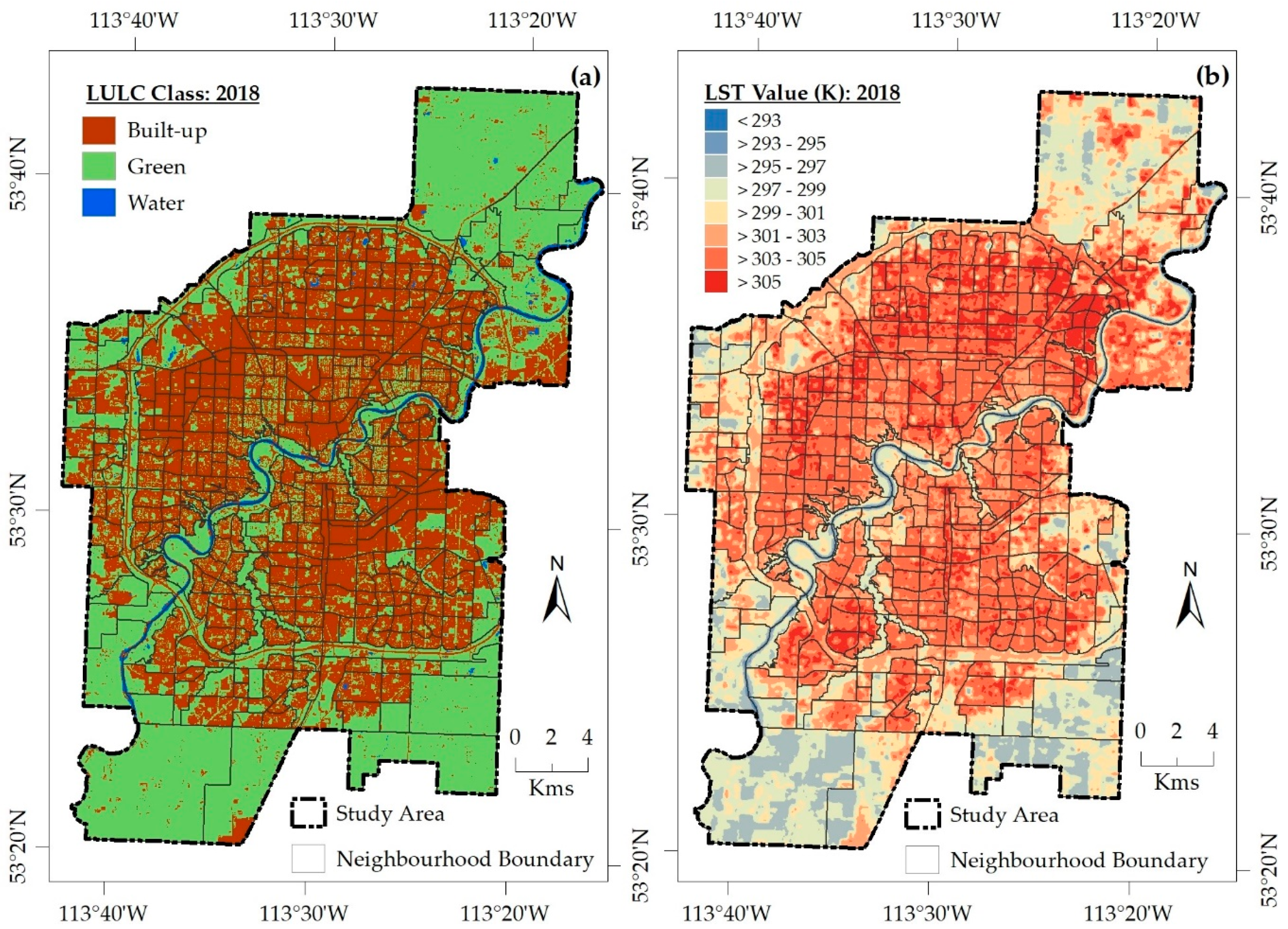
3.3. Analysis of the Influence of Structural Configurations on the LST at Neighbourhood Scale

In this analysis, we considered to apply spatial autocorrelation and proximity analysis. In order to execute the spatial autocorrelation method, we converted the rooflines vector data to raster with a spatial resolution of 2 m to capture all gaps among structures. In the study area, the minimum distance between two structures would be 2.4 m in the study area according to the regulations [35]. Next, we calculated local Moran’s I index, Ii(d)-values of raster data with 3 × 3 window, as follows [36]
I i ( d ) = Z i Z m i ( Z i Z m ) 2 j w i j ( d ) ( Z i Z m )
where Zi is the attribute value of interest at location i, Zm is the mean of the attribute Z values, wij (d) is a spatial weight matrix, and d (= 3 × 3) represents the size of the calculation window. The Ii(d)-values range from −1 to +1 for highly dispersed to clustered patterns, respectively. For the proximity analysis, we applied ‘near distance’ calculations on the rooflines vector data, on the basis of finding the shortest separation between two structures.
For analysing the influence of the structural configurations on the LST, we calculated zonal mean values of the both local Moran’s I and near distance for each subcategory of both industrial and residential neighbourhoods. Next, we used these mean values to carry out two sets of linear regression analyses between LST and (i) local Moran’s I index, (ii) near distance. In this case, we considered a set of three criteria: (i) use of residential and industrial neighbourhoods together, with the same percentages of combined water and green (e.g., I10 and R10 together); (ii) no use of I50+ and R50+ subcategories, because of their having more than 50% combined water and green; (iii) calculations of mean values using bins with a size of 0.03 and 5 m for local Moran’s I index and near distance, respectively.

4. Results

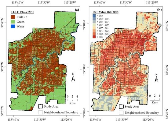
4.1. Evaluation of the LULC Maps and Dynamics of LST

We found the overall accuracies of 98.08%, 97.81%, and 98.53%; and kappa statistics of 0.95, 0.94, and 0.96 for the methods of ISODATA, RF, and indices-based respectively for 2018 (see Table 6). The best LULC map (i.e., indices-based) represented an area of 49.41%, 2.28%, and 48.32% for the built-up, water, and green classes, respectively (see Figure 3a). Furthermore, we estimated that the minimum, mean, and maximum LST were 286.08, 301.45, and 312.8 K, respectively. We observed the lower LST in and around the water and green LULC classes, and the higher LST in the built-up areas (see Figure 3b). For 2015, the overall accuracy and kappa statistics of the LULC map were found to be 97.90% and 0.92, respectively (see Table 6); and the estimated minimum, mean and maximum LST were 285.08, 296.08, and 302.88 K, respectively.

4.2. Relationships between LST and LULC Composition

The industrial, riverine/creek, freeway, agricultural, and residential categories consisted of 71, 27, 14, 25, and 263 neighbourhoods, respectively (see the Total column in Table 7; Figure 4a). Further, the number of subcategorized neighbourhoods of the industrial and residential are shown in the ‘subtotal’ columns of Table 7, and their spatial locations are shown in Figure 4b.
Our analysis revealed that the highest and lowest mean LST values were in the industrial and riverine/creek neighbourhood categories, respectively, where the values were very close to each other for the industrial and residential neighbourhoods (see 2nd and 3rd columns in Table 8). However, when the components of built-up, and combined green and water in the LULC composition were considered separately, we observed the highest and lowest mean LST values in the residential and riverine/creek categories, respectively (see 4th to 7th columns in Table 8).
The regression analysis between the mean LST values and neighbourhood subcategories of: (a) I10 to I50+, and (b) R10 to R50+, showed strong relationships, i.e., r2-values of ~0.90 and 0.35 for industrial, and ~0.95 and 0.52 for the residential subcategories, respectively (see Figure 5). Note that we used I10/R10 (=1) to I50+/R50+(=6) for the neighbourhood subcategory in the regression analysis. In all cases, the mean LST values were gradually decreasing with the increasing percentage of combined green and water component in the LULC composition. However, residential subcategories were showing higher mean LST values in comparison with the same composition of the industrial subcategories, which might be due to the differences in surface albedo characteristics as depicted in Figure 6a. In fact, we observed the higher albedo values (i.e., lower absorption of incident sunlight) in the industrial subcategories and considered this as one of the responsible factors for the relatively lower LST values when compared with the residential subcategories of neighbourhoods of both 2018 and 2015 (see Figure 6b).

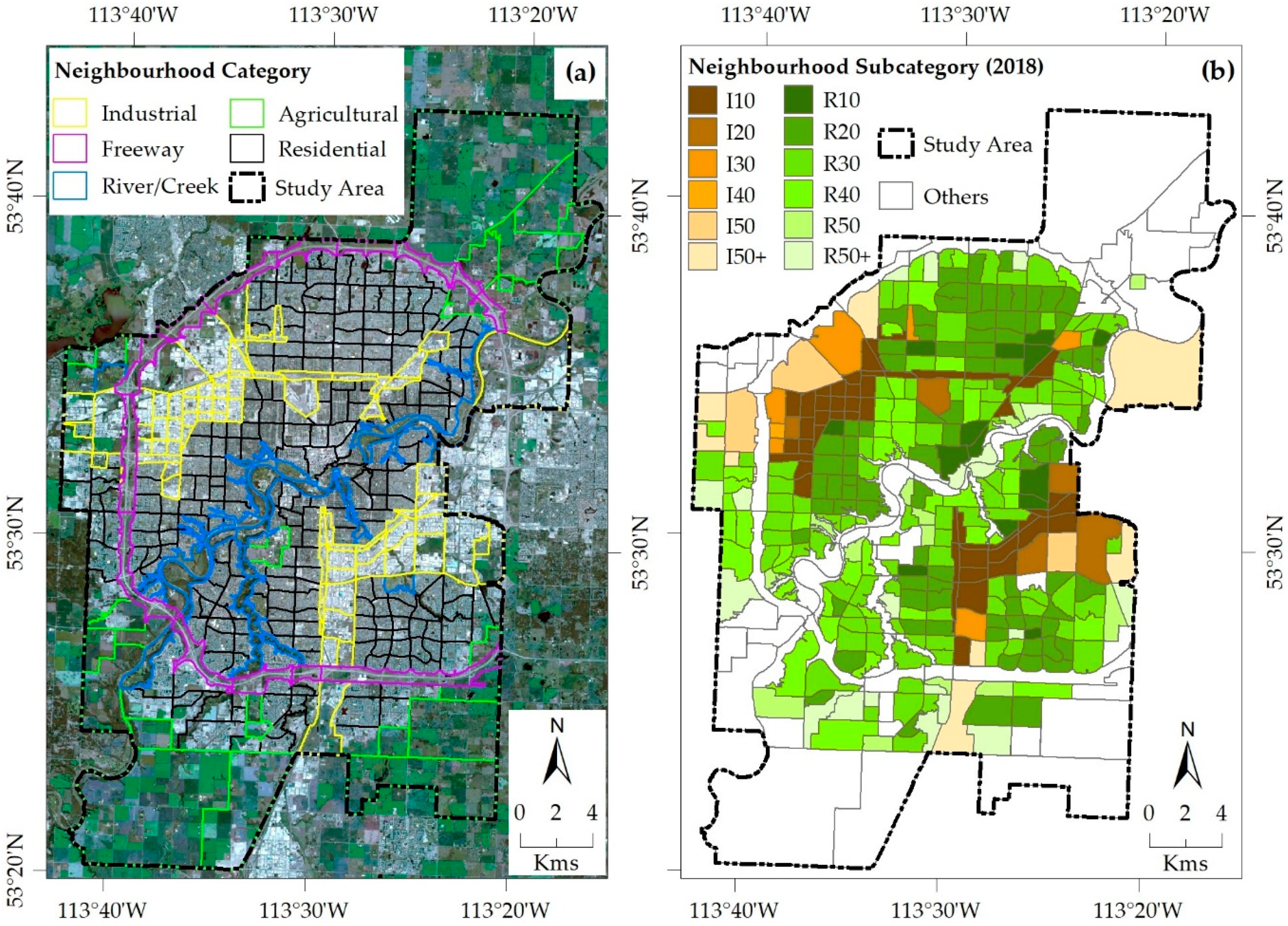
4.3. Influence of Structural Configurations on LST

The regression analysis between the mean LST values and the mean values of: (a) local Moran’s I index, and (b) near distance, were found to have reasonable agreements. For example: r2-values were in the range: (a) 0.49 to 0.74 (2018) and 0.22 to 0.96 (2015) for local Moran’s I, and (b) 0.47 to 0.88 (2018) and 0.42 to 1.0 (2015) for near distance analysis (see Table 9 for details). The negative slopes of the regressions (see 3rd and 6th columns in Table 9) indicated that the higher values of the both local Moran’s I and near distance would contribute to the lessening of LST values.

5. Discussion

Despite the similar overall accuracies (i.e., above 97%) and kappa statistics (i.e., above 94%) obtained from all the three classification methods in generating LULC maps, we preferred the indices-based LULC map for further analysis. This was due to the fact that this method would be simple and require less computational time in comparison to the RF and ISODATA clustering methods. In fact, our LULC map showed the green areas were in the neighbourhoods at the fringes of the city [37], which would be subject to continual development. Green areas were also found in neighbourhoods along the North Saskatchewan River, and other creeks, which were specifically developed for recreational parks and golf courses with no possibility of further developments [38]. Moreover, the central part of the city experienced the residential neighbourhoods’ establishment at least 50 years ago [39], therefore they would have more grown tree/vegetation around the structures. Additionally, the industrial neighbourhoods at the fringes of the city had more underdeveloped land consisting of more green LULC type in comparison to the neighbourhoods in the city core [40]. In general, the LULC composition in the study area showed the cluster-development of built-up areas in the city core, which was also reported in other studies [41,42,43].
Our results for the five different categories of neighbourhoods in the study area identified that both industrial and residential neighbourhoods exhibited high mean LST values compared to the other three neighbourhoods (i.e., riverine/creek, agricultural, and freeway). The industrial and residential neighbourhoods comprised a high density of built-up with impervious (artificial) surface probably causing higher LST values. Similar findings were also reported in Phoenix [7,14] and Las Vegas [44] cities of the United States. We also found lower mean LST values in the riverine/creek and agricultural neighbourhoods, where riverine/creek was the lowest. The neighbourhoods in the riverine/creek category consisted of over 80% green and water LULC classes, which probably had a strong cooling effect on the urban landscape [44], and thereby helped to lower the mean LST value. Additionally, agricultural neighbourhoods comprised agricultural lands with or without crops including some bare and exposed soils, which exhibited relatively higher LST in comparison to the riverine/creek ones. In fact, Ullah et al. [10] found that bare soil had higher LST values compared to water and vegetation, which might be similar to our riverine/creek category in terms of composition. Further, the freeway neighbourhood category comprised wider roads, grass, and bare lands; thus it showed a slightly higher mean LST value in comparison with riverine/creek and agricultural neighbourhoods that agreed quite well with the findings of Myint et al. [14].
Our analysis of the subcategories of both industrial and residential neighbourhoods revealed that the residential ones exhibited higher mean LST values with the same LULC composition as the industrial ones. In fact, our observations contradicted with other studies (e.g., [45,46]), because residential neighbourhoods ought to have lower LST compared to the industrial neighbourhoods. However, our albedo analysis, i.e., higher albedo values over the industrial subcategories to the residential ones, might be one of the potential explanations. Note that high albedo or the low absorption of incident sunlight was probably attributed to having rooftops with coated steels or metal sheets over the industrial neighbourhoods [47,48,49]. On the other hand, the rooftops/shingles in the residential neighbourhoods would be mainly made of asphalt with dark colour, so they might absorb more sunlight [49,50,51]. Consequently, they would exhibit higher LST values. In addition, the small distance of 2.4 m between structures in residential neighbourhoods probably facilitated densified clustered configuration. On the contrary, the dispersed configuration of industrial neighbourhoods with large open spaces and gaps between structures would create a large passage for wind flow that might help reducing the LST. This was also clear for local Moran’s I (as implemented elsewhere [7,14]) and proximity (near distance) analyses. Both analyses showed that the densified clustered configuration of the residential neighborhoods caused the high LST, while the dispersed configuration of industrial caused lower LST.

6. Conclusions

In this study, we demonstrated the influence of LULC composition and configuration on LST at the 400 neighbourhoods of the City of Edmonton. To aid this process, we generated LULC maps using Landsat-8 OLI image, and found that the indices-based method of LULC classification performed the best. Besides, we estimated an LST map from the Landsat-8 TIRS image with single-channel algorithm and observed that the built-up and water LULC classes showed the highest and lowest LST values, respectively. We further analysed the impacts of LULC composition on the five neighbourhood categories. We found that the industrial and riverine/creek neighbourhoods had the highest and lowest mean LST values, respectively, although industrial and residential showed very close values with a slight difference, i.e., 0.04 K (2018) and 0.57 K (2015). On the other hand, while we compared this with the subcategories of having same LULC composition in the residential and industrial neighbourhoods, we observed that the residential subcategories showed higher mean LST values. Such a high LST in the residential would be because of using the dark-coloured roof-top materials in the study area, as confirmed by our surface albedo analysis. Therefore, we suggest adopting light-coloured roof-top materials with high albedo properties in the residential structures. Further, local Moran’s I and proximity (near distance) analyses identified that structural configurations of cluster pattern would play a role in enhancing the LST.
Although our study explored the efficacy of Landsat data at the neighbourhood level, aerial photographs, or very high spatial resolution satellite image (e.g., less than 2 m) would explore further insight. Such images would facilitate generating a very high spatial resolution LULC composition to capture further details even between structures. This study would help policymakers, urban planners, and related stakeholders to have a clear understanding of the impacts of various landscape composition and structural configurations on surface energy balance in maintaining sustainable neighbourhoods in an urban setup. Despite the promising outcomes of this study, we strongly recommend evaluating the proposed method, and it should be investigated thoroughly before being applied in other cities.

Author Contributions

Conception and design, I.R.E., M.R.A., Q.K.H., A.D., A.G. and E.R.; Data processing and analysis, I.R.E. and M.R.A.; Methods, I.R.E., M.R.A., Q.K.H., A.D., A.G. and E.R.; Writing—original draft preparation, I.R.E. and M.R.A.; Writing—review and editing, Q.K.H., A.D., A.G. and E.R.; Supervision, Q.K.H. All authors have read and agreed to the published version of the manuscript.

Funding

The study was partially funded by: (i) Tertiary Education Trust Fund (TETFUND) of Nigeria to I. Ejiagha; and (ii) NSERC DG to Q. Hassan.

Acknowledgments

We would like to thank USGS and Google for providing Landsat-8 and Google Earth images respectively with free of cost. We also acknowledge the City of Edmonton for providing vector layers used in this study.

Conflicts of Interest

The authors declare no conflict of interest. The funders had no role in the design of the study; in the collection, analyses, or interpretation of data; in the writing of the manuscript, or in the decision to publish the results.

References

  1. United Nations Secretariat World Urbanization Prospects. The 2001 Revision. Data Tables and Highlights. Available online: http://www.megacities.uni-koeln.de/documentation/megacity/statistic/wup2001dh.pdf (accessed on 29 June 2020).
  2. United Nations. World Urbanization Prospects: The 2018 Revision. Available online: https://population.un.org/wup/Publications/Files/WUP2018-Report.pdf (accessed on 29 June 2020).
  3. Wu, Z.; Zhang, Y. Spatial Variation of Urban Thermal Environment and Its Relation to Green Space Patterns: Implication to Sustainable Landscape Planning. Sustainability 2018, 10, 2249. [Google Scholar] [CrossRef] [Green Version]
  4. Mukherjee, S.; Joshi, P.K.; Garg, R.D. Analysis of urban built-up areas and surface urban heat island using downscaled MODIS derived land surface temperature data. Geocarto Int. 2017, 32, 900–918. [Google Scholar] [CrossRef]
  5. Shahmohamadi, P.; Che-Ani, A.I.; Maulud, K.N.A.; Tawil, N.M.; Abdullah, N.A.G. The Impact of Anthropogenic Heat on Formation of Urban Heat Island and Energy Consumption Balance. Urban Stud. Res. 2011, 2011. [Google Scholar] [CrossRef] [Green Version]
  6. Osborne, B.P.; Osborne, V.J.; Kruger, M.L. Comparison of satellite surveying to traditional surveying methods for the resources industry. JBIS—J. Br. Interplanet. Soc. 2012, 65, 98–104. [Google Scholar]
  7. Connors, J.P.; Galletti, C.S.; Chow, W.T.L. Landscape configuration and urban heat island effects: Assessing the relationship between landscape characteristics and land surface temperature in Phoenix, Arizona. Landsc. Ecol. 2013, 28, 271–283. [Google Scholar] [CrossRef]
  8. Afrin, S.; Gupta, A.; Farjad, B.; Razu Ahmed, M.; Achari, G.; Hassan, Q. Development of land-use/land-cover maps using landsat-8 and MODIS data, and their integration for hydro-ecological applications. Sensors 2019, 19, 4891. [Google Scholar] [CrossRef] [Green Version]
  9. Akbar, T.A.; Hassan, Q.K.; Ishaq, S.; Batool, M.; Butt, H.J.; Jabbar, H. Investigative Spatial Distribution and Modelling of Existing and Future Urban Land Changes and Its Impact on Urbanization and Economy. Remote Sens. 2019, 11, 105. [Google Scholar] [CrossRef] [Green Version]
  10. Ullah, S.; Tahir, A.A.; Akbar, T.A.; Hassan, Q.K.; Dewan, A.; Khan, A.J.; Khan, M. Remote Sensing—Based Quantification of the Relationships between Land Use Land Cover Changes and Surface Temperature over the Lower Himalayan Region. Sustainability 2019, 11, 5492. [Google Scholar] [CrossRef] [Green Version]
  11. Abdullah, A.Y.M.; Masrur, A.; Gani Adnan, M.S.; Al Baky, M.A.; Hassan, Q.K.; Dewan, A. Spatio-temporal patterns of land use/land cover change in the heterogeneous coastal region of Bangladesh between 1990 and 2017. Remote Sens. 2019, 11, 790. [Google Scholar] [CrossRef] [Green Version]
  12. Zhao, Z.Q.; He, B.J.; Li, L.G.; Wang, H.B.; Darko, A. Profile and concentric zonal analysis of relationships between land use/land cover and land surface temperature: Case study of Shenyang, China. Energy Build. 2017, 155, 282–295. [Google Scholar] [CrossRef]
  13. Hua, A.K.; Ping, O.W. The influence of land-use/land-cover changes on land surface temperature: A case study of Kuala Lumpur metropolitan city. Eur. J. Remote Sens. 2018, 51, 1049–1069. [Google Scholar] [CrossRef] [Green Version]
  14. Myint, S.W.; Zheng, B.; Talen, E.; Fan, C.; Kaplan, S.; Middel, A.; Smith, M.; Huang, H.; Brazel, A. Does the spatial arrangement of urban landscape matter? Examples of urban warming and cooling in phoenix and las vegas. Ecosyst. Heal. Sustain. 2015, 1, 1–15. [Google Scholar] [CrossRef]
  15. Zheng, B.; Myint, S.W.; Fan, C. Spatial configuration of anthropogenic land cover impacts on urban warming. Landsc. Urban Plan. 2014, 130, 104–111. [Google Scholar] [CrossRef]
  16. Rhee, J.; Park, S.; Lu, Z. Relationship between land cover patterns and surface temperature in urban areas. GIScience Remote Sens. 2014, 51, 521–536. [Google Scholar] [CrossRef]
  17. Li, J.; Song, C.; Cao, L.; Zhu, F.; Meng, X.; Wu, J. Impacts of landscape structure on surface urban heat islands: A case study of Shanghai, China. Remote Sens. Environ. 2011, 115, 3249–3263. [Google Scholar] [CrossRef]
  18. Weng, Q.; Liu, H.; Lu, D. Assessing the effects of land use and land cover patterns on thermal conditions using landscape metrics in city of Indianapolis, United States. Urban Ecosyst. 2007, 10, 203–219. [Google Scholar] [CrossRef]
  19. Fan, C.; Wang, Z. Spatiotemporal characterization of land cover impacts on urban warming: A spatial autocorrelation approach. Remote Sens. 2020, 12, 1631. [Google Scholar] [CrossRef]
  20. Wu, X.; Li, B.; Li, M.; Guo, M.; Zang, S.; Zhang, S. Examining the Relationship Between Spatial Configurations of Urban Impervious Surfaces and Land Surface Temperature. Chinese Geogr. Sci. 2019, 29, 568–578. [Google Scholar] [CrossRef] [Green Version]
  21. The City of Red Deer. Neighbourhood Planning & Design Standards. Available online: https://www.reddeer.ca/media/reddeerca/business-in-red-deer/planning-and-development-of-property/planning/Neighbourhood-Planning--Design-Standards-combined-June-2015.pdf (accessed on 29 June 2020).
  22. The City of Edmonton. Designing New Neighbourhoods. Guidelines for Edmonton’s Future Residential Communities. Available online: https://www.edmonton.ca/documents/PDF/Designing_New_Neighbourhoods_Final.pdf (accessed on 29 June 2020).
  23. The City of Edmonton. Facts & Figures. Available online: https://www.edmonton.ca/city_government/facts-figures.aspx (accessed on 18 May 2020).
  24. Government of Canada. 1981–2010 Climate Normals & Averages. Available online: https://climate.weather.gc.ca/climate_normals/ (accessed on 18 May 2020).
  25. USGS. EarthExplorer—Home. Available online: http://earthexplorer.usgs.gov/ (accessed on 20 May 2020).
  26. The City of Edmonton. City of Edmonton’s Open Data Portal. Available online: https://data.edmonton.ca/ (accessed on 19 May 2020).
  27. Ahmed, M.R.; Rahaman, K.R.; Kok, A.; Hassan, Q.K. Remote sensing-based quantification of the impact of flash flooding on the rice production: A case study over Northeastern Bangladesh. Sensors 2017, 17, 2347. [Google Scholar] [CrossRef] [Green Version]
  28. Mosleh, M.K.; Hassan, Q.K. Development of a remote sensing-based “boro” rice mapping system. Remote Sens. 2014, 6, 1938–1953. [Google Scholar] [CrossRef] [Green Version]
  29. Rouse, J.W.; Haas, R.H.; Schell, J.A.; Deering, D.W. Monitoring vegetation systems in the Great Plains with ERTS. In Third Earth Resources Technology Satellite-1 Symposium; NASA Special Publication 351: Washington, DC, USA, 1973; pp. 309–317. [Google Scholar]
  30. Xu, H. Modification of normalised difference water index (NDWI) to enhance open water features in remotely sensed imagery. Int. J. Remote Sens. 2006, 27, 3025–3033. [Google Scholar] [CrossRef]
  31. Zha, Y.; Gao, J.; Ni, S. Use of normalized difference built-up index in automatically mapping urban areas from TM imagery. Int. J. Remote Sens. 2003, 24, 583–594. [Google Scholar] [CrossRef]
  32. Avdan, U.; Jovanovska, G. Algorithm for Automated Mapping of Land Surface Temperature Using LANDSAT 8 Satellite Data. J. Sens. 2016, 2016. [Google Scholar] [CrossRef] [Green Version]
  33. Sobrino, J.A.; Jiménez-Muñoz, J.C.; Paolini, L. Land surface temperature retrieval from LANDSAT TM 5. Remote Sens. Environ. 2004, 90, 434–440. [Google Scholar] [CrossRef]
  34. Baldinelli, G.; Bonafoni, S.; Rotili, A. Albedo Retrieval from Multispectral Landsat 8 Observation in Urban Environment: Algorithm Validation by in situ Measurements. IEEE J. Sel. Top. Appl. Earth Obs. Remote Sens. 2017, 10, 4504–4511. [Google Scholar] [CrossRef]
  35. The City of Edmonton. Edmonton Zoning Bylaw 12800; City of Edmonton: Edmonton, AB, Canada, 2017. [Google Scholar]
  36. Anselin, L. Local Indicators of Spatial Association—LISA. Geogr. Anal. 1995, 27, 93–115. [Google Scholar] [CrossRef]
  37. Apparicio, P.; Pham, T.T.H.; Séguin, A.M.; Dubé, J. Spatial distribution of vegetation in and around city blocks on the Island of Montreal: A double environmental inequity? Appl. Geogr. 2016, 76, 128–136. [Google Scholar] [CrossRef] [Green Version]
  38. Mittal, J.; Byahut, S. Value Capitalization Effects of Golf Courses, Waterfronts, Parks, Open Spaces, and Green Landscapes—A Cross-Disciplinary Review. J. Sustain. Real Estate 2016, 8, 62–94. [Google Scholar]
  39. The City of Edmonton. Mature Neighbourhoods. Edmonton—Open Data Portal. Available online: https://data.edmonton.ca/Geospatial-Boundaries/Mature-Neighbourhoods-Map/3jmw-i9z8 (accessed on 29 June 2020).
  40. The City of Edmonton. Vacant Industrial Land Supply: Urban Form and Corporate Strategic Development City Planning; City of Edmonton: Edmonton, AB, Canada, 2018. [Google Scholar]
  41. Stiles, R.; Gasienica-wawrytko, B.; Hagen, K.; Loibl, W.; Tötzer, T.; Köstl, M.; Pauleit, S.; Schirmann, A.; Felmayr, W.; Trimmel, H. Understanding the whole city as landscape. A multivariate approach to urban landscape morphology. SPOOL 2014, 1, 401–418. [Google Scholar]
  42. Mustafa, A.; Heppenstall, A.; Omrani, H.; Saadi, I.; Cools, M.; Teller, J. Modelling built-up expansion and densification with multinomial logistic regression, cellular automata and genetic algorithm. Comput. Environ. Urban Syst. 2018, 67, 147–156. [Google Scholar] [CrossRef] [Green Version]
  43. Zhen, F.; Qin, X.; Ye, X.; Sun, H.; Luosang, Z. Analyzing urban development patterns based on the flow analysis method. Cities 2019, 86, 178–197. [Google Scholar] [CrossRef]
  44. Zhou, W.; Huang, G.; Cadenasso, M.L. Does spatial configuration matter? Understanding the effects of land cover pattern on land surface temperature in urban landscapes. Landsc. Urban Plan. 2011, 102, 54–63. [Google Scholar] [CrossRef]
  45. Kim, J.; Gu, D.; Sohn, W.; Kil, S.; Kim, H.; Lee, D. Neighborhood Landscape Spatial Patterns and Land Surface Temperature: An Empirical Study on Single-Family Residential Areas in Austin, Texas. Int. J. Environ. Res. Public Health 2016, 13, 880. [Google Scholar] [CrossRef] [PubMed] [Green Version]
  46. Fikfak, A.; Kosanovi, S.; Konjar, M.; Grom, J.; Zbašnik-senegă, M. The Impact of Morphological Features on Summer Temperature Variations on the Example of Two Residential Neighborhoods in Ljubljana, Slovenia. Sustainability 2017, 9, 122. [Google Scholar] [CrossRef] [Green Version]
  47. Vox, G.; Maneta, A.; Schettini, E. Evaluation of the radiometric properties of roofing materials for livestock buildings and their effect on the surface temperature. Biosyst. Eng. 2016, 144, 26–37. [Google Scholar] [CrossRef]
  48. Rossi, S.; Calovi, M.; Dalpiaz, D.; Fedel, M. The Influence of NIR Pigments on Coil Coatings’ Thermal Behaviors. Coatings 2020, 10, 514. [Google Scholar] [CrossRef]
  49. CLM Steel Roofing Edmonton. Benefits of Metal Roofing Over a Shingle Roof. Available online: https://clmmetalroofsalberta.ca/benefits-of-metal-roofing-over-a-shingle-roof/ (accessed on 29 June 2020).
  50. A. Clark Roofing & Siding LP. Factors to Consider When Choosing a Shingle Colour. Available online: https://www.aclark.ca/blog/factors-consider-choosing-shingle-colour/ (accessed on 18 June 2020).
  51. Akbari, H.; Kolokotsa, D. Three decades of urban heat islands and mitigation technologies research. Energy Build. 2016, 133, 834–842. [Google Scholar] [CrossRef]
Figure 1. Study area showing the City of Edmonton’s extent in the Canadian Province of Alberta, where the city comprises of 400 neighbourhoods. The boundaries of these neighbourhoods were overlaid on a Landsat-8 OLI image with a false colour composite (RGB:543) acquired on 07 September 2018.
Remotesensing 12 02508 g001
Figure 2. Schematic diagram of the proposed methods in the scope of this study.
Remotesensing 12 02508 g002
Figure 3. (a) Indices-based LULC map showing the spatial distribution of the three LULC classes (2018), where the built-up is located in the core surrounded by the green at the fringes, and the major water portion is the river that passes across diagonally from southwest to northeast in the middle; and (b) the LST map (2018) representing the temperature variations over the study area, where the higher LST are located in the built-up, and the lower LST are along the green and water classes.
Remotesensing 12 02508 g003
Figure 4. (a) Map showing the neighbourhoods grouped into five different categories, overlaid on the Landsat-8 OLI image (2018) with a natural colour composite (RGB:432); and (b) map showing the 12 subcategories of the neighbourhoods (2018), where ‘I’ represents the industrial and ‘R’ represents the residential categories.
Remotesensing 12 02508 g004
Figure 5. A scatterplot of the mean LST values comparing the two subcategory sets of industrial and residential neighbourhood categories for both 2018 (late summer) and 2015 (early spring), where each set consists with six subcategories. The linear regression coefficients of the both neighbourhood categories are representing the relations of mean surface temperature with the configuration of the subcategories of the neighbourhoods.
Remotesensing 12 02508 g005
Figure 6. (a) Map showing the estimated values of surface albedo (2018), where the red to reddish colour tones represent the higher albedo values in compared to the lower albedo values represented by the blue to bluish. The yellow to yellowish colours represent the medium level of albedo; (b) surface albedo of subcategorized industrial neighbourhoods indicated high surface albedo (both 2018 and 2015), while low surface albedo for residential subcategories (both 2018 and 2015).
Remotesensing 12 02508 g006
Table 1. Example case studies that explored relations between landscape configuration and LST.
CategoryRef.Description *
Fragmentation metricsLi et al. [17]
  • Used aerial photo-derived LULC map at 2.5 m, and Landsat ETM+-derived LST at 60 m over Shanghai, China
  • Considered five LULC class-level metrics, i.e., PLAND, PD, ED, LSI, and CLUMPY; and six landscape-level metrics, i.e., PD, ED, LSI, CONTAG, SHDI, and SHEI
  • Obtained r2-values in the range: (i) 0.001 to 0.394 for class-level metrics, and (ii) 0.066 to 0.416 for landscape-level metrics
Connors et al. [7]
  • Employed QuickBird-derived LULC map at 2.4 m, and ASTER-estimated LST at 90 m over Phoenix, United States
  • Applied five LULC class-level metrics, i.e., PLAND, PD, ED, LSI, and FRAC_AM; and six landscape-level metrics, i.e., PD, ED, LSI, FRAC_AM, CONTAG, and SHDI
  • Obtained r2-values for class-level metrics in the range: (i) 0.010 to 0.397 for Mesic residential, (ii) 0.001 to 0.078 for Xeric residential, and (iii) 0.003 to 0.410
Wu and Zhang [3]
  • Used Landsat 8-derived LULC map at 30 m, and LST at 100 m Suzhou, China
  • Examined four LULC class-level metrics, i.e., MPS, SI, AI, and FD
  • Achieved r2-values in the range 0.054 to 0.422
Spatial autocorrelationZheng et al. [15]
  • Applied QuickBird-derived LULC map at 2.4 m and ASTER (daytime and nighttime) estimated LST at 90 m over Phoenix, United States
  • Used local Moran’s I, and achieved r2-values between: (i) 0.04 and 0.02 for building, and (ii) 0.17 and 0.38 for paved surfaces
Myint et al. [14]
  • Employed QuickBird and GeoEye-1 at 2.4 m and 3.0 m respectively to derived LULC maps, with ASTER (daytime and nighttime) estimated LST at 90 m over Phoenix and Las Vegas, United States
  • Applied local Moran’s I, and attained r2-values in the range: (i) 0.078 to 0.397 for daytime LST and 0.006 to 0.260 for nighttime LST in Las Vegas, and (ii) 0.040 to 0.410 for daytime LST and 0.020 to 0.436 nighttime LST in Phoenix
Wu et al. [20]
  • Used Landsat TM-derived impervious surface area (ISA) maps at 30 m, and TM thermal band at 120 m over Harbin, China
  • Considered local Moran’s I, and obtained r2-values of 0.021 and 0.042 for year 2000 and 2010 respectively
* PLAND: percentage landscape area, SHEI: Shannon’s Evenness index, SHDI: Shannon’s Diversity index, ED: edge density, PD: patch density, LSI: landscape index, CI: clumpiness index, CONTAG: contagion, FRAC_AM: fractal dimension, MPS: mean plaque size, SI: shape index, AI: aggregation index, FD: fragmentation index, ASTER: advanced spaceborne thermal emission and reflection radiometer, TM: thematic mapper, ETM+: enhanced thematic mapper plus.
Table 2. Characteristics of the Landsat-8 images used in this study, and its usages.
Landsat-8 SensorProduct and Spatial ResolutionBand Number and NameWavelength (μm)Utilization
OLISurface reflectance
(30 m)
B1: Coastal aerosol0.43–0.45Albedo estimation *
and
LULC classification *
B2: Blue0.45–0.51
B3: Green0.53–0.59
B4: Red0.64–0.67
B5: Near Infrared, NIR0.85–0.88
B6: Shortwave Infrared 1 (SWIR1)1.57–1.65
B7: Shortwave Infrared 2 (SWIR2)2.11–2.29
TIRSBrightness temperature (30 m) **B10: Thermal Infrared 1 (TIR1)10.60–11.19Surface temperature
estimation
* Seven OLI bands were used to estimate albedo; however, six bands (excluding the coastal aerosol one) were used for LULC classification. ** Resampled by USGS from original 100 m resolution.
Table 3. Description of the LULC classes.
LULC ClassDescription
Built-upDevelopments in urban including residential areas, impervious surfaces (bitumen and concrete), and industrial areas.
WaterOpen water bodies including the river, creeks, lakes, and pools (both natural and artificial).
Green Vegetation (including grasses, shrubs, and trees), agricultural lands (with and without crops), bare surfaces, and open spaces.
Table 4. Criteria used for grouping the neighbourhoods into five different categories.
CategoryCriteria for Categorization
IndustrialHaving ‘industrial’ word in the name attribute, large structural footprints, and occupied more than 50% of a neighbourhood.
Riverine/creekHaving word ‘river’ or ‘creek’ in the attribute, recreational park, golf course, and located along river and creek with vegetation canopy.
FreewayRoads with the words ‘Anthony Henday’ in the attribute.
Agricultural More than 50% agricultural land, bare land, and open space.
ResidentialRemaining neighbourhoods.
Table 5. Criteria used for the subcategorization of the industrial and residential neighbourhoods.
Neighbourhood SubcategoryWater and Green Combined (%)
IndustrialResidential
I10R10≤10
I20R20>10 to ≤20
I30R30>20 to ≤30
I40R40>30 to ≤40
I50R50>40 to ≤50
I50+R50+>50
Table 6. Comparison of the accuracy assessments of the classified LULC maps.
Classification MethodUser Accuracy (%)Producer Accuracy (%)Overall Accuracy (%)Kappa Statistic
ISODATA98.0698.1698.080.95
RF97.6998.0797.810.94
Indices-based *98.7394.7998.530.96
Indices-based **98.1496.3997.900.92
* 2018 image; ** 2015 image.
Table 7. Number of neighbourhoods in different categories and subcategories.
CategorySubcategorySubtotal
(2018)
Subtotal
(2015)
TotalPercent
IndustrialI1049307117.75
I20520
I3065
I4016
I5032
I50+78
ResidentialR1014526365.75
R208664
R308486
R404551
R501420
R50+2037
Riverine/creek---276.75
Freeway---143.5
Agricultural---256.25
Grand total 400100
Table 8. Dynamics of the mean LST in the scale of neighbourhood and composition.
CategoryMean LST (K)
Neighbourhood ScaleComponent
Built-UpGreen and Water
201820152018201520182015
Industrial303.51295.99303.76296.10302.55296.03
Residential303.47296.56303.81296.75302.75296.32
Freeway301.55292.24302.26295.21301.45295.59
Agricultural299.02293.95300.68294.43298.92296.21
Riverine/Creek298.77292.89299.79293.21298.56292.77
Table 9. Linear regression analysis between the mean LST values and mean values of (a) local Moran’s I, and (b) near distance for the neighbourhood subcategories.
YearNeighbourhood SubcategoryNumber of SamplesLinear Regression
(a) LST and Local Mean’s I(b) LST and Near Distance
SlopeIntercept (K)r2SlopeIntercept (K)r2
2018I10/R1063−2.5217304.920.66−0.0221304.580.47
I20/R2091−21.304308.520.52−0.1088304.540.66
I30/R3090−7.1125304.930.74−0.071304.480.49
I40/R4046−7.7945304.420.52−0.0504302.970.88
I50/R5017−10.315303.760.49−0.0871302.120.85
2015I10/R1035−0.4812296.660.22−0.0322296.960.92
I20/R2084−6.3835298.050.79−0.0742297.040.99
I30/R3091−23.995301.680.78−0.0699297.430.42
I40/R4057−10.365298.570.96−0.1131297.480.90
I50/R50226.6447295.060.42−0.0358296.481.00

