Generating a Spatio-Temporal Complete 30 m Leaf Area Index from Field and Remote Sensing Data

 , , and
Abstract
:
1. Introduction
2. Data and Methods
2.1. Research Area
2.2. Data Preprocessing
2.2.1. Landsat Data
2.2.2. MODIS LAI Product
2.2.3. Field Data
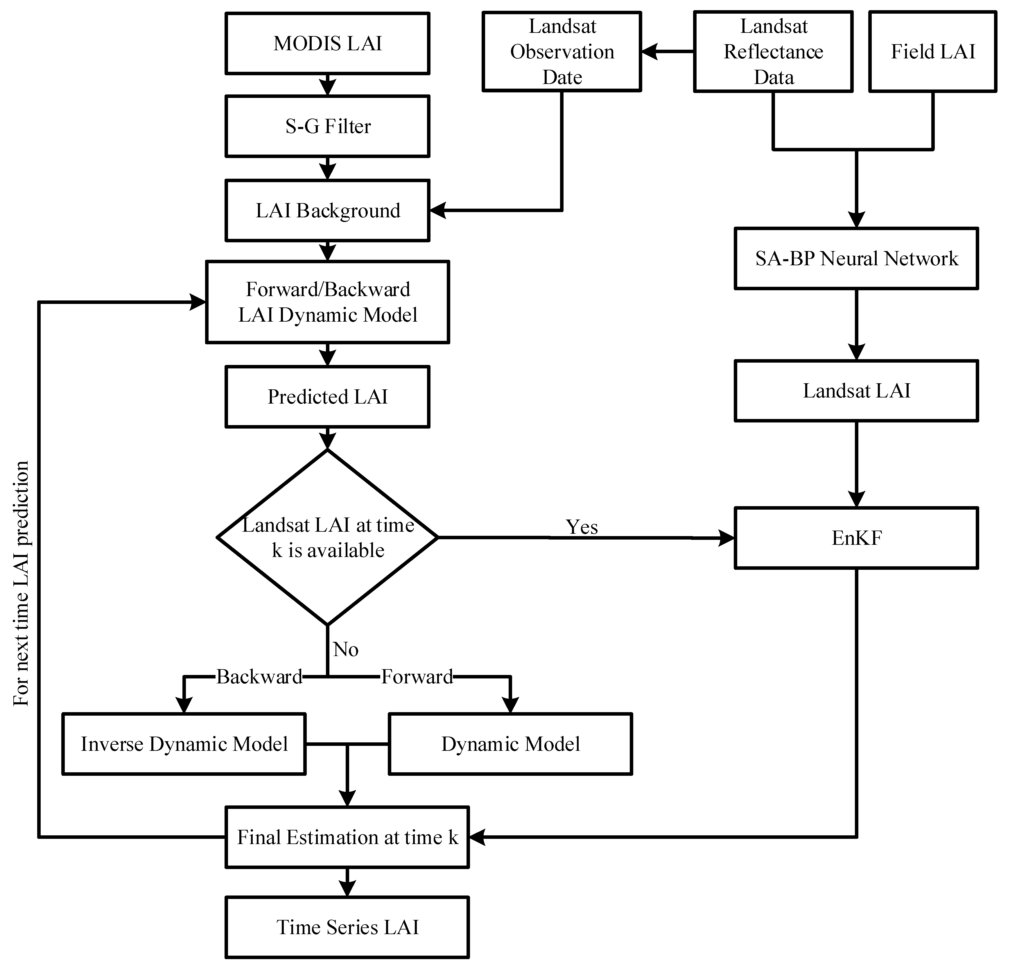
3. Method
3.1. Landsat LAI Estimation
3.2. LAI Dynamic Model Construction
3.3. MEnKF Assimilation Algorithm
4. Results
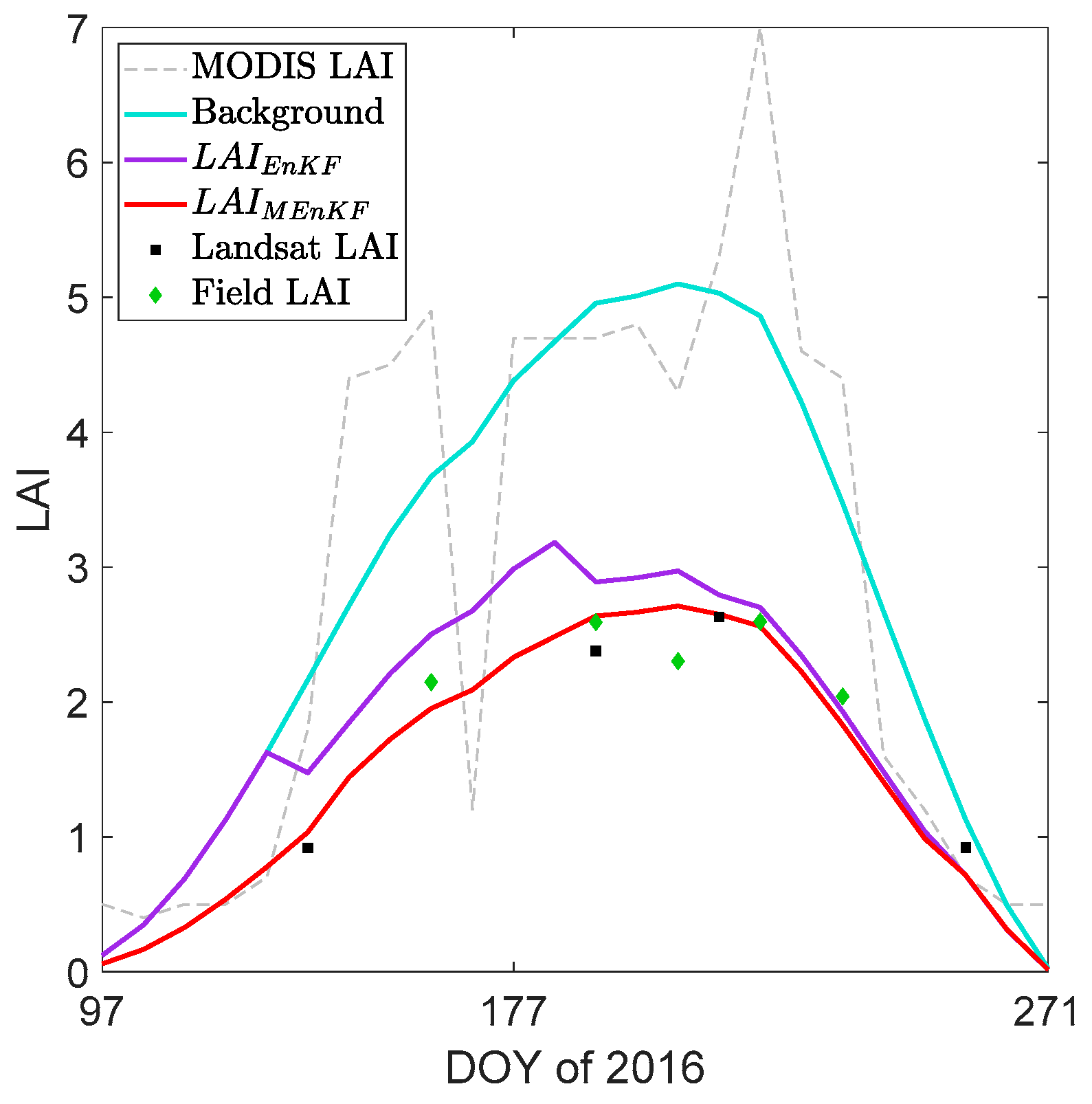
4.1. Single-Point Time Series LAI Validation
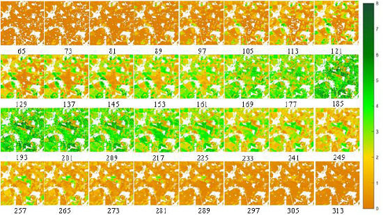
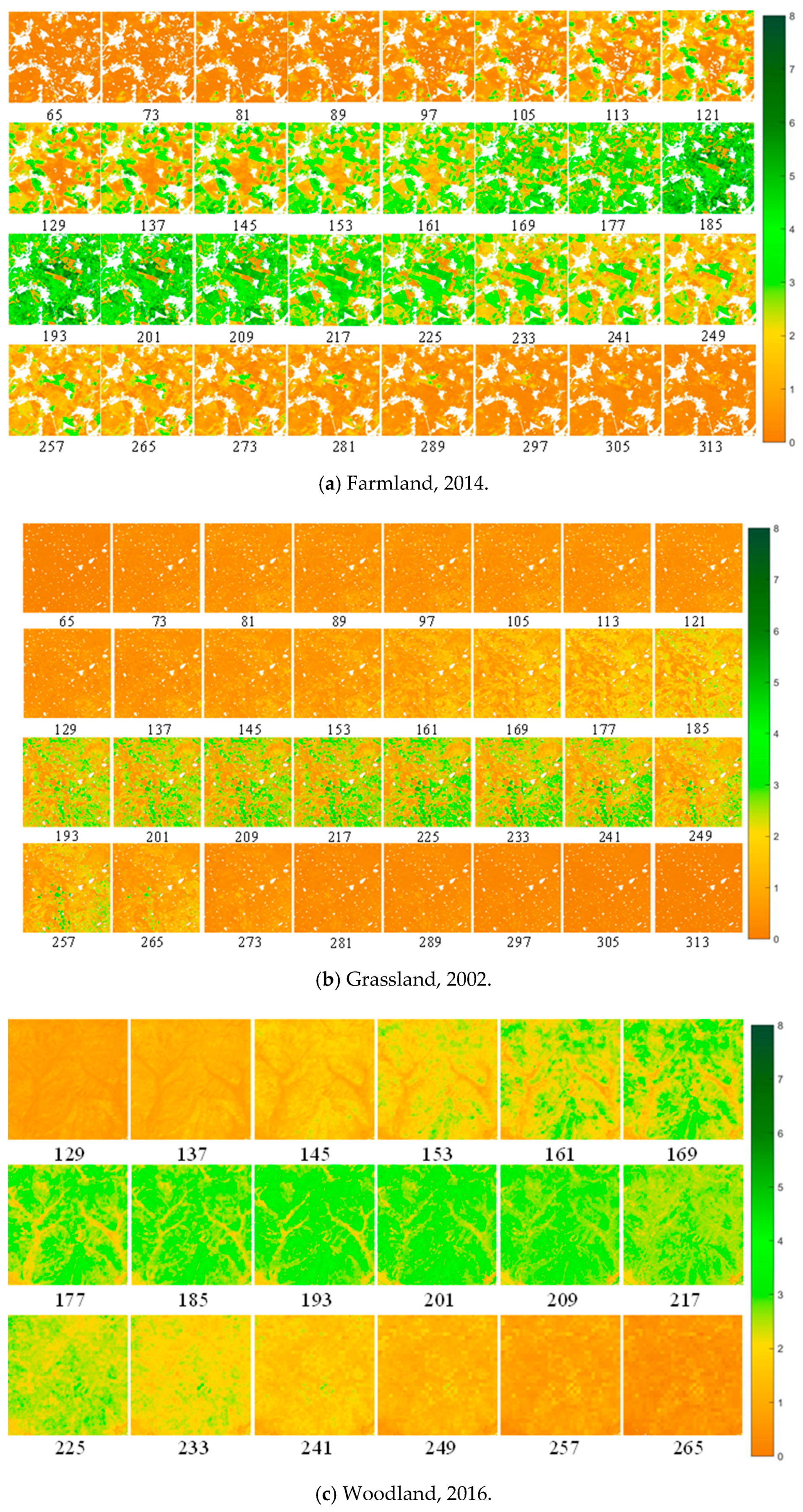
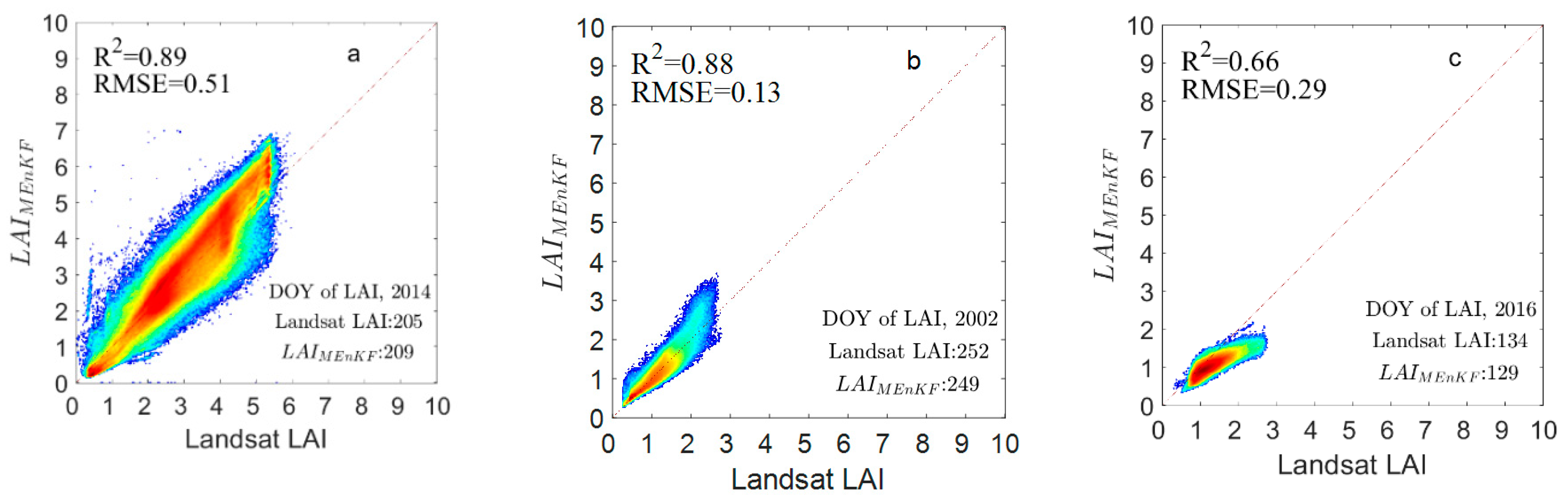
4.2. Regional LAI Validation
5. Discussion
5.1. Error Induced by Landsat LAI
5.2. Error Induced by the LAI Background
5.3. Advance of Assimilation from the LAI Peak Position
5.4. Extendibility of MEnKF
6. Conclusions
Author Contributions
Funding
Acknowledgments
Conflicts of Interest
References
- Chen, J.M.; Black, T.A. Defining leaf area index for non-flat leaves. Plant Cell Environ. 1992, 15, 421–429. [Google Scholar] [CrossRef]
- Cleugh, H.A.; Leuning, R.; Mu, Q.; Running, S.W. Regional evaporation estimates from flux tower and MODIS satellite data. Remote Sens. Environ. 2007, 106, 285–304. [Google Scholar] [CrossRef]
- Liu, Y.; Liu, R.; Chen, J.M. Retrospective retrieval of long-term consistent global leaf area index (1981–2011) from combined AVHRR and MODIS data. J. Geophys. Res. Biogeosci. 2012, 117. [Google Scholar] [CrossRef]
- Laurance, W.F.; Laurance, S.G.; Delamonica, P. Tropical forest fragmentation and greenhouse gas emissions. For. Ecol. Manag. 1998, 110, 173–180. [Google Scholar] [CrossRef]
- Omer, G.; Mutanga, O.; Abdel-Rahman, E.M.; Adam, E. Empirical prediction of leaf area index (LAI) of endangered tree species in intact and fragmented indigenous forests ecosystems using WorldView-2 data and two robust machine learning algorithms. Remote Sens. 2016, 8, 324. [Google Scholar] [CrossRef] [Green Version]
- Zheng, G.; Moskal, L.M. Retrieving leaf area index (LAI) using remote sensing: Theories, methods and sensors. Sensors 2009, 9, 2719–2745. [Google Scholar] [CrossRef] [Green Version]
- Jonckheere, I.; Fleck, S.; Nackaerts, K.; Muys, B.; Coppin, P.; Weiss, M.; Baret, F. Review of methods for in situ leaf area index determination: Part I. Theories, sensors and hemispherical photography. Agric. For. Meteorol. 2004, 121, 19–35. [Google Scholar] [CrossRef]
- Myneni, R.B.; Hoffman, S.; Knyazikhin, Y.; Privette, J.; Glassy, J.; Tian, Y.; Wang, Y.; Song, X.; Zhang, Y.; Smith, G. Global products of vegetation leaf area and fraction absorbed PAR from year one of MODIS data. Remote Sens. Environ. 2002, 83, 214–231. [Google Scholar] [CrossRef] [Green Version]
- Yan, K.; Park, T.; Yan, G.; Liu, Z.; Yang, B.; Chen, C.; Nemani, R.; Knyazikhin, Y.; Myneni, R. Evaluation of MODIS LAI/FPAR product collection 6. Part 2: Validation and intercomparison. Remote Sens. 2016, 8, 460. [Google Scholar] [CrossRef] [Green Version]
- Knyazikhin, Y.; Martonchik, J.V.; Myneni, R.B.; Diner, D.J.; Running, S.W. Estimating vegetation canopy leaf area index and fraction of absorbed photosynthetically active radiation from MODIS and MISR data. J. Geophys. Res. Space Phys. 1998, 103, 32257–32275. [Google Scholar] [CrossRef] [Green Version]
- Baret, F.; Hagolle, O.; Geiger, B.; Bicheron, P.; Miras, B.; Huc, M.; Berthelot, B.; Niño, F.; Weiss, M.; Samain, O. LAI, fAPAR and fCover CYCLOPES global products derived from VEGETATION: Part 1: Principles of the algorithm. Remote Sens. Environ. 2007, 110, 275–286. [Google Scholar] [CrossRef] [Green Version]
- Claverie, M.; Matthews, J.; Vermote, E.; Justice, C. A 30+ Year AVHRR LAI and FAPAR Climate Data Record: Algorithm Description and Validation. Remote Sens. 2016, 8, 263. [Google Scholar] [CrossRef] [Green Version]
- Zhang, Y.; Tian, Y.; Knyazikhin, Y.; Martonchik, J.V.; Diner, D.J.; Leroy, M.; Myneni, R.B. Prototyping of MISR LAI and FPAR algorithm with POLDER data over Africa. IEEE Trans. Geosci. Remote Sens. 2000, 38, 2402–2418. [Google Scholar] [CrossRef] [Green Version]
- Baret, F.; Weiss, M.; Lacaze, R.; Camacho, F.; Makhmara, H.; Pacholcyzk, P.; Smets, B. GEOV1: LAI and FAPAR essential climate variables and FCOVER global time series capitalizing over existing products. Part1: Principles of development and production. Remote Sens. Environ. 2013, 137, 299–309. [Google Scholar] [CrossRef]
- Xiao, Z.; Liang, S.; Wang, J.; Chen, P.; Yin, X.; Zhang, L.; Song, J. Use of General Regression Neural Networks for Generating the GLASS Leaf Area Index Product From Time-Series MODIS Surface Reflectance. IEEE Trans. Geosci. Remote Sens. 2013, 52, 209–223. [Google Scholar] [CrossRef]
- Liang, S.; Xiang, Z.; Liu, S.; Yuan, W.; Xiao, C.; Xiao, Z.; Zhang, X.; Qiang, L.; Jie, C.; Tang, H. A long-term Global Land Surface Satellite (GLASS) data-set for environmental studies. Int. J. Digit. Earth. 2013, 6, 5–33. [Google Scholar] [CrossRef]
- Yao, X.; Wang, N.; Liu, Y.; Cheng, T.; Tian, Y.; Chen, Q.; Zhu, Y. Estimation of wheat LAI at middle to high levels using unmanned aerial vehicle narrowband multispectral imagery. Remote Sens. 2017, 9, 1304. [Google Scholar] [CrossRef] [Green Version]
- Xie, Q.; Dash, J.; Huete, A.; Jiang, A.; Yin, G.; Ding, Y.; Shi, Y. Retrieval of crop biophysical parameters from Sentinel-2 remote sensing imagery. Int. J. Appl. Earth Obs. 2019, 80, 187–195. [Google Scholar] [CrossRef]
- Chaurasia, S.; Nigam, R.; Bhattacharya, B.; Sridhar, V.; Mallick, K.; Vyas, S.; Patel, N.; Mukherjee, J.; Shekhar, C.; Kumar, D. Development of regional wheat VI-LAI models using Resourcesat-1 AWiFS data. J. Comput. Syst. Sci. 2011, 120, 1113–1125. [Google Scholar] [CrossRef]
- Nguy-Robertson, A.L.; Gitelson, A.A. Algorithms for estimating green leaf area index in C3 and C4 crops for MODIS, Landsat TM/ETM+, MERIS, Sentinel MSI/OLCI, and Venµs sensors. Remote Sens. Lett. 2015, 6, 360–369. [Google Scholar] [CrossRef]
- Myneni, R.B.; Ramakrishna, R.; Nemani, R.; Running, S.W. Estimation of global leaf area index and absorbed PAR using radiative transfer models. IEEE Trans. Geosci. Remote Sens. 1997, 35, 1380–1393. [Google Scholar] [CrossRef] [Green Version]
- Darvishzadeh, R.; Skidmore, A.; Wang, T.; O’Connor, B.; Vrieling, A.; McOwen, C.; Paganini, M. Retrieval of Vegetation Biochemical and Biophysical Parameters Using Radiative Transfer Models and RapidEye Imageries in Different Biomes. In Proceedings of the ESA Living Planet Symposium, Prague, Czech Republic, 9–13 May 2016. [Google Scholar]
- Darvishzadeh, R.; Skidmore, A.; Wang, T.; Vrieling, A. Evaluation of Sentinel-2 and RapidEye for Retrieval of LAI in a Saltmarsh Using Radiative Transfer Model. In Proceedings of the ESA Living Planet Symposium, Milan, Italy, 13–17 May 2019. [Google Scholar]
- Meroni, M.; Colombo, R.; Panigada, C. Inversion of a radiative transfer model with hyperspectral observations for LAI mapping in poplar plantations. Remote Sens. Environ. 2004, 92, 195–206. [Google Scholar] [CrossRef]
- Punalekar, S.M.; Verhoef, A.; Quaife, T.L.; Humphries, D.; Bermingham, L.; Reynolds, C.K. Application of Sentinel-2A data for for pasture biomass monitoring using a physically based radiative transfer model. Remote Sens. Environ. 2018, 218, 207–220. [Google Scholar] [CrossRef]
- Wu, Z.; Qin, Q. Retrieving LAI and LCC Simultaneously from Sentinel-2 Data Using Prosail and PSO-Coupled BI-Lut. In Proceedings of the IGARSS 2018-2018 IEEE International Geoscience and Remote Sensing Symposium, Valencia, Spain, 22–27 July 2018; pp. 2895–2897. [Google Scholar]
- Verrelst, J.; Rivera, J.P.; Veroustraete, F.; Muñoz-Marí, J.; Clevers, J.G.; Camps-Valls, G.; Moreno, J. Experimental Sentinel-2 LAI estimation using parametric, non-parametric and physical retrieval methods–A comparison. ISPRS J. Photogramm. 2015, 108, 260–272. [Google Scholar] [CrossRef]
- Richter, K.; Atzberger, C.; Vuolo, F.; Weihs, P.; d’Urso, G. Experimental assessment of the Sentinel-2 band setting for RTM-based LAI retrieval of sugar beet and maize. Can. J. Remote Sens. 2009, 35, 230–247. [Google Scholar] [CrossRef]
- Li, W.; Weiss, M.; Waldner, F.; Defourny, P.; Demarez, V.; Morin, D.; Hagolle, O.; Baret, F. A Generic Algorithm to Estimate LAI, FAPAR and FCOVER Variables from SPOT4_HRVIR and Landsat Sensors: Evaluation of the Consistency and Comparison with Ground Measurements. Remote Sens. 2015, 7, 15494–15516. [Google Scholar] [CrossRef] [Green Version]
- Kira, O.; Nguy-Robertson, A.L.; Arkebauer, T.J.; Linker, R.; Gitelson, A.A. Informative spectral bands for remote green LAI estimation in C3 and C4 crops. Agric. For. Meteorol. 2016, 218, 243–249. [Google Scholar] [CrossRef] [Green Version]
- Prasad, R.; Pandey, A.; Singh, K.; Singh, V.; Mishra, R.; Singh, D. Retrieval of spinach crop parameters by microwave remote sensing with back propagation artificial neural networks: A comparison of different transfer functions. Adv. Space Res. 2012, 50, 363–370. [Google Scholar] [CrossRef]
- Xue, H.; Wang, C.; Zhou, H.; Wang, J.; Wan, H. BP Neural Network Based on Simulated Annealing Algorithm for High Resolution LAI Retrieval. Remote Sens. Technol. Appl. 2020, in press. [Google Scholar]
- Zhu, X.; Gao, F.; Liu, D.; Chen, J. A modified neighborhood similar pixel interpolator approach for removing thick clouds in Landsat images. IEEE Trans. Geosci. Remote Sens. 2012, 9, 521–525. [Google Scholar] [CrossRef]
- Chen, J.; Zhu, X.; Vogelmann, J.E.; Gao, F.; Jin, S. A simple and effective method for filling gaps in Landsat ETM+ SLC-off images. Remote Sens. Environ. 2011, 115, 1053–1064. [Google Scholar] [CrossRef]
- Zhang, G.; Zhou, H.; Wang, C.; Xue, H.; Wang, J.; Wan, H. Time Series High-Resolution Land Surface Albedo Estimation Based on the Ensemble Kalman Filter Algorithm. Remote Sens. 2019, 11, 753. [Google Scholar] [CrossRef] [Green Version]
- Gao, F.; Masek, J.; Schwaller, M.; Hall, F. On the blending of the Landsat and MODIS surface reflectance: Predicting daily Landsat surface reflectance. IEEE Trans. Geosci. Remote Sens. 2006, 44, 2207–2218. [Google Scholar]
- Houborg, R.; McCabe, M.F.; Gao, F. Downscaling of coarse resolution LAI products to achieve both high spatial and temporal resolution for regions of interest. In Proceedings of the IEEE International Geoscience and Remote Sensing Symposium (IGARSS), Milan, Italy, 26–31 July 2015; pp. 1144–1147. [Google Scholar]
- Jia, Y.; Huang, Y.; Yu, B.; Wu, Q.; Yu, S.; Wu, J.; Wu, J. Downscaling land surface temperature data by fusing Suomi NPP-VIIRS and landsat-8 TIR data. Remote Sens. Lett. 2017, 8, 1132–1141. [Google Scholar]
- Gevaert, C.M.; García-Haro, F.J. A comparison of STARFM and an unmixing-based algorithm for Landsat and MODIS data fusion. Remote Sens. Environ. 2015, 156, 34–44. [Google Scholar] [CrossRef]
- Xie, D.; Gao, F.; Sun, L.; Anderson, M.C. Improving Spatial-Temporal Data Fusion by Choosing Optimal Input Image Pairs. Remote Sens. 2018, 10, 1142. [Google Scholar] [CrossRef] [Green Version]
- Zhu, X.L.; Chen, J.; Gao, F.; Chen, X.H.; Masek, J.G. An enhanced spatial and temporal adaptive reflectance fusion model for complex heterogeneous regions. Remote Sens. Environ. 2010, 114, 2610–2623. [Google Scholar] [CrossRef]
- Li, Z.; Huang, C.; Zhu, Z.; Gao, F.; Tang, H.; Xin, X.; Ding, L.; Shen, B.; Liu, J.; Chen, B. Mapping daily leaf area index at 30 m resolution over a meadow steppe area by fusing Landsat, Sentinel-2A and MODIS data. Int. J. Remote Sens. 2018, 39, 9025–9053. [Google Scholar] [CrossRef]
- Chernetskiy, M.; Gómez-Dans, J.; Gobron, N.; Morgan, O.; Lewis, P.; Truckenbrodt, S.; Schmullius, C. Estimation of FAPAR over croplands using MISR data and the earth observation land data assimilation system (EO-LDAS). Remote Sens. 2017, 9, 656. [Google Scholar] [CrossRef] [Green Version]
- Zheng, W.; Wei, H.; Wang, Z.; Zeng, X.; Meng, J.; Ek, M.; Mitchell, K.; Derber, J. Improvement of daytime land surface skin temperature over arid regions in the NCEP GFS model and its impact on satellite data assimilation. J. Geophys. Res. Atmos. 2012, 117, 6. [Google Scholar] [CrossRef] [Green Version]
- Ling, X.-L.; Fu, C.-B.; Yang, Z.-L.; Guo, W.-D. Comparison of different sequential assimilation algorithms for satellite-derived leaf area index using the Data Assimilation Research Testbed (version Lanai). Geosci. Model Dev. 2019, 12, 3119–3133. [Google Scholar] [CrossRef] [Green Version]
- Xiao, Z.; Liang, S.; Wang, J.; Xie, D.; Song, J.; Fensholt, R. A framework for consistent estimation of leaf area index, fraction of absorbed photosynthetically active radiation, and surface albedo from MODIS time-series data. IEEE Trans. Geosci. Remote Sens. 2014, 53, 3178–3197. [Google Scholar] [CrossRef]
- Zhou, H.; Wang, J.; Liang, S.; Xiao, Z. Extended Data-Based Mechanistic Method for Improving Leaf Area Index Time Series Estimation with Satellite Data. Remote Sens. 2017, 9, 533. [Google Scholar] [CrossRef] [Green Version]
- Chen, J.; Chen, J.; Liao, A.; Cao, X.; Chen, L.; Chen, X.; He, C.; Han, G.; Peng, S.; Lu, M. Global land cover mapping at 30 m resolution: A POK-based operational approach. ISPRS J. Photogramm. 2015, 103, 7–27. [Google Scholar] [CrossRef] [Green Version]
- Tian, X.; Li, Z.; Chen, E.; Liu, Q.; Yan, G.; Wang, J.; Niu, Z.; Zhao, S.; Li, X.; Pang, Y. The complicate observations and multi-parameter land information constructions on allied telemetry experiment (COMPLICATE). PLoS ONE 2015, 10, 9. [Google Scholar] [CrossRef] [PubMed] [Green Version]
- Yu, S.; Zhu, K.; Diao, F. A dynamic all parameters adaptive BP neural networks model and its application on oil reservoir prediction. Appl. Math. Comput. 2008, 195, 66–75. [Google Scholar] [CrossRef]
- Huang, J.; Ma, H.; Sedano, F.; Lewis, P.; Liang, S.; Wu, Q.; Su, W.; Zhang, X.; Zhu, D. Evaluation of regional estimates of winter wheat yield by assimilating three remotely sensed reflectance datasets into the coupled WOFOST–PROSAIL model. Eur. J. Agron. 2019, 102, 1–13. [Google Scholar] [CrossRef]
- Korhonen, L.; Hadi; Packalen, P.; Rautiainen, M. Comparison of Sentinel-2 and Landsat 8 in the estimation of boreal forest canopy cover and leaf area index. Remote Sens. Environ. 2017, 195, 259–274. [Google Scholar] [CrossRef]
- Houtekamer, P.L.; Mitchell, H.L. A Sequential Ensemble Kalman Filter for Atmospheric Data Assimilation. Mon. Weather Rev. 2001, 129, 123–137. [Google Scholar] [CrossRef]
- Evensen, G. The Ensemble Kalman Filter: Theoretical formulation and practical implementation. Ocean Dyn. 2003, 53, 343–367. [Google Scholar] [CrossRef]
- Zhao, Y.; Chen, S.; Shen, S. Assimilating remote sensing information with crop model using Ensemble Kalman Filter for improving LAI monitoring and yield estimation. Ecol. Model. 2013, 270, 30–42. [Google Scholar] [CrossRef]


| Research Area | Sensor | Data |
|---|---|---|
| Pshenichne | OLI | 06/06/2014 |
| 06/22/2014 | ||
| 07/24/2014 | ||
| 08/09/2014 | ||
| Zhangbei | ETM+ | 04/27/2002 |
| 05/29/2002 | ||
| 07/07/2002 | ||
| 08/17/2002 | ||
| 09/09/2002 | ||
| 25/09/2002 | ||
| Genhe | OLI | 05/13/2016 |
| 07/07/2016 | ||
| 08/01/2016 | ||
| 09/18/2016 |
| Parameter Name | Parameter Value |
|---|---|
| annealing temperature | 100 |
| final annealing temperature | 0.01 |
| initial solution | (n is weight dimension) |
| temperature decay parameter | 0.95 |
| number of iterations per temperature | 100 |
| number of neural network layers | 4 |
| input layer node number | 7 |
| output layer node number | 1 |
| number of hidden layer nodes | 2 |
© 2020 by the authors. Licensee MDPI, Basel, Switzerland. This article is an open access article distributed under the terms and conditions of the Creative Commons Attribution (CC BY) license (http://creativecommons.org/licenses/by/4.0/).
Share and Cite
Zhou, H.; Wang, C.; Zhang, G.; Xue, H.; Wang, J.; Wan, H. Generating a Spatio-Temporal Complete 30 m Leaf Area Index from Field and Remote Sensing Data. Remote Sens. 2020, 12, 2394. https://doi.org/10.3390/rs12152394
Zhou H, Wang C, Zhang G, Xue H, Wang J, Wan H. Generating a Spatio-Temporal Complete 30 m Leaf Area Index from Field and Remote Sensing Data. Remote Sensing. 2020; 12(15):2394. https://doi.org/10.3390/rs12152394
Chicago/Turabian StyleZhou, Hongmin, Changjing Wang, Guodong Zhang, Huazhu Xue, Jingdi Wang, and Huawei Wan. 2020. "Generating a Spatio-Temporal Complete 30 m Leaf Area Index from Field and Remote Sensing Data" Remote Sensing 12, no. 15: 2394. https://doi.org/10.3390/rs12152394