Article

Carbon Stocks and Fluxes in Kenyan Forests and Wooded Grasslands Derived from Earth Observation and Model-Data Fusion

by
Pedro Rodríguez-Veiga
1,2,*,
Joao Carreiras
2,3,
Thomas Luke Smallman
2,4,
Jean-François Exbrayat
2,4,
Jamleck Ndambiri
5,
Faith Mutwiri
5,
Divinah Nyasaka
5,
Shaun Quegan
2,3,
Mathew Williams
2,4 and
Heiko Balzter
1,2
1
Centre for Landscape and Climate Research, School of Geography, Geology and the Environment, University of Leicester, University of Leicester, Leicester LE1 7RH, UK
2
NERC National Centre for Earth Observation (NCEO), Leicester LE1 7RH, UK
3
School of Mathematics and Statistics, University of Sheffield, Sheffield S3 7RH, UK
4
Global Change Ecology Lab, School of GeoSciences, University of Edinburgh, Edinburgh EH9 3FF, UK
5
Forest Planning and Information System Department, Kenya Forest Service, Nairobi 00100, Kenya
*
Author to whom correspondence should be addressed.
Remote Sens. 2020, 12(15), 2380; https://doi.org/10.3390/rs12152380
Submission received: 15 May 2020 / Revised: 8 July 2020 / Accepted: 23 July 2020 / Published: 24 July 2020
(This article belongs to the Special Issue Feature Paper Special Issue on Forest Remote Sensing)

Abstract

:
The characterization of carbon stocks and dynamics at the national level is critical for countries engaging in climate change mitigation and adaptation strategies. However, several tropical countries, including Kenya, lack the essential information typically provided by a complete national forest inventory. Here we present the most detailed and rigorous national-scale assessment of aboveground woody biomass carbon stocks and dynamics for Kenya to date. A non-parametric random forest algorithm was trained to retrieve aboveground woody biomass carbon (AGBC) for the year 2014 ± 1 and forest disturbances for the 2014–2017 period using in situ forest inventory plot data and satellite Earth Observation (EO) data. The ecosystem carbon cycling of Kenya’s forests and wooded grassland were assessed using a model-data fusion framework, CARDAMOM, constrained by the woody biomass datasets from this study as well as time series information on leaf area, fire events and soil organic carbon. Our EO-derived AGBC stocks were estimated as 140 Mt C for forests and 199 Mt C for wooded grasslands. The total AGBC loss during the study period was estimated as 1.89 Mt C with a dispersion below 1%. The CARDAMOM analysis estimated woody productivity to be three times larger in forests (mean = 1.9 t C ha−1 yr−1) than wooded grasslands (0.6 t C ha−1 yr−1), and the mean residence time of woody C in forests (16 years) to be greater than in wooded grasslands (10 years). This study stresses the importance of carbon sequestration by forests in the international climate mitigation efforts under the Paris Agreement, but emphasizes the need to include non-forest ecosystems such as wooded grasslands in international greenhouse gas accounting frameworks.

1. Introduction

Quantitative knowledge of the state, distribution and evolution over time of carbon stocks at the national level is essential for countries engaging in climate change mitigation and adaptation strategies under the REDD+ Readiness process. Kenya covers an area of 582,646 km2, of which approximately 6.9% was estimated to be forest in 2010 and 7.2% in 2015, according to national statistics [1,2]. However, there is considerable uncertainty in these estimates. For example, Hansen et al. [3] estimated the forest area of Kenya in 2018 to be between 5.5% to 18.0% of the total land, with this range reflecting uncertainty in mapping products and forest definitions.
About 80% of the territory in Kenya is arid or semi-arid with sparse woody vegetation, i.e., grasslands, wooded grasslands and savannahs. The remaining ~20% of the land includes farmland and different types of forests and woodlands. Mangroves account for 0.2% of the land area [4]. Across all ecosystem types, approximately 62% of the Kenyan land area contains some woody biomass but much of it has canopy cover <15%. Even though woody vegetation is characteristic of this land cover, it is not considered forest land since Kenya officially defines forest as land areas of at least 0.5 ha in size with trees over 2 metres in height and a canopy cover over 15%; this includes natural and planted forests on state, community and private land [5].
Kenyan forest ecosystems are some of the most diverse in East Africa, and include montane rainforests, savannah woodlands, dry forests, coastal forests and mangroves. However, these forest ecosystems are highly fragmented [6] due to high anthropogenic pressure. About 80% of the domestic energy supply is met from fuelwood [7] and forests also provide other ecosystem services, such as timber, to support livelihoods. Deforestation rates in Kenya have been calculated as approximately 12,000 ha yr−1 [8]. The main drivers of deforestation in Kenya are related to the unsustainable utilisation and conversion of forest land to other land uses [8]. In response to reported deforestation, the Government of Kenya has launched a national strategy for achieving and maintaining >10% tree cover by 2022 [2].
Biomass, the dry weight of living plant material by unit area (e.g., t ha−1), is a biophysical variable quantifying carbon stocks stored in vegetation, and comprises the Aboveground Biomass (AGB) of stems, branches and leaves, and the Belowground Biomass (BGB) of roots. Approximately 47–50% of AGB consists of carbon (AGBC) [9]. Robust and reliable information on forest biomass stocks is needed to understand ecosystem carbon cycling at large spatial scales.
Earth Observation (EO) datasets from the radar (i.e., Synthetic Aperture Radar—SAR) and optical domains are frequently used to retrieve the amount and spatial distribution of AGBC across large areas. The use of optical imagery is limited by the saturation of the signal at low AGBC levels [10], while the sensitivity of SAR backscatter to AGBC depends on the radar wavelength [11]. Longer wavelengths, such as L-band, are more suitable for estimating AGBC as the sensitivity of backscatter to AGBC saturates at approximately 75 t C ha−1 [12,13]. As shown by Rodríguez-Veiga et al. [14,15], methods that combine the strengths of different sensors can improve AGBC estimation and to some extent mitigate the saturation problem. Methods to map AGB can be either parametric, such as regression analysis and geo-statistical methods [16,17], or non-parametric, such as k-nearest neighbour and machine learning methods [15,18,19,20]. A recent global AGB map uses a semi-empirical model based on SAR C- and L-band imagery, which avoids the utilisation of in situ data [21]. Pantropical maps [22,23,24], relying on machine learning methods, spaceborne LiDAR and optical imagery, have also been developed in recent years. These products are fairly consistent with reference data at coarser scales, but contain poorly known biases, which result in large discrepancies at finer scales [14,24,25,26,27].
Land use change has caused major losses of forest cover in recent decades in Kenya, so biomass maps need to be regularly updated. Satellites can monitor land use change and fire losses, for example using Global Forest Watch, e.g., [3]) or MODIS burned area [28], but detecting small disturbance events remains challenging for both land use change [29] and fire-affected areas <100 ha [28,30]. Moreover, existing deforestation products are unable to detect more subtle forest degradation [31].
The distribution of AGBC across Kenya is a function of plant production and its lifespan (or residence time). A fraction of photosynthetic production (gross primary productivity, GPP) is used to generate biomass (net primary productivity, NPP). Photosynthesis is a function of light absorption, plant water availability and plant nutrients [32]. Thus, the spatial distribution of the leaf area index (LAI) is a strong indicator of potential carbon accumulation across Kenya [33]. The actual accumulation of photosynthates in the biomass depends on their residence time, particularly that of woody material, the most long-lived plant tissue. This residence time will depend on plant traits like wood density, that are linked to mortality, and also on disturbance factors, such as fire frequency. However, the fractions of photosynthate allocated to new wood growth and wood residence times are both poorly known, providing a major source of uncertainty in global carbon cycling models and forecasts [34].
Estimates of ecosystem carbon dynamics can be constrained at the site level by combining multiple biometric and ecosystem carbon flux measurements with process models [35,36,37,38]. However, intensive repeated measurements (e.g., AGBC, dead organic matter) are challenging to collect over long time periods and across large areas. At the landscape scale, carbon cycle estimates have larger uncertainties due to the scarcity of data and data uncertainties introduced by statistical upscaling approaches. EO data provide a means of strengthening the upscaling approach by providing full spatial coverage and time series information. Combining the EO of ecological parameters (e.g., AGBC and LAI) with ecosystem carbon cycle models through model-data fusion approaches is a powerful methodology to quantify ecosystem properties, carbon cycling and their uncertainty, from plot scale to global scale [38,39,40,41,42]. These analyses can determine how carbon cycling varies in space with climate, which can provide insights into how climate change influences future carbon stocks.
This study has the overall objectives of: (i) providing an improved quantification of biomass carbon (C) in wooded Kenyan ecosystems; (ii) quantifying the rate of C loss due to deforestation processes; and (iii) providing a better understanding of the dynamics and underlying ecosystem processes governing biomass carbon stocks in the country’s forests and wooded grasslands. We first estimate the baseline AGBC stock for Kenya’s wooded vegetation for the year 2014 using a combination of nationally collected field data and EO datasets, and then map forest loss between 2014 and 2017. Finally, we combine the AGBC dataset, the forest loss data and other data (LAI, soil C, climate) with a process-based carbon cycle model within the CARbon DAta MOdel FraMework (CARDAMOM) [39,40] to map C accumulation (NPP allocated to wood) and the residence time of biomass. We focus our analysis on comparing forest and woody grassland landscapes in Kenya to understand their contribution to national C stocks and to quantify their contributions to C cycling.

2. Data

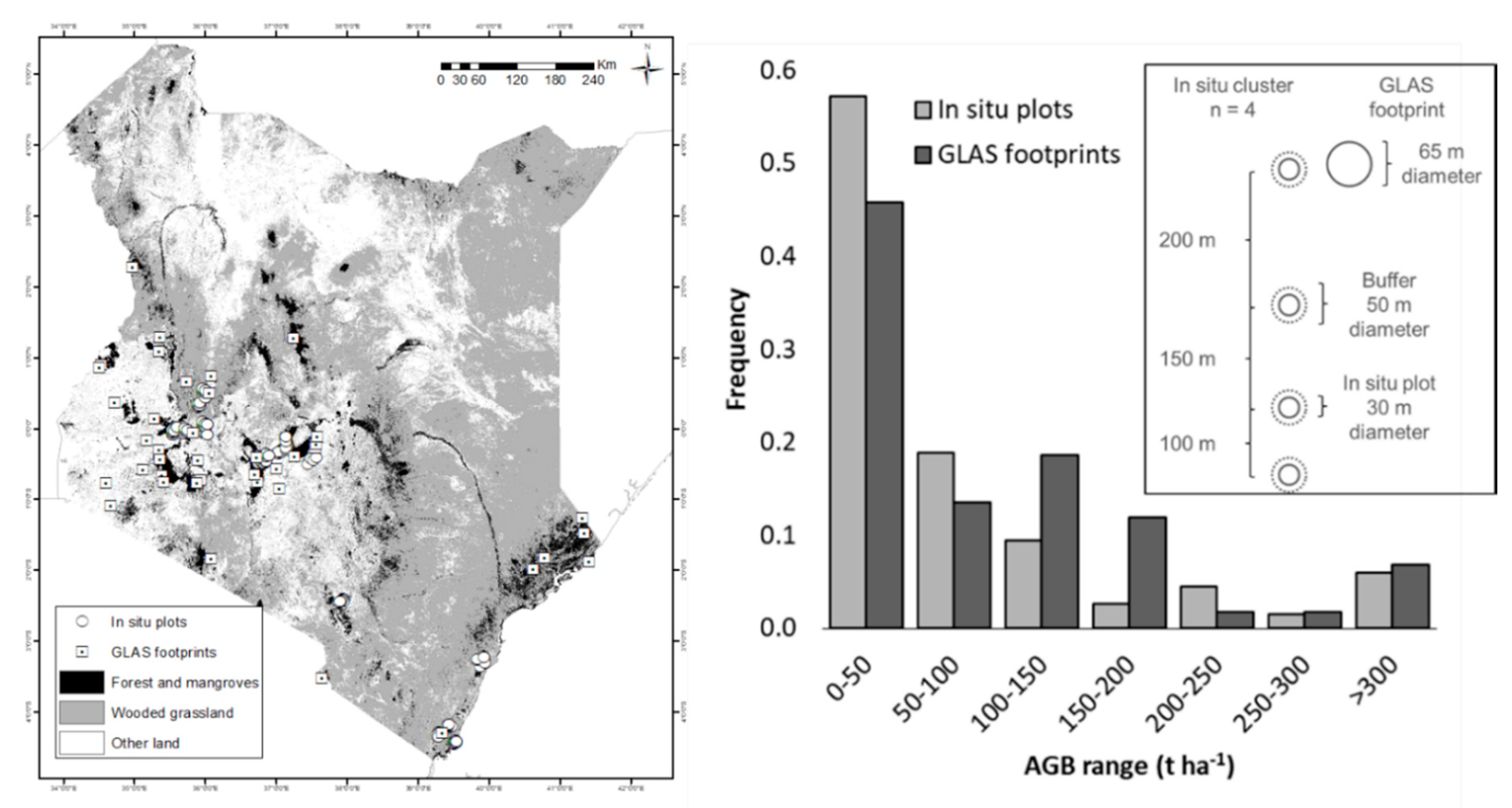
2.1. Reference Datasets

In situ forest inventory plots were established following a stratified random sampling across four forest ecosystems (Montane and Western Rain forest, Dryland Forest, Coastal and Mangrove and the Plantation Forest) and three canopy density classes (dense, moderate and open) across Kenya [43,44]. The data was collected by the Kenya Forest Service (KFS) during a pilot forest inventory taken between 2014 and 2016. Species identification of trees, bamboos and lianas, as well as non-destructive measurements of diameter at breast height and total height were acquired within each plot [43]. Approximately 61% of the plots were in forest and woodlands, 22% in dryland forest and wooded grasslands and the remaining 17% in mangroves and other coastal forest. This dataset consisted of 266 circular plots 30 m diameter (0.07 ha). We used all these plots for training and validation of the AGB map. Plots were sometimes gathered in 4-plot clusters (0.28 ha per cluster) where plots were set in a straight line and separated by different distances (Figure 1). This sampling design allowed us to validate the AGB map at the cluster level as well (0.28 ha). Some plots stood alone or were in clusters containing fewer than 4 plots for a variety of reasons (e.g., no access due to private property). Only clusters with 4 plots (i.e., 40 clusters) were considered for validation.
Due to the small number of plots available, LiDAR footprints from the Geoscience Laser Altimeter System (GLAS) onboard the ICESat satellite acquired between 2004 and 2008 were also used for validation. The footprints sampled over forested areas were acquired from a spatially balanced sample at the national level [45,46]. GLAS data consist of full waveform LiDAR acquisitions, with each footprint having a diameter of approximately 65 m (0.33 ha) (Figure 1). The canopy height was estimated for all LiDAR footprints using the full waveform parameters and the method proposed by Lefsky [47], while aboveground woody biomass (AGB) was derived using the allometric model proposed for Africa by Saatchi et al. [22]. For Kenya, 40 footprints were available, which we could increase to 64 by including footprints in close proximity from Tanzania, Somalia and Uganda. Due to the temporal discrepancy between the GLAS LiDAR footprints (2004–2008) and this study (2014 ± 1), we screened the footprint locations for disturbances in the dates between that time interval using the Hansen et al. [3] forest loss product. From the final selection of footprints, 5 were discarded as forest loss was detected.
A dataset consisting of 500 polygons (60 m × 60 m) depicting stable classes according to the Kenya land cover map 2014 [48], i.e., stable forest (SF), stable other vegetation (SOV), stable other land (SOL) and stable water (SW), together with forest loss (Floss) during the 2014–2017 period, was generated by means of stratified random sampling and the use of time series of very high resolution (VHR) imagery available through Google Earth Pro. Each sample was visually interpreted and labelled. The dataset was then randomly divided into training and validation subsets (70% and 30%, respectively) and used to map these classes over the study period (2014–2017).

2.2. Landsat 8 Operational Land Imager (OLI)

Landsat 8 OLI surface reflectance Tier 1 imagery from the U.S. Geological Survey (USGS) acquired between 2014 and 2017 over Kenya was used to produce cloud-free annual 30 m resolution composites. Landsat 8 OLI data are atmospherically corrected using the Land Surface Reflectance Code (LaSRC) [49] by the USGS and includes a cloud, shadow, water and snow mask derived by the C Function of Mask (CFMASK) algorithm. We only retained bands 3 (Green; 0.533–0.590 μm), 4 (Red; 0.636–0.673 μm), 5 (Near Infrared, NIR; 0.851–0.879 μm), 6 (Shortwave Infrared 1, SWIR1; 1.566–1.651 μm) and 7 (Shortwave Infrared 2, SWIR2; 2.107–2.294 μm). In addition, a set of spectral indices was included: normalised difference vegetation index (NDVI) [50], soil adjusted vegetation index (SAVI) [51], enhanced vegetation index (EVI) [52], normalised difference moisture index (NDMI) [53] and normalised burn ratio (NBR) [54]. For each annual composite image, we selected for each pixel the median value of all observations with low confidence cloud and low confidence cirrus over land, water and snow/ice. These annual composites are the basis for mapping stable classes and detecting forest loss in the 2014–2017 period. Additionally, a median value composite and vegetation indices were generated using the same procedure with data from 2014 ± 1 yr. Imagery from 3 years (i.e., 3340 scenes) was needed to generate a completely cloud-free composite for the whole of Kenya. This composite was used as input for generating the AGBC map.

2.3. Advanced Land Observing Satellite (ALOS) Phased Array Type L-Band Synthetic Aperture Radar (PALSAR)

The L-band PALSAR (2007–2010) and PALSAR-2 (2015–2017) mosaics produced and distributed by JAXA under the ALOS Kyoto and Carbon Initiative [55] consist of dual-polarisation, pre-processed, incidence-angle corrected radar backscatter expressed as γ0 in dB as follows:
γ 0 = 10 × l o g 10 ( D N ) 2 + C F
where DN is the pixel digital number and CF is the calibration factor (−83.0 dB).
The pre-processing of these data products [55] involves calibration, multi-looking (16 looks), projection, orthorectification and slope correction using the Shuttle Radar Topography Mission (SRTM) Digital Elevation Model (DEM) data, along with a de-striping process [56]. We applied a multi-channel filter [57] on the annual mosaics (2007–2010, and 2015–2017) with a 5 × 5 window to reduce speckle. After performing the filtering, only the 2015 mosaic was used. The registration of PALSAR/PALSAR-2 mosaics showed more than 80 m displacement in some regions. This error comes in the processing of the mosaics, resulting sometimes in shifts and sometimes in deformation ([58], personal communication to K&C team). Therefore, an additional fine co-registration of the 2015 PALSAR-2 mosaic was performed using a Sentinel-1 mosaic as reference. This was preferred over a SAR-to-optical approach because of the different viewing geometry of optical and SAR images, which can lead to inaccurate co-registration. In addition to both backscatter polarisations ( γ H H 0 and γ H V 0 ), we calculated the cross-polarisation ratio ( C p R = γ H V 0 / γ H H 0 ) and the Radar Forest Degradation Index ( R F D I = γ H H 0 γ H V 0 / γ H H 0 + γ H V 0 ) [59].

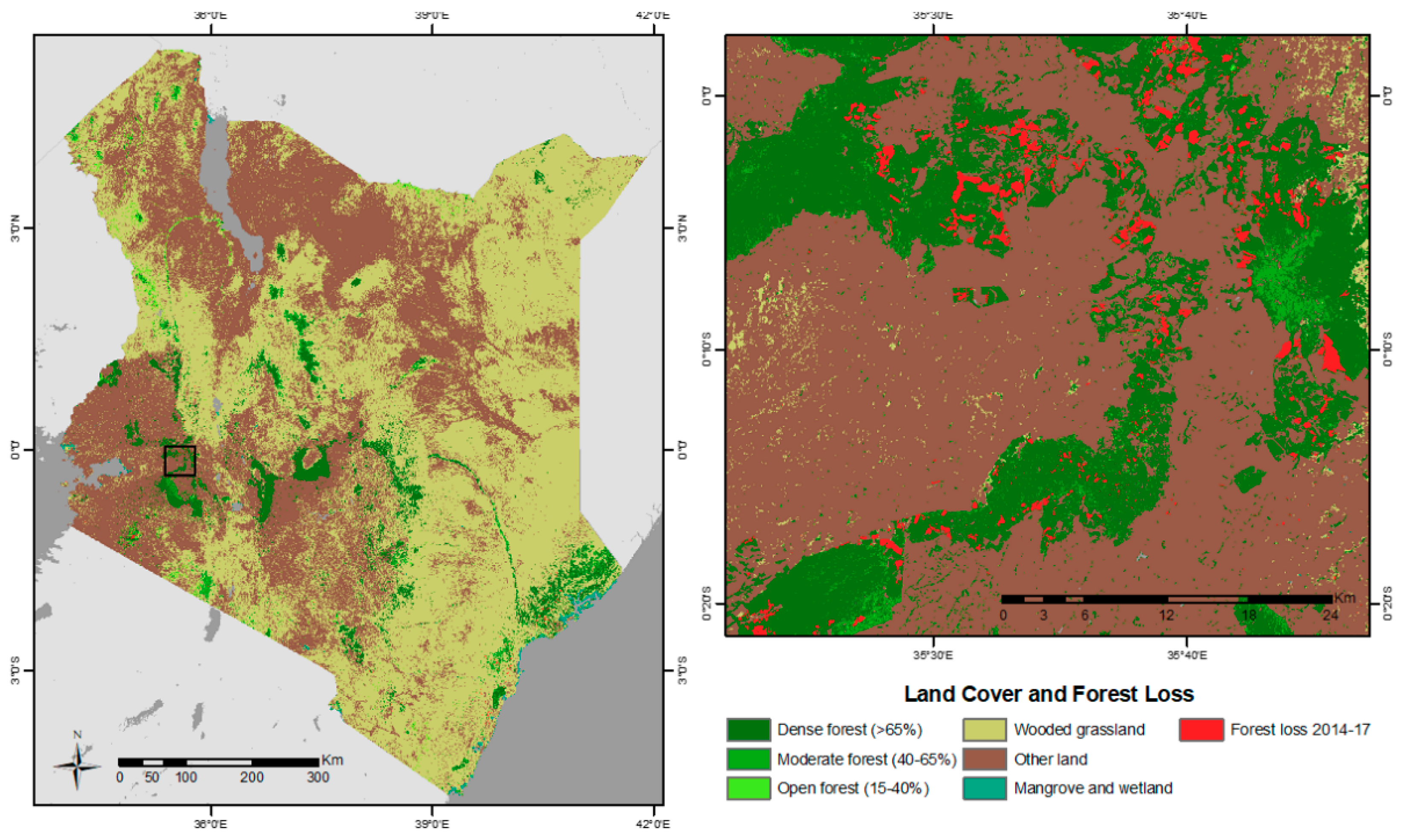
2.4. Land Cover Data

The Government of Kenya initiated a process for developing a system for the estimation of land-based emissions in Kenya [4], and among the products developed were the national land cover classification maps [48] based on IPCC guidelines [60]. The Kenya land cover map is a 10-class map with 30 m spatial resolution developed using Landsat imagery. The classes are dense forest (canopy cover > 65%), moderate forest (canopy cover 40–65%), open forest (canopy cover 15–40%), wooded grassland, open grassland, perennial cropland, annual cropland, mangroves and vegetated wetlands, open water and other land. The Kenya land cover product for the year 2014, in combination with the JRC Global Surface Water product [61], was used to constrain the AGBC retrievals to only woody vegetation classes: dense forest, moderate forest, open forest, wooded grassland and mangroves and vegetated wetland. As previously mentioned, the land cover map was also used to guide the stratified selection of reference observations of stable land cover classes in the 2014–2017 period.

2.5. Global Forest Change

The Global Forest Change (GFC) dataset v 1.6 [3] is a 30 m Landsat-based product that depicts tree canopy cover for the year 2000, annual forest cover loss, and total forest cover gain for the period of 2000–2018. The tree canopy cover 2000 and the loss/gain data from the 2000–2014 period were used to generate a 2014 tree canopy cover product for Kenya used as input to generate the AGBC map. Additionally, the validation subset was used to evaluate the accuracy of the GFC annual forest loss for the period 2014–2017 over Kenya in order to assess its value in constraining the CARDAMOM analysis to undisturbed woody classes only (see Section 3.4 for details).

2.6. Leaf Area Index

The Copernicus Global Land Service (CGLS) Collection 300 m Leaf Area Index (LAI) Version 1 dataset was used as the input for the CARDAMOM analysis. This dataset is based on the daily top-of-atmosphere reflectance measured in the blue, red and near infrared channels [62,63]. These were transformed into estimates of LAI using a neural network in an approach similar to Baret et al. [64] and Camacho et al. [65]. The daily estimates were smoothed, gap-filled and composited over 10-day periods starting in January 2014. The uncertainty of the composited product is reported as its root-mean-squared difference (RMSD) from daily estimates in the compositing period. The data were taken from the CGLS online portal (http://land.copernicus.eu/).

2.7. Burned Area and Soil Data
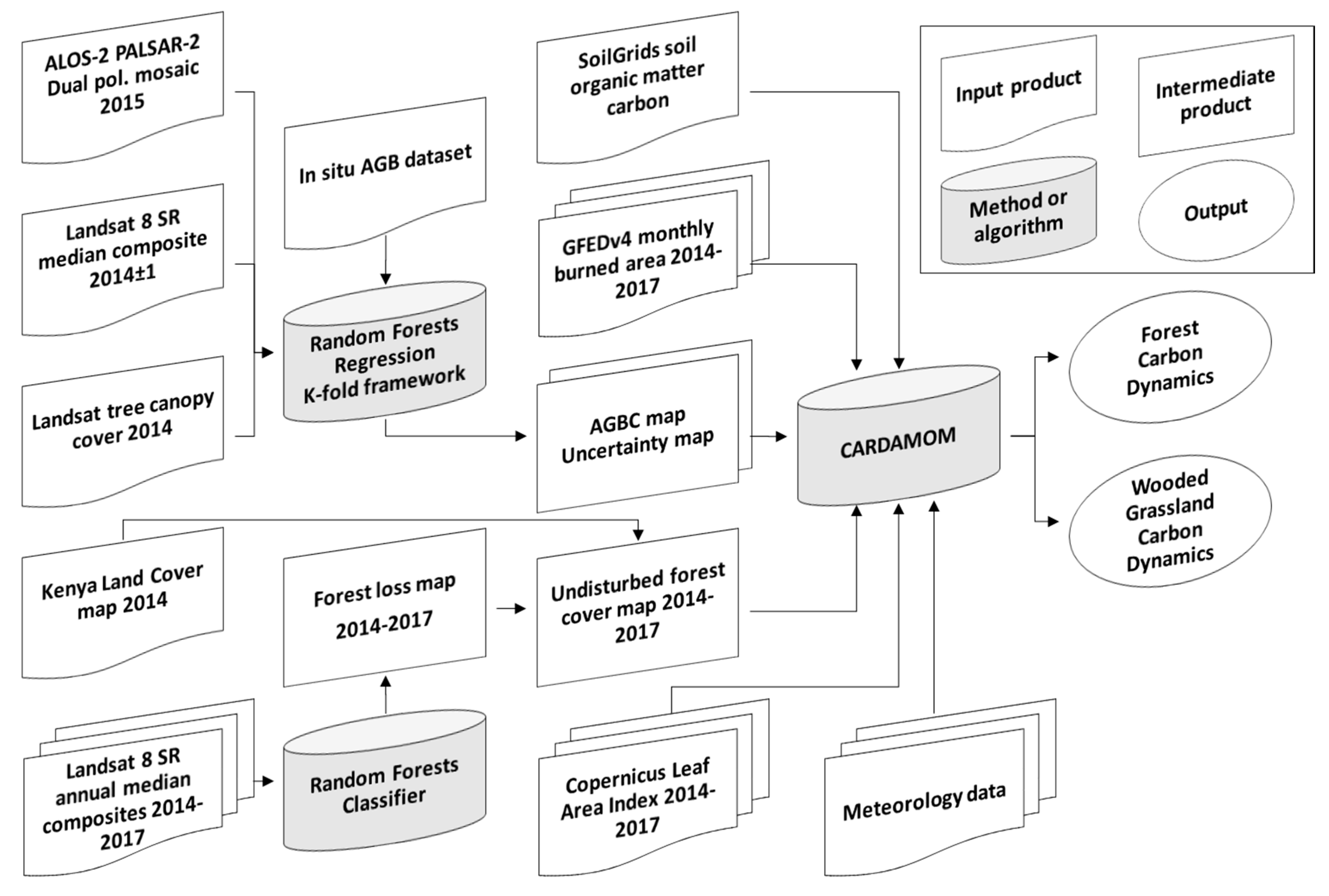
The Global Fire Emissions Database version 4 (GFEDv4) was used to provide time series information on the burned area at monthly time steps and 0.25° × 0.25° spatial resolution over Kenya [66]. This was used to impose observed fire disturbance on the CARDAMOM analyses. CARDAMOM also requires a prior estimate of the magnitude of the organic soil carbon stock, extracted from the SoilGrids (250 m × 250 m) product [67]. SoilGrids was chosen over other products due to a recent review of global soil maps against independent data indicating a greater degree of skill in the SoilGrids (see https://www.soil-journal.net/5/137/2019/for details). For details on the data aggregation, see Section 3.4.

3. Methods

The methodology adopted here has the following components: (i) in situ AGB estimation using pantropical allometries, (ii) AGBC map production, (iii) mapping stable classes and forest loss and (iv) carbon cycle analysis using a model-data fusion framework (Figure 2).
We used a non-parametric machine learning random forest algorithm [68] to perform regression and supervised image classification. Random forests (RF) have been used extensively to retrieve biophysical parameters and land cover from remote sensing data [19,69,70,71]. RF is built as an ensemble of binary decision trees, where each tree is fitted to a bootstrap sample of the training dataset (with replacement) and the final prediction is generated as the average of all the estimates (for regression) or by majority vote (for classification). The observations not selected for fitting a RF model (the out-of-bag (OOB) sample) are combined to give the overall estimate of error. A sensitivity analysis was carried out to find the combination of hyper-parameters generating the lowest OOB error.

3.1. AGB Estimation Using Allometric Models

The AGB for in situ plots was estimated using pantropical tree allometries [72] with diameter at breast height, tree height and wood specific gravity as input variables (Equation (A1)) for all the trees within each plot. The AGB of bamboos was estimated using Muchiri and Muga [73] allometries (Equations (A2) and (A3)), while the AGB of lianas was estimated using the volume of the equivalent cylinder and the mean wood density of 0.6 g m−3 [74]. For the LiDAR footprints, AGB was estimated using the Saatchi et al. [22] footprint allometric model for sub-Saharan Africa, which used GLAS-derived canopy height as predictor variable (Equation (A4)). The histograms of AGB values from both datasets were similar (Figure 1), with an average AGB from the in situ plots and GLAS dataset of 90.7 t ha−1 and 97.6 t ha−1 respectively.

3.2. Biomass and Carbon Mapping

As the in situ plots were relatively small (30 m diameter) and geographical coordinates obtained with a GPS under a forest canopy can have substantial geolocation error (5–10 m) [43], the AGB field data may not correspond exactly to the overlapping pixel values at a given location. Therefore, we added a 10 m buffer around the plot boundaries to obtain a representative 50 m diameter circular area (Figure 1). We then extracted the average value of all the EO pixels from the different predictors overlapping those areas to train the supervised regression. This had the aim of averaging out any geolocation errors in the plots.
The AGB map was generated by combining the in situ AGB measurements with L-band SAR ALOS-2 PALSAR-2 ( γ H V 0 , γ H H 0 , RFDI and CpR), multispectral Landsat data (Green, Red, Near infrared, both Shortwave infrared bands, NDVI, NBR, NBR2, NDMI and SAVI) and a Landsat tree canopy cover product, and running RF within a stratified k-fold cross-validation framework. This framework was designed to make the best use of the limited data available for training, to validate the map and, at the same time, to estimate our prediction error at pixel level based on the standard deviation of the k predictions performed by the models calibrated with different groups of data (see Appendix A).
The Kenya land cover product [48] and JRC Global Surface Water product [61] were used to constrain the predictions to only forests, wooded grasslands and savannahs, mangroves and vegetated wetlands, so water, croplands, open grasslands and bare land classes were set to zero AGB. The AGB and SD maps in units of t ha−1 were then converted to AGBC units (i.e., t C ha−1) by using a 0.47 conversion ratio [75]. We also estimated the belowground biomass carbon (BGBC), i.e., the biomass carbon of live roots, using a root-shoot ratio of 0.24 [75].
For accuracy assessment of the AGBC map we quantified the difference between our map and the reference data using the mean bias difference (MBD), the mean absolute difference (MAD), the root mean square difference (RMSD) and the relative squared difference (RSD) (Appendix A). We also performed an accuracy assessment stratified by the AGBC range as seen in Rodríguez-Veiga et al. [14] to evaluate random errors and biases using the Coefficient of Variation of the bias (CVbias) (Appendix A).

3.3. Forest Loss Mapping

The previously described 500 squares of 60 m × 60 m from the training dataset depicting stable classes (SF, SOV, SOL and SW; according to the Kenya land cover map—see Section 2.1) and forest loss were used to extract the average value from each Landsat 8 OLI band and derive spectral indices. A RF classifier was then used to perform supervised classification on a 70% random sample of that dataset (n = 350). This map was validated using the validation subset (n = 150). The validation results are reported using the testing subset to generate the corresponding confusion matrix, which was corrected using the mapped area of each class according to Olofsson et al. [76].
RF gives the proportion of votes in each class on a pixel-by-pixel basis, which can be viewed as an indicator of classification confidence. A likelihood scale can then be defined according to these values using a similar approach to that developed by IPCC (2010). The likelihood of an outcome could be defined as “unlikely” (probability < 0.33), “about as likely as not” (probability = 0.33–0.66) and “likely” (probability > 0.66). We applied these intervals to the predictions from the RF model and generated three levels of likelihood per class. We then used the “likely” (probability > 0.66) Floss class to update the forest cover area to focus only on undisturbed forest during the study period.

3.4. Carbon Cycle Analyses: CARbon DAta MOdel fraMework (CARDAMOM)

We used the CARDAMOM [38,40,41] model-data fusion framework to analyse the terrestrial carbon cycle in Kenya at 0.25° spatial resolution and monthly time step. CARDAMOM combines the Data Assimilation Linked Ecosystem Carbon version 2 (DALEC2), which is an intermediate complexity model of the terrestrial carbon cycle (Bloom and Williams [39]), with biophysical observations and their uncertainties, plus meteorological information. Ecological and dynamic constraints (EDCs) are used in CARDAMOM to ensure sensible parameter searches within a Bayesian framework using an Adaptive Proposal-Markov Chain Monte Carlo (AP-MCMC). This process retrieves ensembles of location-specific model parameters, providing probabilistic estimates of fluxes and pools of C over the analysis period. The EDCs ensure that carbon cycle dynamics and trait retrieval are consistent with ecological theory (e.g., ensuring litter turnover is faster than that of soil organic matter), as described in Bloom and Williams [39]. DALEC simulates photosynthesis, respiration, the allocation of photosynthate to foliar, root and wood pools, their turnover and the subsequent decomposition in the litter and soil carbon pools.
CARDAMOM was used to estimate the carbon cycle of undisturbed Kenyan forests and wooded grasslands for 2014–2017 under meteorology extracted from ERA-Interim re-analysis climate data [77]. Fire was imposed using GFEDv4 (see Section 2.7) following the approach of Exbrayat et al. (2018). Time series of LAI from the Copernicus Land Monitoring Service [64] were assimilated into CARDAMOM to constrain canopy phenology and productivity, while the maps of AGBC (this study) and soil organic matter carbon (SoilGrids; see Section 2.7) constrained the initial status of the corresponding carbon pools.
The CARDAMOM analysis was conducted at 0.25° × 0.25° resolution as this was the resolution of the coarsest dataset used (GFEDv4). However, many of the other observational constraints have finer spatial resolutions. Using the map of undisturbed forest (this study) we resampled the AGBC estimate, LAI time series and soil organic matter information from their native resolution to 0.25° following [78]. Each 0.25° grid cell was analysed by CARDAMOM using the average status of the undisturbed forest within that pixel after removing contamination by other land cover types. Overall, a total of 761 grid cells were simulated to represent the mean undisturbed forest state. To ensure convergence, CARDAMOM’s AP-MCMC procedure was repeated three times at each location for 100 million iterations. Convergence was then tested using the Gelman–Rubin convergence criterion. Grid cells which did not converge across the three repeated analyses were re-run. The results presented here were derived by subsampling 250 parameter sets from the second half of each chain. Pixel level uncertainties are estimated directly from the probability density function estimated from the ensemble of simulations from the parameter sub-sample.
Estimates of the following land-atmosphere fluxes are reported in Section 4: gross primary productivity (GPP), autotrophic respiration (Ra), net primary productivity (NPP = GPP − Ra), heterotrophic respiration (Rh), net ecosystem exchange (NEE = −NPP + Rh) and net biome exchange (NBE = NEE + Fire). For NEE and NBE, negative values indicate a net C uptake from the atmosphere. CARDAMOM also generates estimates of ecologically important information on the partitioning of photosynthate allocated to plant tissues and their mean residence times, as well as carbon cycling.

4. Results

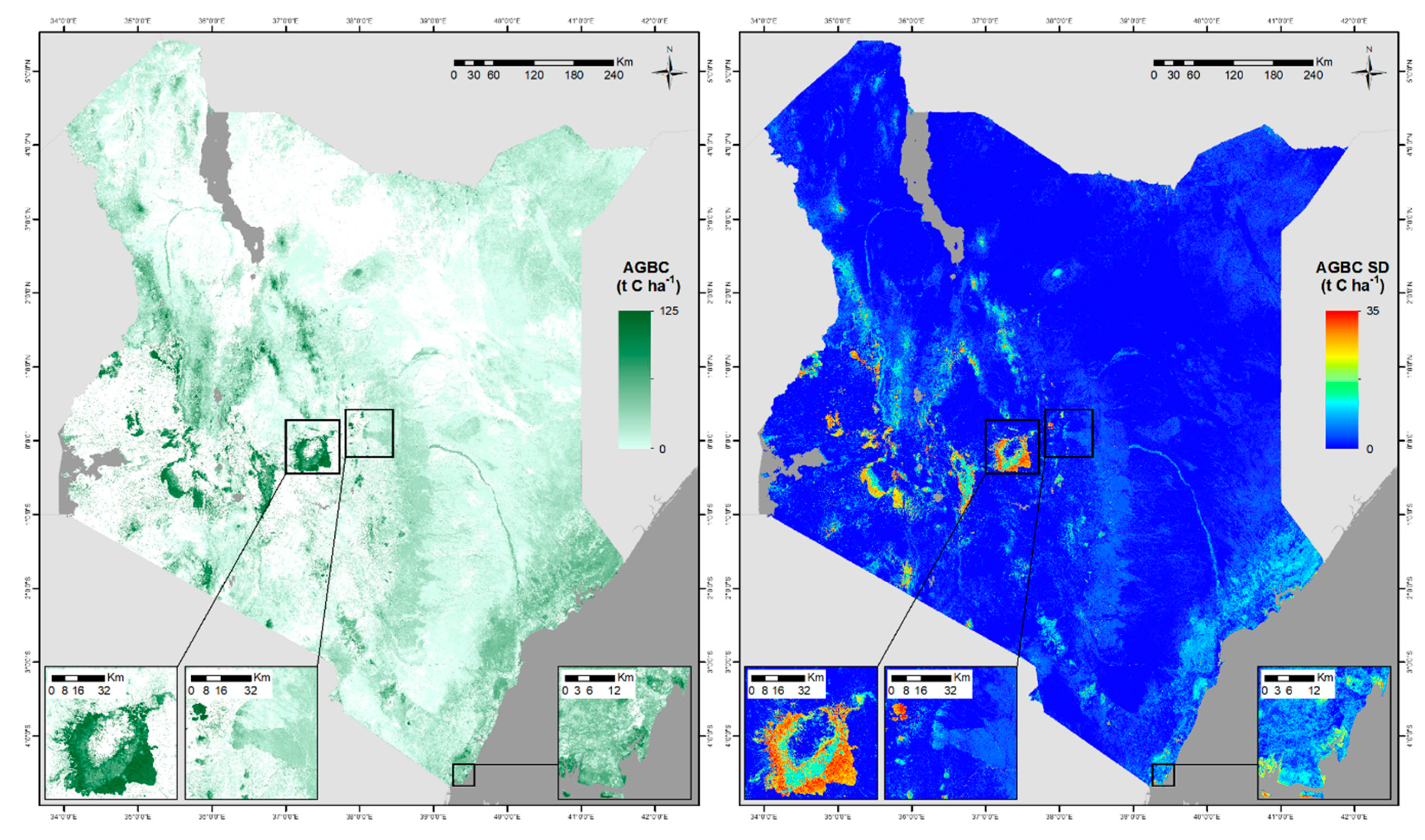
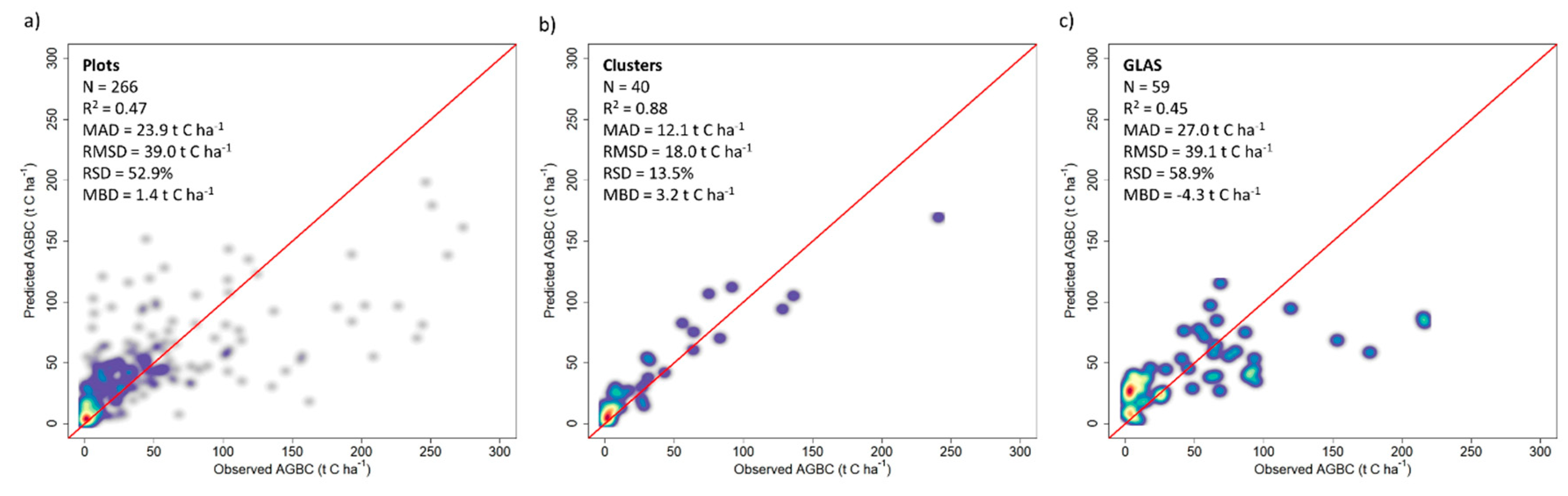
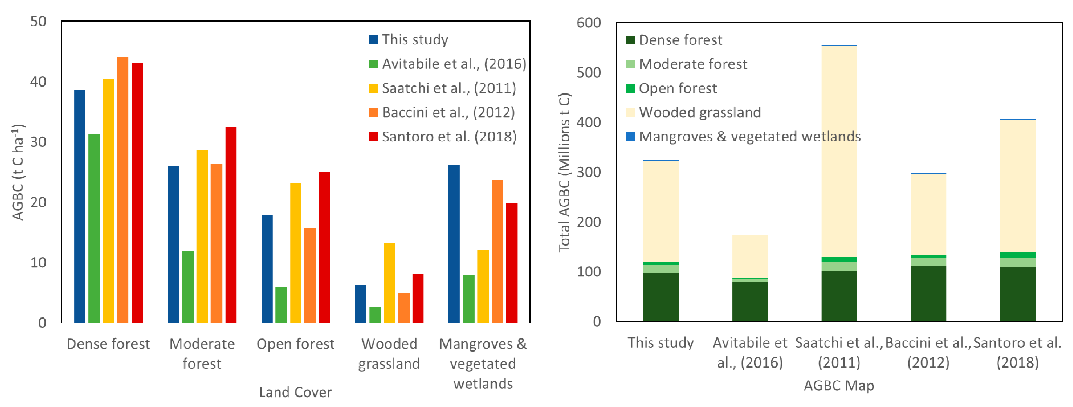
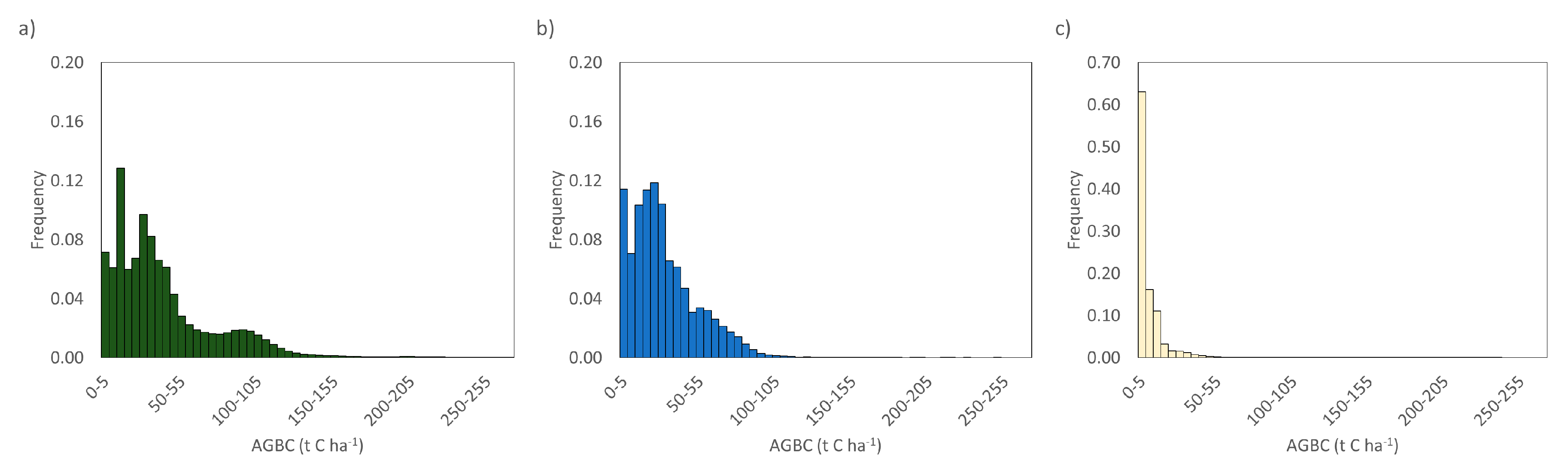
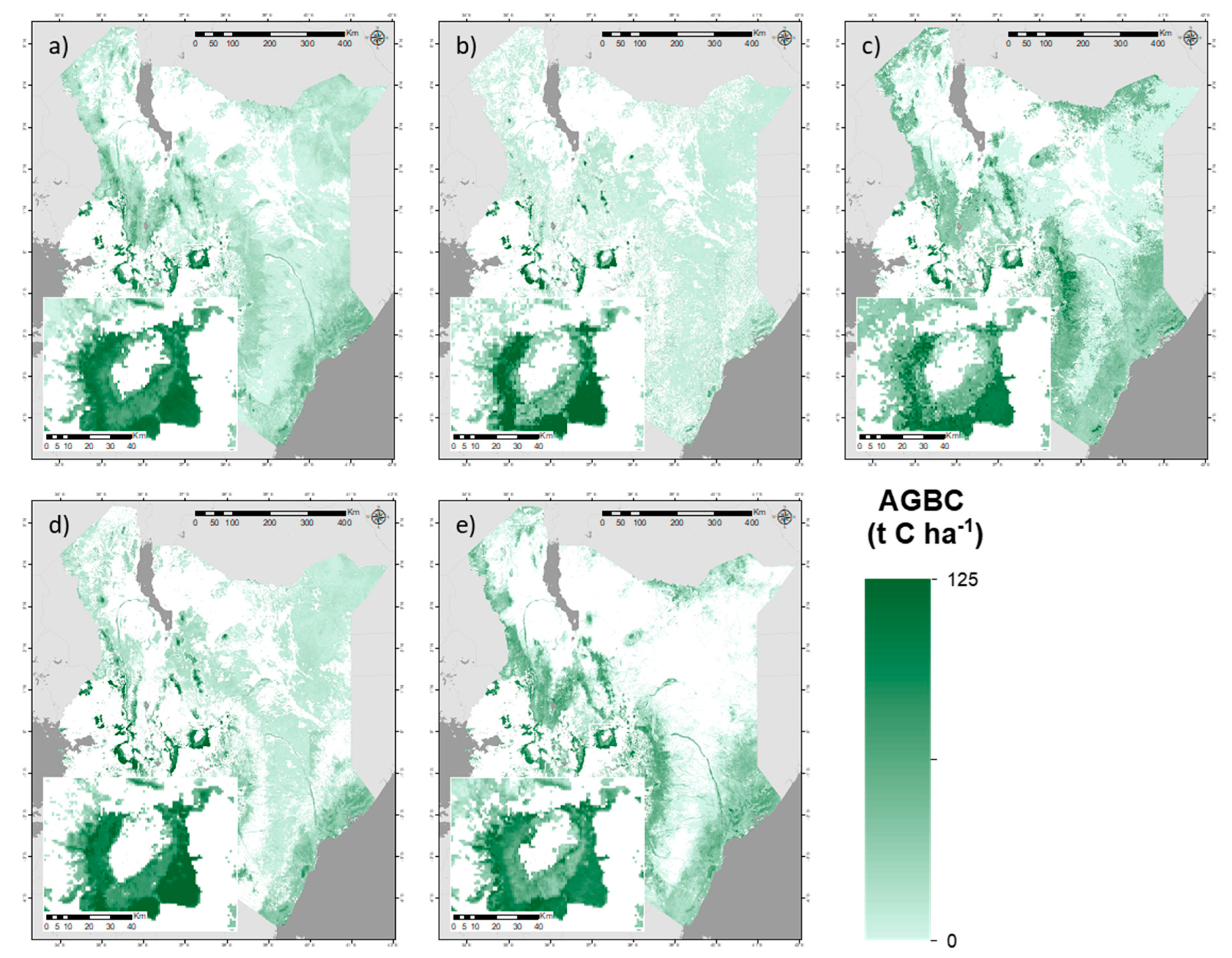
4.1. Biomass Carbon Stocks

The AGBC map for Kenya and its associated uncertainty map (Figure 3) shows a concentration of AGBC in the western mountainous areas of the country and in the eastern coastal region.
The accuracy of the AGBC map was assessed using in situ plots, plot clusters and GLAS LiDAR footprints (Figure 4). The assessments at plot and cluster level are the result of the k-fold cross-validation framework, whereas the GLAS LiDAR footprints give an additional independent validation. The accuracy assessment at plot level showed a coefficient of determination (R2) of 0.47, RMSD of 39.0 t C h−1, RSD of 52.9%, and MBD in the overall mean of 1.4 t C ha−1. At cluster level, R2 was 0.88, the RMSD was 18.0 t C ha−1, the RSD was 13.5% and the MBD was 3.2 t C ha−1. Validation with the GLAS footprint data gave similar results, with R2 of 0.45, RMSD of 39.1 t C ha−1 and MBD of the mean of −4.3 t C ha−1.
The error analysis indicated that random error, as measured by the CVbias, was dominant in the low and middle AGBC ranges predicted by the map for plots and clusters. In the case of plot and GLAS level assessments, bias dominated the error in ranges above 75 t C ha−1 for GLAS and 135 t C ha−1 for plots, which resulted in an underestimation of AGBC (Figure 4 and Table A1). However, this effect is reduced when assessing the errors using larger units (i.e., clusters).
Using the AGBC and the uncertainty map, we computed an average AGBC of 36.69 ± 17.04 t C ha−1 for forests (open to dense forests and mangroves) and 6.01 ± 2.98 t C ha−1 for wooded grasslands. The highest AGBC densities estimated by the map in Kenya are in the dense forest areas, with values up to 250.50 t C ha−1. The lowest AGBC values are found in the wooded grassland areas. Kenya is dominated by arid and semi-arid conditions, leading to a dominance of low AGBC densities (i.e., wooded grassland, Figure A1). However, the large area covered by wooded grassland means that we estimate ~59% of Kenya’s total AGBC stocks are found there.
The total AGBC stocks for the forests and wooded grasslands in Kenya was estimated to be 339.20 Mt C with a coefficient of variation at national level of <1%. Stratifying by cover type, the total AGBC stock in forests (open to dense forests and mangroves) was 140.70 Mt C, and in wooded grasslands 198.50 Mt C, representing 41% and 59% of the total stocks respectively. The total BGBC was estimated as 81.41 Mt C, resulting in a total biomass carbon stock of 420.61 Mt C.
The AGBC map derived by this study was compared in terms of accuracy and carbon stocks to previous global and pan-tropical studies from Avitabile et al. [24], Saatchi et al. [22], Baccini et al. [23] and Santoro et al. [79] over Kenya at 1 km spatial resolution (Figure A2). These products correspond to different years between 2000 and 2010, while our map corresponds to 2014. We used the GLAS footprints and the clusters to assess the accuracy of these products. We made sure these were not affected by forest disturbances between 2000 and 2015, according to Hansen et al. [3]. This study showed higher accuracy and lower errors than any other product over Kenya (Table A2).
In terms of carbon stocks, Saatchi et al. [22] calculated almost twice the amount calculated by this study or by Baccini et al. [23] for Kenya, and almost three times the stock estimated by Avitabile et al. [24]. Dense, moderate and open forest areas showed similar AGBC values in all the studies, except that of Avitabile et al. [24] with lower AGBC values for all vegetation types (Figure 5). The biggest disagreements between the maps occur for wooded grasslands and mangroves and vegetated wetlands (Figure 5). Each of the AGBC maps indicates that wooded grassland has the largest total AGBC stocks, ranging from 48% to 76% of the total AGBC stock for the country (Figure 5).

4.2. Deforestation and Carbon Loss

The accuracy assessment of the “likely” forest loss class refers to the testing subset and is given as proportions, following Olofsson et al. [76]. Two products were validated using this subset: (i) the globally calibrated forest loss product for 2014–2017 from the GFC dataset [3]; (ii) the locally calibrated forest loss map generated in this study for the 2014–2017 period.
Our locally calibrated undisturbed land cover and forest loss product for the 2014–2017 period in Kenya (Figure 6) showed an overall accuracy of 0.92 and κ of 0.83. The commission error for this forest loss product was estimated at 3%, while the omission error was 0%. For comparison, the globally calibrated GFC forest loss dataset for the 2014–2017 period in Kenya gave a commission error of 0%, and a much higher omission error of 99%, for an overall accuracy of 0.89 and κ of 0.01 (Table A3 and Table A4).
As our locally calibrated forest loss product gave much higher accuracy, it was used for the subsequent analysis. The total forest loss calculated using this dataset for the 2014–2017 period in Kenya was estimated as 30,802 ha (deforestation rate of 10,267 ha yr−1), of which 87% occurred in dense forests (Table 1).
These figures change if wooded grassland is included in the calculation. Then, the total loss would be 43,736 ha (14,579 ha yr−1), with 61% corresponding to dense forest and 30% to wooded grassland.
The combination of the forest loss product with the AGBC map allows us to estimate the AGBC loss rates due to deforestation for the 2014–2017 period (Table 1). In this period, Kenyan forests lost approximately 2.09 Mt C, with an annual loss rate of approximately 0.70 Mt C yr−1, while approximately 0.29 Mt C (0.10 Mt C yr−1) was lost from wooded grassland due to deforestation. The deforestation rate of wooded grasslands was half that of dense forest, but five times more AGBC was lost in the latter. The CV for the total AGBC losses for all forest types was below 1%.

4.3. Ecosystem Carbon Cycling Properties and Dynamics

CARDAMOM accurately simulated the time series of observed LAI and single estimates of AGBC and soil carbon used to constrain its initial conditions (R2 > 0.95 and mean absolute error <10%; Figure A3). Consistent with the AGBC mapping, CARDAMOM estimated that ecosystem productivity (GPP) and growth (NPP) are ~2.5 times greater per hectare for forest ecosystems than for wooded grasslands. However, the more extensive wooded grasslands are overall three times more productive than the forest area at the national scale (Table 2). Carbon losses from both forests and wooded grasslands are dominated by respiration, with fire losses estimated to represent only ~1% of the net biome exchange. Respiration has a similar magnitude from autotrophs and heterotrophs. Given the currently assimilated information, the analysis cannot confidently identify either forest or wooded grassland as a net source or sink of carbon for the analysis period (Table 2). The mean wood stock estimates in 2014 for forests is more than 4 times larger than in wooded grassland. Similarly, the mean magnitude of NPP allocated to wood is ~3 times larger in forests than wooded grassland, while the residence time of wood is ~70% longer in forests than in wooded grassland (Table 3).

5. Discussion

In this study we have combined field inventory and EO information within a machine learning approach to create Kenya-wide improved estimates of AGBC (Figure 3, Figure 4 and Figure 5), forest cover loss (Figure 6, Table 1) and their uncertainties. These and other data have then been used to constrain a process-oriented model of the terrestrial carbon cycle to improve our understanding of the properties and carbon cycling of the Kenyan ecosystem (Table 2 and Table 3).

5.1. Biomass Carbon Stocks

The total AGBC stock estimated for Kenya is 339.20 Mt C. The coefficient of variation for AGBC at national level was calculated to be <1%, which agrees with Saatchi et al. [22]. However, this result must be treated with caution, as the CV of a sum of measurements can be made arbitrarily small by adding more measurements/pixels (i.e., increasing the area of interest). This is because the precision of the estimated total AGBC improves as the number of pixels increases (see Equations (A8) and (A9)), but the accuracy of the estimate may increase or decrease as new measurements are added if there are systematic biases in the measurements. The potential error depends on how bias depends on true AGBC and the histogram of the true AGBC for the measurements being summed.
Previous EO-based pantropical and global maps correspond to different time-periods and used different reference datasets and methods. These studies have estimated Kenya’s biomass carbon stocks to be 174–556 Mt C, a range encompassing the estimate from this study [21,22,23,24]. However, all the studies give an AGBC stock that is a lot smaller than the 694 Mt C reported in the Forest Resource Assessment (FRA) [75]. The discrepancies between this study and the abovementioned EO-orientated studies is due to the AGBC stocks estimated for wooded grasslands (Figure 5). In the studies, the forest AGBC stock ranges from 88.82 Mt C to 139.21 Mt C, whereas the AGBC from wooded grasslands presents a wider range from 84.22 Mt C to 424.95 Mt C. The lowest estimate for wooded grassland comes from Avitabile et al. [24]; this is not surprising as this used the GLC2000 map [80] as a forest mask, which excluded a large proportion of wooded grassland and other vegetation types from their estimation, as seen in Figure 5. These large differences at national level, in the order of hundreds Mt C, cannot be explained by inter-annual AGBC variation. Nevertheless, all studies suggest that the largest pool of AGBC in Kenya is in wooded grasslands.
However, due to their low tree density wooded grasslands are not considered forest under the Kenyan forest definition and are therefore not included within the framework of national and international mechanisms aiming to protect carbon stocks, such as REDD+. This is an indication that the role of wooded grasslands in the C cycle is not fully understood and that this role is undervalued, as recently stressed by McNicol et al. [31], who for the first time identified: (i) degradation as the main driver of C loss in the highly dynamic southern African savannahs and woodlands; and (ii) the importance played by extensive regrowth, making this region a significant sink of carbon. Even mechanisms such as the Bonn Challenge, which aims to reforest 150 Mha by 2030, include some wooded grasslands and savannahs as targets for its afforestation agenda [81], implying that these ecosystems need to be converted to forest, thereby underestimating not only their climate mitigation capacity in their own right but also their ecological importance. Furthermore, fluxes from degradation and regrowth, including recent reforestation efforts made by the government of Kenya to increase the forest cover of the country to 10% of the national territory by 2022 [2], are unaccounted for.

5.2. Deforestation and Carbon Loss

We compared the accuracy of the locally calibrated forest loss product (Figure 6) generated in this study with a globally calibrated forest loss product (GFC) [3] for Kenya. The GFC product does not perform well for Kenyan forests and has a large omission error, indicating that it does not detect most of the deforestation occurring in the country (Table A4). This has implications when calculating the overall carbon budget for Kenya. As Kenya’s carbon stocks are relatively low, a miscalculation of the deforestation might change the estimate from a net C source to net C sink and vice versa. Likewise, Milodowski et al. [29] found that the GFC provides robust estimates of forest loss for large-scale deforestation areas, but has serious problems detecting small-scale disturbances (<2 ha).
The estimated deforestation rates in Kenya between 1990 and 2015, as reported by the Food and Agriculture Organization (FAO), are approximately 12,400 ha yr−1 [1], which roughly agrees with the average deforestation rate of 10,459 ha yr−1 (14,265 ha yr−1 if wooded grassland is included) reported in this study for the 2014–2017 period. Based on these deforestation rates we estimated that 2.38 Mt C was lost due to deforestation in that period (annual rate of 794,972 t C yr1).
It should be noted that the deforestation rates reported in this study are only based on forest cover loss, as satellites do not see if regrowth is allowed or there is land cover conversion after forest removal. Additionally, our products do not differentiate harvesting occurring in forest plantations or concessions from illegal logging of protected forests.

5.3. Ecosystem Carbon Cycling Properties and Dynamics

The CARDAMOM analysis emphasises the importance of carbon cycling in wooded grassland ecosystems for Kenya’s overall biosphere carbon balance (Table 2 and Table 3). Wooded grasslands cover approximately 62% of the country while forest only covers approximately 7%, so the national carbon fluxes both into and out of wooded grasslands are much larger (Table 2). Despite their limited tree cover, our analysis indicates that at national scale more carbon is fixed into wood each year in the wooded grasslands than in forests (Table 3). Thus, while forest ecosystems may be more productive per unit area, wooded grasslands must be considered in Kenya’s carbon management strategy. The role of fire within both ecosystems was estimated to be <1% of the net biome exchange of carbon (Table 2). However, this estimate should be treated with caution given the widely reported difficulty in detecting small fires from space, which has led to significant efforts to improve small fire detection in recently released products, e.g., [28].
Given the currently available observational datasets, the remaining uncertainties in net carbon exchange make it impossible to identify either forests or wooded grasslands as net sources or sinks of carbon (Table 2). Large uncertainty in the net carbon balance is expected given the lack of repeat measurements of woody biomass [38] or additional information that constrains the woody residence time and/or net carbon exchange. Future CARDAMOM studies will be able to take advantage of new EO-based estimates of biomass to provide additional constraints, such as the annual assessment of woody biomass and its changes, e.g., ESA Biomass mission e.g., ESA Biomass mission [82]. In the near-term, subsequent studies should investigate the usefulness of assimilating net biome exchange estimates derived from atmospheric inversion analysis [83,84].
The CARDAMOM analysis focuses only on forest and wooded grasslands that were undisturbed between 2014 and 2017 and therefore does not account for degradation, reforestation or afforestation activity which occurred prior to the analysis period or degradation during this period. Additionally, the analysis of vegetation dynamics does not represent the complex dynamics in this ecosystem due to large herbivores, pastoral practices and small-scale fires not detected in the GFEDv4 burned area product.

6. Conclusions

The assessment of forest carbon fluxes at national level requires precise and detailed carbon stock estimations. However, the limited availability of in situ data together with the lack of accurate forest carbon maps with fine enough spatial resolution for Kenya have until recently made this particularly challenging.
The AGBC map and the forest loss products generated by this study are the most accurate and detailed published for Kenya to date, giving estimates for every 30 m pixel along with an estimate of the associated pixel-level uncertainty. They complement other Landsat-based national forest land cover methods, and therefore facilitate national and international reporting on carbon dynamics. The AGBC map quantifies carbon stocks not only for forests but also for wooded grasslands, which are often neglected in this type of analysis. The AGBC and forest loss maps allowed us to produce the most complete analysis of carbon stocks and fluxes for the forests and wooded grasslands in Kenya. This study can therefore be considered a benchmark for studying carbon fluxes at national level.
Our results emphasise the importance of other vegetated ecosystems (i.e., wooded grasslands) besides forests for carbon sequestration, and stresses the importance of considering those in Kenya’s carbon management strategy. Wooded grasslands represent 59% of the AGBC stocks in Kenya due to the large area of this ecosystem type. However, unlike forests, international mechanisms for climate mitigation, such as REDD+, do not recognise the importance of wooded grasslands by providing economic incentives for their preservation and management. Moving from a concept of a discontinuous landscape described by categorical land cover classes to a continuous landscape paradigm describing landscapes through biophysical parameters such as percentage canopy cover will provide a way forward for such international mechanisms.

Author Contributions

Conceptualization, P.R.-V., J.C., T.L.S., J.-F.E., J.N., M.W., and H.B.; methodology, P.R.-V., J.C., T.L.S., S.Q., M.W., and H.B.; validation, P.R.-V., J.C., and T.L.S.; formal analysis, P.R.-V., J.C., T.L.S., and D.N.; data curation, D.N., F.M., P.R.-V., J.C., and T.L.S.; writing—original draft preparation, P.R.-V.; writing—review and editing, P.R.-V., J.C., T.L.S., J.-F.E., J.N., F.M., D.N., S.Q., M.W., and H.B.; visualization, P.R.-V., and T.L.S.; supervision, J.N., S.Q., M.W., and H.B.; funding acquisition, H.B. and M.W. All authors have read and agreed to the published version of the manuscript.

Funding

This research was supported by the Natural Environment Research Council, Agreement PR140015 between NERC and the National Centre for Earth Observation as part of the NCEO Official Development Assistance (ODA) Programme. The research was also supported by the UK Space Agency International Partnerships Programme (IPP) Forests 2020 project, and ESA Biomass Climate Change Initiative (CCI+) project.

Acknowledgments

The authors would like to thank the following organizations for making the data freely available: JAXA, NASA, ESA, USGS, ISRIC, CGLS, ORNL DAAC, Google, and University of Maryland.

Conflicts of Interest

The authors declare no conflict of interest. The funders had no role in the design of the study; in the collection, analyses, or interpretation of data; in the writing of the manuscript, or in the decision to publish the results.

Appendix A. Methods

Appendix A.1. AGB Estimation Using Allometric Models

The allometric model from Chave et al. [72] was used to estimate tree AGB:
A G B = 0.0673 × ( ρ D 2 H ) 0.976
where D is diameter at breast height in cm, H is tree height in m and ρ is wood specific gravity in g cm−3.
The allometries from Muchiri and Muga [73] were used for AGB of bamboos:
A G B = 1.04 + 0.06 × D × ( 1.11 + 0.36 × D 2 )   for   bamboos   with   D   >   3 cm
A G B = 1.04 + 0.06 × D × ( 1.11 + 0.36 × 3.1 2 )   for   bamboos   with   D     3 cm
The volume of the equivalent cylinder and the mean wood density of 0.6 g m−3 [74] was used to estimate the AGB of lianas.
In the case of GLAS LiDAR footprints, AGB was estimated using a footprint level allometric model developed by Saatchi et al. [22] for sub-Saharan Africa including woodland savanna:
A G B = 0.3542 × H L 2.0528
where HL is the basal area weighted canopy height (i.e., Lorey’s height).

Appendix A.2. K-Fold Cross Validation and AGB Error Mapping

The original sample of in situ data was stratified into 3 AGB ranges (high, medium, low) and each range (stratum) was randomly partitioned into k equally sized subsamples (k = 10). Of the k subsamples, a single subsample is retained from each stratum as the validation data for testing the RF model, and the remaining k − 1 subsamples are used as training data. The cross-validation process was then repeated k times (the folds), with each of the k subsamples used exactly once as the validation data. Therefore, all observations were used for both training and validation, and each observation was used for validation exactly once. As a result of this framework, the k AGB maps were generated, from which the mean value of all estimates for each pixel was used as the final AGB retrieval ( A G B ^ ):
A G B ^ = i = 1 k A G B i k
where A G B i is the prediction of each of the k AGB estimates. Accordingly, the standard deviation (SD) of all k AGB estimates is defined as:
ε p r e d i c t i o n = 1 k i = 1 k ( A G B i A G B ) ^ 2
The total SD ( ε A G B ) for our final retrieval ( A G B ^ ) is then propagated as explained in Rodriguez-Veiga et al. [15], where:
ε A G B = ( ε m e a s u r e m e n t 2 + ε a l l o m e t r y 2 + ε s a m p l i n g 2 + ε p r e d i c t i o n 2 ) 1 2
where ε m e a s u r e m e n t is the SD from the measurement of tree level parameters averaged at plot scale, ε a l l o m e t r y is the SD from the use of allometric models and ε s a m p l i n g is the SD originating from the variability of AGB within the pixel. The ε p r e d i c t i o n accounts for errors that arise if the sampling sites are not truly representative of the of the distribution of AGB in the region [22]. In order to estimate these parameters, we assumed the Coefficient of Variation of the measurement ( C V m e a s u r e m e n t = ε m e a s u r e m e n t / A G B ^ ) was 10% [85], C V a l l o m e t r y = ε a l l o m e t r y / A G B ^ was 11% [86], and C V s a m p l i n g = ε s a m p l i n g / A G B ^ was 31%, based on Réjou-Méchain et al. [87].

Appendix A.3. Error Characterization for Vegetation Type/National Level

The dispersion of the total carbon stock estimates by vegetation type and at national level was calculated by propagating the associated errors to all pixels within the area of interest (i.e., vegetation type or national boundary). We calculated the SD for the area of interest ( ε A G B C   f o r   A I ) by summing the variances for all pixels, and the Coefficient of Variation of the total AGBC for the area of interest ( C V A G B C   f o r   A I ) by dividing ε A G B C   f o r   A I by the total AGBC in the area of interest as follows:
ε A G B C   f o r   A I = i = 1 N ( ε A G B C i ) 2
C V A G B C   f o r   A I = ε A G B C   f o r   A I i = 1 N A G B C i
where N is the number of pixels within the vegetation type or national boundary, A G B C i is the AGBC for pixel i and ε A G B C i is the error associated with pixel i.

Appendix A.4. Accuracy Assessment

We assess the accuracy of the AGBC map using 2 datasets: AGBC measurements derived from (i) the in situ plots and clusters (k-fold cross validation), and from (ii) the GLAS LiDAR footprints.
Here we do not compute errors but differences, since the ground data have errors and are not the true values. We quantified these differences using the mean absolute difference (MAD), the mean bias difference (MBD), the root mean square difference (RMSD) and the relative squared difference (RSD) defined as follows:
M A D = i = 1 n | p i a i | n
M B D = i = 1 n ( p i a i ) n
R M S D = i = 1 n ( p i a i ) 2 n
R S D = i = 1 n ( p i a i ) 2 i = 1 n ( a ¯ a i ) 2
where n is the number of plots or footprints, p i is the AGBC estimated by the map, a i is the AGBC estimated on the plot or footprint and a ¯ is the sample average of the latter.
The accuracy assessment was also carried out by stratifying the reference data into AGBC ranges following the design shown in Rodríguez-Veiga et al. [14]. The selected ranges varied by reference dataset, depending on the maximum biomass observed for the dataset and the need to have a sufficient number of reference data within each range. The CV of the bias (CVbias) for a given AGBC range was estimated as follows:
C V b i a s = S D M B D
where SD and MDB are the standard deviation and the mean bias difference. When the CVbias exceeds 1, the RMSD is dominated by random error, but when it is less than 1 the dominant error source is bias in the estimator.
An accuracy assessment was also carried out for the previous AGBC maps of Avitabile et al. [24], Saatchi et al. [22], Baccini et al. [23], and Santoro et al. [79] over Kenya. For comparability purposes, all the maps were aggregated to 1 km spatial resolution (including the map developed in this study). The maps were then validated using GLAS footprints and the NFI clusters.

Appendix B. Additional Results

Figure A1. Histograms of AGBC map predictions for broad vegetation cover type: (a) forest, (b) mangroves and vegetated wetlands, and (c) wooded grassland. Note the different scale of the y axis for wooded grasslands.
Remotesensing 12 02380 g0a1
Table A1. Summary accuracy assessment stratified by reference AGBC range: Mean Bias Difference (MBD), Root Mean Square Difference (RMSD), Standard Deviation (SD), and Coefficient of Variation of the bias (CVbias) (when CVbias > 1 the random error dominates, when CVbias < 1 the bias does). Units are in t C ha−1, except for CVbias which is a ratio.
AGBC RangeNFI PlotsGLAS FootprintsNFI Clusters
MBDRMSDCVbiasMBDRMSDCVbiasMBDRMSDCVbias
0–1513.823.21.417.020.30.76.89.20.9
15–3011.322.01.77.514.01.62.07.23.4
30–4515.126.81.523.125.40.58.717.11.7
45–6012.734.52.54.417.13.812.418.61.1
60–75−14.227.31.60.229.2145.03.68.02.0
75–90−21.733.81.2−17.317.70.29.024.02.5
90–105−33.034.70.3−49.449.80.1−29.444.01.1
105–120−28.145.91.3−98.1106.00.4
120–1357.211.61.3
135–150−84.188.60.3
>150−112.1117.70.3
Figure A2. AGBC maps derived from (a) this study, (b) Avitabile et al. [24], (c) Saatchi et al. [22], (d) Baccini et al. [23], and (e) Santoro et al. [79]. All the maps were aggregated to 1 km spatial resolution and masked using the land cover map for Kenya to constrain prediction to only forests, wooded grasslands, and mangroves & vegetated wetlands.
Remotesensing 12 02380 g0a2
Table A2. Summary accuracy assessment of AGBC maps. All the maps were aggregated to 1 km spatial resolution. The maps are validated using a dataset consisting on GLAS footprints and NFI clusters (N = 99).
AGBC MapR2MBD (t C ha−1)MAD (t C ha−1)RMSD (t C ha−1)
This study0.490.7419.3031.17
Avitabile et al. (2016)0.44−10.5122.2235.80
Saatchi et al. (2011)0.32−5.7023.3236.29
Baccini et al. (2012)0.474.8722.3933.08
Santoro et al. (2018)0.36−2.4424.1634.94
Table A3. Summary of standard errors (SE) for the areas of the land cover change product.
ClassStandard Error (SE)
Stable Forest (SF)0.00%
Stable Other Vegetation (SOV)6.19%
Stable Other Land (SOL)19.07%
Stable Water (SW)0.00%
Forest Loss (Floss)0.00%
Table A4. Summary of accuracy assessment of the forest loss products derived by GFC and this study.
Forest Loss ProductCommission Error (%)Omission Error (%)
GFC forest loss099
This study30
Figure A3. Comparison of the assimilated information and CARDAMOM estimates of mean leaf area, AGBC and soil organic matter for both stable forest and wooded grassland (savannah). Leaf area index information is drawn from the ESA Copernicus product, while the prior on the initial soil C status is drawn from the SoilGrids database. The constraint on initial woody biomass is drawn from this study. Warmer colours indicate higher point density. The red solid line corresponds to the y = x line.
Remotesensing 12 02380 g0a3

References

  1. FAO. Global Forest Resources Assessment 2015; Food and Agriculture Organization of the United Nations: Rome, Italy, 2015. [Google Scholar]
  2. GoK. National Strategy for Achieving and Maintaining over 10% Tree Cover by 2022; Government of Kenya, Ministry of Environment and Forestry: Nairobi, Kenya, 2019; p. 66.
  3. Hansen, M.C.; Potapov, P.V.; Moore, R.; Hancher, M.; Turubanova, S.A.; Tyukavina, A.; Thau, D.; Stehman, S.V.; Goetz, S.J.; Loveland, T.R.; et al. High-Resolution Global Maps of 21st-Century Forest Cover Change. Science 2013, 342, 850–853. [Google Scholar] [CrossRef] [PubMed] [Green Version]
  4. SLEEK. System for Land-Based Emissions Estimation in Kenya Programme; Government of Kenya (GoK): Nairobi, Kenya, 2010; Volume 2017.
  5. KFS. Kenya Forest Service (KFS)—History of Forestry in Kenya. Available online: http://www.kenyaforestservice.org/index.php?option=com_content&view=article&id=406&Itemid=563 (accessed on 14 March 2019).
  6. Peltorinne, P. The forest types of Kenya. Exped. Rep. Dep. Geogr. Univ. Hels. 2004, 40, 8–13. [Google Scholar]
  7. Stiebert, S.; Murphy, D.; Dion, J.; McFatridge, J. Kenya’s Climate Change Action Plan: Mitigation Chapter 4: Forestry. 2012. Available online: https://www.adaptation-undp.org/resources/naps-non-least-developed-countries-non-ldcs/kenya%E2%80%99s-national-climate-change-action-plan-%E2%80%93 (accessed on 15 May 2020).
  8. GoK. Second National Communication to the United Nations Framework Convention on Climate Change (UNFCCC); Government of Kenya, NEMA—National Environment Management Authority: Nairobi, Kenya, 2015.
  9. Thomas, S.C.; Martin, A.R. Carbon content of tree tissues: A synthesis. Forests 2012, 3, 332–352. [Google Scholar] [CrossRef] [Green Version]
  10. Gibbs, H.K.; Brown, S.; Niles, J.O.; Foley, J.A. Monitoring and estimating tropical forest carbon stocks: Making REDD a reality. Environ. Res. Lett. 2007, 2, 045023. [Google Scholar] [CrossRef]
  11. Le Toan, T.; Quegan, S.; Woodward, I.; Lomas, M.; Delbart, N.; Picard, G. Relating radar remote sensing of biomass to modelling of forest carbon budgets. Clim. Chang. 2004, 67, 379–402. [Google Scholar] [CrossRef]
  12. Wagner, W.; Luckman, A.; Vietmeier, J.; Tansey, K.; Balzter, H.; Schmullius, C.; Davidson, M.; Gaveau, D.; Gluck, M.; Le Toan, T.; et al. Large-scale mapping of boreal forest in SIBERIA using ERS tandem coherence and JERS backscatter data. Remote Sens. Environ. 2003, 85, 125–144. [Google Scholar] [CrossRef]
  13. Mitchard, E.T.A.; Saatchi, S.S.; Woodhouse, I.H.; Nangendo, G.; Ribeiro, N.S.; Williams, M.; Ryan, C.M.; Lewis, S.L.; Feldpausch, T.R.; Meir, P. Using satellite radar backscatter to predict above-ground woody biomass: A consistent relationship across four different African landscapes. Geophys. Res. Lett. 2009, 36, L23401. [Google Scholar] [CrossRef]
  14. Rodríguez-Veiga, P.; Quegan, S.; Carreiras, J.; Persson, H.J.; Fransson, J.E.S.; Hoscilo, A.; Ziółkowski, D.; Stereńczak, K.; Lohberger, S.; Stängel, M.; et al. Forest biomass retrieval approaches from earth observation in different biomes. Int. J. Appl. Earth Obs. Geoinf. 2019, 77, 53–68. [Google Scholar] [CrossRef]
  15. Rodriguez-Veiga, P.; Saatchi, S.; Tansey, K.; Balzter, H. Magnitude, spatial distribution and uncertainty of forest biomass stocks in Mexico. Remote Sens. Environ. 2016, 183, 265–281. [Google Scholar] [CrossRef] [Green Version]
  16. Anaya, J.A.; Chuvieco, E.; Palacios-Orueta, A. Aboveground biomass assessment in Colombia: A remote sensing approach. For. Ecol. Manag. 2009, 257, 1237–1246. [Google Scholar] [CrossRef]
  17. Tsui, O.W.; Coops, N.C.; Wulder, M.A.; Marshall, P.L. Integrating airborne LiDAR and space-borne radar via multivariate kriging to estimate above-ground biomass. Remote Sens. Environ. 2013, 139, 340–352. [Google Scholar] [CrossRef]
  18. Blackard, J.A.; Finco, M.V.; Helmer, E.H.; Holden, G.R.; Hoppus, M.L.; Jacobs, D.M.; Lister, A.J.; Moisen, G.G.; Nelson, M.D.; Riemann, R.; et al. Mapping U.S. forest biomass using nationwide forest inventory data and moderate resolution information. Remote Sens. Environ. 2008, 112, 1658–1677. [Google Scholar] [CrossRef]
  19. Cartus, O.; Kellndorfer, J.; Walker, W.; Franco, C.; Bishop, J.; Santos, L.; Fuentes, J. A National Detailed Map of Forest Aboveground Carbon Stocks in Mexico. Remote Sens. 2014, 6, 5559–5588. [Google Scholar] [CrossRef] [Green Version]
  20. McRoberts, R.E.; Tomppo, E.O.; Finley, A.O.; Heikkinen, J. Estimating areal means and variances of forest attributes using the k-Nearest Neighbors technique and satellite imagery. Remote Sens. Environ. 2007, 111, 466–480. [Google Scholar] [CrossRef]
  21. Santoro, M. GlobBiomass—Global Datasets of Forest Biomass. PANGAEA 2018. [Google Scholar] [CrossRef]
  22. Saatchi, S.S.; Harris, N.L.; Brown, S.; Lefsky, M.; Mitchard, E.T.A.; Salas, W.; Zutta, B.R.; Buermann, W.; Lewis, S.L.; Hagen, S.; et al. Benchmark map of forest carbon stocks in tropical regions across three continents. Proc. Natl. Acad. Sci. USA 2011, 108, 9899–9904. [Google Scholar] [CrossRef] [Green Version]
  23. Baccini, A.; Goetz, S.J.; Walker, W.S.; Laporte, N.T.; Sun, M.; Sulla-Menashe, D.; Hackler, J.; Beck, P.S.A.; Dubayah, R.; Friedl, M.A.; et al. Estimated carbon dioxide emissions from tropical deforestation improved by carbon-density maps. Nat. Clim. Chang. 2012, 2, 182–185. [Google Scholar] [CrossRef]
  24. Avitabile, V.; Herold, M.; Heuvelink, G.B.; Lewis, S.L.; Phillips, O.L.; Asner, G.P.; Armston, J.; Ashton, P.S.; Banin, L.; Bayol, N.; et al. An integrated pan-tropical biomass map using multiple reference datasets. Glob. Chang. Biol. 2016, 22, 1406–1420. [Google Scholar] [CrossRef] [Green Version]
  25. Mitchard, E.; Saatchi, S.; Baccini, A.; Asner, G.; Goetz, S.; Harris, N.; Brown, S. Uncertainty in the spatial distribution of tropical forest biomass: A comparison of pan-tropical maps. Carbon Balance Manag. 2013, 8, 10. [Google Scholar] [CrossRef]
  26. Rodríguez-Veiga, P.; Wheeler, J.; Louis, V.; Tansey, K.; Balzter, H. Quantifying Forest Biomass Carbon Stocks from Space. Curr. For. Rep. 2017, 1–18. [Google Scholar] [CrossRef] [Green Version]
  27. Avitabile, V.; Herold, M.; Lewis, S.; Phillips, O.; Aguilar-Amuchastegui, N.; Asner, G.; Brienen, R.; DeVries, B.; Gatti, R.G.; Feldpausch, T.; et al. Comparative analysis and fusion for improved global biomass mapping. In Proceedings of the International Conference Global Vegetation Monitoring and Modeling (GV2M), Avignon, France, 3–7 Febtuty 2014; pp. 251–252. [Google Scholar]
  28. Giglio, L.; Boschetti, L.; Roy, D.P.; Humber, M.L.; Justice, C.O. The Collection 6 MODIS burned area mapping algorithm and product. Remote Sens. Environ. 2018, 217, 72–85. [Google Scholar] [CrossRef] [PubMed]
  29. Milodowski, D.; Mitchard, E.; Williams, M. Forest loss maps from regional satellite monitoring systematically underestimate deforestation in two rapidly changing parts of the Amazon. Environ. Res. Lett. 2017, 12, 094003. [Google Scholar] [CrossRef] [Green Version]
  30. Randerson, J.; Chen, Y.; Van Der Werf, G.; Rogers, B.; Morton, D. Global burned area and biomass burning emissions from small fires. J. Geophys. Res. Biogeosci. 2012, 117, G04012. [Google Scholar] [CrossRef]
  31. McNicol, I.M.; Ryan, C.M.; Mitchard, E.T.A. Carbon losses from deforestation and widespread degradation offset by extensive growth in African woodlands. Nat. Commun. 2018, 9, 3045. [Google Scholar] [CrossRef] [PubMed]
  32. Smallman, T.L.; Williams, M. Description and validation of an intermediate complexity model for ecosystem photosynthesis and evapotranspiration: ACM-GPP-ETv1. Geosci. Model Dev. 2019, 12, 2227–2253. [Google Scholar] [CrossRef] [Green Version]
  33. Williams, M.; Rastetter, E.B.; Fernandes, D.N.; Goulden, M.L.; Shaver, G.R.; Johnson, L.C. Predicting gross primary productivity in terrestrial ecosystems. Ecol. Appl. 1997, 7, 882–894. [Google Scholar] [CrossRef]
  34. Friend, A.D.; Lucht, W.; Rademacher, T.T.; Keribin, R.; Betts, R.; Cadule, P.; Ciais, P.; Clark, D.B.; Dankers, R.; Falloon, P.D.; et al. Carbon residence time dominates uncertainty in terrestrial vegetation responses to future climate and atmospheric CO2. Proc. Natl. Acad. Sci. USA 2014, 111, 3280–3285. [Google Scholar] [CrossRef] [Green Version]
  35. Williams, M.; Schwarz, P.A.; Law, B.E.; Irvine, J.; Kurpius, M.R. An improved analysis of forest carbon dynamics using data assimilation. Glob. Chang. Biol. 2005, 11, 89–105. [Google Scholar] [CrossRef]
  36. Baldocchi, D.; Falge, E.; Gu, L.; Olson, R.; Hollinger, D.; Running, S.; Anthoni, P.; Bernhofer, C.; Davis, K.; Evans, R.; et al. FLUXNET: A new tool to study the temporal and spatial variability of ecosystem-scale carbon dioxide, water vapor, and energy flux densities. Bull. Am. Meteorol. Soc. 2001, 82, 2415–2434. [Google Scholar] [CrossRef]
  37. De Kauwe, M.G.; Medlyn, B.E.; Zaehle, S.; Walker, A.P.; Dietze, M.C.; Wang, Y.P.; Luo, Y.; Jain, A.K.; El-Masri, B.; Hickler, T.; et al. Where does the carbon go? A model–data intercomparison of vegetation carbon allocation and turnover processes at two temperate forest free-air CO2 enrichment sites. New Phytol. 2014, 203, 883–899. [Google Scholar] [CrossRef] [Green Version]
  38. Smallman, T.; Exbrayat, J.F.; Mencuccini, M.; Bloom, A.; Williams, M. Assimilation of repeated woody biomass observations constrains decadal ecosystem carbon cycle uncertainty in aggrading forests. J. Geophys. Res. Biogeosci. 2017, 122, 528–545. [Google Scholar] [CrossRef]
  39. Bloom, A.; Williams, M. Constraining ecosystem carbon dynamics in a data-limited world: Integrating ecological “common sense” in a model–data fusion framework. Biogeosciences 2015, 12, 1299–1315. [Google Scholar] [CrossRef] [Green Version]
  40. Bloom, A.A.; Exbrayat, J.-F.; Van Der Velde, I.R.; Feng, L.; Williams, M. The decadal state of the terrestrial carbon cycle: Global retrievals of terrestrial carbon allocation, pools, and residence times. Proc. Natl. Acad. Sci. USA 2016, 113, 1285–1290. [Google Scholar] [CrossRef] [PubMed] [Green Version]
  41. Exbrayat, J.-F.; Smallman, T.L.; Bloom, A.A.; Hutley, L.B.; Williams, M. Inverse determination of the influence of fire on vegetation carbon turnover in the pantropics. Glob. Biogeochem. Cycles 2018, 32. [Google Scholar] [CrossRef]
  42. Exbrayat, J.-F.; Bloom, A.A.; Carvalhais, N.; Fischer, R.; Huth, A.; MacBean, N.; Williams, M. Understanding the land carbon cycle with space data: Current status and prospects. Surv. Geophys. 2019, 40, 735–755. [Google Scholar] [CrossRef] [Green Version]
  43. KFS. Field Manual for Biophysical Forest Resources Assessment in Kenya. Improving Capacity in Forest Resources Assessment in Kenya (IC-FRA); Kenya Forest Service: Nairobi, Kenya, 2016. [Google Scholar]
  44. GoK. The National Forest Reference Level for REDD+ Implementation; Government of Kenya, Ministry of Environment and Forestry: Nairobi, Kenya, 2019; p. 100.
  45. Healey, S.; Patterson, P.; Saatchi, S.; Lefsky, M.; Lister, A.; Freeman, E. A sample design for globally consistent biomass estimation using lidar data from the Geoscience Laser Altimeter System (GLAS). Carbon Balance Manag. 2012, 7, 10. [Google Scholar] [CrossRef] [Green Version]
  46. Healey, S.P.; Hernandez, M.W.; Edwards, D.P.; Lefsky, M.A.; Freeman, E.; Patterson, P.L.; Lindquist, E.J.; Lister, A.J. CMS: GLAS LiDAR-Derived Global Estimates of Forest Canopy Height, 2004–2008; ORNL DAAC: Oak Ridge, TN, USA, 2015. [Google Scholar] [CrossRef]
  47. Lefsky, M.A. A global forest canopy height map from the Moderate Resolution Imaging Spectroradiometer and the Geoscience Laser Altimeter System. Geophys. Res. Lett. 2010, 37, L15401. [Google Scholar] [CrossRef] [Green Version]
  48. GoK. Technical Manual for Land Cover Change Mapping in Kenya; Ministry of Environment and Forestry, Government of Kenya: Nairobi, Kenya, 2019; p. 204.
  49. Vermote, E.; Justice, C.; Claverie, M.; Franch, B. Preliminary analysis of the performance of the Landsat 8/OLI land surface reflectance product. Remote Sens. Environ. 2016, 185, 46–56. [Google Scholar] [CrossRef]
  50. Rouse, J.W.; Haas, R.H.; Schell, J.A.; Deering, D.W. Monitoring Vegetation Systems in the Great Plains with ERTS. In Proceedings of the Third NASA ERTS-1 Symposium, Washington, DC, USA, 1 January 1974; pp. 309–317. [Google Scholar]
  51. Huete, A.R. A Soil-Adjusted Vegetation Index (Savi). Remote Sens. Environ. 1988, 25, 295–309. [Google Scholar] [CrossRef]
  52. Huete, A.R.; Liu, H.Q.; Batchily, K.; Van Leeuwen, W. A comparison of vegetation indices global set of TM images for EOS-MODIS. Remote Sens. Environ. 1997, 59, 440–451. [Google Scholar] [CrossRef]
  53. Wilson, E.H.; Sader, S.A. Detection of forest harvest type using multiple dates of Landsat TM imagery. Remote Sens. Environ. 2002, 80, 385–396. [Google Scholar] [CrossRef]
  54. Lopez, M.J.; Caselles, V. Mapping burns and natural reforestation using Thematic Mapper data. Geocarto Int. 1991, 1, 31–37. [Google Scholar]
  55. Shimada, M.; Itoh, T.; Motooka, T.; Watanabe, M.; Shiraishi, T.; Thapa, R.; Lucas, R. New global forest/non-forest maps from ALOS PALSAR data (2007–2010). Remote Sens. Environ. 2014, 155, 13–31. [Google Scholar] [CrossRef]
  56. Shimada, M.; Isoguchi, O. JERS-1 SAR mosaics of Southeast Asia using calibrated path images. Int. J. Remote Sens. 2002, 23, 1507–1526. [Google Scholar] [CrossRef]
  57. Quegan, S.; Yu, J.J. Filtering of multichannel SAR images. IEEE Trans. Geosci. Remote Sens. 2001, 39, 2373–2379. [Google Scholar] [CrossRef]
  58. Shimada, M.; (ALOS Kyoto & Carbon Initiative (K&C), (email)). Personal communication, 18 June 2019. Subject: [Z-ALOS-KC4-PI:00035] Report: Geometric Error of the JAXA 25 m Mosaic Group.
  59. Mitchard, E.T.A.; Saatchi, S.S.; White, L.J.T.; Abernethy, K.A.; Jeffery, K.J.; Lewis, S.L.; Collins, M.; Lefsky, M.A.; Leal, M.E.; Woodhouse, I.H.; et al. Mapping tropical forest biomass with radar and spaceborne LiDAR in Lopé National Park, Gabon: Overcoming problems of high biomass and persistent cloud. Biogeosciences 2012, 9, 179–191. [Google Scholar] [CrossRef] [Green Version]
  60. IPCC. Good Practice Guidance for Land Use, Land-Use Change and Forestry, Prepared by the National Greenhouse Gas Inventories Programme; IGES: Kanagawa, Japan, 2003. [Google Scholar]
  61. Pekel, J.-F.; Cottam, A.; Gorelick, N.; Belward, A.S. High-resolution mapping of global surface water and its long-term changes. Nature 2016, 540, 418–422. [Google Scholar] [CrossRef]
  62. Dierckx, W.; Sterckx, S.; Benhadj, I.; Livens, S.; Duhoux, G.; Van Achteren, T.; Francois, M.; Mellab, K.; Saint, G. PROBA-V mission for global vegetation monitoring: Standard products and image quality. Int. J. Remote Sens. 2014, 35, 2589–2614. [Google Scholar] [CrossRef]
  63. Sterckx, S.; Benhadj, I.; Duhoux, G.; Livens, S.; Dierckx, W.; Goor, E.; Adriaensen, S.; Heyns, W.; Van Hoof, K.; Strackx, G.; et al. The PROBA-V mission: Image processing and calibration. Int. J. Remote Sens. 2014, 35, 2565–2588. [Google Scholar] [CrossRef]
  64. Baret, F.; Weiss, M.; Lacaze, R.; Camacho, F.; Makhmara, H.; Pacholcyzk, P.; Smets, B. GEOV1: LAI and FAPAR essential climate variables and FCOVER global time series capitalizing over existing products. Part1: Principles of development and production. Remote Sens. Environ. 2013, 137, 299–309. [Google Scholar] [CrossRef]
  65. Camacho, F.; Cernicharo, J.; Lacaze, R.; Baret, F.; Weiss, M. GEOV1: LAI, FAPAR essential climate variables and FCOVER global time series capitalizing over existing products. Part 2: Validation and intercomparison with reference products. Remote Sens. Environ. 2013, 137, 310–329. [Google Scholar] [CrossRef]
  66. Giglio, L.; Randerson, J.T.; Van Der Werf, G.R. Analysis of daily, monthly, and annual burned area using the fourth-generation global fire emissions database (GFED4). J. Geophys. Res. Biogeosci. 2013, 118, 317–328. [Google Scholar] [CrossRef] [Green Version]
  67. Hengl, T.; Mendes de Jesus, J.; Heuvelink, G.B.M.; Ruiperez Gonzalez, M.; Kilibarda, M.; Blagotić, A.; Shangguan, W.; Wright, M.N.; Geng, X.; Bauer-Marschallinger, B.; et al. SoilGrids250m: Global gridded soil information based on machine learning. PLoS ONE 2017, 12, e0169748. [Google Scholar] [CrossRef] [Green Version]
  68. Breiman, L. Random forests. Mach. Learn. 2001, 45, 5–32. [Google Scholar] [CrossRef] [Green Version]
  69. Carreiras, J.M.; Jones, J.; Lucas, R.M.; Shimabukuro, Y.E. Mapping major land cover types and retrieving the age of secondary forests in the Brazilian Amazon by combining single-date optical and radar remote sensing data. Remote Sens. Environ. 2017, 194, 16–32. [Google Scholar] [CrossRef] [Green Version]
  70. Balzter, H.; Cole, B.; Thiel, C.; Schmullius, C. Mapping CORINE land cover from Sentinel-1A SAR and SRTM digital elevation model data using random forests. Remote Sens. 2015, 7, 14876–14898. [Google Scholar] [CrossRef] [Green Version]
  71. Rodriguez-Galiano, V.; Chica-Olmo, M.; Abarca-Hernandez, F.; Atkinson, P.M.; Jeganathan, C. Random Forest classification of Mediterranean land cover using multi-seasonal imagery and multi-seasonal texture. Remote Sens. Environ. 2012, 121, 93–107. [Google Scholar] [CrossRef]
  72. Chave, J.; Réjou-Méchain, M.; Búrquez, A.; Chidumayo, E.; Colgan, M.S.; Delitti, W.B.; Duque, A.; Eid, T.; Fearnside, P.M.; Goodman, R.C.; et al. Improved allometric models to estimate the aboveground biomass of tropical trees. Glob. Chang. Biol. 2014, 20, 3177–3190. [Google Scholar] [CrossRef]
  73. Muchiri, M.; Muga, M. A preliminary yield model for natural Yushania alpina Bamboo in Kenya. J. Nat. Sci. Res. 2013, 3, 77–84. [Google Scholar]
  74. Durán, S.M.; Gianoli, E. Carbon stocks in tropical forests decrease with liana density. Biol. Lett. 2013, 9, 20130301. [Google Scholar] [CrossRef]
  75. FAO. Global Forest Resources Assessment (FRA) 2015 Country Report Kenya; United Nations Food and Agriculture Organization (FAO): Rome, Italy, 2014. [Google Scholar]
  76. Olofsson, P.; Foody, G.M.; Herold, M.; Stehman, S.V.; Woodcock, C.E.; Wulder, M.A. Good practices for estimating area and assessing accuracy of land change. Remote Sens. Environ. 2014, 148, 42–57. [Google Scholar] [CrossRef]
  77. Dee, D.P.; Uppala, S.M.; Simmons, A.; Berrisford, P.; Poli, P.; Kobayashi, S.; Andrae, U.; Balmaseda, M.; Balsamo, G.; Bauer, d.P.; et al. The ERA-Interim reanalysis: Configuration and performance of the data assimilation system. Q. J. R. Meteorol. Soc. 2011, 137, 553–597. [Google Scholar] [CrossRef]
  78. Exbrayat, J.-F.; Pitman, A.; Abramowitz, G. Disentangling residence time and temperature sensitivity of microbial decomposition in a global soil carbon model. Biogeosciences 2014, 11, 6999–7008. [Google Scholar] [CrossRef] [Green Version]
  79. Santoro, M.; Cartus, O.; Mermoz, S.; Bouvet, A.; Le Toan, T.; Carvalhais, N.; Rozendaal, D.; Herold, M.; Avitabile, V.; Quegan, S.; et al. A detailed portrait of the forest aboveground biomass pool for the year 2010 obtained from multiple remote sensing observations. In Proceedings of the EGU General Assembly Conference Abstracts, Vienna, Austria, 8–13 April 2018; p. 18932. [Google Scholar]
  80. Bartholomé, E.; Belward, A. GLC2000: A new approach to global land cover mapping from Earth observation data. Int. J. Remote Sens. 2005, 26, 1959–1977. [Google Scholar] [CrossRef]
  81. Fernandes, G.W.; Coelho, M.S.; Machado, R.B.; Ferreira, M.E.; Aguiar, L.d.S.; Dirzo, R.; Scariot, A.; Lopes, C.R. Afforestation of savannas: An impending ecological disaster. Embrapa Recursos Genéticos e Biotecnologia-Artigo em periódico indexado (ALICE) 2016, 14, 146–151. [Google Scholar] [CrossRef] [Green Version]
  82. Quegan, S.; Le Toan, T.; Chave, J.; Dall, J.; Exbrayat, J.-F.; Minh, D.H.T.; Lomas, M.; D’Alessandro, M.M.; Paillou, P.; Papathanassiou, K.; et al. The European Space Agency BIOMASS mission: Measuring forest above-ground biomass from space. Remote Sens. Environ. 2019, 227, 44–60. [Google Scholar] [CrossRef] [Green Version]
  83. Palmer, P.I.; Feng, L.; Baker, D.; Chevallier, F.; Bösch, H.; Somkuti, P. Net carbon emissions from African biosphere dominate pan-tropical atmospheric CO2 signal. Nat. Commun. 2019, 10, 3344. [Google Scholar] [CrossRef] [Green Version]
  84. Liu, J.; Bowman, K.; Schimel, D.; Parazoo, N.; Jiang, Z.; Lee, M.; Bloom, A.; Wunch, D.; Frankenberg, C.; Sun, Y. Contrasting carbon cycle responses of the tropical continents to the 2015–2016 El Niño. Science 2017, 358, eaam5690. [Google Scholar] [CrossRef] [Green Version]
  85. Mitchard, E.T.A.; Saatchi, S.S.; Lewis, S.L.; Feldpausch, T.R.; Woodhouse, I.H.; Sonké, B.; Rowland, C.; Meir, P. Measuring biomass changes due to woody encroachment and deforestation/degradation in a forest–savanna boundary region of central Africa using multi-temporal L-band radar backscatter. Remote Sens. Environ. 2011, 115, 2861–2873. [Google Scholar] [CrossRef] [Green Version]
  86. Chave, J.; Condit, R.; Aguilar, S.; Hernandez, A.; Lao, S.; Perez, R. Error propagation and scaling for tropical forest biomass estimates. Philos. Trans. R. Soc. Lond. Ser. B Biol. Sci. 2004, 359, 409–420. [Google Scholar] [CrossRef]
  87. Réjou-Méchain, M.; Muller-Landau, H.C.; Detto, M.; Thomas, S.C.; Toan, T.; Saatchi, S.S. Local spatial structure of forest biomass and its consequences for remote sensing of carbon stocks. Biogeosciences 2014, 11. [Google Scholar] [CrossRef] [Green Version]
Figure 1. Location of in situ forest inventory plots and the representative national sample of GLAS LiDAR footprints (left). Histograms of relative frequency of aboveground woody biomass (AGB) for both datasets, and the design of the in situ forest inventory plots within a given cluster (showing the 10m buffer around the plots), and a GLAS LiDAR footprint (right).
Remotesensing 12 02380 g001
Figure 2. Flowchart of the overall methodology.
Remotesensing 12 02380 g002
Figure 3. Kenya aboveground woody biomass carbon (AGBC) and SD maps for forest and woodlands 2014 ± 1.
Remotesensing 12 02380 g003
Figure 4. Scatterplots of average predicted AGBC vs average observed AGBC from (a) plots, (b) clusters and (c) GLAS LiDAR footprints). Warmer colours indicate higher point density. The red solid line corresponds to the y = x line.
Remotesensing 12 02380 g004
Figure 5. Average AGBC (t C ha−1) by land cover class and map (left), and total AGBC (M t C) by map and land cover class. Values correspond to this study, Avitabile et al. [24], Saatchi et al. [22], Baccini et al. [23] and Santoro et al. [79]. The comparison was made after aggregating all the products to 1 km spatial resolution.
Remotesensing 12 02380 g005
Figure 6. Undisturbed Land Cover 2014 and Forest loss for the 2014–2017 period.
Remotesensing 12 02380 g006
Table 1. Deforestation rate (ha yr−1) and AGBC loss rate (t C yr−1) for the 2014–2017 period for forests and wooded grasslands.
Previous VegetationDeforestation Rate (ha yr−1)AGBC Loss Rate (t C yr−1)
Dense forest8889640,222
Moderate forest123344,982
Open forest28410,781
Mangrove & wetland531264
Wooded grassland380697,724
Total14,265794,972
Table 2. The carbon budget of undisturbed Kenyan forests and wooded grassland land covers during 2015–2017. Median annual values are presented with their 50% confidence range in parenthesis. Aggregation from pixel level to national scale assumed spatial correlation between uncertainties in all pixels. Land-atmosphere fluxes: Gross primary productivity (GPP), autotrophic respiration (Ra), net primary productivity (NPP = GPP − Ra), heterotrophic respiration (Rh), net ecosystem exchange (NEE = −NPP + Rh) and net biome exchange (NBE = NEE + Fire). Negative values of NEE and NBE denote net C uptake from the atmosphere.
ForestWooded Grassland
(Mt C yr−1)(t C ha−1 yr−1)(Mt C yr−1)(t C ha−1 yr−1)
GPP34 (21/50)6.2 (3.9/9.1)101 (67/152)2.5 (1.7/3.8)
Ra15 (9/24)2.8 (1.6/4.4)46 (28/75)1.1 (0.7/1.9)
NPP17 (11/26)3.2 (2.1/4.7)53 (36/77)1.3 (0.9/1.9)
Rh18 (12/28)3.3 (2.1/5.1)57 (38/84)1.4 (1.0/2.1)
NEE0.8 (−3/6)0.2 (−0.6/1.1)3.6 (−8.7/17.8)0.09 (−0.2/0.4)
Fire0.007 (0.006/0.008)0.0012 (0.001/0.0015)0.02 (0.02/0.03)0.0005 (0.00045/0.0007)
NBE0.8 (−3/6)0.2 (−0.6/1.1)3.6 (−8.7/17.8)0.1 (−0.2/0.4)
Table 3. The net primary production of wood (NPP wood) and mean residence times (years) of undisturbed Kenyan forests and wooded grassland during 2015–2017. Median annual values are presented with their 50% confidence range in parenthesis. Aggregation from pixel level to national scale assumed spatial correlation between uncertainties in all pixels.
NPP WoodResidence Time of Wood
(Mt C yr−1)(t C ha−1 yr−1)(Years)
Forest10.1 (4.8/18.6)1.9 (0.9/3.5)16.3 (9.6/32.2)
Wooded grassland24.5 (8.2/44.8)0.6 (0.2/1.1)9.5 (6.1/17.6)

