Article

Beyond Never-Never Land: Integrating LiDAR and Geophysical Surveys at the Johnston Site, Pinson Mounds State Archaeological Park, Tennessee, USA

by
Edward R. Henry
1,2,*,
Alice P. Wright
3,
Sarah C. Sherwood
4,
Stephen B. Carmody
5,
Casey R. Barrier
6 and
Christopher Van de Ven
4
1
Department of Anthropology and Geography, Colorado State University, Fort Collins, CO 80523-1787, USA
2
Center for Research in Archaeogeophysics and Geoarchaeology (CRAG), Colorado State University, Fort Collins, CO 80523-1787, USA
3
Department of Anthropology, Appalachian State University, Boone, NC 28608-2016, USA
4
Department of Earth and Environmental Systems, The University of the South, Sewanee, TN 37383, USA
5
Department of Social Sciences, Troy University, Troy, AL 36082, USA
6
Department of Anthropology, Bryn Mawr College, Bryn Mawr, PA 19010-2899, USA
*
Author to whom correspondence should be addressed.
Remote Sens. 2020, 12(15), 2364; https://doi.org/10.3390/rs12152364
Submission received: 18 June 2020 / Revised: 20 July 2020 / Accepted: 21 July 2020 / Published: 23 July 2020
(This article belongs to the Special Issue Remote Sensing in Applied Geophysics)

Abstract

:
Archaeologists often use near-surface geophysics or LiDAR-derived topographic imagery in their research. However, rarely are the two integrated in a way that offers a robust understanding of the complex historical palimpsests embedded within a social landscape. In this paper we present an integrated aerial and terrestrial remote sensing program at the Johnston Site, part of the larger Pinson Mounds landscape in the American MidSouth. Our work at Johnston was focused on better understanding the history of human landscape use and change so that we can begin to compare the Johnston Site with other large Middle Woodland (200 BC–AD 500) ceremonial centers in the region. Our research allowed us to examine the accuracy of an early map of the Johnston Site made in the early 20th century. However, our integrated remote sensing approach allows us to go well beyond testing the usefulness of the map; it helps identify different uses of the site through time and across space. Our research emphasizes the importance of an integrated remote sensing methodology when examining complex social landscapes of the past and present.

Graphical Abstract

1. Introduction

Independently, applying topographic imagery derived from LiDAR (light detection and ranging) or geophysical remote sensing methods in archaeological research is well-established in archaeology [1,2,3,4,5,6,7,8,9,10,11,12,13,14,15,16,17,18,19,20,21]. However, they are increasingly being applied together to create more robust understandings of social landscapes—including the emergence and long-term modification of built environments in the archaeological past (cf. [22,23,24]). This integration of aerial and terrestrial remote sensing methods has the potential to help tease apart the complexity of ever-evolving landscape palimpsests [25,26,27]. Archaeologists interrogate these large units of archaeological analysis (i.e., landscapes) at a given point in time, but they form over many millennia as a result of diverse human and natural processes that can build up, cut away, and rearrange the earth in ways that no singular remote sensing method can adequately elucidate. Moreover, from an anthropological perspective of remote sensing [28], the integration of LiDAR-derived imagery and near-surface geophysical applications only enhances the ability of archaeologists to propose and explore new research questions and hypotheses apart from, or in conjunction with, excavations [29].
Our recent work at the Johnston Site in western Tennessee, USA (Figure 1) illustrates the efficacy of integrating these multi-scalar remote sensing tools to explore anthropological questions pertaining to Middle Woodland era (200 BC–AD 500) hunter-gatherer-gardener societies of the North American Midsouth, and to formulate new questions based on the results of such multi-scalar work. The Johnston Site, a satellite property of the better-known Pinson Mounds State Archaeological Park (PMSAP), is a large multi-mound center that has received very little attention by professional archaeologists since the site and the terrace on which it is located was first mapped in 1917 by E. G. Buck, a local civil engineer, hired by William Myer, a research associate of the Smithsonian Institution [30]. The integrated remote sensing approach and limited test excavations we used at Johnston resulted in a thorough evaluation of this 1917 map [31]. Our results afford us the ability to identify proxies for human-landscape interactions and environmental change in this area. This includes identifying areas where erosion has impacted the site and its monuments, as well as discovering shifts in monumentality at Johnston. Beginning to trace these changes allows us to lay the foundations for a landscape biography [32] of the Pinson Mounds vicinity that can be further developed with future research in this region.

2. The Johnston Site within the Middle Woodland Era Pinson Mounds Landscape

The Middle Woodland period in eastern North America is characterized by the florescence of a near continent-wide social movement evidenced by novel religious rituals, elaborate craft production and exchange, and the rise of monumental ceremonial centers [33,34,35,36,37,38,39,40,41,42]. Alongside these changes came an increase in the importance of domesticated plant crops, some of which were associated with mortuary and other rituals, while a reliance on foraging wild plant foods and hunting was maintained; archaeologists refer to this subsistence pattern as the Eastern Agricultural Complex [43,44,45,46,47,48]. The Johnston site is part of the larger PMSAP, the largest Middle Woodland period ceremonial center in the southeastern United States (Figure 1). Spanning roughly 160 ha., Pinson Mounds exhibit a wide range of earthen monuments including Sauls Mound, the second tallest earthen monument ever constructed in North America at 22 m tall [49]. Other monuments include a large rounded geometric enclosure with a diameter of almost 340 m at its widest point, and at least 13 mounds comprised of low (ca. 1 m) and tall (ca. 10 m) rectilinear platforms, as well as small (ca. <1 m) and large (ca. 6.5 m) conical burial mounds. Aside from the impressive organization of labor and engineering required to construct the earthen monuments at Pinson, evidence for complex mortuary practices and the recovery of elaborate artifacts resembling those found in the Ohio Hopewell core area has positioned Pinson Mounds among the most important Middle Woodland centers for religious ceremonies, exchange, and pilgrimage in the eastern United States [49,50,51]. Even Hopewellian scholars working in Ohio have commented that Pinson is the, “premier Hopewellian center in the Southeast” because it was such an important destination for Middle Woodland societies [52].
However, Pinson represents only one, albeit the largest, collection of earthen mounds in this section of the South Fork of the Forked Deer River (SFFDR) in western Tennessee. It is centrally positioned amongst a landscape of three Middle Woodland ceremonial centers in the region that encompasses nearly 100 km2, an unusual collection of sites for this region of the U.S. Using Sauls Mound as the center of Pinson, the Elijah Bray mound site is situated roughly 8 km upstream from Pinson on a terrace overlooking the confluence of Clarks Creek and the SFFDR. This comparatively small site is comprised of at least two conical burial mounds measuring 5.5 and 3 m respectively, with an associated artifact scatter spanning roughly 4 ha [44] (p. 15). The focus of this research, the Johnston site, is much larger than Elijah Bray. Johnston covers roughly 48 ha of a terrace overlooking the SFFFDR 6 km northwest of Pinson (Figure 2 and Figure 3). The site is characterized by a collection of 10 rectilinear platform and conical mounds. This concentration of mound centers in a condensed stretch of a major tributary river to the Lower Mississippi River Valley is exceptional relative to the absence of mound centers in neighboring drainages across west Tennessee. This calls into question the historical development of this landscape during the Middle Woodland period, as well as the possible situational nature of pre-Contact American Indian use of these separate mound centers. Questions revolving around the unknown social, historical, and environmental contingencies that certainly influenced the indigenous use of this landscape motivated our archaeological research in this area of West Tennessee.

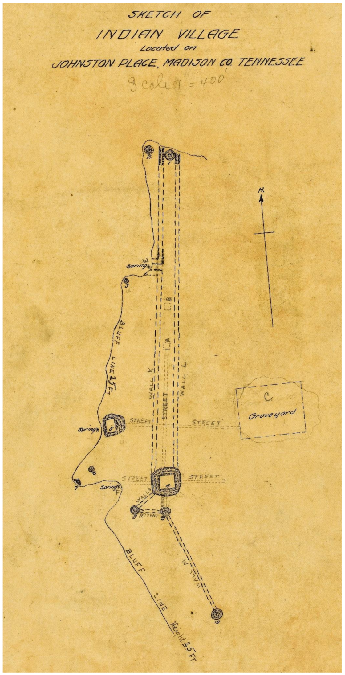
Previous Research and Cartography at the Johnston Site

Eastern North America has a long history of naturalists, antiquarians, and early professional archaeologists mapping indigenous earthen monuments [53,54,55,56,57]. Sometimes these people had professional backgrounds in surveying, sometimes they did not. It was not uncommon for some well-funded researchers to hire local surveyors to conduct mapping projects. Today, archaeologists using modern technologies like GIS software and aerial and terrestrial remote sensing methods are documenting the mixed successes of these early site surveys [2,22,58,59]. LiDAR, and geophysical surveys across eastern North America have shown that sites mapped more than 150 years ago were sometimes quite accurate. However, sometimes features were drawn differently than we might be able to discern today. These differences may relate to simple mistakes, generalizations, or overactive imaginations.
Like Pinson, the Johnston site was initially investigated by William Myer, an associate researcher of the Smithsonian Institution, who hired local civil engineer E. G. Buck to produce maps of both sites in 1917 [30] (p. 32), [49] (p. 52). However, unlike Pinson, the early map of Johnston arranged by Myer [60] has not been sufficiently reexamined using modern methods (e.g., [49,59]) to determine what this landform looked like at the time of early European expansion into West Tennessee. This is important to understand the broader Middle Woodland landscape along the SFFDR because the work of Mainfort and colleagues [59] identified numerous discrepancies in Myer’s 1922 map of Pinson. For instance, they argue the elaborate enclosure walls that span the exterior boundaries of Pinson, as well as the “Inner Citadel” and their associated intersecting mounds, might not have existed, and thus may have been embellished or severely impacted by plowing. Identifying such discrepancies led to the title of their article “Mapping Never-Never Land”, from which we derive the title of our article.
Figure 3. The Johnston Site. (a) Aerial photograph of Johnston during 2015 field season. Numbers reference mounds easily visible upon ground inspection; (b) LiDAR-derived visualization of Johnston. Map produced in ArcGIS 10.6 using a 1-m resolution digital terrain model (DTM) and the Relief Visualization Toolbox [61,62] by overlaying a Sky-view visualization at 50% opacity onto the color-stretched DTM displayed at three standard deviations and set to refresh with the display extent. Numbers reference easily visible mounds.
Remotesensing 12 02364 g003
The work of Mainfort et al. [59] provides a cautionary lesson on cartographic ‘artifacts’ and the potential for embellished earthen architecture at Johnston. Nevertheless, to begin understanding earthen monuments at Johnston, and identifying how they might have changed since their initial mapping, we had to begin by assessing the original map of the site as first published by Kwas and Mainfort [30]. We use the 1917 map as a comparative documentation of the site prior to more than 100 years of agricultural impact. The full sketch map of Johnston depicts 10 mounds situated on a north-south oriented terrace (Figure 2). The details of this map are described in an unpublished manuscript by Myer [31] and discussed in detail in an article by Kwas and Mainfort [30].
The two platform mounds (Mounds 4 and 5) at the center of the site are the largest and most visible today (see also Figure 3). A pair of conical burial mounds (Mounds 1 and 2) are drawn at the northern edge of the terrace. Only Mound 1 is currently still visible. Three additional small conical mounds are situated along the bluff line that rises above the SFFDR floodplain (Mounds 3, 6, and 7), while three more small conical mounds are drawn south of Mound 4 (Mounds 8, 9, and 10). The dimensions of these monuments as they appeared in 1917 were recorded (Table 1) and provide baseline measurements that we can compare to the results of our research presented here. Low-lying parallel embankments (Walls K and L) are discussed as once being 3 m wide and 0.75 m tall and depicted on the Johnston map to have extended from Mound 4 north to Mound 1, leaving an open turn west near Mound 3 that led to a spring at the base of the bluff. Myer discussed the embankments being most visible in 1917 at either side of Mound 1, where they are drawn as solid constructions. Elsewhere on the map of Johnston, the parallel embankments and other walls are represented by dotted lines, indicating they were ephemeral or proposed to have once existed in these locations. This includes embankments (listed as ‘walls’) on the 1917 map shown to have extended from Mound 4 to Mounds 8 and 9, and from Mound 9 to Mound 10. Associated with the mounds and embankments are small features labelled ‘streets’ that Myer discussed as leading from beneath Mound 4 outward to the cardinal directions, and from Mound 5 toward the cemetery (i.e., ‘Graveyard’ on the Johnston map). Very little is known of the cemetery and it was not surveyed during our work because it is located on private property. Within the parallel embankments between Mounds 1 and 4 are two roughly 13.5 × 13.5 m rectilinear features labelled ‘A’ and ‘B’. These are described as ‘structures’ (i.e., buildings) because daub was visible in the soil at these locales when plowing occurred. Springs are also listed along the base of the western edge of the terrace.
Kwas and Mainfort’s work on the Johnston site included site visits and examinations of surface-collected artifacts by residents who lived near the site. Their visits called into question whether any of the embankments ever existed; they commented that none of them were present during their site survey in the early 1980s. Moreover, they noted that only Mounds 1, 4, and 5 were visible and could be confirmed as indigenous earthen architecture. An examination of ceramics collected from the site suggested contemporaneity with the nearby Pinson Mounds. However, their analysis of projectile points and fragments from Johnston site differs significantly from such tools recovered from Pinson. While projectile points from Pinson can be characterized by Middle Woodland stemmed variants, the tools from Johnston are dominated by Late Archaic variants (ca. 4000–1000 BC). From the ceramic and lithic evidence at Johnston, Kwas and Mainfort suggest that the Johnston site was a potential predecessor to Pinson Mounds, with the mounds constructed around the first century B.C. [30] (p. 39).
Applying a multi-staged [11,58,63] and multi-scalar remote sensing approach to Johnston provides an opportunity to thoroughly assess the accuracy of the 1917 historic map of the site, in addition to its descriptions of mapped earthen monuments. This approach integrating LiDAR-derived imagery and multi-instrument geophysical surveys allows us to harness the strengths of both techniques, and in doing so, fully realize the topographic and subsurface signatures of pre-Contact human manipulation of this terrace landform.

3. Materials and Methods

3.1. LiDAR-Derived Imagery and Examination of the Johnston Site’s Historic Map in GIS

Aerial LiDAR integrates laser scanners, airborne vehicles (e.g., airplanes, helicopters, or drones), and highly accurate geospatial positioning instruments like real-time kinematic global positioning systems (RTK GPS) to record a diverse range of reflection information [64,65]. LiDAR-derived datasets are publicly available through most state governments in the U.S. This is because the method holds great potential for applications in a variety of civil and research sectors that span environmental hazard and ecological studies to heritage management and archaeology. However, the quality of publicly available LiDAR datasets varies. We obtained LiDAR-derived digital terrain models (DTMs) from the State of Tennessee (https://www.tn.gov/finance/sts-gis/gis/gis-projects/gis-projects-elevation), which has high-resolution coverage for most of the state. LiDAR data across our project area along the SFFDR was collected in the winter of 2011 and 2012 in collaboration between the United States Army Corps of Engineers (USACE) and the Tennessee Division of the United States Department of Agriculture’s Natural Resources Conservation Service (USDA NRCS). Data were collected with a nominal pulse spacing no more than one point every 70 cm. Downloadable bare-earth DTMs were produced from these data that were geospatially referenced using the NAD 1983 horizontal datum and the NAV 1988 vertical datum. The DTMs were tested to 1 m horizontal, and ≤18 cm vertical accuracy.
We created a LiDAR-derived hillshade visualization of the Johnston DTM in ArcGIS 10.6 by ESRI (Redlands, CA, USA) for preliminary analysis by altering the DTM symbology to display the topographic data in greyscale using the hillshade effect (Stretch Type: None; Z factor: 0.075). However, recent LiDAR-based archaeological research has highlighted numerous issues in identifying and interpreting landscape features from uni-directional hillshades alone [66,67,68]. Therefore, we also applied a suite of visualization methods available in the Relief Visualization Toolbox 2.2.1 (RVT; Institute of Anthropological and Spatial Studies, Ljubljana, Slovenia) [61,62] to the DTMs in order to better assess the presence or absence of landscape features at the Johnston Site. These included multi-directional hillshade (16 directions, sun angle 35°), principal components analysis (n = 3) of the multi-directional hillshade, simple local relief model, sky-view factor, positive and negative openness, and local dominance. Each visualization technique offers enhancement or deemphasis of topographic characteristics that allow archaeologists to elucidate the presence or absence of subtle landscape features (see Table 2). In-depth descriptions of these visualization methods can be found in [61,62,69]. When assessing the RVT imagery, we often created ‘blended’ images to enhance the RVT outputs with reference to the original LiDAR-derived DTM or other RVT imagery. An example of one blended image we used can be seen in Figure 3b, where we overlaid the Sky-view factor depicted in a greyscale color stretch at 50% opacity over the color stretched DTM. This helped us understand the correlation of subtle elevation changes to the range of values for height above mean sea level. Another blended image we used included overlaying the Sky-view factor depicted in a greyscale color stretch at 50% opacity over the Local Dominance imagery depicted in a color stretch. This blended imagery is presented and discussed in our results but offered better clarity for subtle elevation changes in both the Sky-view and Local Dominance imagery. To assess the validity of the 1917 Johnston map against the LiDAR-derived visualizations we created of the site, we georeferenced the 1917 map over an analytical hillshade visualization of the DTM in ArcGIS 10.6 using the ‘Adjust’ transform and adding control points on the 1917 map to the three most intact earthen mounds visible at the site today (i.e., Mounds 1, 4, and 5).

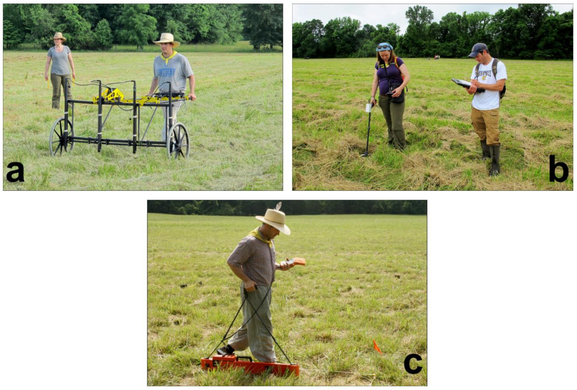
3.2. Magnetic Gradiometer Survey

Magnetometry has become one of the most frequently applied near-surface geophysical survey methods to archaeological research. As such, it has received extensive discussion on the foundation of the technology [8,71,72]. We utilized a Foerster Ferex 4.032 DLG Karto 4-sensor fluxgate gradiometer (Institut Dr. Foerster GmbH & Co. KG, Reutlingen, Germany) to survey 14.25 ha of open field space at the Johnston Site (Figure 4a). Data were collected on a 40 × 40 m grid system that was laid out using a Topcon RTK GPS (Livermore, CA, USA) and a Trimble robotic total station (Sunnyvale, CA, USA). Raw data were collected at a 0.5 × 0.1 m resolution.
Gradiometer data were processed in TerraSurveyor 3.0.36.0 (DW Consulting, Barneveld, The Netherlands) using typical destagger, destriping, and low pass filter processes prior to interpolating the data to a 0.1 × 0.1 m resolution for georeferencing in ArcGIS 10.6.

3.3. Large-Area Surface Magnetic Susceptibility

Magnetic susceptibility is a measure of a soil’s ability to be magnetized when introduced to an artificial magnetic field [73,74]. Increased magnetic susceptibility has been identified as a proxy for cultural activity (e.g., low-intensity fires, midden formation, soil movement & manipulation) [6,75,76,77]. We collected large-area surface magnetic susceptibility data to complement the results of our gradiometer survey and aid in its interpretation, as well as provide a coarse resolution ‘reconnaissance’ survey of areas we could not survey with the cart-based gradiometer used in this study (cf. [78]). We collected volume magnetic susceptibility using the Bartington MS2 m and MS2D field loop (Bartington Instruments, Oxon, UK) across approximately 24 ha of the Johnston Site (Figure 4b). Data were collected in 20 m increments and spatially situated with a handheld GPS. Recorded data were an average of three readings spaced 10–20 cm apart. The instrument was zeroed prior to each reading. In some areas where we identified ‘hot spots’ of high magnetic susceptibility (mounds and non-mound open areas), we increased the resolution of our horizontal coverage from 20 m to 5 or 2 m. Data were visualized in ArcGIS as color-coded points, in addition to a raster interpolated using nearest neighbor gridding.

3.4. Electromagnetic Induction

Electromagnetic induction meters (EMI) measure subsurface phenomena by emitting an electromagnetic field and measuring the response to that field as it is moved around the survey area [73,79,80,81,82]. Slingram EMI instruments can measure two responses to the electromagnetic field, the Quadrature-phase (QP), which represents apparent soil conductivity, and the In-phase (IP), which represents apparent volume magnetic susceptibility. Some EMI instruments can do this simultaneously. For instance, the Geonics EM38-MK2 (Geonics Limited, Mississauga, ON, Canada) we used in this study measures QP and IP at two different depths simultaneously (Figure 4c). This instrument has electromagnetic coil separations of 0.5 and 1 m, resulting in an approximate maximum depth penetration of 0.75 m and 1.5 m for conductivity data, measured in millisiemens per meter (mS/m), and 0.3 m and 0.6 m for magnetic susceptibility data, measured in parts per thousand (ppt) when operated, as we did, in the vertical dipole mode. Data were collected every 0.5 m along transects spaced 0.5 m apart. Data were downloaded and processed using the TerraSurveyor software package, with typical application of despike and either high-pass or low-pass filter operations applied before being interpolated to 0.25 m pixels and exported to ArcGIS.

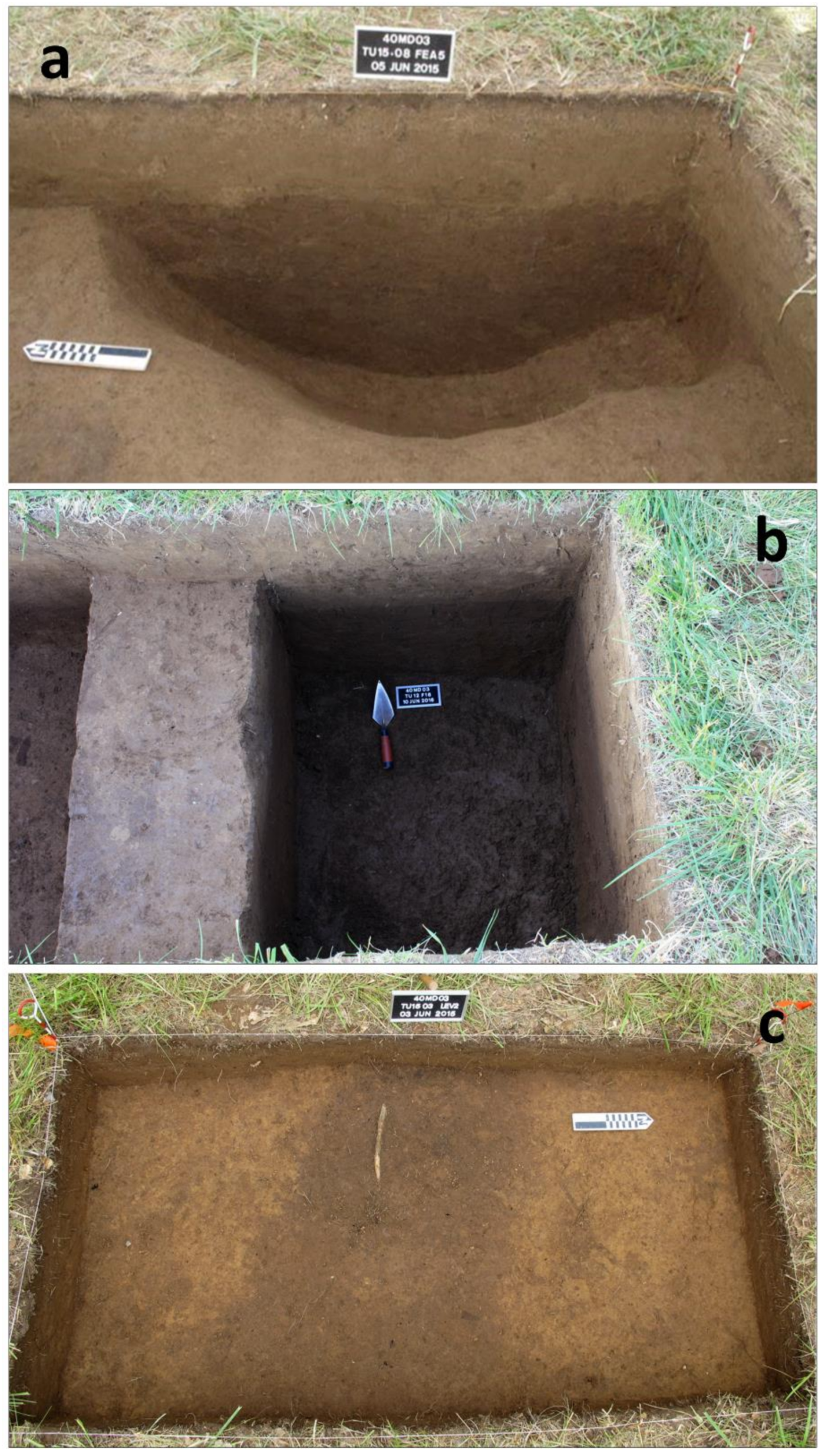
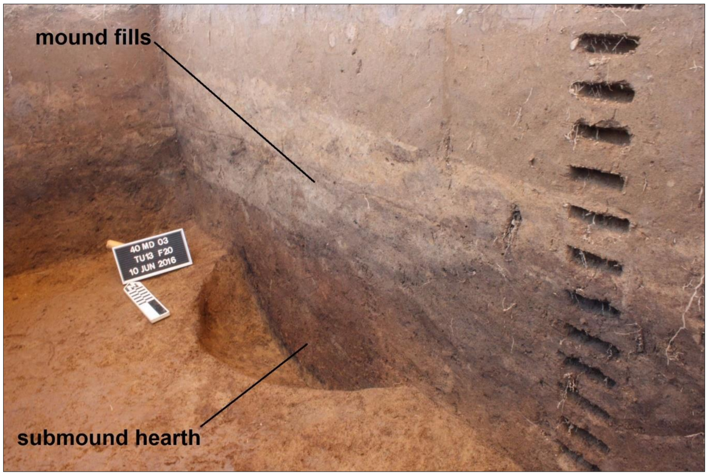
3.5. Test Excavations of Geophysical Anomalies

After our LiDAR-derived imagery and geophysical datasets were processed and analyzed, we examined a non-random sample of the identified topographical and geophysical anomalies through test excavations. Excavations were conducted in a range of trench sizes, by hand, in arbitrary 10 cm levels until intact features were identified. We screened a 10–25 percent random sample of all excavated non-feature soil matrix (e.g., plowzone) using 6.35 mm (0.25″) mesh. The entirety of all features we identified and excavated were processed using water flotation. This excavation methodology ensured a sufficient sample of displaced non-feature artifacts, and the total recovery of artifacts and ecofacts from feature contexts. The test excavations are presented in detail elsewhere [83]. The excavations we discuss here are intended to provide the reader examples of how our integrated remote sensing approach led to success in identifying surface and subsurface archaeological features that help us enhance our understanding of this important site, and better situate it within the Pinson ritual landscape [83].

4. Results

In this section, we present the results of our analyses of LiDAR-derived imagery and geophysical surveys at the Johnston Site. We begin with a comparison of the LiDAR-derived imagery and the 1917 map of the Johnston Site. We then move to discuss the results of the large-scale magnetic gradiometer and magnetic susceptibility surveys before discussing the EMI results. Test excavations of topographic and geophysical anomalies are presented when applicable.

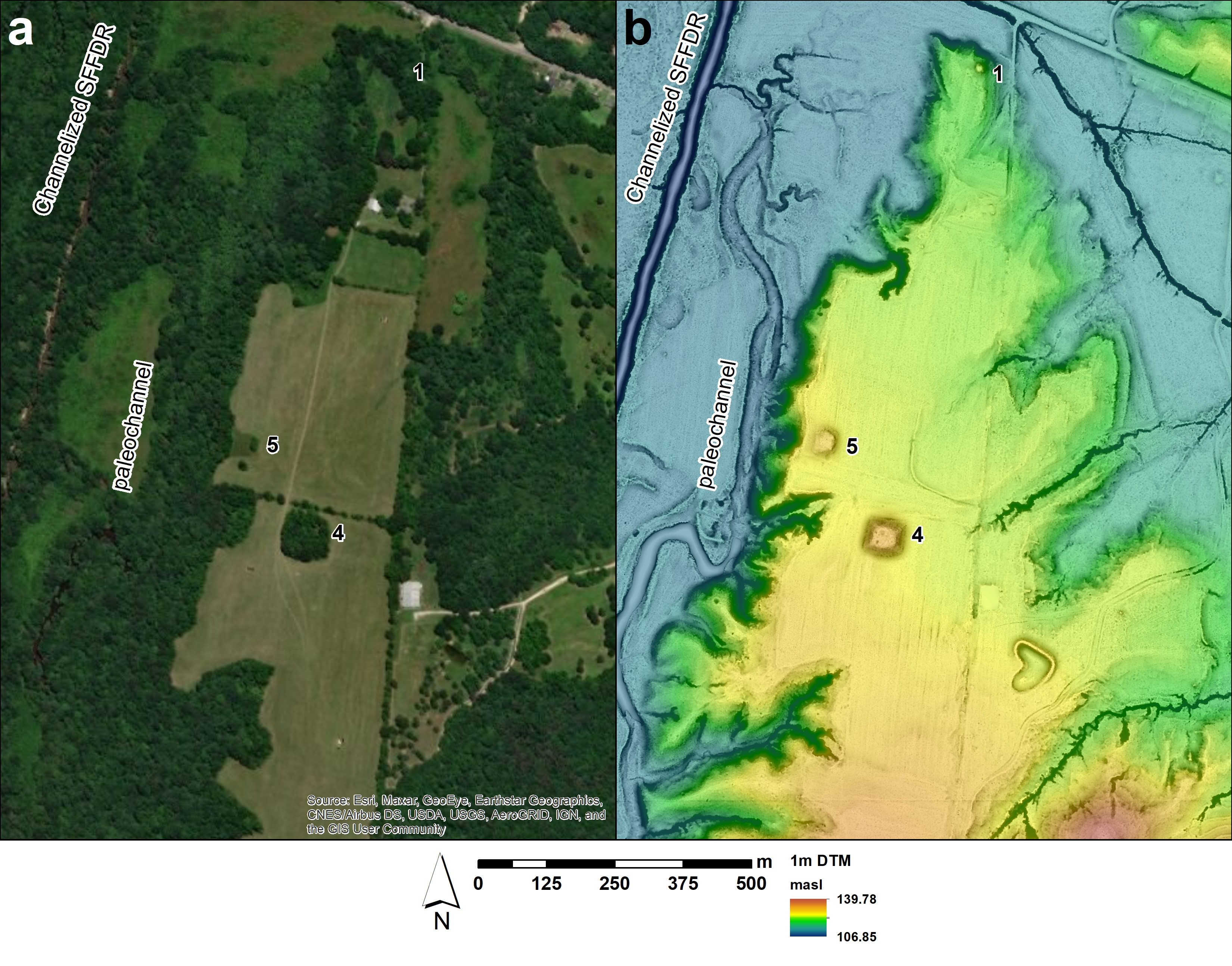
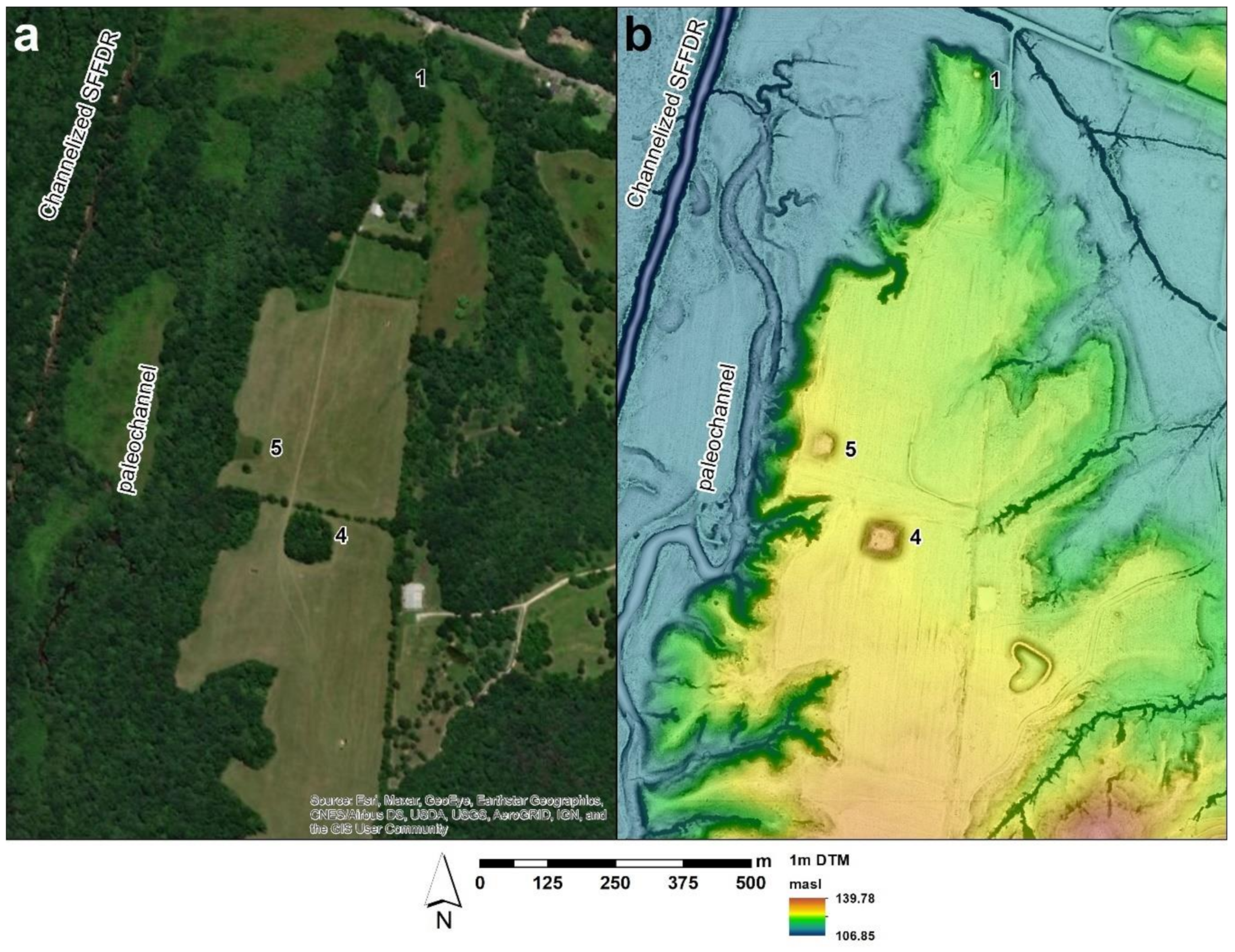
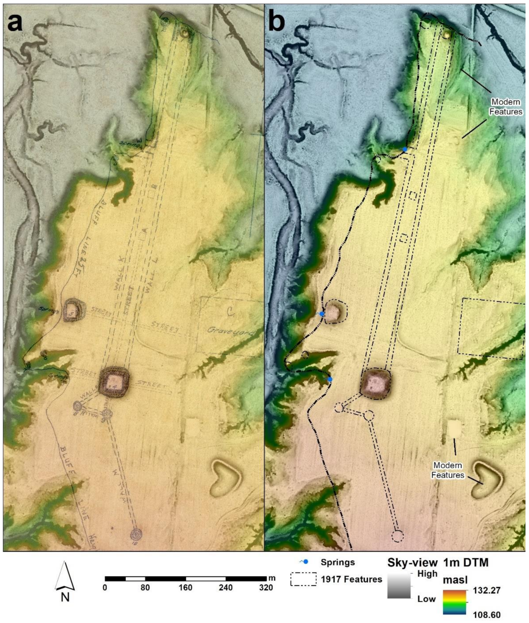
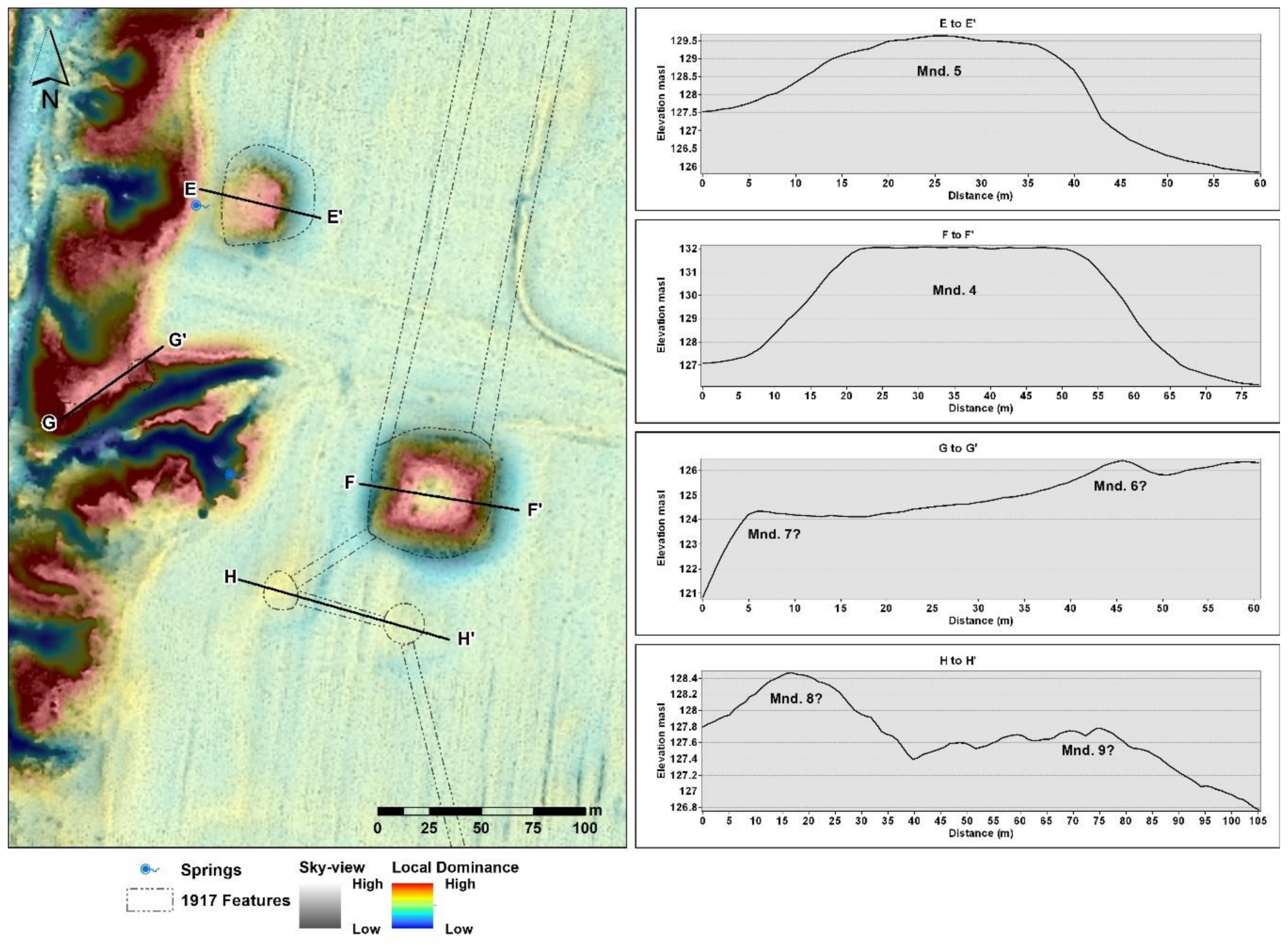
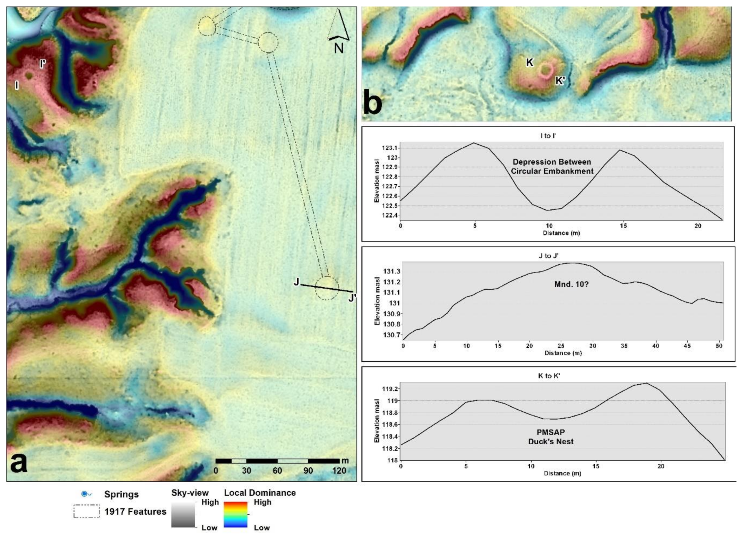
4.1. Analysis of LiDAR-Derived Imagery Compared with the 1917 Map of the Johnston Site

Overlaying the 1917 map based on E. G. Buck’s survey work at Johnston over our LiDAR imagery allowed us to compare Buck’s cartography and Myer’s descriptions with the current state of topographic relief at the site (Figure 5a). It also allowed us to examine the Johnston landscape for topographic features not included on the 1917 map. Using the three clearly visible mounds at the site as anchor points for georeferencing the 1917 map to real world coordinates, we were able to confidently determine correlations and differences in topographic features between the maps. After redrawing Buck’s features as polygons, we could determine where a given mound or embankment should be in relation to topographic features identifiable in LiDAR-derived imagery (Figure 5b).
The first discrepancy we can easily identify is the 1917 bluff line that undulates along the western edge of the terrace landform. In some areas the bluff edge is depicted 60 m or more east of where the bluff is. In others, the 1917 bluff line is depicted west of the current bluff line, now dominated by incised erosional gullies. While the former can be attributed to ‘sketching in’ the bluff line as a feature relative to other earthen monuments, there may have been areas where the 1917 bluff line was more accurately depicted. If this were the case, we could assume that the erosional gullies present in areas that were depicted as level terrace in 1917 provide a proxy for landform evolution since the map was drawn. These two scenarios are hard to assess given the identified discrepancies between the Buck/Myer map and current topography at Pinson [59].
According to the 1917 map, the northern extent of Johnston supposedly contained Mounds 1–3 and some of the best-preserved portions of the parallel embankments. Our LiDAR-derived imagery shows that Mound 1 is still present at Johnston, conical in shape, but smaller in height and base diameter than described in 1917 (Figure 6; A to A’). Mound 2 is hard to evaluate. A topographic rise that is roughly 0.2 m in height is present in the approximate location of Mound 2 but there is no clear shape to this feature. This may be because much of Mound 2 area has eroded into the gully to the north. However, it is equally possible that this is a relic of natural topography and was interpreted as a built earthen feature in 1917. Determining whether this topographic feature is natural or cultural will require future investigations and maybe excavation.
Descriptions of the parallel embankments indicate the best-preserved sections extended south of Mounds 1 and 2. Our analyses of LiDAR-derived imagery and topographic profiles shows that two parallel rises exist directly south of Mounds 1 and 2 (Figure 6; B to B’). These features are both close to 15.5 m wide and 0.3 m in height. They extend approximately 80 m to the south before no longer being clearly visible in elevation profiles or other visualization methods. However, an elevation profile across the purported location of these features in a former agricultural field 300 m south of Mound 1 (Figure 6; D to D’) does suggest very subtle parallel rises are present but only 0.04 or 0.06 m tall.
The location of Mound 3 is slightly off from our georeferencing of the 1917 map. However, it is still visible as a conical mound, albeit smaller in height and diameter than the reported dimensions in 1917. Our results estimate that it is roughly 7 m in diameter and 0.3 m tall (Figure 6; C to C’). Mound 3 is currently in a precarious position, situated on a relict finger-like landform directly between two deep erosional gullies.
The central portion of Johnston has the two largest mounds (4 and 5) recorded at the site, in addition to four small conical mounds situated near them (Figure 7). Mounds 4 and 5 are still easily visible on the ground and in our data visualizations. Mound 5 was listed as a polygon in the 1917 map but appears more like a deflated low-lying rectangular mound in our topographic visualizations. The impact of agricultural plowing may have caused, or at least contributed, to this slight change in shape. Currently, Mound 5 is roughly 3.6 m tall and is 39.3 × 45.3 m in size at its base, while the surface spans 22.9 × 25 m (Figure 7; E to E’). Mound 4, the largest mound at Johnston, is a classic rectangular platform mound measuring 5.8 m tall, 57 × 59.5 m at the base, and exhibiting a surface extent of 32.8 × 34.6 m (Figure 7; F to F’). Multiple circular depressions on the surface of Mound 4 are visible, suggesting either looter attempts to recover artifacts from the mound, or potentially concavities from tree falls.
On a narrow finger-like residual landform that extends west toward the SFFDR floodplain between Mounds 4 and 5 is the location of two small conical mounds. These are labeled Mounds 6 and 7 in the 1917 map. Mound 6 is the more visible of the two, potentially because it is situated at the center of this landform. Mound 6 is about 5.9 m in diameter at the base, and roughly 0.4 to 0.5 m in height. Mound 7 is harder to evaluate. It is positioned at the edge of the landform, surrounded by erosional gullies. The 1917 map describes it as a ‘half oval’ or crescent. We can distinguish a roughly 0.3 m rise at the edge of this landform but if this is the remnants of an earthen mound, very little remains intact. The small rise extends 4 m from the edge of the landform and measures roughly 7 m north to south (Figure 7; G to G’).
Mounds 8 and 9 on the 1917 map are situated south of Mound 4 and connected via purported earthen ‘walls’. We can detect no topographic evidence of earthen walls that connect these three mounds to one another. Moreover, it is not clear that the subtle topographic relief associated with the location of these two mounds confirm human construction. If they are built earthen architecture, then of the two, Mound 8 is the most visible in our imagery analyses. It measures 20 m in diameter and is roughly 0.6 m in height. Mound 9 is much harder to discern in LiDAR-derived visualizations and topographic profiles. Still, a topographic rise is present in the area where the 1917 map denotes the location of this feature. This rise is 20 m in diameter and 0.2 m in height (Figure 7; H to H’).
According to the 1917 map of Johnston, the southern portion of the site contains an earthen wall that extends to a conical mound, Mound 10. Like the walls connecting Mounds 4, 8, and 9, no surficial evidence of this earthen wall exists. However, there is a clear topographic rise associated with the purported location of Mound 10 (Figure 8a; J to J’). In this case, our LiDAR-derived visualizations suggest that this rise associated with this area is 0.4 m tall and roughly 25 m in diameter. Like Mounds 8 and 9, it is not clear from topographic analyses alone that this is a human-made feature. We discuss below how we confirmed it as such. An exciting and unexpected discovery in our examination of LiDAR-derived imagery of the southern portions of the Johnston Site comes in the form of a non-mound feature that was not in the historic survey of the site. West of Mound 8 and 9 we discovered a depression encircled with an embankment. This feature is morphologically like the feature designated the “Duck’s Nest” at PMSAP (Figure 8a; I to I’; Figure 8b; K to K’) [49] (pp. 155–158).

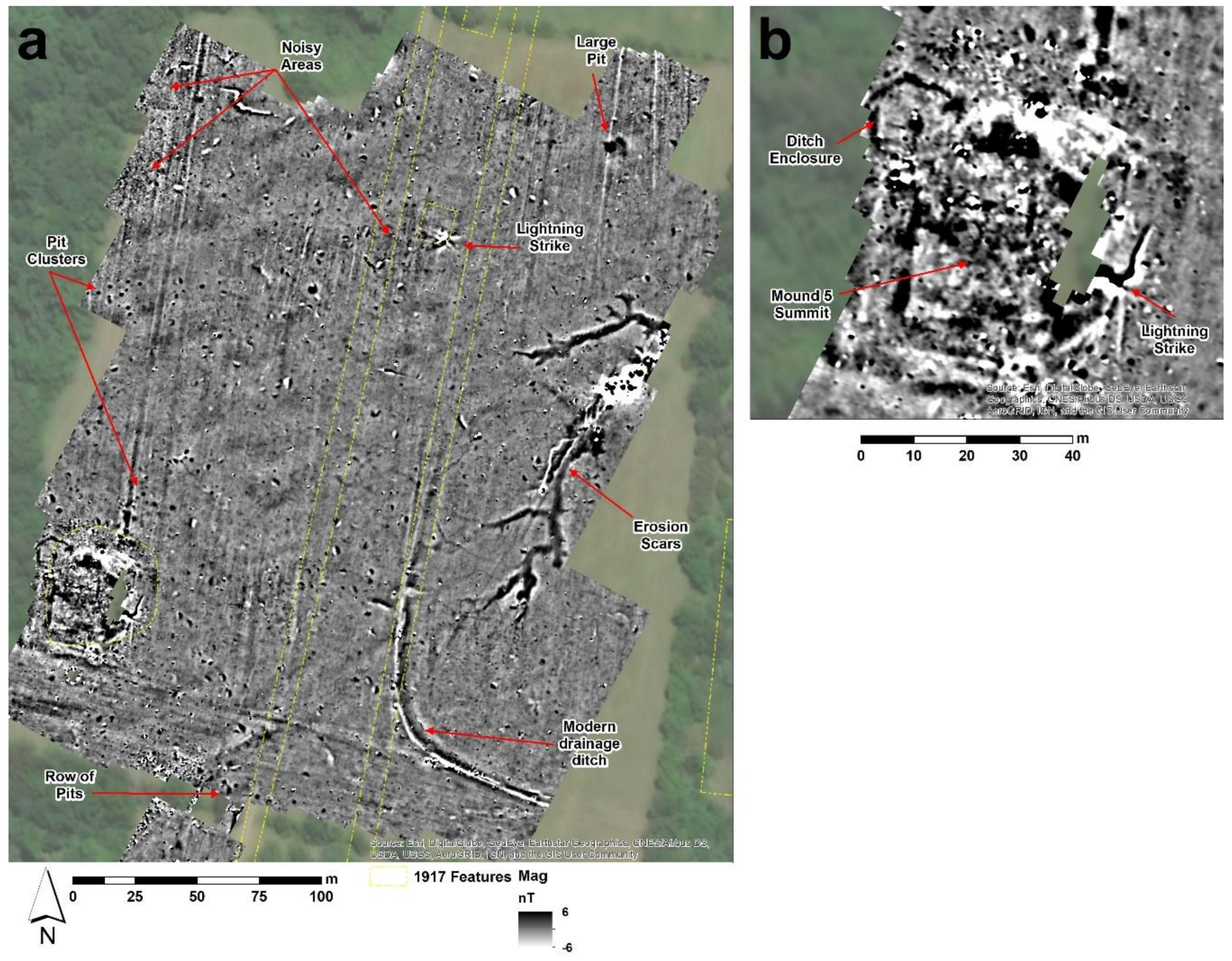
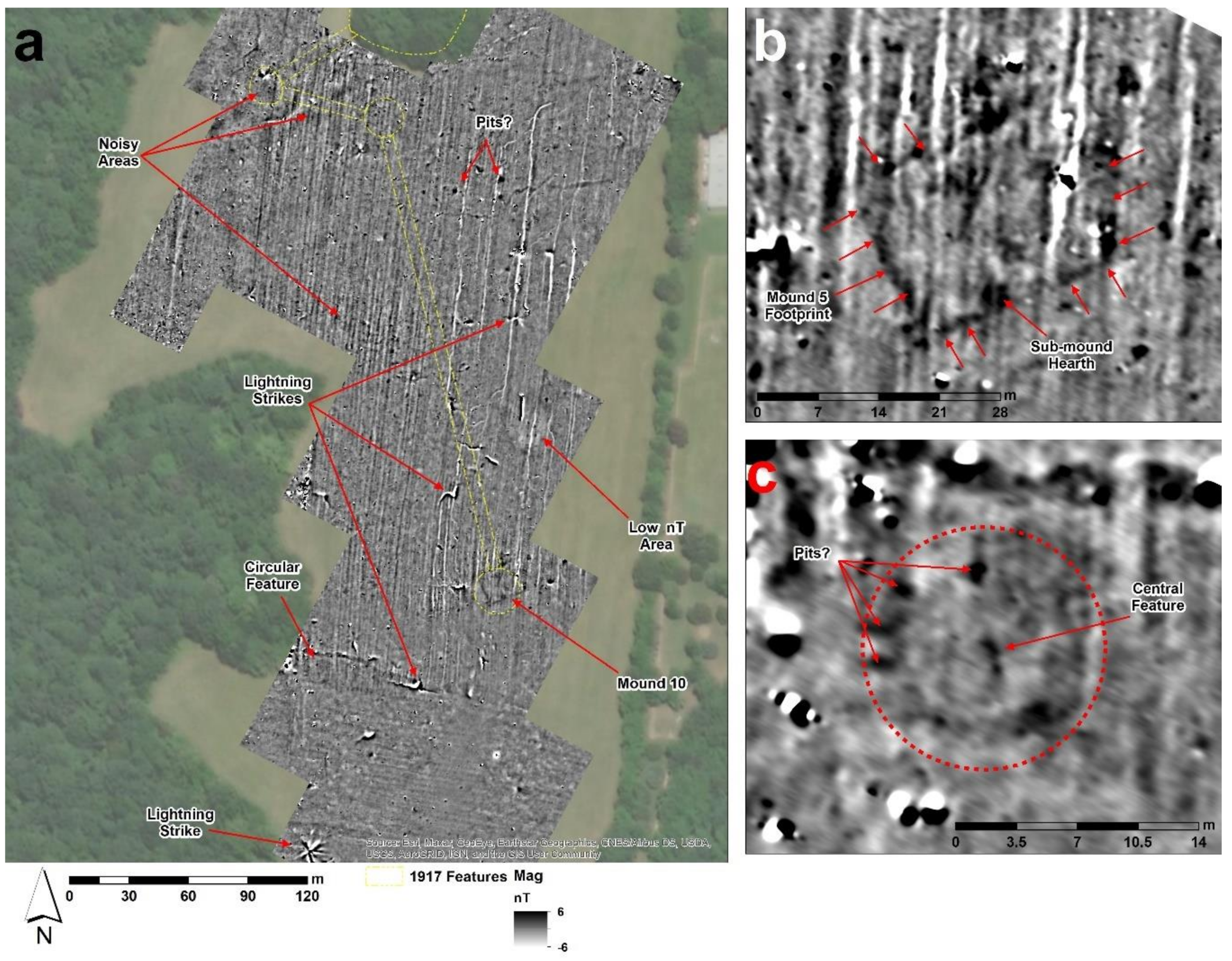
4.2. Gradiometer Results from the Johnston Site

Our gradiometer survey of Johnston was limited to the central and southern portions of the Johnston Site, where large open spaces could easily accommodate our cart-based instrument. There are also areas with large amounts of metal in the northern portions of the survey area that would make a gradiometer survey unsuccessful. Viewing the full extent of our magnetic coverage brings into focus the magnitude of agricultural plowing and drainage modifications in this portion of the site in the historic era (Figure 9). Intensive plow scars are seen in the data trending north-south, with the exception of the extreme southern portion of the survey area, where scars trend east-west—an indication of a former field boundary. Some plow scars are intense, potentially reflecting early deep-chisel plowing. The long history of agricultural practices seen in the gradiometer data undoubtedly impacted the topography of small features like the purported 1917 parallel embankments and smaller mounds. We can also identify the remnants of several lightning strikes across our survey area, something more archaeologists are discussing in recent research (see [84]).
We focus our discussion on results from selected magnetic features examined in test excavations that offer insight for our research questions outlined here. To begin, in the northern half of our gradiometer survey we were able to delineate numerous clusters of pit features denoted by rounded and spatially distinct magnetic highs (Figure 10a). Limited test excavations of a sample of these features have shown that they are either hickory nut (Carya sp.) roasting pits or storage pits with little to no cultural material but are filled with dark organically enriched material. Several pits are aligned in a row to the north of Mound 4, suggesting not only the spatial contemporaneity, but potentially association with Mound 4 as well. Test excavations of one pit in this group revealed a dark fill but no diagnostic cultural artifacts to associate the feature with a specific time of use (Figure 11a). We have several charred botanical samples that have been submitted for AMS 14C dating, but those dates are the focus of another article we are preparing.
A large irregular feature measuring nearly 11 m in diameter is visible in the northeastern portion of our gradiometer data. Test excavations revealed a deep (>1 m) pit refilled with comparatively dark organic sediment (Figure 11b). Unfortunately, this feature contained no diagnostic artifacts to denote when the feature was used or refilled. In between the area where parallel embankments were mapped in 1917, and where the potential ‘structure A’ was situated (evidenced by burned daub present in plowed soil), we discerned the magnetic remnants of an isolated lightning strike roughly 12 m in diameter. Soils below plow zone were examined through a test excavation in this area and were documented as a reddish clayey sand. Plow scars cutting into this reddish horizon were visible below the plow zone. Therefore, it is possible that the structural feature ‘A’ mapped in this locale in 1917 was the result of a lightning strike. However, further research must be conducted to confirm this hypothesis. It is interesting to note that a noisy area of magnetic gradient borders the lightning strike to the west and southwest. This dense area of subsurface magnetic features likely represents a concentrated area of past human activity. Additional areas of seemingly ‘noisy’ magnetic phenomena are represented by non-patterned high and low magnetic features visible to the northwest of the locale inside the parallel embankments mapped in 1917. These can be characterized by high magnetic susceptibility due to the intensity of the response to plowing in this area. No magnetic response correlates with the location of the parallel embankments, leaving us wondering whether subsurface remnants of these features still exist.
Gradiometer results associated with Mound 5 are particularly intriguing. Our results identify a rectangular platform shape to this mound that contradicts the 1917 descriptions of the mound as a polygon. This discrepancy is likely the result of the intensive plowing at the site. The summit of Mound 5 exhibits numerous magnetic features potentially associated with platform activities. A lightning strike is visible on the eastern flank of the mound. However, most interesting to this area is a small ditched enclosure that we identified under the northern flank of Mound 5. This feature is morphologically like those identified in the Middle Ohio Valley and associated with Hopewellian ritual activity. The ditch encloses approximately 185 m2 and exhibits a magnetically enhanced feature 3 m in diameter at its center. A test unit cross-cutting a small section of the ditch confirmed this interpretation and revealed the ditch contained burned earth and dense amounts of charcoal, suggesting the termination of the enclosure was intentional and likely occurred prior to the construction of Mound 5 (Figure 11c).
Gradiometer results from the fields south of Mound 4 raise additional questions about the indigenous landscape. Gradiometer coverage over Mounds 8 and 9 are noisy and reflect isolated higher magnetic susceptibility in these areas, visible in the non-uniform magnetic characteristics of the plow scars between the mounds (Figure 12a). However, no clear association is visible between the mound locations and our data, leaving questions to whether the mounds mapped in 1917 are now less visible due to plowing, or if they are relicts of natural topography. There are no clear clusters of pits south of Mound 4 like we see north of the mound. However, some individual pits can be discerned southeast of Mound 4. An area of low magnetic gradient is present in the southern field with four potential pits situated at the center of the area (Figure 12a; Low nT Area). We mapped numerous lightning strikes across this open area south of Mound 4.
The area mapped historically as Mound 10, which has no topographic relief, was among the significant outcomes of our assessment of the magnetic data. Here we identified a rectangular feature and a round pit, both tested in a 1 × 10 m long trench (Figure 12a,b). These results suggest there was a mound present, but it was likely rectangular and not round or conical. The magnetic response to Mound 10’s base dimensions may reflect magnetically enhanced topsoil that eroded over time to the bottom of the mound, revealing a 27 × 20.5 m base dimension.
Test excavations confirmed the presence of at least two different mound fills related to Mound 10’s construction and identified a small basin shaped hearth under the mound fill. Analyses continue to assess how these features relate to one another. (Figure 13). A small clay cooking ball was recovered from the mound fill. Artifacts like these imply a Late Archaic (ca. 4000–1000 BC) presence on the site [85]. Additional excavations and a robust radiocarbon dating program is needed to confirm the construction age of Mound 10.
Southwest of Mound 10 we identified a potential circular post structure 10 m in diameter (Figure 12c). This feature appears similar to other post-enclosures or paired-post structures in the Middle Ohio Valley [2,22,36,86,87,88,89,90,91]. We have yet to test this feature with excavations; however, the exterior of the circular feature appears to have numerous possible pits associated with it. A central magnetic feature is also present within this circular structure. This may be a central hearth, a depositional or refuse feature, or a central post. Excavations should clarify the nature of this structure.
To summarize, the results of our gradiometer survey at Johnston revealed numerous subsurface magnetic features that exhibit no topographic relief. The identification of such features allows us to discern activity areas across space in ways LiDAR-derived imagery do not. The gradiometer data have little correlation with some of the built features outlined on the 1917 map, such as the parallel embankments north of Mound 4 and the ‘streets’ or ‘walls’ that connect Mounds 8 and 9 to Mound 4. Moreover, there is little evidence that Mounds 8 and 9 exhibit clear magnetic signatures, leading us to question the nature of their existence. The gradiometer data over Mound 5 reveals the original shape of the mound to be rectilinear and shows that a uniquely different monument, a small ditched enclosure, preceded its construction.

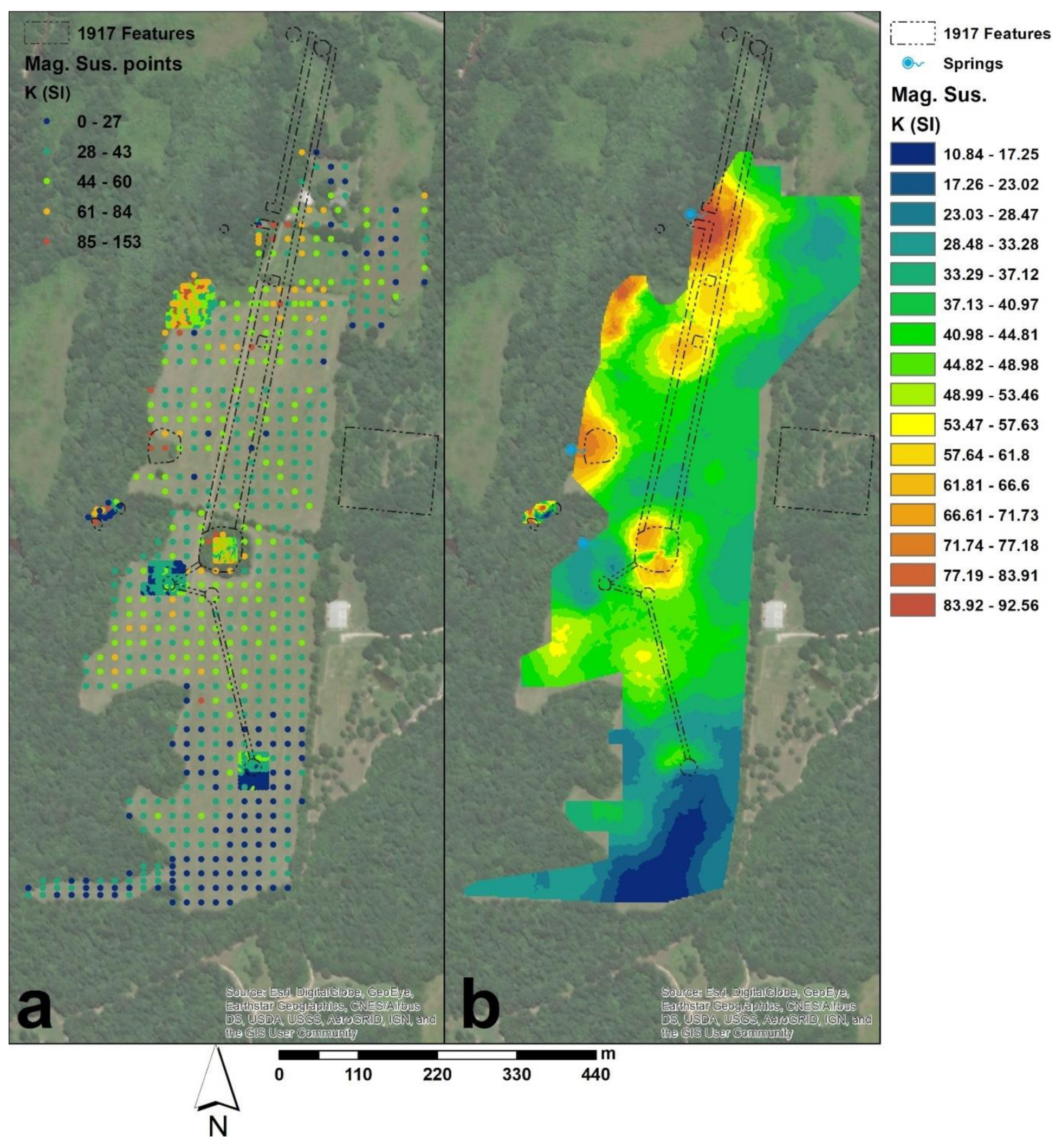
4.3. Results from Large-Scale Surface Magnetic Susceptibility Surveys at the Johnston Site

Our large-scale surface magnetic susceptibility survey at Johnston was intended to complement the results of our gradiometer and LiDAR imagery survey and analyses. By examining the magnetic nature of the near-surface across the site, we hoped to better understand the accuracy of the 1917 map, interrogate the noisier portions of the gradiometer survey, and examine areas of the Johnston Site that we were not able to survey with our cart-based gradiometer or that contained large amounts of metal.
The results of our magnetic susceptibility survey exposed multiple areas of high susceptibility likely related to past human activities. We consider these ‘activity areas’ in the broadest sense of the term. North of Mound 4, the highest readings and largest activity area spatially coincides with the western opening in the parallel embankments from the 1917 map (Figure 14b). Probably not coincidentally, this entrance area leads to one of the springs denoted on the 1917 map. This suggests either a long history of pre-Contact indigenous people accessing this natural feature, or a short and intensive period of activity around the spring. Other large activity areas north of Mound 4 identified by spatially-distinct areas of high magnetic susceptibility correlated with the ‘A’ and ‘B’ purported structures inside the parallel embankments on the 1917 map, as well as an area situated along the tree line to the west of these structures. While we do not have gradiometer data over the activity area associated with the northern-most structure ‘B’ on the 1917 map, we do have comparative gradiometer data to assess correlations between the two magnetic datasets and the activity area associated with structure ‘A’ on the 1917 map and the area to the west at the tree line. The activity area associated with structure ‘A’ exhibits a large lightning strike right over the mapped structure, in addition to an area of elevated background gradiometer readings and isolated magnetic highs likely related to archaeological features (e.g., posts and pits) (see Figure 10a). The activity area at the tree line exhibited what we characterize as high levels of ‘noise’ in the gradiometer data, stemming from intense plow scars and numerous isolated high and low magnetic features (see Figure 10a). Therefore, we consider both areas as important locales exhibiting strong evidence for past human use of the Johnston Site. Moreover, the correlation with highly magnetic plow scars in this area indicates that highly magnetic plow scars elsewhere at the Johnston Site, as well as at other sites in the eastern U.S., may be an indicator for areas that have enhanced magnetic susceptibility from pre-Contact human occupation [29].
Magnetic susceptibility data over Mounds 4 and 5 exhibit high readings associated with the mounds themselves and with areas directly adjacent to them. For Mound 5, high levels of magnetic susceptibility extend to the west of the current mound boundaries. This may be the result of historic plowing that has displaced mound fills westward, or these data may be indicating off-mound activity areas. Magnetic susceptibility data around Mound 4 show high values extending to the northwest and southeast of the mound. These values may represent erosion of mound fill in these directions. We do not have the gradiometer coverage over the northwestern areas of Mound 4 for comparison, but data to the southeast exhibits highly magnetic plow scars similar to the activity area at the tree line in the northwest portion of our magnetic survey. However, in this locale there are not as many isolated magnetic features in our gradiometer data, lending support to the hypothesis that high magnetic susceptibility around Mound 4 may be related to eroded mound fills, and the spreading of those sediments during historic plowing.
A series of magnetic susceptibility readings in tree cover over Mounds 6 and 7 show good correlations with the topographic remnants of these features and high magnetic susceptibility values. However, we also identified an oval area of high magnetic susceptibility in between the mounds that suggest a subsurface activity area or cluster of archaeological features.
South of Mound 4 our magnetic susceptibility survey shows a large area of moderately high readings. This includes the area over Mounds 8 and 9; however, a more isolated area of moderately high magnetic susceptibility is associated with Mound 8. Two isolated areas of high magnetic susceptibility lie south of where Mounds 8 and 9 were mapped in 1917. Like our survey results north of Mound 4, these two areas correlate with plow scars in the gradiometer data that appear more magnetic than those elsewhere. Therefore, we consider this as good evidence for activity areas.
Magnetic susceptibility data associated with Mound 10 was moderately high only north of the mound remnants identified through the gradiometer data, despite an increased sampling density in this area. Highly magnetic plow scars are present in this area as well, suggestive of an off-mound activity area associated with Mound 10. Low to moderately low magnetic susceptibility readings are correlated with the circular feature west of Mound 10 in the gradiometer data. This may indicate that this feature was not used for a long period of time or peripheral to more intensive activity areas in the core of the site.
The results of our large-scale surface magnetic susceptibility survey identify areas at Johnston that were likely used by humans but were absent in other remote sensing imagery (surface or geophysical). As such, it provides an important supplement to understand the spatial relationships between human activities and monumental architecture at the site.

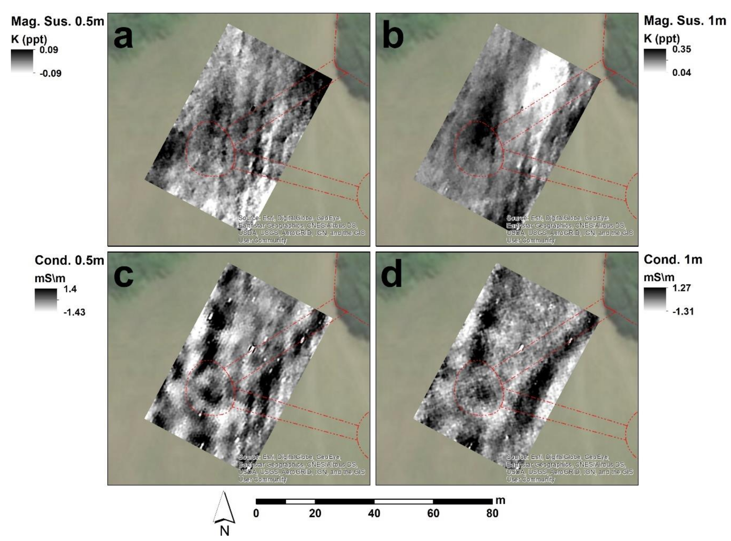
4.4. Results from an Electromagnetic Induction Survey of Mound 8

After assessing the LiDAR-derived imagery, gradiometer data, and surface magnetic susceptibility data for the Johnston Site, we were still unsure of whether a few of the small conical mounds at the site were indeed pre-Contact indigenous mounds rather than relict topography. However, we only had the opportunity to survey one with a slingram EMI meter, so we decided to focus on Mound 8.
Mound 8 has four datasets. The magnetic susceptibility data from the 0.5 and 1 m coil separations (ca. 0.3 and 0.6 m depth) show parallels with the gradiometer and surface magnetic susceptibility data. In data from both depths, this includes higher background magnetic susceptibility around the locale where Mound 8 was mapped in 1917 and the identification of isolated magnetic features that likely represent intact subsurface archaeological features associated with the topographic rise we can identify in the LiDAR-derived visualizations (Figure 15a,b). The data from the 0.5 m coil shows a transitional arc of high and low magnetic susceptibility in the southeastern portion of our survey block that mirrors the bend of Mound 8 as it was mapped in 1917.
The conductivity results of our EMI survey over Mound 8 depict no clear high values correlating with the complete coverage of the supposed Mound 8 location (Figure 15c,d). A high conductivity pattern is common among plowed down earthen mounds in the eastern U.S. because the remnants of clay-rich sediments used to build mounds often retain more moisture than surrounding soils (see [78,79,87]). However, in both the 0.5 and 1 m coil datasets (ca. 0.75 and 1.5 m depth), a high conductivity feature is present and spatially centralized over the topographic rise denoted as Mound 8. This may suggest that intact mound remnants are located here and are retaining more moisture, or there is a centralized non-mound feature under this ‘rise’. In either case, the sum of data in this locale supports an interpretation that Mound 8 is anthropogenic, although this needs to be confirmed through excavation.

5. Discussion

Our integrated application of LiDAR-derived imagery and multiple geophysical survey techniques at the Johnston Site is formulated to help untangle the complex palimpsest of pre-Contact American Indian use and construction of the landscape. Simultaneously, we implemented these techniques to interrogate the validity and preservation of built features as mapped in 1917, and in doing so, also tried to better understand the impact of modern American agricultural practices on this important site. Our results pushed us toward a more detailed understanding of the Johnston Site that no single method we employed could have offered on its own. This multi-staged approach allows us to revise the reported dimensions and forms of mounds at the Johnston Site and work toward new research questions for future work. From this perspective, in the face of increasing erosion around the edges of the Johnston site, we can use our results to provide new information toward effective site conservation.

5.1. Toward a New Map of the Johnston Site

One of the primary goals of our research was to better situate the Johnston Site within understandings of the broader Middle Woodland landscape along the SFFDR. This required a formal interrogation of the 1917 map based on the work of Buck and Myer. Because of heavy vegetation, our use of LiDAR-derived imagery offered the only way to reassess the built environment at the northern-most portion of the site. In this area, we have strong topographic evidence that Mound 1 is both authentic and similar in size to the dimensions reported in 1917 (see Table 1 and Table 3). We identified Mound 1 as nearly 2 m smaller in the base diameter but nearly the same height. One explanation for these differences in size could be attributable to the erosion of the mound surface, but this should lead to a larger base diameter. Therefore, our measurements may just be more accurate than those made in 1917, or the surveyor Buck may have directed less attention to mapping Mound 1 because it was not as large as other mounds at the site (e.g., Mounds 4 and 5).
Differences we can identify with Mound 2 are more complex to describe. A small rise is present in the location where this mound was mapped in 1917; however, the rise and the base dimensions of this rise are much smaller than what was reported previously. The placement on the edge of the Johnston terrace may indicate that much of this mound was lost as the terrace retreated. Such active erosion is visible today [83]. Alternatively, this topographic feature may be a natural relict of the landscape and its proximity with Mound 1 may have led Buck and Myer to interpret it as a. Further research is needed to confirm the nature of this rise.
The parallel embankment walls that are described from Mounds 1 and 2 south to Mound 4 are also hard to explain. In the northern reaches of the site there is strong topographic evidence for the eastern wall, and good evidence for the western wall. However, as the walls extend south into areas where we have gradiometer and magnetic susceptibility coverage, the topographic evidence is minimal and there is no correlation to geophysical signatures where the walls should be. This leaves us to question whether the history of modern agricultural plowing at the site has destroyed topographic evidence for the embankments in most unforested portions of the site. If the embankments are present near Mounds 1 and 2, but are not clearly visible further south, the early map may have continued the walls for consistency. The area northeast of Mound 3 and associated with the natural spring and western opening of the embankments shows extremely high magnetic susceptibility values for the entire site. This lends some validity to there being an important activity area in this portion of the site, but offers little support for walls or an opening to any walls here.
The location of Mound 3 as described in 1917 exhibits a clear conical rise with a nearly identical height, but like Mound 1 the base dimensions are off by nearly 3 m. This implies an error in the 1917 base measurements for this mound since any erosion should have led to a potentially larger, rather than smaller, mound base area. The two structures on the 1917 map labeled ‘A’ and ‘B’ corelate with high magnetic susceptibility. In the case of ‘A’, a lightning strike is visible in the gradiometer data. This suggests that the surveyors may have seen reddish soil discoloration in these areas and mapped those patterns as archaeological features. This said, we cannot definitively assign such an interpretation to ‘B’ because we only know that it is associated with high magnetic susceptibility. Extending our gradiometer coverage north will offer more insights into whether the ‘B’ structure is also related to a lightning strike.
There is no topographic or geophysical evidence for any of the streets or walls that connect Mounds 4 and 5, or those associated with mounds further south. However, our work does offer new insights into Mound 5, specifically its history and shape. Our topographic imagery shows that the base of Mound 5 is 2–3 m smaller than previously recorded. In contrast, the surface area is larger by about 3–4 m. This likely relates to the impact of plowing around and over this small platform. Our gradiometer data offers clear evidence for a ditch enclosure present before the construction of Mound 5. Our test excavations confirmed this feature and show preliminary evidence that it was refilled with anthropogenic materials. If the deconstruction of the enclosure and the construction of Mound 5, a platform mound, marks an important shift in the use of this space, then we can begin to build new research questions for the Mound 5 locale. For instance, Middle Woodland enclosures have been interpreted as collective monuments that imply an internal exclusivity for those who enter and use their interior spaces. These monuments are built to enclose an area, interpreted as creating a perception of ‘us and inside’ versus ‘them and outside’, and have been considered a place where people from diverse geographic scales participated in specialized ritual events [35,92,93,94,95,96]. Alternatively, Middle Woodland and Late Woodland platform mounds, while also considered monuments emphasizing collective notions of society, are commonly interpreted as socially inclusive because of their association with the remains of feasting [41,97,98,99]. We reference Late Woodland (ca. AD 600–1000) platform mounds here also because we have no relative or absolute chronological information for Mound 5; we only know that it post-dates a Middle Woodland enclosure.
The current topographic data for Mound 4 shows that the base dimensions are less by 3 and 4 m, while the surface dimensions are greater by 3 to almost 5 m. This may be a combined result of erosion and deflation of the mound surface, leading to a larger surface platform, while plowing around the mound would move mound sediments around the field, causing the base to decrease in size rather than increase from the accumulation of eroded surface sediments. Magnetic susceptibility from the surface of Mound 4 shows a combination of high and low values. These differences may relate to variation in mound fill used to construct Mound 4 or it may represent features associated with the use of the mound summit.
Our examination of Mounds 6 and 7 suggest that remnants of these features are present and can be represented geophysically by high magnetic susceptibility. Topographic signatures from these features show they have eroded measurably, with Mound 7 in danger of vanishing completely. The combined topographic and geophysical data for Mounds 8 and 9 are hard to interpret. The LiDAR-derived imagery shows small rises in these locations that are slightly lower than the 1917 heights and roughly 20 cm larger in base diameters, suggestive of deflation from plowing. The gradiometer data show several isolated magnetic highs associated with these small rises. The EMI data over Mound 8 identified a high conductivity feature at the center of the rise but none of the datasets clarify whether these are mounds.
Work related to Mound 10 allowed us to revise the footprint of the monument, from round to rectangular; however, its height is reduced by approximately 30 cm, probably related to plowing indicated by the several plow scars traversing the mound in the gradiometer data. The gradiometer survey also revealed internal features that our preliminary excavations have confirmed were associated with use of the Johnston landscape before Mound 10 was constructed.
Other aspects of our work that allow us to create a new map of Johnston include the circular embankment feature along the western edge of the Johnston landform and several activity areas denoted by both sets of high surface magnetic susceptibility values. Clusters of isolated high magnetic features that likely represent subsurface pit remnants or large posts also adds to our new map of the Johnston Site and the broader understanding of land use. The potential circular structure west of Mound 10 is another important feature we have identified at the site. Our new awareness of the Johnston landscape, illuminated by our integrated remote sensing approach, allows us to formulate new research questions for the site.

5.2. Beyond Never-Never Land: Developing Future Questions for the Johnston Site

Our research has identified several differences between the 1917 map of Johnston and its present condition. However, for the most part, we can correlate topographic rises or measurable geophysical trends with features mapped at the site in 1917. Only the ‘streets’ and ‘walls’ linking Mounds 4, 5, 8, 9, and 10 are indistinguishable using the methods we employed. Therefore, we think it is important to move beyond questions that undermine the validity of Buck and Myers’ work and move forward with new research questions for the site. To this end, we propose that additional geophysical survey methods have the potential to help elucidate issues related to the parallel embankments running north-south between Mounds 1 and 2 and Mound 4, as well as the streets and walls we cannot identify at all. Recent large-area GPS-guided EMI surveys have shown to be effective in teasing apart buried archaeological features that are not detectible using magnetometry [100]. The ability to map patterns of earthen conductivity across the entire Johnston Site might provide some evidence of the parallel embankments if they were built using soils high in clay. Even residual clays from an embankment construction would retain more moisture than surrounding soils today, potentially making them detectable via conductivity surveys. Additional geophysical surveys, employing methods like ground-penetrating radar (GPR), over the summits of mounds at Johnston has the potential to identify features associated with the uses of the summits. This would be particularly useful at Mounds 4 and 5 to determine if any mound-top structures are evident, or to identify features related to feasting activities.
Beyond additional geophysical surveys, we find the rate of erosion evident along the northern and western edges of the site troubling. If Mounds 2 and 7 are indeed indigenous constructions, some amount of these earthen mounds have probably eroded away already. To both determine whether these mounds are indigenous and examine how much is left, we propose that future ‘cut-bank’ examinations would be important. Cutbank geophysics that employ magnetic susceptibility have already proved to be successful in identifying cultural layers and archaeological features eroding into river courses [101]. Adding cutbank geophysics to well-known geoarchaeological methods like sequential loss-on-ignition, particle size analyses, and soil micromorphology is likely to confirm the nature of Mounds 2 and 7.
An additional avenue of future research we propose is important for better understanding the Johnston Site, as well as the larger SFFDR landscape, which relates to the temporality. The mounds, activity areas, pit clusters, and subsurface structural remnants we have identified here appear to represent a long history of landscape use in this area of western Tennessee. There are good reasons to believe that a lot of this evidence for human occupation at Johnston is not all Middle Woodland in age. For instance, the hickory nut roasting pits we have identified north of Mound 5 may relate to a pre-Middle Woodland hunter-gatherer use of Johnston. The clay cooking ball recovered from construction fills at Mound 10 is indicative of Late Archaic occupations at the site. Moreover, we have already identified a relative chronology for shifting forms of space relating to the change from enclosure to platform mound at Mound 5. However, we do not yet know when that shift took place, or how long each monument was in use. Therefore, untangling the uses of Johnston through time should reveal significant changes related to social complexity and the palimpsestic history of human occupation on this landform.

6. Conclusions

The goal for our research at the Johnston Site was to situate the site within the broader context of Middle Woodland activity along this stretch of the SFFDR. This included contextualizing the Johnston Site in relation to other mounds centers nearby, like Pinson Mounds and the Elijah Bray site. In doing so, we wanted to lay the foundations for creating a landscape biography of the area that focused on exploring the indigenous history of this region. The application of a robust remote sensing approach that integrated LiDAR-derived visualizations and geophysical methods allowed us to non-invasively examine the Johnston landscape from various scales of analysis. In doing so, we were able to build upon the earlier archaeological cartography of Johnston and the work of E.G. Buck and William Myer, as well as the interpretations by Kwas and Mainfort [30]. The results of our work at Johnston suggest that there were most likely occupations that were precursors to the Middle Woodland occupation of Pinson Mound. In this sense, Kwas and Mainfort’s assessment is probably correct. However, we would note that the majority of research at Pinson Mounds has focused on mounds and that the similarities between Johnston and Pinson in terms of their location on terrace landforms overlooking the SFFDR, suggests that Pinson too probably has a vast pre- and post-Middle Woodland occupation.
Our research shows the importance of integrating both aerial and terrestrial remote sensing methods. In our case study presented here, this amalgamation of remote sensing methods provided insights that no singular method could offer. Our methodology allowed us to critically assess the 1917 map of the Johnston site and identify a variety of surface and subsurface features beyond the original map. This integrative approach also permitted us to identify portions of the 1917 map that may have been embellished, although further geophysical surveys, archaeological excavations, and soil analyses should be performed to confirm this notion.

Author Contributions

Conceptualization, E.R.H., A.P.W., S.C.S., S.B.C., C.R.B. and C.V.d.V.; methodology, E.R.H., A.P.W., S.C.S., S.B.C., C.R.B. and C.V.d.V.; formal analysis, E.R.H., A.P.W. and C.V.d.V.; investigation, E.R.H., A.P.W., S.C.S., S.B.C., C.R.B. and C.V.d.V.; resources, E.R.H., A.P.W., S.C.S., S.B.C., C.R.B. and C.V.d.V.; data curation, E.R.H.; writing—Original draft preparation, E.R.H. and A.P.W.; writing—Review and editing, E.R.H., A.P.W., S.C.S., S.B.C., C.R.B. and C.V.d.V.; visualization, E.R.H., A.P.W. and C.V.d.V.; supervision, E.R.H., A.P.W., S.C.S., S.B.C., C.R.B. and C.V.d.V.; project administration, S.C.S.; funding acquisition, S.C.S. and A.P.W. All authors have read and agreed to the published version of the manuscript.

Funding

This research was funded by: A University of the South Faculty Development Grant to S.C.S. funded logistical needs for the field work. The magnetic susceptibility equipment and travel costs were funded by the American Philosophical Society, Franklin Research Grant awarded to A.P.W.

Acknowledgments

We thank our respective institutions for support throughout the duration of this project. The Tennessee Division of Archaeology (TDOA) provided access to the Johnston Site. We thank TDOA archaeologist Bill Lawrence, who helped facilitate our project logistics and aided in our fieldwork. Thanks are due to Tim Poole, site manager for PMSAP, for arranging access to the Group Camp at PMSAP. This project would not have been possible without Tristram R. Kidder, Director of the Geoarchaeology Laboratory at Washington University in St. Louis, who provided access to geophysical instruments and processing software.

Conflicts of Interest

The authors declare no conflict of interest.

References

  1. Bewley, R.H.; Crutchley, S.P.; Shell, C.A. New Light on an Ancient Landscape: LiDAR Survey in the Stonehenge World Heritage Site. Antiquity 2005, 79, 636–647. [Google Scholar] [CrossRef]
  2. Burks, J.; Cook, R.A. Beyond Squier and Davis: Rediscovering Ohio’s Earthworks Using Geophysical Remote Sensing. Am. Antiq. 2011, 76, 667–689. [Google Scholar] [CrossRef]
  3. Chase, A.F.; Chase, D.Z.; Fisher, C.T.; Leisz, S.J.; Weishampel, J.F. Geospatial Revolution and Remote Sensing LiDAR in Mesoamerican Archaeology. Proc. Natl. Acad. Sci. USA 2012, 109, 12916–12921. [Google Scholar] [CrossRef] [PubMed] [Green Version]
  4. Conyers, L.B. Ground-Penetrating Radar for Archaeology; AltaMira Press: Walnut Creek, CA, USA, 2004; ISBN 0-7591-0772-6. [Google Scholar]
  5. Cowley, D.; Standring, R.A.; Abicht, M.J. (Eds.) Landscapes through the Lens: Aerial Photographs and Historic Environment; Oxbow Books: Oxford, UK, [Distributed in the US by]; David Brown Book Co.: Oakville, CT, USA, 2010; ISBN 978-1-84217-981-9. [Google Scholar]
  6. Eppelbaum, L.V.; Khesin, B.E.; Itkis, S.E. Prompt Magnetic Investigations of Archaeological Remains in Areas of Infrastructure Development: Israeli Experience. Archaeol. Prospect. 2001, 8, 163–185. [Google Scholar] [CrossRef]
  7. Evans, D.H.; Fletcher, R.J.; Pottier, C.; Chevance, J.-B.; Soutif, D.; Tan, B.S.; Im, S.; Ea, D.; Tin, T.; Kim, S.; et al. Uncovering Archaeological Landscapes at Angkor Using LiDAR. Proc. Natl. Acad. Sci. USA 2013, 110, 12595–12600. [Google Scholar] [CrossRef] [Green Version]
  8. Gaffney, C.F.; Gater, J. Revealing the Buried Past: Geophysics for Archaeologists; Tempus: Stroud, UK, 2003; ISBN 0-7524-2556-0. [Google Scholar]
  9. Goodman, D.; Piro, S. GPR Remote Sensing in Archaeology; Springer: Berlin/Heidelberg, Germany, 2013; ISBN 978-3-642-31856-6. [Google Scholar]
  10. McKinnon, D.P.; Haley, B.S. (Eds.) Archaeological Remote Sensing in North America: Innovative Techniques for Anthropological Applications; University of Alabama Press: Tuscaloosa, AL, USA, 2017; ISBN 978-0-8173-1959-5. [Google Scholar]
  11. Henry, E.R.; Laracuente, N.R.; Case, J.S.; Johnson, J.K. Incorporating Multistaged Geophysical Data into Regional-Scale Models: A Case Study from an Adena Burial Mound in Central Kentucky. Archaeol. Prospect. 2014, 21, 15–26. [Google Scholar] [CrossRef]
  12. Howey, M.C.L.; Sullivan, F.B.; Tallant, J.; Kopple, R.V.; Palace, M.W. Detecting Precontact Anthropogenic Microtopographic Features in a Forested Landscape with LiDAR: A Case Study from the Upper Great Lakes Region, AD 1000–1600. PLoS ONE 2016, 11, e0162062. [Google Scholar] [CrossRef]
  13. Johnson, J.K. (Ed.) Remote Sensing in Archaeology: An Explicitly North American Perspective; University of Alabama Press: Tuscaloosa, AL, USA, 2006; ISBN 978-0-8173-5343-8. [Google Scholar]
  14. Johnson, K.M.; Ouimet, W.B. Rediscovering the Lost Archaeological Landscape of Southern New England Using Airborne Light Detection and Ranging (LiDAR). J. Archaeol. Sci. 2014, 43, 9–20. [Google Scholar] [CrossRef]
  15. Kvamme, K.L. Geophysical Surveys as Landscape Archaeology. Am. Antiq. 2003, 68, 435–457. [Google Scholar] [CrossRef]
  16. Opitz, R.S.; Cowley, D.C. Interpreting Archaeological Topography: Lasers, 3D Data, Observation, Visualisation and Applications. In Interpreting Archaeological Topography: Airborne Laser Scanning, 3D Data, and Ground Observation; Opitz, R.S., Cowley, D.C., Eds.; Oxbow Books: Oxford, UK, 2013; pp. 1–12. [Google Scholar]
  17. Pluckhahn, T.J.; Thompson, V.D. Integrating LiDAR Data and Conventional Mapping of the Fort Center Site in South-Central Florida: A Comparative Approach. J. Field Archaeol. 2012, 37, 289–301. [Google Scholar] [CrossRef]
  18. Riley, M.A.; Tiffany, J.A. Using LiDAR Data to Locate a Middle Woodland Enclosure and Associated Mounds, Louisa County, Iowa. J. Archaeol. Sci. 2014, 52, 143–151. [Google Scholar] [CrossRef]
  19. VanValkenburgh, P.; Walker, C.P.; Sturm, J.O. Gradiometer and Ground-penetrating Radar Survey of Two Reducción Settlements in the Zaña Valley, Peru. Archaeol. Prospect. 2015, 22, 117–129. [Google Scholar] [CrossRef]
  20. VanValkenburgh, P.; Cushman, K.C.; Butters, L.J.C.; Vega, C.R.; Roberts, C.B.; Kepler, C.; Kellner, J. Lasers Without Lost Cities: Using Drone Lidar to Capture Architectural Complexity at Kuelap, Amazonas, Peru. J. Field Archaeol. 2020, 45, S75–S88. [Google Scholar] [CrossRef] [Green Version]
  21. Venter, M.L.; Shields, C.R.; Ordóñez, M.D.C. Mapping Matacanela: The Complementary Work of LiDAR and Topographical Survey in Southern Veracruz, Mexico. Anc. Mesoam. 2018, 29, 81–92. [Google Scholar] [CrossRef]
  22. Henry, E.R.; Shields, C.R.; Kidder, T.R. Mapping the Adena-Hopewell Landscape in the Middle Ohio Valley, USA: Multi-Scalar Approaches to LiDAR-Derived Imagery from Central Kentucky. J. Archaeol. Method Theory 2019, 26, 1513–1555. [Google Scholar] [CrossRef]
  23. Thompson, V.D.; Marquardt, W.H.; Walker, K.J. A Remote Sensing Perspective on Shoreline Modification, Canal Construction and Household Trajectories at Pineland along Florida’s Southwestern Gulf Coast: Remote Sensing at Pineland. Archaeol. Prospect. 2014, 21, 59–73. [Google Scholar] [CrossRef]
  24. Thompson, V.; DePratter, C.; Lulewicz, J.; Lulewicz, I.; Roberts Thompson, A.; Cramb, J.; Ritchison, B.; Colvin, M. The Archaeology and Remote Sensing of Santa Elena’s Four Millennia of Occupation. Remote Sens. 2018, 10, 248. [Google Scholar] [CrossRef] [Green Version]
  25. Alizadeh, K.; Ur, J.A. Formation and Destruction of Pastoral and Irrigation Landscapes on the Mughan Steppe, North-Western Iran. Antiquity 2007, 81, 148–160. [Google Scholar] [CrossRef] [Green Version]
  26. Mlekuž, D. Messy Landscapes: LiDAR and the Practices of Landscaping. In Interpreting Archaeological Topography: Lasers, 3D Data, Observation, Visualisation and Applications; Cowley, D.C., Opitz, R.S., Eds.; Oxbow Books: Oxford, UK, 2013; pp. 90–101. [Google Scholar]
  27. Johnson, K.M.; Ouimet, W.B. An Observational and Theoretical Framework for Interpreting the Landscape Palimpsest Through Airborne LiDAR. Appl. Geogr. 2018, 91, 32–44. [Google Scholar] [CrossRef]
  28. Thompson, V.D.; Arnold, P.J.; Pluckhahn, T.J.; Vanderwarker, A.M. Situating Remote Sensing in Anthropological Archaeology. Archaeol. Prospect. 2011, 18, 195–213. [Google Scholar] [CrossRef]
  29. Horsley, T.; Wright, A.; Barrier, C. Prospecting for New Questions: Integrating Geophysics to Define Anthropological Research Objectives and Inform Excavation Strategies at Monumental Sites. Archaeol. Prospect. 2014, 21, 75–86. [Google Scholar] [CrossRef] [Green Version]
  30. Kwas, M.L.; Mainfort, R.C., Jr. The Johnston Site: Precursor to Pinson Mounds? Tenn. Anthropol. 1986, 11, 30–41. [Google Scholar]
  31. Myer, W.E. Stone Age Man in the Middle South n.d.; Manuscript available from the Tennessee Division of Archaeology; Tennessee Division of Archaeology: Nashville, TN, USA, 1967.
  32. Kolen, J.; Renes, J.; Hermans, R. (Eds.) Landscape Biographies: Geographical, Historical and Archaeological Perspectives on the Production and Transmission of Landscapes; Amsterdam University Press: Amsterdam, The Netherlands, 2015. [Google Scholar]
  33. Carr, C.; Case, D.T. (Eds.) Gathering Hopewell: Society, Ritual, and Interaction; Kluwer Academic/Plenum Publishers: New York, NY, USA, 2005. [Google Scholar]
  34. Charles, D.K.; Buikstra, J.E. (Eds.) Recreating Hopewell; University Press of Florida: Gainesville, FL, USA, 2006; ISBN 0-8130-2898-1. [Google Scholar]
  35. Henry, E.R. Earthen Monuments and Social Movements in Eastern North America: Adena-Hopewell Enclosures on Kentucky’s Bluegrass Landscape. Ph.D. Dissertation, Washington University St. Louis, St. Louis, MO, USA, 2018. [Google Scholar]
  36. Henry, E.R.; Barrier, C.R. The Organization of Dissonance in Adena-Hopewell Societies of Eastern North America. World Archaeol. 2016, 48, 87–109. [Google Scholar] [CrossRef] [Green Version]
  37. Redmond, B.G.; Ruby, B.J.; Burks, J. (Eds.) Encountering Hopewell in the Twenty-First Century, Ohio and Beyond: Volume One: Monuments and Ceremony; University of Akron Press: Akron, OH, USA, 2019; ISBN 978-1-62922-102-1. [Google Scholar]
  38. Redmond, B.G.; Ruby, B.J.; Burks, J. Encountering Hopewell in the Twenty-First Century, Ohio and Beyond: Volume Two: Settlements, Foodways, and Interaction; University of Akron Press: Akron, OH, USA, 2020; ISBN 978-1-62922-103-8. [Google Scholar]
  39. Thompson, V.D.; Pluckhahn, T.J. Monumentalization and Ritual Landscapes at Fort Center in the Lake Okeechobee Basin of South Florida. J. Anthropol. Archaeol. 2012, 31, 49–65. [Google Scholar] [CrossRef]
  40. Wallis, N.J. The Swift Creek Gift: Vessel Exchange on the Atlantic Coast; University of Alabama Press: Tuscaloosa, AL, USA, 2011; ISBN 978-0-8173-5629-3. [Google Scholar]
  41. Wright, A.P. Local and “Global” Perspectives on the Middle Woodland Southeast. J. Archaeol. Res. 2017, 25, 35–83. [Google Scholar] [CrossRef] [Green Version]
  42. Wright, A.P.; Henry, E.R. (Eds.) Early and Middle Woodland Landscapes of the Southeast; University Press of Florida: Gainesville, FL, USA, 2013; ISBN 0-8130-4460-X. [Google Scholar]
  43. Gremillion, K.J. The Development and Dispersal of Agricultural Systems in the Woodland Period Southeast. In The Woodland Southeast; Anderson, D.G., Mainfort, R.C., Eds.; University of Alabama Press: Tuscaloosa, AL, USA, 2002; pp. 483–501. [Google Scholar]
  44. Mueller, N.G. Mound Centers and Seed Security: A Comparative Analysis of Botanical Assemblages from Middle Woodland Sites in the Lower Illinois Valley; Springer: New York, NY, USA, 2013. [Google Scholar]
  45. Mueller, N.G.; Fritz, G.J.; Patton, P.; Carmody, S.; Horton, E.T. Growing the lost crops of eastern North America’s original agricultural system. Nat. Plants 2017, 3, 1–5. [Google Scholar] [CrossRef] [PubMed]
  46. Mueller, N.G. The earliest occurrence of a newly described domesticate in Eastern North America: Adena/Hopewell communities and agricultural innovation. J. Anthropol. Archaeol. 2018, 49, 39–50. [Google Scholar] [CrossRef]
  47. Smith, B.D. Low-Level Food Production. J. Archaeol. Res. 2001, 9, 1–43. [Google Scholar] [CrossRef]
  48. Struever, S. Implications of vegetal remains from an Illinois Hopewell site. Am. Antiq. 1962, 27, 584–587. [Google Scholar] [CrossRef]
  49. Mainfort, R.C., Jr. Pinson Mounds: Middle Woodland Ceremonialism in the Midsouth; University of Arkansas Press: Fayetteville, AR, USA, 2013. [Google Scholar]
  50. Mainfort, R.C., Jr. Middle Woodland Ceremonialism at Pinson Mounds, Tennessee. Am. Antiq. 1988, 53, 158–173. [Google Scholar] [CrossRef] [Green Version]
  51. Stoltman, J.B. Ceramic Petrography and Hopewell Interaction; University of Alabama Press: Tuscaloosa, AL, USA, 2015; ISBN 978-0-8173-1859-8. [Google Scholar]
  52. Carr, C. Rethinking Interregional Hopewellian “Interaction”. In Gathering Hopewell: Society, Ritual, and Interaction; Carr, C., Case, D.T., Eds.; Kluwer Academic/Plenum Publishers: New York, NY, USA, 2005; pp. 575–623. [Google Scholar]
  53. Rafinesque, C.S. Map of the Lower Alleghanee Monuments on North Elkhorn Creek 1820; University of Kentucky Special Collections Library: Lexington, KY, USA, 1820. [Google Scholar]
  54. Rafinesque, C.S. A Life of Travels and Researches in North America and South Europe; Turner: Philadelphia, PA, USA, 1836. [Google Scholar]
  55. Squire, E.G.; Davis, E.H. Ancient Monuments of the Mississippi Valley, 150th anniversary ed.; Smithsonian Books: Washington, DC, USA, 1998; ISBN 1-56098-898-3. [Google Scholar]
  56. Thomas, C. The Circular, Square, and Octagonal Earthworks of Ohio; Bulletin; Smithsonian Institution, Bureau of American Ethnology: Washington, DC, USA, 1889. [Google Scholar]
  57. Thomas, C. Report on Mound Explorations of the Bureau of Ethnology. In Twelfth Annual Report of the Bureau of Ethnology to the Secretary of the Smithsonian Institution, 1890–1891; Powell, J.W., Ed.; Bureau of American Ethnology: Washington, DC, USA, 1894; pp. 3–742. [Google Scholar]
  58. Henry, E.R. A Multistage Geophysical Approach to Detecting and Interpreting Archaeological Features at the LeBus Circle, Bourbon County, Kentucky. Archaeol. Prospect. 2011, 18, 231–244. [Google Scholar] [CrossRef]
  59. Mainfort, R.C., Jr.; Kwas, M.L.; Mickelson, A.M. Mapping Never-Never Land: An Examination of Pinson Mounds Cartography. Southeast. Archaeol. 2011, 30, 148–165. [Google Scholar] [CrossRef]
  60. Myer, W.E. Recent Archaeological Discoveries in Tennessee. Art Archaeol. 1922, 14, 141–150. [Google Scholar]
  61. Kokalj, Ž.; Somrak, M. Why Not a Single Image? Combining Visualizations to Facilitate Fieldwork and On-Screen Mapping. Remote Sens. 2019, 11, 747. [Google Scholar] [CrossRef] [Green Version]
  62. Zakšek, K.; Oštir, K.; Kokalj, Ž. Sky-View Factor as a Relief Visualization Technique. Remote Sens. 2011, 3, 398–415. [Google Scholar] [CrossRef] [Green Version]
  63. Sampson, C.P.; Horsley, T.J. Using Multistaged Magnetic Survey and Excavation to Assess Community Settlement Organization: A Case Study from the Central Peninsular Gulf Coast of Florida. Adv. Archaeol. Pract. 2020, 8, 53–64. [Google Scholar] [CrossRef]
  64. Crutchley, S.; Crow, P. The Light Fantastic: Using Airborne Laser Scanning in Archeological Survey; Historic England: Swindon, UK, 2009. [Google Scholar]
  65. Opitz, R.S. An Overview of Airborne and Terrestrial Laser Scanning in Archaeology. In Interpreting Archaeological Topography: Airborne Laser Scanning, 3D Data, and Ground Observation; Opitz, R.S., Cowley, D.C., Eds.; Oxbow Books: Oxford, UK, 2013; pp. 13–31. [Google Scholar]
  66. Challis, K.; Forlin, P.; Kincey, M. A Generic Toolkit for the Visualization of Archaeological Features on Airborne LiDAR Elevation Data: Visualizing Archaeological Features in Airborne LiDAR. Archaeol. Prospect. 2011, 18, 279–289. [Google Scholar] [CrossRef]
  67. Devereux, B.J.; Amable, G.S.; Crow, P. Visualisation of LiDAR Terrain Models for Archaeological Feature Detection. Antiquity 2008, 82, 470–479. [Google Scholar] [CrossRef]
  68. Mayoral, A.; Toumazet, J.-P.; Simon, F.-X.; Vautier, F.; Peiry, J.-L. The Highest Gradient Model: A New Method for Analytical Assessment of the Efficiency of LiDAR-Derived Visualization Techniques for Landform Detection and Mapping. Remote Sens. 2017, 9, 120. [Google Scholar] [CrossRef] [Green Version]
  69. Kokalj, Ž.; Hesse, R. Airborne Laser Scanning Raster Data Visualization: A Guide to Good Practice; Založba ZRC: Ljubljana, Yugoslavia, 2017; ISBN 978-961-254-984-8. [Google Scholar]
  70. Kokalj, Ž.; Zakšek, K.; Oštir, K.; Pehani, P.; Čotar, K.; Somrak, M. Relief Visualization Toolbox, ver. 2.2.1 Manual. Remote Sens. 2016, 3, 389–415. [Google Scholar]
  71. Aspinall, A.; Gaffney, C.F.; Schmidt, A. Magnetometry for Archaeologists; AltaMira Press: Lanham, MD, USA, 2008; ISBN 0-7591-1348-3. [Google Scholar]
  72. Kvamme, K.L. Magnetometry: Nature’s Gift to Archaeology. In Remote Sensing in Archaeology: An Explicitly North American Perspective; Johnson, J.K., Ed.; University of Alabama Press: Tuscaloosa, AL, USA, 2006; pp. 205–234. [Google Scholar]
  73. Dalan, R.A. Magnetic Susceptibility. In Remote Sensing in Archaeology: An Explicitly North American Perspective; Johnson, J.K., Ed.; University Alabama Press: Tuscaloosa, AL, USA, 2006; pp. 161–203. [Google Scholar]
  74. Dearing, J.A. Environmental Magnetic Susceptibility: Using the Bartington MS2 System; Chi Publishing: Kenilworth, UK, 1999; ISBN 978-0-9523409-0-4. [Google Scholar]
  75. Dalan, R.A.; Banerjee, S.K. Solving Archaeological Problems Using Techniques of Soil Magnetism. Geoarchaeology 1998, 13, 3–36. [Google Scholar] [CrossRef]
  76. Dalan, R.A.; Bevan, B.W. Geophysical Indicators of Culturally Emplaced Soils and Sediments. Geoarchaeology 2002, 17, 779–810. [Google Scholar] [CrossRef]
  77. Lowe, K.M.; Mentzer, S.M.; Wallis, L.A.; Shulmeister, J. A Multi-Proxy Study of Anthropogenic Sedimentation and Human Occupation of Gledswood Shelter 1: Exploring an Interior Sandstone Rockshelter in Northern Australia. Archaeol. Anthropol. Sci. 2016, 1–26. [Google Scholar] [CrossRef]
  78. Schmidt, A. Archaeology, magnetic methods. In Encyclopedia of Geomagnetism and Paleomagnetism; Gubbins, D., Herrero-Bervera, E., Eds.; Springer: New York, NY, USA, 2007; pp. 23–31. [Google Scholar]
  79. Clay, R.B. Complementary Geophysical Survey Techniques: Why Two Ways Are Always Better Than One. Southeast. Archaeol. 2001, 20, 31–43. [Google Scholar]
  80. Clay, R.B. Conductivity Survey. In Remote Sensing in Archaeology: An Explicitly North American Perspective; Johnson, J.K., Ed.; University Alabama Press: Tuscaloosa, AL, USA, 2006; pp. 79–107. [Google Scholar]
  81. Dalan, R.A. Defining archaeological features with electromagnetic surveys at the Cahokia Mounds State Historic Site. Geophysics 1991, 56, 1280–1287. [Google Scholar] [CrossRef]
  82. De Smedt, P.; Saey, T.; Meerschman, E.; De Reu, J.; De Clercq, W.; Van Meirvenne, M. Comparing Apparent Magnetic Susceptibility Measurements of a Multi-receiver EMI Sensor with Topsoil and Profile Magnetic Susceptibility Data over Weak Magnetic Anomalies. Archaeol. Prospect. 2013, 21, 103–112. [Google Scholar] [CrossRef]
  83. Sherwood, S.C.; Wright, A.P. Pinson Environment and Archaeology Regional Landscapes (PEARL) Project. The Johnston Site (40MD3): Excavation Report Seasons: 2014, 2015, 2016, and 2017; Report on file with the Tennessee Division of Archaeology; Tennessee Division of Archaeology: Nashville, TN, USA, 2020.
  84. Burks, J. The detection of lightning strikes on earthwork sites in Ohio, US. ISAP News 2018, 41, 6–8. [Google Scholar]
  85. Hays, C.T.; Weinstein, R.A.; Stoltman, J.B. Poverty Point Objects Reconsidered. Southeast. Archaeol. 2016, 35, 213–236. [Google Scholar] [CrossRef]
  86. Clay, R.B. The Essential Features of Adena Ritual and Their Implications. Southeast. Archaeol. 1998, 17, 1–21. [Google Scholar]
  87. Henry, E.R. Building Bundles, Building Memories: Processes of Remembering in Adena-Hopewell Societies of Eastern North America. J. Archaeol. Method Theory 2017, 24, 188–228. [Google Scholar] [CrossRef]
  88. Seeman, M.F. Adena “Houses” and Their Implications for Early Woodland Settlement Models in the Ohio Valley. In Early Woodland Archaeology; Farnsworth, K.B., Emerson, T.E., Eds.; Center for American Archaeology: Kampsville, IL, USA, 1986; pp. 564–580. [Google Scholar]
  89. Webb, W.S.; Snow, C.E. The Adena People; Reports in Anthropology and Archaeology; University of Kentucky: Lexington, KY, USA, 1945. [Google Scholar]
  90. Webb, W.S.; Baby, R.S. The Adena People, No. 2; Ohio Historical Society: Columbus, OH, USA, 1957. [Google Scholar]
  91. Jefferies, R.W.; Milner, G.R.; Henry, E.R. Winchester Farm: A Small Adena Enclosure in Central Kentucky. In Early and Middle Woodland Landscapes of the Southeast; Wright, A.P., Henry, E.R., Eds.; University Press of Florida: Gainesville, FL, USA, 2013; pp. 91–107. [Google Scholar]
  92. Clay, R.B. Circles and Ovals: Two Types of Adena Space. Southeast. Archaeol. 1987, 6, 46–56. [Google Scholar] [CrossRef]
  93. Carr, C. Scioto Hopewell Ritual Gatherings: A Review and Discussion of Previous Interpretations and Data. In Gathering Hopewell: Society, Ritual, and Ritual Interaction; Carr, C., Case, D.T., Eds.; Springer: New York, NY, USA, 2005; pp. 463–479. [Google Scholar]
  94. Lynott, M. Hopewell Ceremonial Landscapes of Ohio: More Than Mounds and Geometric Earthworks; Oxbow Books: Oxford, UK, 2015. [Google Scholar]
  95. Ruby, B.J.; Carr, C.; Charles, D.K. Community Organizations in the Scioto, Mann, and Havana Regions: A Comparative Perspective. In Gathering Hopewell: Society, Ritual, and Ritual Interaction; Carr, C., Case, D.T., Eds.; Springer: New York, NY, USA, 2005; pp. 119–176. [Google Scholar]
  96. Wright, A.P.; Loveland, E. Ritualised Craft Production at the Hopewell Periphery: New Evidence from the Appalachian Summit. Antiquity 2015, 89, 137–153. [Google Scholar] [CrossRef]
  97. Kassabaum, M.C.; Henry, E.R.; Steponaitis, V.P.; O’Hear, J.W. Between Surface and Summit: The Process of Mound Construction at Feltus: The Process of Mound Construction at Feltus. Archaeol. Prospect. 2014, 21, 27–37. [Google Scholar] [CrossRef] [Green Version]
  98. Kassabaum, M.C. Early Platforms, Early Plazas: Exploring the Precursors to Mississippian Mound-and-Plaza Centers. J. Archaeol. Res. 2019, 27, 187–247. [Google Scholar] [CrossRef]
  99. Kassabaum, M.C. A Method for Conceptualizing and Classifying Feasting: Interpreting Communal Consumption in the Archaeological Record. Am. Antiq. 2019, 84, 610–631. [Google Scholar] [CrossRef] [Green Version]
  100. Sea, C.D. Native American Occupation of the Singer-Hieronymus Site Complex: Developing Site History by Integrating Remote Sensing and Archaeological Excavation. Master’s Thesis, East Tennessee State University, Johnson City, TN, USA, 2018. [Google Scholar]
  101. Dalan, R.; Sturdevant, J.; Wallace, R.; Schneider, B.; Vore, S.D. Cutbank Geophysics: A New Method for Expanding Magnetic Investigations to the Subsurface Using Magnetic Susceptibility Testing at an Awatixa Hidatsa Village, North Dakota. Remote Sens. 2017, 9, 112. [Google Scholar] [CrossRef] [Green Version]
Figure 1. Location of the Pinson Mounds Landscape in western Tennessee, USA (inset) and locations of Middle Woodland mound centers situated along the South Fork of the Forked Deer River discussed herein (primary map).
Remotesensing 12 02364 g001
Figure 2. The 1917 map of the Johnston Site by E.G. Buck presented in Myer [31] and first published by Kwas and Mainfort [30]. Shown here courtesy of the National Anthropological Archives, National Museum of Natural History.
Remotesensing 12 02364 g002
Figure 4. Geophysical data collection underway at the Johnston Site. (a) ERH collecting gradiometer data with the Foerster Ferex DLG Karto; (b) APW collecting magnetic susceptibility data using the Bartington MS2 m and the MS2D field loop; (c) ERH collecting EMI data with the Geonics, Ltd. EM38-MK2.
Remotesensing 12 02364 g004
Figure 5. Results of the 1917 Myer/Buck map of Johnston overlay with LiDAR imagery. (a) The 1917 Johnston map overlaid on LiDAR imagery with 60% opacity; (b) Features from the 1917 Johnston map as polygons on blended LiDAR imagery (Sky-view and color stretched DTM), showing fit of 1917 map overlay.
Remotesensing 12 02364 g005
Figure 6. LiDAR-derived imagery (blended image using Sky-view factor and Local dominance) and topographic profiles from the northern portion of the Johnston Site with features from the 1917 map overlaid.
Remotesensing 12 02364 g006
Figure 7. LiDAR-derived imagery (blended image using Sky-view factor and Local dominance) and topographic profiles from the central portion of the Johnston Site with features from the 1917 map overlaid.
Remotesensing 12 02364 g007
Figure 8. LiDAR-derived imagery (blended image using Sky-view factor and Local dominance) and topographic profiles from the southern portion of the Johnston Site with features from the 1917 map overlaid, with comparison of the Duck’s Nest at PMSAP. (a) LiDAR-derived imagery from the Johnston Site. The profile line from I to I’ is absent to better show the circular embankment feature; (b) LiDAR-derived imagery from the Duck’s Nest at PMSAP set to the same scale, with profile line K to K’ removed to better show the feature.
Remotesensing 12 02364 g008
Figure 9. Gradiometer coverage at the Johnston Site with features from the 1917 map overlaid (in yellow). Numbers denote extant mounds. A clear example of a lightning strike is present in the southern extent of the image.
Remotesensing 12 02364 g009
Figure 10. Gradiometer coverage north of Mound 4 at the Johnston Site with features from the 1917 map overlaid (in yellow). (a) Birds-eye view of gradiometer data north of Mound 4 exhibiting magnetic features discussed in the text; (b) Close-up of gradiometer data from areas around Mound 5 depicting the summit of Mound 5 and the buried ditch enclosure associated with the mound.
Remotesensing 12 02364 g010
Figure 11. Test excavation of gradiometer features identified in the northern portions of the survey area. (a) Profile of a pit in the row situated north of Mound 4. Profile shows dark feature fill absent of cultural material beneath plowzone; (b) Photograph of nearly black feature fill from the large deep pit in the northeastern portion of the survey area; (c) Planview of the enclosure ditch beneath Mound 5 prior to full excavation.
Remotesensing 12 02364 g011
Figure 12. Gradiometer coverage south of Mound 4 at the Johnston Site with features from the 1917 map overlaid (in yellow). (a) Birds-eye view of gradiometer data south of Mound 4 exhibiting magnetic features discussed in the text; (b) Close-up of gradiometer data from areas around Mound 10 depicting the shape of the monument and internal subsurface features; (c) Close-up of gradiometer data from the circular feature southwest of Mound 10 depicting associated high magnetic features.
Remotesensing 12 02364 g012
Figure 13. Profile of test excavations at Mound 10 indicating intact construction fills and sub-mound hearth.
Remotesensing 12 02364 g013
Figure 14. Surface magnetic susceptibility data from the Johnston Site. (a) Location and intensity of magnetic susceptibility readings at Johnston; (b) Gridded raster (kriging, 2.2 m cell size) of magnetic susceptibility data classified into 16 natural classes.
Remotesensing 12 02364 g014
Figure 15. EMI data from the Mound 8 locale with the 1917 features overlaid in red. (a) Magnetic susceptibility data from the 0.5 m coil separation; (b) Magnetic susceptibility data from the 1 m coil separation; (c) Conductivity data from the 0.5 m coil separation; (d) Conductivity data from the 1 m coil separation.
Remotesensing 12 02364 g015
Table 1. Shape and dimensions of mounds at Johnston as reported by Myer [31] in Kwas and Mainfort [30] predecessor to Pinson Mounds, with the mounds constructed around the first century BC [30] (p. 39).
Mound No.ShapeHeight (m) 1Surface Dimensions (m)Base Dimensions (m)
1conical2.29n/a21.34 diameter
2conical0.61n/a18.29 diameter
3conical0.76n/a10.36 diameter
4rectangular6.1030.48 × 30.4860.96 × 60.96
5polygon2.9318.29 × 27.4342.67 × 47.24
6conical0.76n/a6.1 diameter
7half oval0.76n/a4.57 × 10.67
8conical0.76n/a19.81 diameter
9conical0.46n/a19.81 diameter
10conical0.76n/a21.34 diameter
1 Calculations have been converted from the 1917 measurements reported in feet to meters.
Table 2. Visualizations applied to the Johnston Site DTM in the RVT [61,62]. Information from [69,70].
Visualization MethodResulting Effect
Multi-directional HillshadeArtificial sunlight calculated for different azimuths but single elevation to enhance subtle topography.
Principle Components Analysis of Multi-directional HillshadeSummarizes information from Multi-directional Hillshade into three components; typically eliminates noise from other directions.
Simple Local Relief ModelTrend removal via low pass Gaussian filter to deemphasize large-scale topographic features (e.g., ridges and valley bottoms). Emphasizes small-scale & subtle features.
Sky-view FactorProcess that assesses the visibility of the sky from a pixel location & creates a proxy for illumination. Avoids directional issues with hillshading. Illuminates small rises & darkens small depressions.
Positive OpennessEstimates mean horizon elevation angle & displays mean zenith of determine angles from pixel location. Highlights topographic convexities.
Negative OpennessA proxy for diffuse illumination. Estimates mean horizon elevation angle & displays mean nadir of determine angles from pixel location. Highlights topographic concavities.
Local DominanceCalculates the dominance of an observer at a pixel location with respect to local surroundings. Emphasizes subtle rises but can also depict subtle depressions.
Table 3. Revised dimensions and shapes of mounds at the Johnston Site based on work presented here.
Mound No.ShapeHeight (m)Surface Dimensions (m)Base Dimensions (m)
1conical2.03n/a18.41 diameter
2conical0.2n/a<5 diameter
3conical0.76n/a7 diameter
4rectangular5.832.8 × 34.657 × 59.5
5rectangular3.622.9 × 2539.3 × 45.3
6conical0.5n/a5.9 diameter
7half oval0.3n/a4 × 7
8conical0.6n/a20 diameter
9conical0.46n/a20 diameter
10rectangular0.4n/a20.5 × 27

