Article

Direct Short-Term Forecast of Photovoltaic Power through a Comparative Study between COMS and Himawari-8 Meteorological Satellite Images in a Deep Neural Network

Department of Civil and Environmental Engineering, Seoul National University, 1 Gwanak-ro, Gwanak-gu, Seoul 08826, Korea
*
Author to whom correspondence should be addressed.
Remote Sens. 2020, 12(15), 2357; https://doi.org/10.3390/rs12152357
Submission received: 12 June 2020 / Revised: 15 July 2020 / Accepted: 21 July 2020 / Published: 22 July 2020
(This article belongs to the Special Issue Remote Sensing of Energy Meteorology)

Abstract

:
Meteorological satellite images provide crucial information on solar irradiation and weather conditions at spatial and temporal resolutions which are ideal for short-term photovoltaic (PV) power forecasts. Following the introduction of next-generation meteorological satellites, investigating their application on PV forecasts has become imminent. In this study, Communications, Oceans, and Meteorological Satellite (COMS) and Himawari-8 (H8) satellite images were inputted in a deep neural network (DNN) model for 2 hour (h)- and 1 h-ahead PV forecasts. A one-year PV power dataset acquired from two solar power test sites in Korea was used to directly forecast PV power. H8 was used as a proxy for GEO-KOMPSAT-2A (GK2A), the next-generation satellite after COMS, considering their similar resolutions, overlapping geographic coverage, and data availability. In addition, two different data sampling setups were designed to implement the input dataset. The first setup sampled chronologically ordered data using a relatively more inclusive time frame (6 a.m. to 8 p.m. in local time) to create a two-month test dataset, whereas the second setup randomly sampled 25% of data from each month from the one-year input dataset. Regardless of the setup, the DNN model generated superior forecast performance, as indicated by the lowest normalized mean absolute error (NMAE) and normalized root mean squared error (NRMSE) results in comparison to that of the support vector machine (SVM) and artificial neural network (ANN) models. The first setup results revealed that the visible (VIS) band yielded lower NMAE and NRMSE values, while COMS was found to be more influential for 1 h-ahead forecasts. For the second setup, however, the difference in NMAE results between COMS and H8 was not significant enough to distinguish a clear edge in performance. Nevertheless, this marginal difference and similarity of the results suggest that both satellite datasets can be used effectively for direct short-term PV forecasts. Ultimately, the comparative study between satellite datasets as well as spectral bands, time frames, forecast horizons, and forecast models confirms the superiority of the DNN and offers insights on the potential of transitioning to applying GK2A for future PV forecasts.

Graphical Abstract

1. Introduction to Meteorological Satellites for Photovoltaic Power Forecasts

Solar power or photovoltaic (PV) power generation is highly dependent on the presence of solar irradiance, which is inevitably restricted by the high variability associated with meteorological conditions and obstructing cloud coverage. Ground-based measurements provide a possible approach to address these limitations but are limited in terms of geographic coverage and since sparse in-situ measurements may require statistical interpolation which can invoke large errors for increasing geographical distances [1]. Alternatively, remotely sensed images capture a top-down perspective of the atmosphere and local environment to monitor climate change and solar radiation. Previous satellite-based methods demonstrated the capability to generate more accurate estimates of solar radiation in comparison to traditional interpolation methods [2,3,4]. Among the variety of remotely sensed imagery, meteorological satellites offer a potential solution to resolve these limitations by providing images at timely intervals and broad geographic coverages using multiple spectral bands. More recently, the introduction of next-generation meteorological satellites has advanced these technical specifications, including a spatial resolution of up to 500 m, data acquisition at intra-hour intervals, and a greater number of spectral bands. In South Korea, Communications, Oceans, and Meteorological Satellite (COMS) was launched in 2010 as the country’s first meteorological satellite to monitor the meteorological conditions on the Korean peninsula, until the termination of its services on 31 March 2020. Following the decommissioning of COMS, GEO-KOMPSAT-2A (GK2A) has since become the main meteorological satellite in Korea.
Meteorological satellite images possess suitable technical specifications and characteristics for PV forecasts and solar irradiance estimation, especially for shorter forecast time horizons, ranging from 30 min to 6 h [5,6,7]. Short-term PV forecasts are significant for PV system operators, market participants, and the authorities regulating the electricity market. In general, electric power markets hold day-ahead and intra-day market transactions that follow a price bidding system [8,9]. For PV system operators, PV forecasts are important to reduce uncertainties with power generation, ensure grid stability, reduce the number of units in “hot standby” and lower operation costs [8], implement effective and timely ramping procedures [10,11], facilitate efficient power system planning [12], and economic dispatch [11,13]. For market participants, PV forecasts are required to avoid potential penalties and generate precise bids. In Korea, the PV market has experienced remarkable growth over the past decade due to considerable improvements in domestic PV technology, steady funding for PV research, implementation of government policies promoting the use of renewable energy, and the establishment of basic plans and detailed action programs [14,15,16]. As shown in Figure 1, the PV power market is continuously expanding in PV power transactions and PV power consumption. The government seeks to increase the energy contribution of solar stations to 14.1% of the nation’s total renewable energy production by 2035 and to invest in increasing the commercialization of PV technology and their global market share [15]. With regards to the Korea power exchange market, bids are received based on the power supplier’s generating capacity and conducting thorough demand forecasts for optimal pricing and scheduling. However, penalties may be imposed for deviations between predicted and produced power, implying that larger forecast errors will lead to a higher cost of energy, reinforcing the necessity of accurate and reliable PV forecasts [8,9].

2. Background on PV Forecast Studies

PV power forecasts need to be designed to cater to the diverse users of PV power. In general, PV forecasts can be characterized in terms of the forecast’s time horizon and prediction model. A variety of forecast horizons are required to address the numerous aspects associated with grid operation, such as maintaining grid stability, ramping events, and load management. Short-term forecasts typically use a temporal resolution of intra-day, hourly intervals ranging from one to six hours [8,17]. To this end, the 2-hour (h) and 1 h-ahead forecast horizons used in this study can be categorized into short-term horizons which are typically important for load monitoring and forecasting [17]. For further explanation on the definitions of forecasting skill, forecast time horizons, and forecast techniques, readers are referred to the recommended references [8,9,17].

2.1. PV Forecast Using Satellite Image Data

Multiple studies have integrated satellite images as input data in data-driven methods to interpret cloud coverage and for solar irradiation prediction used in PV power forecasts, such as Geostationary Operational Environmental Satellite-15 (GOES-15) and Himawari-8 (H8) [18], GOES-16 [4], Meteosat Second Generation [19,20], and COMS [21,22]. More recent studies have focused on integrating meteorological satellite images in more complex machine learning models and deep learning networks, as past studies have demonstrated that such methods have the potential to yield superior forecast accuracy, particularly for shorter forecast time horizons [8]. COMS images were used to estimate solar radiation using a deep neural network (DNN) [23,24] and Multi-functional Transport Satellite (MTSAT) images were used to estimate hourly global solar radiation [25]. The MTSAT satellite was replaced by H8 in 2015.
The majority of satellite-based PV forecast studies estimated solar power indirectly by predicting solar resources, which is an effective approach to analyze the effects of energy meteorology such as the impact of meteorological conditions, local PV potential, and seasonal variations. In addition to solar resources, cloud information can be crucial as well to estimate solar irradiation [20,26]. In comparison to indirect approaches, studies on direct short-term PV power forecasts [11,27,28,29,30], direct short-term PV forecasts with satellite images [18,31,32,33,34], and direct short-term forecast horizons with satellite images using data-driven methods [34,35,36] are relatively scarce, presumably due to the difficulty of obtaining actual PV power output data, which is often proprietary to PV system owners [6,7,9]. If provided access to PV data, however, directly forecasting PV power can be efficient because secondary resource-to-power models are not required to derive solar power, thus minimizing data cross-dependencies and simplifying the implementation of forecast models [18]. This study can be differentiated from previous studies by the study’s assessment on the feasibility of applying next-generation satellite images for direct short-term PV forecasts, particularly in Korea.
The input variables integrated in this study were similar to the multi-temporal input data framework outlined in a previous study by Song et al. (2019) which integrated COMS images with actual PV data for 2 h-, 3 h-, and 4 h-ahead forecast horizons using time-lagged, multi-temporal COMS images in a two-layer DNN model. Furthermore, this study used endogenous variables similar to the input data variables used in the previous study by Kim et al. (2019), which used actual PV data, solar geometry, and time in addition to various weather measurements and solar insolation in different convolutional neural network (CNN) architectures for 2 h-ahead PV forecasts [36]. However, both of these studies [35,36] only utilized COMS, which has recently become outdated following the recent termination of its services. With the advent of GK2A as the next-generation meteorological satellite in Korea, there is a pressing need to investigate its usage for future direct short-term PV forecasts.

2.2. Contributions of the Present Study

The overarching objective of this study is to compare the significance of implementing COMS and H8 satellite images as multi-temporal input variables in a DNN model for direct short-term PV power forecasts at 2 h- and 1 h-ahead forecast horizons. Based on this objective, the contributions of the present study are three-fold. First, the paper compares different spectral bands to examine the significance of each band on forecast accuracy, thus comparing the significance of different spatial and spectral resolutions. This study also included nighttime hours to investigate the impact of low to zero solar irradiation on each spectral band. Further explanation on the inclusion of nighttime hours is presented in Section 4.2. Second, H8 bands were used in lieu of GK2A to explore the significance of using next-generation satellite imagery for short-term PV power forecasts. Since GK2A is the next-generation satellite succeeding COMS and H8 possesses similar specifications to GK2A, the results from comparing H8 with COMS data can be used to assess the feasibility of using GK2A for direct short-term PV forecasts. Ultimately, COMS was compared with H8 because GK2A satellite images were not available prior to July 2019. A similar study to this present work was conducted by Larson and Coimbra (2018), who used H8 images as a proxy for GOES-N images for direct short-term (1 h- to 6 h-ahead) PV power forecasts of two PV solar plants in California by applying least-square means and support vector machine (SVM) as forecast models. The main difference is that this particular study did not investigate the significance of using different spectral bands, and only SVM and regression-based forecast methods were used to cater to the study to both researchers and non-researchers of the field. Lastly, in light of the contributions from the aforementioned relevant studies [18,35,36], the present study investigated short-term PV forecast performance using multiple, frequently-used models from previous studies, namely SVM, artificial neural network (ANN), and DNN models, to compare model performance and to evaluate the significance of COMS and H8 bands on PV forecast accuracy.
This paper is structured in the following order. Section 3 introduces the two study sites and their characteristics. This section also provides detailed specifications of the various input variables, namely PV power output data, meteorological satellite images, and solar geometry. Section 4 outlines the specific preprocessing steps for the satellite images and PV data, main forecasting techniques and their implementation, two input dataset setups based on different sampling techniques, and the evaluation metrics used to assess the forecast model accuracy. Section 5 presents the results from the PV forecasts and provides an analysis of the forecasted results from the comparative study. Section 6 includes discussion points related to the study’s overarching objective, including a comparison of forecast models, comparison between COMS and H8 images as input variables, and an analysis of potential error sources related to seasonal variation. Lastly, the conclusion delivers a summary and limitations of this study and presents potential future works.

3. Study Area and Input Variables

3.1. Study Area

South Korea has a temperate climate with four distinct seasons. Summer months from June to August are warm and humid with monsoon wind and typhoon occurrences, whereas winter months from December to February experience occasional snowfall. The country’s average daily solar radiation is estimated to be approximately 4.01 kWh/m2, which is considered to be relatively high compared to other countries at similar latitudes like Japan. For instance, Jeonju (latitude 36° N, longitude 127° E) situated in South Jeolla Province of Korea has an annual average global horizontal irradiation (GHI) of 4.01 kWh/m2, whereas Tokyo (latitude 36° N, longitude 139° E) has an annual average GHI of 3.64 kWh/m2, indicating Korea’s relatively higher untapped solar potential [14]. Two test sites were selected for this study and are displayed in Figure 2.

3.2. PV Power Data

PV power output data from each site were supplied by SK Telecom, Korea’s largest mobile operator. The two test sites were selected for this study considering their geographical location and the availability of PV power data. PV power data were obtained for a one-year time span (1 April 2018 to 31 March 2019) at hourly intervals. Hence, each PV power data sample was acquired at hourly timestamps. The detailed specifications of the test sites are displayed in Table 1.

3.3. Meteorological Satellite Image Data

For this study, two sets of meteorological satellite images were used. First, the Meteorological Imager (MI) sensor aboard COMS captures 5-band images over the Korean peninsula at up to 15-min intervals. The visible (VIS) band provides 1 km spatial resolution, and the short-wave infrared (SWIR) and infrared (IR) bands offer 4 km spatial resolution. With the recent termination of COMS, however, GK2A has become Korea’s official meteorological satellite. Unfortunately, a direct comparison of COMS and GK2A is not possible at this time because GK2A satellite images are only available from 25 July 2019, 00:00, Coordinated Universal Time (UTC) via the National Meteorological Satellite Center (NMSC) operated by Korea Meteorological Agency (KMA).
Instead, this study utilized H8 as a proxy for GK2A since the two have identical spatial resolutions, similar spectral bands, and overlapping geographic coverage. H8 has also been used in preliminary studies for the development and testing of GK2A data [37,38]. The Advanced Himawari Imager (AHI) aboard H8 acquires images using 16 narrow spectral bands at 10-min intervals. H8 VIS bands use 1 km spatial resolution and up to 500 m spatial resolution for the VIS red band, while IR bands provide 2 km spatial resolution. Figure 3 displays the spectral response curves for COMS and H8 together to show the corresponding spectral bands, and Table 2 depicts the detailed ranges for each spectral band. The spectral resolution of GK2A is added in Table 2 to show its similar spectral characteristics with H8. With regard to geographical coverage, Figure 4 illustrates the overlapping areas of COMS and GK2A for the local area acquisitions centered on Korea and H8 for the Japan target area. For this study, COMS bands 1, 2, 4, and 5 and corresponding H8 bands 3, 7, 14, and 15 were used. COMS band 3 (WV) was omitted from this study due to its low significance in comparison to the other bands based on the results of using the random forest algorithm to analyze the relative significance of input variables for solar irradiance estimation [23]. COMS images were downloaded from NMSC as level-1B binary images for the Korea observation area [39], while H8 satellite images were downloaded from Japan Aerospace Exploration Agency (JAXA) using the P-Tree System as level-1 NetCDF data for the Japan observation area [40]. Both satellite image datasets were acquired for the data acquisition period specified in Table 1 at hourly intervals to match the temporal resolution of the PV power output data.

3.4. Multi-Temporally Lagged Input Data

Past studies utilized time-lagged values of endogenous data associated with PV systems or meteorological measurements as well as time-lagged meteorological satellite images, particularly for shorter forecast time horizons [35,36,41,42]. Time-lagged input data have also been used to derive cloud motion vectors by exploiting the time delay between cloud measurements taken by different sensors [43]. In the present study, meteorological satellite images are prepared in multi-temporal intervals, similar to the structure proposed in Song et al. (2019). Satellite images are selected at time-lagged, hourly intervals or timestamps, spanning from present time (0 h) and for every hour to the designated PV forecast time horizon. For an n h-ahead forecast, satellite images from −n h timestamps (n hours in the past with respect to 0 h) and every hour to 0 h are added to the input dataset. For a 2 h-ahead forecast, for example, satellite images from −2 h, −1 h, and 0 h timestamps are integrated into the input dataset. The significance of using multi-temporal data lies in the potential to introduce temporal variations in the input data into the forecast model, in order for the model to learn complex, multi-temporal patterns such as cloud motion and meteorological phenomena.

3.5. Solar Geometry

Solar elevation (SE) angle and solar azimuth (SA) angle variables are included in this study since incorporating solar geometry has shown the ability to improve the accuracy of short-term PV power forecasts [36]. Given that solar irradiance is highly dependent on the sun’s location, SE and SA were added since these variables are used to determine solar position and because they are easily accessible given prior knowledge of the target’s location [33,44]. Considering that SE and SA follow a cyclic pattern with respect to the sun’s location relative to the earth, hourly SE and SA data can be further divided into additionally shorter time intervals to represent solar geometry in finer detail or at a higher temporal resolution [36]. For this study, each hourly timestamp was divided into four SE and four SA data values. To clarify this concept, Figure 5 displays a schematic showing the division of the solar geometry variables. For an n h-ahead PV forecast being conducted at 0 h, SE and SA values are allocated to the four timestamps in the latter half of the forecast horizon highlighted in yellow in Figure 5. In this study, 2 h-ahead forecasts use solar geometry variables at 20-min interval timestamps and 1 h-ahead forecasts at 10-min interval timestamps. SE and SA variables were calculated using the pvlib library in Python [45].

4. Methods

4.1. Data Preprocessing

Preprocessing is imperative to integrate different input variables collectively into the PV forecast model. To avoid confusion, individual data sources outlined in Section 3 are henceforth referred to as “input variables”, while the combined set of these data sources is expressed as the “input dataset”. Data preprocessing is divided into three principal steps: satellite image preprocessing, PV power data filtering, and timestamp matching of input variables. The three preprocessing steps are organized into a flowchart, provided in Figure 6.
For satellite image preprocessing, the COMS and H8 images are first georeferenced to the same projection. The images are then cropped to cover a local subset of each test site. Cropping helps to reduce the storage requirements for the large number of satellite images. In this study, COMS images were cropped to 61 by 61-pixel subsets, while H8 images were cropped to 121 by 121-pixel subsets. Since this study only used individual pixels from each satellite image, cropping the images is not a mandatory preprocessing step; however, cropped subsets can be used in patches for additional experiments to consider local conditions by exploiting neighboring pixels of the satellite image [24]. Next, COMS images are converted to albedo and brightness temperature values using look-up tables provided by the NMSC. To note, H8 images in NetCDF4 format can be acquired as albedo and brightness temperature values. Finally, the central pixel in the subset image from each hourly timestamp is extracted for COMS and H8, respectively. Since COMS and H8 use different acquisition time standards, the extracted pixel values are converted to Korea Standard Time (UTC +9).
For PV power data preprocessing, PV power output values that exceed the PV system’s capacity but occur at SE conditions with neighboring high PV power values are modified to peak capacity value. Negative PV output values are considered as anomalies and are omitted entirely from the dataset, and missing PV output values which occur at timestamps corresponding to negative SE values (nighttime hours) are modified to an output value of zero to fill gaps in the dataset. Lastly, the recorded PV power output values are also reorganized in terms of Korean Standard Time to match the timestamps of the satellite images. For the last preprocessing step, the timestamps of the satellite images, PV power data, time in hours, and solar geometry data are all matched with respect to one another to produce the input dataset. For instance, if COMS and H8 images are available but the corresponding PV power output is missing, all data acquisitions for the specific timestamp are omitted entirely from the input dataset. The number of features in the preprocessed input dataset will be specified in Section 5.

4.2. Setup Designs for Training and Test Datasets

Two different setup designs are used to split the preprocessed input dataset into training and test datasets. The first setup consists of chronologically selected data while the second setup is composed of data randomly sampled from each month. The motives for using two different setup configurations are to facilitate an effective comparison between COMS and H8 datasets, which is limited to a one-year span for short-term PV forecasts using data-driven methods, and to investigate for potential sources of bias in the input dataset which could affect the forecast results.
For the first setup, training and test datasets are divided into 10-month and 2-month datasets, respectively. The 10-month training data ranges from 1 April 2018 to 31 January 2019, whereas the 2-month test dataset spans from 1 February 2019 to 31 March 2019. Twenty percent of the training dataset is used for the validation set. The data timestamps are selected in chronological order, rather than being randomly sampled, to preserve the time-sequential structure of the data. For newly built solar farms, a full one-year dataset may be unavailable to conduct direct PV forecasts. However, given the demand for PV forecasts, utilizing data that have been accumulated in less than a year may be necessary. In this context, preserving the input dataset in chronological order through the first setup allows for users to manage their PV systems. Two time frames are used, namely, “Sunlight H” and “All H”, where “Sunlight H” corresponds to a time span between 6 a.m. and 8 p.m. in local time. Ideally, the “Sunlight H” time frame would be structured to only include timestamps with effective solar irradiation (sunshine duration), but filtering the input dataset for seasonality limits the number of training samples required to effectively train the forecast model. As a result, the “Sunlight H” time frame is selected based on local sunrise and sunset times and by considering the limited number of training and test dataset samples available. The “All Hours” time frame is used since the PV data and input variables acquired during nighttime hours have been used for PV forecasts [46] and some electricity markets utilize forecast accuracy results generated from all-hours predictions.
The drawback to the first setup is that the resulting training and test datasets may include monthly bias. One direct result of seasonal variation is solar position. The duration of solar irradiation varies throughout the year, thereby affecting the proportion of data samples with low to zero solar irradiation in the input dataset. In other words, different months would include a different proportion of timestamps with low to zero solar irradiation. To address this limitation, the second setup divides the training and test datasets by monthly sampling. The input variables are initially separated by months from which 25 percent of the data from each month is randomly selected and combined to create the test dataset. The remaining 75 percent of the data is used for the training dataset. The initial stratification of the input dataset into separate months was intended to diversify the selection of training and test data samples, while random selection of the data samples is to maintain the generalization ability of the model. Twenty-five percent of the data is selected to maintain a similar split in proportions between training and test datasets with respect to the first setup. In this study, timestamps with a SE value of less than zero are omitted from the input dataset to reduce the number of timestamps with low to zero solar irradiation, thereby filtering for potential seasonal variations of sunshine duration in the input dataset. In general, studies on solar irradiance estimation precluded timestamps with low solar irradiation [23,36]. All of the tests for both setup designs are iterated 20 times since neural network parameters are initialized randomly during the training process.
In addition to low to zero solar irradiation, seasonal variation of factors which can influence local climate and weather conditions is another source of error. In this study, such seasonal factors were assumed to have affected both COMS and H8 images to an equal extent since the image acquisition times of both satellites are relatively similar. The actual effects of seasonal factors are thus not addressed in the comparison between COMS and H8, but since seasonal variation such as meteorological phenomena can hinder effective PV power generation, factors related to seasonality are discussed further in Section 6.3.

4.3. Data-Driven PV Forecast Methods

Data-driven methods used for PV power forecasts derive relations from densely accumulated datasets for future predictions. In the literature, statistical models can be categorized into time-series-based regressive models and data-driven machine learning models [8]. These methods are able to capture the hidden, complex (a priori unknown) relationships between the input data variables and the actual PV power output data without making assumptions for the underlying process for the input and output variables [28,33,47]. For PV power forecasts, these complexities may include intermittent cloud motion and atmospheric variations in conjunction with the stochastic nature of PV power output. According to Antonanzas et al.’s (2016) review of recent publications on PV power forecast, 72% of studies used statistical methods, of which ANN and SVM were the most frequently utilized methods at 24% and 18% of studies, respectively. Based on this review [8] and from the contributions of previous studies, this study incorporated SVM, ANN, and DNN as forecast models.

4.3.1. SVM-Based Regression

SVM was originally introduced for classification and later adopted for SVM-based regression (SVR) modeling in time series using regression-based techniques [48], which have been applied for solar irradiance and PV power forecasts. SVM methods minimize the error of the training data by maximizing the separation among classes [49]. For SVR methods, the aim is to find a mapping function, f, which approximates the nonlinear relationship between the input data variables and the actual PV output data, γ i [49]. Given a training dataset of m acquisitions { ( α 1 , γ 1 ) ,   ( α 2 , γ 2 ) ,   ,   ( α m , γ m ) } , where α i represents the input data variables from Section 3 and γ i denotes the actual PV power output data, this mapping function is expressed as:
f ( α i ; θ ,   β ) = θ T · α i + β
where α i is the feature vector of the input data variables, θ n is a weight vector, and β is the bias term. In order to minimize intra-class separations and maximize inter-class margins, the optimal value for θ is found based on the optimization problem outlined in previous studies [18,19,22] and defined in Equation (2):
minimize C { 1 m i = 1 n ( ξ i ,   ξ i * ) } + 1 2 θ 2 subject   to f ( α i ; θ ,   β ) γ i ε + ξ i ,   i , γ i f ( α i ; θ ,   β ) ε + ξ i * ,   i , ξ i ,   ξ i * 0 ,   i , ε 0
where   ε is a precision parameter, C is a user-defined constant to manipulate the precision of the boundaries, and ( ξ i ,   ξ i * ) are the two positive slack variables. The second term in the optimization problem, 1 2 θ 2 , is used to define the flatness of the function. In order to develop a non-linear SVM regression model, the SVR was implemented using the Python package libSVM from scikit-learn [50] with the radial basis function kernel, considering the kernel’s frequent usage and superior results for solar irradiance estimation [19,22].

4.3.2. ANN

ANN models map the input variables to the output by processing the signals through neurons, or nodes, which are arranged in input, hidden, and output layers. The input layer receives input data comprised of input variables acquired at time t in hourly timestamps. The hidden layer consists of neurons that receive the signals from this input dataset and convey the information to the subsequent layer. Ultimately, the result at the output layer is computed as linear combinations of the m hidden neuron outputs. In the context of PV forecasts, the output layer generates an estimate of the solar PV power output and is described by Equation (3).
y j = j = 1 m g ( w j ,   x k ( t ) + b j )
where the weight wj and bias bj of the hidden neuron are processed using an activation function, g, to produce an output of each j-th hidden neuron, yj. Once the model parameters and layers are established, the model undergoes a training process to minimize the error between that of the ANN forecast model and the actual PV power data. The weight and bias terms are initially randomized and updated iteratively using a performance (activation) function which minimizes the error of the estimation [33]. For this study, the ANN model is structured with two hidden layers, each built with 64 nodes and rectified linear unit (ReLU) activation functions following each layer. The model architecture and parameters were selected based on the forecast model from a relevant study [35]. Although the forecast model adopted in this previous study [35] can be classified as a variation of a DNN, the present study refers to this particular network as “ANN” to differentiate it from the deeper neural network proposed in the subsequent section. Moreover, the model in this study used the mean absolute error (MAE) loss function and the Adam optimizer for weight optimization [51]. The ANN model was built using the feed-forward multilayer perceptron regressor model from the Python package scikit-learn [50].

4.3.3. DNN

DNN models are deeper variations of ANN models used in [35] which can be more effective in training complex nonlinearities in the input data. For this study, as opposed to using only two hidden layers for the ANN model, the DNN model is composed of an input layer followed by four hidden layers and an output layer. The hidden layers are structured with fully connected layers each followed by ReLU activation functions. The hidden layers are fully connected to the final output layer, which is built with one node and a linear activation function to generate a single estimate of the PV power. The output layer of the DNN model produces an estimate of PV power using the same expression as that of the ANN model as shown in Equation (3). The DNN model was developed with the Keras library on TensorFlow [52] using the Adam optimizer [51], MAE loss function, learning rate of 0.001, minibatch size of 16, and an early stop patience value of 15 to minimize overfitting issues. The DNN model is trained via back-propagation to minimize the MAE loss between the actual PV power value and the predicted output value. The number of layers and nodes were determined through numerous empirical tests and fine-tuning of the model hyperparameters. To help visualize the implementation of the DNN, the model’s architecture is illustrated in Figure 7, displaying the various features in the input dataset, the four different hidden layers and the number of nodes, and the resulting PV power output.

4.4. Evaluation Metrics

Quantitative assessment of the forecasted results is required to evaluate model performance and to explore potential sources of error. The three metrics shown in Table 3 were selected by considering the different capacities of the test sites, the metric’s usage in the electricity market [53], and the metric’s frequent usage in previous studies [35,36,46]. From the formulae shown in Table 3, y i and y i ^ are the observed and predicted values of the PV power forecast, while μ y i and μ y i ^ are the mean values of y i and y i ^ . The difference between the two values, y i y i ^ , is the hourly error, which is used as the basis for the normalized mean absolute error (NMAE) and normalized root mean squared error (NRMSE). N represents the number of input data samples in hourly intervals. For NMAE and NRMSE, C corresponds to the peak capacity of the PV system. In general, NMAE is used to evaluate PV forecast accuracy and trend estimations, whereas NRMSE is useful to emphasize unfavorable results because larger errors are given higher weights [53]. Correlation coefficient (CC) is used to assess the fit of the predicted data with respect to the actual PV power data. Following the 20 iterations for each test, the PV forecast results were filtered using three standard deviations to remove anomaly values.
To summarize the preceding sections and to clarify the execution of the forecast experiments, an overview of the main processing steps is provided in Figure 8, starting from the preprocessed input dataset from Section 4.1. The first main processing step requires splitting of the preprocessed input dataset into training and test datasets in accordance with the given setup design. To elaborate, setup 1 requires the input dataset to be split with respect to the aforementioned two time frames, leading to two different sets of training and test datasets. The second main processing step is conducting the 2 h- and 1 h-ahead PV forecasts by training and testing the three data-driven methods. In this step, instead of inputting the satellite image bands altogether, each band (VIS, SWIR, IR1, and IR2) of COMS and H8 is inputted individually into the three forecast models (SVM, ANN, DNN). Once the forecast model generates a prediction of the PV power output for a given timestamp, the resulting value is assessed with respect to the actual PV power output data at the given time of prediction using the evaluation metrics (NMAE, NRMSE, CC). In this manner, the forecast continues until all of the timestamps in the inputted dataset are predicted and evaluated. Ultimately, the forecast is repeated for both forecast horizons (2 h- and 1 h-ahead), all four bands in both COMS and H8 images, and both setup designs.

5. Results

5.1. Setup 1: PV Power Forecast Results from Chonologically Selected Input Datasets

The 2 h-ahead forecasts used 15 features from the input dataset, including meteorological satellite images and PV power data time-lagged at −2 h, −1 h, and 0 h timestamps, 4 SA and 4 SE variables in 20-min intervals, and time in hours. In contrast, the 1 h-ahead forecasts used 13 features from the input dataset, including meteorological satellite images and PV power data time-lagged at −1 h and 0 h timestamps, 4 SA and 4 SE variables in 10-min intervals, and time in hours. The 2 h- and 1 h-ahead NMAE results for the “Sunlight H” and “All H” time frames are displayed in Figure 9. Each COMS and H8 band were varied in separate tests to assess each of their impacts on forecast accuracy. To assist with the interpretation of the results, individual NMAE results are provided in Table 4 and Table 5.
The first notable trend can be found by comparing between the two time frames. In general, the NMAE results for “All H” were lower than that of “Sunlight H”. Two hour-ahead forecast results in the “Sunlight H” time frame recorded minimum NMAE values of 5.30% and 5.12% for COMS and H8 datasets, respectively, while the results in the “All H” time frame returned values as low as 3.53% and 3.58% for COMS and H8 datasets. This trend was also prevalent in the 1 h-ahead forecasts. The lower NMAE results were due to the higher proportion of timestamps with low to zero solar irradiation. Similar to this trend, shorter forecast horizons also showed a decrease in NMAE results. The 1 h-ahead forecast NMAE results were lower than that of the 2 h-ahead forecast, which can be explained by the use of a shorter forecast horizon and thus a reduced likelihood of large variations occurring in the local environment.
Additional trends can be found by evaluating results from each forecast model and each spectral band. First, when comparing the NMAE results by forecast model, the DNN model produced superior PV forecast accuracy as evidenced by the lowest NMAE results for both time frames and forecast horizons. The DNN model NMAE reached as low as 5.30% and 5.12% for 2 h-ahead forecasts using COMS and H8 in the “Sunlight H” time frame. The DNN model also exhibited better forecast accuracy than the ANN model, therefore indicating that deeper neural networks can be more effective in interpreting the complex nonlinearities in the input variables. On the other hand, the relatively poor forecast accuracy of the SVM model suggested the model’s difficulty with interpreting the higher complexity of the numerous input variables. Second, when comparing the NMAE results for each spectral band, the VIS band tended to yield relatively lower NMAE results for the vast majority of the test cases, especially when using the DNN model, which consistently returned the lowest NMAE results. These trends suggest that the relatively higher significance of the VIS band is consistent with the previous study [23], which revealed that the COMS VIS band was more significant for solar irradiation estimation in comparison to other COMS bands.
To further investigate the forecast ability of each band, NRMSE and CC values for the DNN model were analyzed and are shown in Table 6 and Table 7. Only the error metric results for the DNN model were selected due to the model’s superior forecast accuracy over ANN and SVM. The VIS band returned the lowest NRMSE and highest CC values for the majority of the cases. The slightly higher 1 h-ahead NRMSE and CC values for Site 1 in the “Sunlight H” time frame using the COMS VIS band of 6.07% and 0.977 suggest a lower degree of fit in PV power predictions. Nevertheless, NRMSE and CC results for the VIS band show a dominant improvement over the other bands. Furthermore, COMS bands tend to return lower NRMSE and higher CC values, as shown by the greater number of highlighted COMS results in Table 6 and Table 7. The exceptions, such as the higher NRMSE value and lower CC value for 2 h-ahead forecasts in Site 1 using the VIS band, suggest a lower correlation between the model’s predictions and actual values. These observations can also be used to explain the comparatively higher deviation in NMAE of 5.34% for the 2 h-ahead result using the COMS VIS band for Site 1 in Table 4.

5.2. Setup 2: PV Power Forecast Results from Monthly Sampled Input Datasets

Since the training and test datasets in the first setup design did not include every month, the second setup design was devised to minimize potential bias on PV forecast accuracy due to the presence of data with low to zero solar irradiation. From the first setup, the 2 h- and 1 h-ahead forecasts used the same number of features outlined in Section 5.1. The forecast results from the second setup design are displayed in Figure 10, and the NMAE values are provided in Table 8.
First, the NMAE values from the second setup were generally higher than that of the first setup. Second, compared to the first setup, the VIS band results from the second setup demonstrated less impact on forecast accuracy for both 2 h- and 1 h-ahead forecasts. These results contradict those of the first setup, where the VIS band revealed the lowest average NMAE results. The significance of the forecast results is discussed further in Section 6.2. Despite the overall decrease in forecast accuracy in the second setup’s results however, the DNN model still returned the lowest NMAE results in comparison to the ANN and SVM models for every test case. Similar to the findings from the first setup in Section 5.1, the dominant performance shown by the DNN model for the second setup highlights the model’s potential to improve forecast accuracy by using deeper, more complex forecast models in short-term forecasts. For an extended comparison of COMS and H8 using the second setup, the NRMSE and CC values for the DNN model are provided in Table 9 and Table 10. Aside from the SWIR band result for Site 1, the COMS bands yielded lower NRMSE and higher CC values for 2 h-ahead forecasts. The results from the 1 h-ahead forecast appeared to be more variable because of the random sampling of the input datasets and the reduced variation in local conditions due to the shorter time span. Furthermore, the VIS band did not show any particular significance in NRMSE and CC; rather, the forecast results from using the SWIR band demonstrated a slightly higher level of fit, as suggested by the relatively higher CC values from the 2 h-ahead forecast results for both sites, as shown in Table 10. The omission of timestamps with low to zero solar irradiation may have increased the fitting error when using the VIS band, as suggested by the lower CC values.

6. Discussion

6.1. PV Forecast Results in Terms of Model Performance and Individual Spectral Bands

Data-driven methods have been found to be highly effective for PV forecasts [8]. In this study, SVM, ANN, and DNN were used as forecast models, among which the DNN model demonstrated dominant performance in terms of evaluation metrics for 2 h- and 1 h-ahead direct PV forecasts, as shown in the previous section. To accentuate the superior performance of the DNN model, average NMAE results for each forecast model in setups 1 and 2 are provided in Table 11. Similar to the individual NMAE results displayed in Table 4 and Table 5 for setup 1 and Table 8 for setup 2, the average NMAE results in Table 11 also show how the DNN consistently returned the lowest NMAE results in comparison to the other forecast models.
The average of the forecasted NMAE results was also compared in terms of each spectral band, as shown in Table 12. To note, the results and corresponding analysis using the averaged NMAE values were largely synonymous with that of Section 5. In setup 1, the VIS band demonstrated the lowest average NMAE values for the majority of the test cases in both time frames in setup 1. The sole exception is the 1 h-ahead average NMAE result for Site 1 in the “All H” time frame. The percent point (p%) difference between the two lowest values was marginal as the average NMAE values for the IR2 and VIS bands were found to be 2.78% and 2.79%, respectively. Comparing between time frames, the p% difference between the 2 h-ahead average NMAE results for the VIS band was 1.53% and 1.63% for Site 1 and Site 2, respectively. For the 1 h-ahead forecast horizon, this difference in p% of NMAE was determined to be 1.08% and 1.33% for Site 1 and 2, respectively. These results suggest that the inclusion of nighttime hours from the input dataset can have a larger influence on forecast accuracy, leading to NMAE reductions in p% of at least 1% and higher for longer forecast horizons. Ultimately, the results from the first setup show that the VIS band can be helpful for all-hour PV forecasts to reduce forecast error. However, the margin of improvement when using the VIS band over other spectral bands requires further investigation since the inclusion of timestamps with low to zero solar irradiation may have had a non-negligible impact on the forecast accuracy.
In contrast, the results from setup 2 reinforce how the VIS band tends to be more dependent on the presence of timestamps with low to zero solar irradiation. The first setup can serve as a useful framework which can be applied for limited datasets such as the aforementioned scenario in Section 4.2 regarding newly built PV systems. Instead, the IR2 and SWIR bands yielded the lowest average NMAE results for 2 h- and 1 h-ahead forecasts of 6.55% and 4.79%, respectively, demonstrating the potential of utilizing thermal infrared bands. H8, as well as GK2A, uses a wider range of thermal channels in comparison to COMS, as shown in Table 2. While this study is limited to comparing common bands between COMS and H8, future studies can integrate and combine the other bands using data-driven models, such as the DNN model proposed in this study.

6.2. Comparison Between COMS and H8

This section revisits the overarching objective outlined in Section 2.2 on comparing the significance of using COMS and H8 images as input variables for PV forecasts. From the evaluation metric assessment in Section 5, COMS bands tended to yield lower NMAE values in comparison to H8. Despite the technological advancements of H8 such as higher spatial resolution, the superior performance of COMS bands can be explained in part by the different orbits of the two satellites. COMS is situated at 128.2° E and adjusted to the Korean peninsula, whereas H8 is at 140.7° E, which is biased to the east of Korea [24]. However, some of the differences in p% of NMAE between COMS and H8 were marginal and possibly insufficient to differentiate particularly superior performance of a single satellite dataset. The ensuing task was to find out if the results from the comparison between COMS and H8 were significant enough to reach conclusions on the influence of the two satellite images on forecast performance. To address this issue, t-tests were conducted on the NMAE results generated by the DNN model (based on Table 4, Table 5, and Table 8) to evaluate the statistical significance of whether COMS and H8 images have similar effects on PV forecast accuracy. The t-test investigated if COMS and H8 images had similar effects on NMAE by using all four bands as inputs for the test. Since the PV forecasts were iterated 20 times, the t-test compared 80 data samples (all of the VIS, SWIR, IR1, IR2 NMAE results). The hypotheses for the t-tests can be expressed by Equation (4) and (5).
h 0 t e s t   :   μ C O M S = μ H 8
h a t e s t   :   μ C O M S   μ H 8
where h 0 t e s t and h a t e s t denote the null and alternate hypothesis for a given t-test, μ C O M S and μ H 8 represent the population means of the NMAE results forecasted using COMS and H8 bands. The t-tests were conducted using a significance level of 1%, and the results are provided in Table 13. The significance level of 1% was selected to evaluate the NMAE results more strictly, considering the small differences between COMS and H8 forecasted NMAE results.
The results of the first t-test in Table 13 indicate that for the majority of the two time frames in setup 1, COMS and H8 images have dissimilar effects on forecast accuracy, as evidenced by the low p-values which reject the test’s null hypothesis (with exception to the case of 2 h-ahead forecast on Site 1). In contrast, the high p-values for setup 2 reveal that the corresponding results are not statistically significant at the 1% significance level. In addition, this result displays that the lower NMAE values using COMS bands in setup 2 shown in Table 8 may not be particularly significant to the extent of concluding COMS to be superior over H8. This implies that the use of COMS and H8 images tends to have similar effects on forecast accuracy, especially in the absence of data samples with low to zero solar irradiation. To support this claim, a similar study also noted that the impact of H8 images on forecast accuracy in comparison to GOES-N was determined to be negligible [18].

6.3. Seasonal Variation Effects on PV Forecasted Power

Since PV power data were only available for a one-year span, the inputted data may include seasonal bias for specific months [24]. One example of monthly bias as a result of seasonality can occur in the form of timestamps with low to zero irradiation in the input dataset from the first setup. In this section, seasonal variations related to meteorological effects such as precipitation are considered. These effects were not assessed directly in the previous main processing steps (Section 4), for reasons specified at the end of Section 4.2. While seasonal variations may be assumed to have affected COMS and H8 equally, these bias effects may still have impacted the forecast results, insofar as influencing even small differences in forecast accuracy between COMS and H8.
Precipitation data were used to assess the influence of seasonal variation since rain can be indicative of cloud coverage and unfavorable weather conditions which can affect effective PV power generation. The monthly accumulated precipitation of both test sites is plotted and is shown in Figure 11. The precipitation measurements were acquired using automated surface observing system (ASOS) units and are available for download at KMA’s open portal for meteorological data (https://data.kma.go.kr/cmmn/main.do). For this study, precipitation data were acquired from the ASOS units that were in the closest proximity to each test site. Table 14 provides the details of each ASOS unit and its specific location. Since there were no ASOS units in the local vicinity of Site 2, data were acquired from two different ASOS units and averaged to compensate for their remote locations with respect to the test site.
A peak in precipitation in August can be seen in Figure 11, which was expected due to annual typhoon occurrences and heavy rainfall during this month. The peak for Site 2 is relatively less salient in comparison to that of Site 1, but this difference can be attributed to the effect of averaging the ASOS unit measurements, due to the remoteness of the two units with respect to Site 2, as shown in Table 14. Months between a transition of seasons in the spring and in the fall may also experience more precipitation, such as in April and October. On the contrary, precipitation was much lower in the winter, as shown by the low precipitation measurements recorded in January.
In order to visualize the effects of seasonal variation in the input dataset used in this study, the entire one-year input dataset for both COMS and H8 datasets were trained and tested using the DNN model for the 2 h-ahead PV forecast. The NMAE, NRMSE, and CC results for each month are plotted in Figure 12. Only the 2 h-ahead forecast results were examined since using the same input data samples for the 1 h-ahead forecast would result in redundant seasonal variation effects.
Firstly, August CC values showed a minimum value of approximately 0.924 which corresponds to the peak in precipitation in conjunction with increased NRMSE and NMAE values, as shown in Figure 12. Secondly, in contrast to August, CC values rose in the winter months between December and February, which are reflected by relatively lower NRMSE and NMAE values. The shorter duration of solar irradiation during the winter may also have compounded to produce the lower error values. Thirdly, one distinct trend occurs between March and April, where forecast accuracy decreased in March and escalated dramatically in April. This trend is also reflected by the NRMSE and NMAE values, which both reached maximum values in March and minimum values in April. One possible explanation is that the input dataset may have included monthly bias, such that the data is inclined to be especially favorable for April. Increasing the number of training data samples in the input dataset may thus help to diminish the influence of seasonal variations. Another possible explanation is the intermittent weather conditions which occur during a transition of seasons. April may have experienced more favorable weather conditions in comparison to other months. The use of additional meteorological factors can help to improve this analysis of seasonal variation. Lastly, the COMS average NMAE was generally slightly lower than that of H8, with exception of the results in June, September, and October. Even for the average NMAE results in these three months, the difference between COMS and H8 was not very large, with the highest difference in p% of average NMAE of around 0.9% occurring in June.
To note, precipitation is only one of many factors which may influence effective PV power generation. Other meteorological factors such as the clear sky index, the concentration of atmospheric components, as well as endogenous factors related to the local environment, such as module orientation, module temperature, and PV conversion efficiency, can also influence efficient PV power generation. However, these additional factors are outside the scope of this study and are not analyzed further in order to concentrate on utilizing COMS and H8 datasets effectively. In order to further explore the sources of potential seasonal and monthly bias on PV generation, future research should integrate these local and meteorological factors and find methods to compensate for these effects.

7. Conclusions

This study evaluated the significance of each of the four COMS and H8 meteorological satellite image bands when integrated with time-lagged PV power data, solar geometry, and time variables in SVM, ANN, and DNN models to investigate 2 h- and 1 h-ahead PV forecast accuracy. Forecasts implemented two distinct data sampling setups on a one-year input dataset. The first setup investigated the influence of integrating sequentially ordered PV data, and the second setup used PV data samples that were randomly selected from each month to minimize seasonal and monthly bias. In addition, the first setup used a relatively more inclusive time frame of “Sunlight H” and “All H” to explore the effects of the presence of solar irradiation on spectral bands for forecast accuracy, whereas the second setup only focused on time samples with solar irradiation to minimize the potential effects of seasonal bias. Given the scarcity of research on direct short-term PV forecasts using next-generation satellite images and sophisticated, data-driven models, the comparative evaluation conducted in this study was imminent, especially in Korea, considering the recent transition from COMS to GK2A as Korea’s main meteorological satellite.
The DNN model returned dominant PV forecast accuracy over SVM and ANN models for all of the tests in both setups. For the 2 h-ahead forecast, the DNN model yielded minimum average NMAE results of 5.34%, 3.64%, and 6.28% for “Sunlight H”, “All H”, and setup 2. For the 1 h-ahead forecast, the DNN model yielded minimum average NMAE results of 3.64%, 2.27%, and 4.40% for “Sunlight H”, “All H”, and setup 2. In all of these cases, the DNN model scored the best performance, demonstrating the DNN model’s superior ability to learn the complex, non-linear relationships within the input dataset. In addition, comparisons of individual spectral bands and the two satellite datasets were conducted based on the two sampling setups with respect to forecast error. For the first setup, COMS showed superior forecast accuracy over H8 for most test cases, while the VIS band yielded the lowest NMAE values for the majority of the cases. For the second setup, the DNN model recorded the lowest NMAE values for most test cases as well. In contrast to the first setup, however, the second setup showed no clear edge in forecast ability between individual COMS and H8 bands. The decrease in forecast accuracy in terms of NMAE and NRMSE as well as the decrease in correlation with respect to CC between the two setups can be explained by the smaller proportion of timestamps with low to zero solar irradiation. This decrease also relates to the lack of significance on forecast accuracy when using the VIS band, thus indicating that a higher spatial resolution such as that of the VIS band may not be necessary to improve PV forecast accuracy when using randomly sampled datasets for model training, such as in setup 2. Furthermore, when comparing the p-value results for the comparison between COMS and H8 datasets, there was no significant edge in forecast accuracy between the two satellite image datasets, particularly for the setup 2 results. In other words, since both datasets produced similar results and considering that GK2A possesses similar specifications to COMS and H8, the results from this study suggest that GK2A can be serviceable for short-term PV forecasts.
Future studies should consider the composition of the used input datasets carefully. Moreover, future works stemming from this study can consider a more comprehensive comparison of spectral bands in next-generation satellite datasets, which were not evaluated in this study, to find optimal spectral bands for PV forecasts. In addition, data can be acquired at even finer temporal resolutions to provide more frequent information and more training data samples for the PV forecast model. Other future research aiming to improve the forecast model’s ability to learn nonlinear complexities with regards to cloud coverage and seasonal variations may consider the use of patch-based samples from the satellite images to analyze a broader geographic area for more context on nearby atmospheric and meteorological conditions. The drawback however is that patch-based approaches can be time-consuming and more complex, which may require more sophisticated forecast models such as CNN models [1,35], long short-term memory networks [9], and gated recurrent unit-based models [16]. While this study focuses on integrating COMS and H8 satellite image data, future works can include different ancillary data such as solar resources and various meteorological factors related to the atmosphere and local climate to produce a more comprehensive input dataset which would be more representative of local conditions. Lastly, based on the similar PV forecast results between COMS and H8 image data, both next-generation and terminated satellite image datasets such as COMS and GK2A can be used interchangeably and successively for future works on direct PV forecasting.

Author Contributions

M.K. was responsible for developing the methodology and writing the original manuscript, H.S. supported with the conceptualization of the DNN model and helped revise the manuscript, and Y.K. supervised the research. All authors have read and agreed to the published version of the manuscript.

Funding

This research (and presentation) were supported by the BK21 PLUS research program of the National Research Foundation of Korea.

Acknowledgments

The authors are grateful to SK Telecom for providing PV power data, NMSC for providing COMS satellite image data, and JAXA for providing H8 satellite image data. In addition, the authors also thank Kim, G. for providing technical support on preprocessing data and the DNN model and the anonymous reviewers for their suggestions to improve this study. The Institute of Engineering Research at Seoul National University provided research facilities for this work.

Conflicts of Interest

The authors declare no conflict of interest. The funders provided the data collection for this research but had no role in the design of the study, in the writing of the manuscript, or in the decision to publish the results.

Abbreviations

Acronyms used in this paper are provided in the following table for the reader’s convenience.
Acronyms related to the input dataset used in this study (satellite images, PV data, solar geometry):
AcronymTerminology
COMSCommunications, Oceans, and Meteorological Satellite
MIMeteorological Imager
NMSCNational Meteorological Satellite Center
KMAKorea Meteorological Agency
H8Himawari-8
AHIAdvanced Himawari Imager
JAXAJapan Aerospace Exploration Agency
GOESGeostationary Operational Environmental Satellite
VISVisible
SWIRShort-wave infrared
IRInfrared
PVPhotovoltaic
SESolar elevation
SASolar azimuth
Acronyms related to the study’s methodology, including several terms used in the background theory:
AcronymTerminology
ANNArtificial neural network
DNNDeep neural network
SVMSupport vector machine
SVRSupport vector regression
NMAENormalized mean absolute error
NRMSENormalized root mean squared error
CCCorrelation coefficient
MAEMean absolute error
ReLURectified linear unit
Acronyms of miscellaneous terminology used in the study:
AcronymTerminology
GK2AGEO-KOMPSAT-2A
MTSATMulti-Functional Transport Satellite
ASOSAutomated surface observing system
SRFSpectral response function
GHIGlobal horizontal irradiation
CNNConvolutional neural network
mMeter
mmMillimeter
kmKilometer
µmMicrometer
p%Percent point

References

  1. Jiang, H.; Lu, N.; Qin, J.; Tang, W.; Yao, L. A deep learning algorithm to estimate hourly global solar radiation from geostationary satellite data. Renew. Sustain. Energ. Rev. 2019, 114, 109327. [Google Scholar] [CrossRef]
  2. Janjai, S.; Laksanaboonsong, J.; Nunez, M.; Thongsathitya, A. Development of a method for generating operational solar radiation maps from satellite data for a tropical environment. Sol. Energy 2005, 78, 739–751. [Google Scholar] [CrossRef]
  3. Journée, M.; Bertrand, C. Improving the spatio-temporal distribution of surface solar radiation data by merging ground and satellite measurements. Remote Sens. Environ. 2010, 114, 2692–2704. [Google Scholar]
  4. Bilionis, I.; Constantinescu, E.M.; Anitescu, M. Data-driven model for solar irradiation based on satellite observations. Sol. Energy 2014, 110, 22–38. [Google Scholar] [CrossRef] [Green Version]
  5. Hassanzadeh, M.; Etezadi-Amoli, M.; Fadali, M.S. Practical approach for sub-hourly and hourly prediction of PV power output. In Proceedings of the North American Power Symposium 2010, Arlington, TX, USA, 26–28 September 2010; pp. 1–5. [Google Scholar]
  6. Sobri, S.; Koohi-Kamali, S.; Rahim, N.A. Solar photovoltaic generation forecasting methods: A review. Energy Convers. Manag. 2018, 156, 459–497. [Google Scholar] [CrossRef]
  7. Yagli, G.M.; Yang, D.; Srinivasan, D. Automatic hourly solar forecasting using machine learning models. Renew. Sustain. Energ. Rev. 2019, 105, 487–498. [Google Scholar] [CrossRef]
  8. Antonanzas, J.; Osorio, N.; Escobar, R.; Urraca, R.; Martinez-de-Pison, F.J.; Antonanzas-Torres, F. Review of photovoltaic power forecasting. Sol. Energy 2016, 136, 78–111. [Google Scholar] [CrossRef]
  9. Srivastava, S.; Lessmann, S. A comparative study of LSTM neural networks in forecasting day-ahead global horizontal irradiance with satellite data. Sol. Energy 2018, 162, 232–247. [Google Scholar] [CrossRef]
  10. Bird, L.; Cochran, J.; Wang, X. Wind and Solar Energy Curtailment: Experience and Practices in the United States; NREL: Golden, CO, USA, 2014. [Google Scholar]
  11. Hossain, M.; Mekhilef, S.; Danesh, M.; Olatomiwa, L.; Shamshirband, S. Application of extreme learning machine for short term output power forecasting of three grid-connected PV systems. J. Clean. Prod. 2017, 167, 395–405. [Google Scholar] [CrossRef]
  12. Nam, S.; Hur, J. Probabilistic forecasting model of solar power outputs based on the naive Bayes classifier and kriging models. Energies 2018, 11, 2982. [Google Scholar] [CrossRef] [Green Version]
  13. Andrychowicz, M.; Olek, B.; Przybylski, J. Review of the methods for evaluation of renewable energy sources penetration and ramping used in the Scenario Outlook and Adequacy Forecast 2015. Case study for Poland. Renew. Sustain. Energ. Rev. 2017, 74, 703–714. [Google Scholar] [CrossRef]
  14. Alsharif, M.H.; Kim, J.; Kim, J.H. Opportunities and challenges of solar and wind energy in South Korea: A review. Sustainability 2018, 10, 1822. [Google Scholar] [CrossRef] [Green Version]
  15. Ha, Y.H.; Byrne, J. The rise and fall of green growth: Korea’s energy sector experiment and its lessons for sustainable energy policy. Wiley Interdiscip. Rev. Energy Environ. 2019, 8, e335. [Google Scholar] [CrossRef] [Green Version]
  16. Wojtkiewicz, J.; Hosseini, M.; Gottumukkala, R.; Chambers, T.L. Hour-Ahead Solar Irradiance Forecasting Using Multivariate Gated Recurrent Units. Energies 2019, 12, 4055. [Google Scholar] [CrossRef] [Green Version]
  17. Diagne, M.; David, M.; Lauret, P.; Boland, J.; Schmutz, N. Review of solar irradiance forecasting methods and a proposition for small-scale insular grids. Renew. Sustain. Energ. Rev. 2013, 27, 65–76. [Google Scholar] [CrossRef] [Green Version]
  18. Larson, D.P.; Coimbra, C.F. Direct power output forecasts from remote sensing image processing. J. Sol. Energy Eng. 2018, 140, 021011. [Google Scholar] [CrossRef] [Green Version]
  19. Wolff, B.; Kühnert, J.; Lorenz, E.; Kramer, O.; Heinemann, D. Comparing support vector regression for PV power forecasting to a physical modeling approach using measurement, numerical weather prediction, and cloud motion data. Sol. Energy 2016, 135, 197–208. [Google Scholar] [CrossRef]
  20. Nikitidou, E.; Zagouras, A.; Salamalikis, V.; Kazantzidis, A. Short-term cloudiness forecasting for solar energy purposes in Greece, based on satellite-derived information. Meteorol. Atmos. Phys. 2019, 131, 175–182. [Google Scholar] [CrossRef]
  21. Choi, W.; Song, A.; Yu, K. Solar irradiance estimation in Korea by using modified Heliosat-II method and COMS-MI imagery. J. Korean Soc. Surv. Geod. Photogramm. Cartogr. 2015, 33, 463–472. [Google Scholar]
  22. Jang, H.S.; Bae, K.Y.; Park, H.S.; Sung, D.K. Solar power prediction based on satellite images and support vector machine. IEEE Trans. Sustain. Energ. 2016, 7, 1255–1263. [Google Scholar] [CrossRef]
  23. Yeom, J.M.; Park, S.; Chae, T.; Kim, J.Y.; Lee, C.S. Spatial assessment of solar radiation by machine learning and deep neural network models using data provided by the COMS MI geostationary satellite: A case study in South Korea. Sensors 2019, 19, 2082. [Google Scholar] [CrossRef] [Green Version]
  24. Koo, Y.; Oh, M.; Kim, S.M.; Park, H.D. Estimation and Mapping of Solar Irradiance for Korea by Using COMS MI Satellite Images and an Artificial Neural Network Model. Energies 2020, 13, 301. [Google Scholar] [CrossRef] [Green Version]
  25. Zo, I.S.; Jee, J.B.; Lee, K.T. Development of GWNU (Gangneung-Wonju National University) one-layer transfer model for calculation of solar radiation distribution of the Korean peninsula. Asia Pac. J. Atmos. Sci. 2014, 50, 575–584. [Google Scholar] [CrossRef]
  26. Nikitidou, E.; Kazantzidis, A.; Tzoumanikas, P.; Salamalikis, V.; Bais, A.F. Retrieval of surface solar irradiance, based on satellite-derived cloud information, in Greece. Energy 2015, 90, 776–783. [Google Scholar] [CrossRef]
  27. Bacher, P.; Madsen, H.; Nielsen, H.A. Online short-term solar power forecasting. Sol. Energy 2009, 83, 1772–1783. [Google Scholar] [CrossRef] [Green Version]
  28. Pedro, H.T.; Coimbra, C.F. Assessment of forecasting techniques for solar power production with no exogenous inputs. Sol. Energy 2012, 86, 2017–2028. [Google Scholar] [CrossRef]
  29. Zamo, M.; Mestre, O.; Arbogast, P.; Pannekoucke, O. A benchmark of statistical regression methods for short-term forecasting of photovoltaic electricity production, part I: Deterministic forecast of hourly production. Sol. Energy 2014, 105, 792–803. [Google Scholar] [CrossRef]
  30. Zamo, M.; Mestre, O.; Arbogast, P.; Pannekoucke, O. A benchmark of statistical regression methods for short-term forecasting of photovoltaic electricity production, Part II: Probabilistic forecast of daily production. Sol. Energy 2014, 105, 804–816. [Google Scholar] [CrossRef]
  31. Hammer, A.; Heinemann, D.; Lorenz, E.; Lückehe, B. Short-term forecasting of solar radiation: A statistical approach using satellite data. Sol. Energy 1999, 67, 139–150. [Google Scholar] [CrossRef]
  32. Lorenz, E.; Hammer, A.; Heinemann, D. Short term forecasting of solar radiation based on satellite data. In Proceedings of the EUROSUN2004 (ISES Europe Solar Congress), Freiburg, Germany, 20–23 June 2004. [Google Scholar]
  33. Marquez, R.; Pedro, H.T.; Coimbra, C.F. Hybrid solar forecasting method uses satellite imaging and ground telemetry as inputs to ANNs. Sol. Energy 2013, 92, 176–188. [Google Scholar] [CrossRef]
  34. Lago, J.; De Brabandere, K.; De Ridder, F.; De Schutter, B. Short-term forecasting of solar irradiance without local telemetry: A generalized model using satellite data. Sol. Energy 2018, 173, 566–577. [Google Scholar] [CrossRef] [Green Version]
  35. Song, H.; Kim, G.; Kim, M.; Kim, Y. Short-Term Forecasting of Photovoltaic Power Integrating Multi-Temporal Meteorological Satellite Imagery in Deep Neural Network. In Proceedings of the 11th IEEE PES Asia-Pacific Power and Energy Engineering Conference (APPEEC), Macao, China, 1–4 December 2019; pp. 1–5. [Google Scholar]
  36. Kim, G.; Song, H.; Kim, M.; Kim, Y. Multimodal Merging of Satellite Imagery with Meteorological and Power Plant Data in Deep Convolutional Neural Network for Short-Term Solar Energy Prediction. In Proceedings of the 40th Asian Conference on Remote Sensing, Daejeon, Korea, 14–18 October 2019. [Google Scholar]
  37. Choi, Y.Y.; Suh, M.S. Development of Himawari-8/Advanced Himawari Imager (AHI) land surface temperature retrieval algorithm. Remote Sens. 2018, 10, 2013. [Google Scholar] [CrossRef] [Green Version]
  38. Jee, J.B.; Lee, K.T.; Lee, K.H.; Zo, I.S. Development of GK-2A AMI Aerosol Detection Algorithm in the East-Asia Region Using Himawari-8 AHI Data. Asia Pac. J. Atmos. Sci. 2020, 56, 207–223. [Google Scholar] [CrossRef]
  39. National Meteorological Satellite Center. Available online: http://datasvc.nmsc.kma.go.kr/datasvc/html/main/main.do? (accessed on 8 July 2020).
  40. JAXA Himawari Monitor. Available online: http://www.eorc.jaxa.jp/ptree/index.html (accessed on 8 July 2020).
  41. Chu, Y.; Urquhart, B.; Gohari, S.M.; Pedro, H.T.; Kleissl, J.; Coimbra, C.F. Short-term reforecasting of power output from a 48 MWe solar PV plant. Sol. Energy 2015, 112, 68–77. [Google Scholar] [CrossRef]
  42. Lipperheide, M.; Bosch, J.L.; Kleissl, J. Embedded nowcasting method using cloud speed persistence for a photovoltaic power plant. Sol. Energy 2015, 112, 232–238. [Google Scholar] [CrossRef]
  43. Bosch, J.L.; Kleissl, J. Cloud motion vectors from a network of ground sensors in a solar power plant. Sol. Energy 2013, 95, 13–20. [Google Scholar] [CrossRef]
  44. Teke, A.; Yıldırım, H.B.; Çelik, Ö. Evaluation and performance comparison of different models for the estimation of solar radiation. Renew. Sustain. Energ. Rev. 2015, 50, 1097–1107. [Google Scholar] [CrossRef]
  45. Holmgren, W.; Hansen, C.; Mikofski, M. pvlib python: A python package for modeling solar energy systems. J. Open Source Softw. 2018, 3, 884. [Google Scholar] [CrossRef] [Green Version]
  46. Nespoli, A.; Ogliari, E.; Leva, S.; Massi Pavan, A.; Mellit, A.; Lughi, V.; Dolara, A. Day-ahead photovoltaic forecasting: A comparison of the most effective techniques. Energies 2019, 12, 1621. [Google Scholar] [CrossRef] [Green Version]
  47. Al-Dahidi, S.; Ayadi, O.; Alrbai, M.; Adeeb, J. Ensemble approach of optimized artificial neural networks for solar photovoltaic power prediction. IEEE Access 2019, 7, 81741–81758. [Google Scholar] [CrossRef]
  48. Das, U.K.; Tey, K.S.; Seyedmahmoudian, M.; Mekhilef, S.; Idris, M.Y.I.; Van Deventer, W.; Horan, B.; Stojcevski, A. Forecasting of photovoltaic power generation and model optimization: A review. Renew. Sustain. Energ. Rev. 2018, 81, 912–928. [Google Scholar] [CrossRef]
  49. Smola, A.J.; Schölkopf, B. A tutorial on support vector regression. Stat. Comput. 2004, 14, 199–222. [Google Scholar] [CrossRef] [Green Version]
  50. Pedregosa, F.; Varoquaux, G.; Gramfort, A.; Michel, V.; Thirion, B.; Grisel, O.; Blondel, M.; Prettenhofer, P.; Weiss, R.; Dubourg, V.; et al. Scikit-learn: Machine learning in Python. J. Mach. Learn. Res. 2011, 12, 2825–2830. [Google Scholar]
  51. Kingma, D.P.; Ba, J. Adam: A method for stochastic optimization. arXiv 2014, arXiv:1412.6980. [Google Scholar]
  52. Abadi, M.; Barham, P.; Chen, J.; Chen, Z.; Davis, A.; Dean, J.; Devin, M.; Ghemawat, S.; Irving, G.; Isard, M.; et al. Tensorflow: A system for large-scale machine learning. In Proceedings of the 12th (USENIX) Symposium on Operating Systems Design and Implementation (OSDI 16), Savannah, GA, USA, 2–4 November 2016; pp. 265–283. [Google Scholar]
  53. Leva, S.; Dolara, A.; Grimaccia, F.; Mussetta, M.; Ogliari, E. Analysis and validation of 24 hours ahead neural network forecasting of photovoltaic output power. Math. Comput. Simulat. 2017, 131, 88–100. [Google Scholar] [CrossRef] [Green Version]
Figure 1. Growth in total photovoltaic (PV) power transactions and total PV energy consumption for 17 major cities and provinces. (a) Steady increase in average yearly PV power transactions over a decade using data retrieved from the Electric Power Statistics Information System, (b) rising trend in average yearly PV power consumption over a decade using data retrieved from the Korean Statistical Information Service.
Remotesensing 12 02357 g001
Figure 2. Basemap of the Korean peninsula showing the geographic location of the two test sites.
Remotesensing 12 02357 g002
Figure 3. Comparison of spectral response functions (SRF) for Communications, Oceans, and Meteorological Satellite Meteorological Imager (COMS MI) and Himawari-8 Advanced Himawari Imager (H8 AHI) using spectral responsivity data supplied by the National Meteorological Satellite Center (NMSC) and Japan Aerospace Exploration Agency (JAXA). The black-colored curves represent H8 SRF and the colored curves represent COMS SRF.
Remotesensing 12 02357 g003
Figure 4. Geographic coverage of COMS and GK2A local area observations centered on Korea and H8 target area observations focused on Japan.
Remotesensing 12 02357 g004
Figure 5. The increased temporal resolution of solar elevation (SE) and solar azimuth (SA) data within an hourly timestamp according to an arbitrary sun trajectory curve. Given a hypothetical forecast time horizon of n, the resulting solar geometry variables are (i) 4 SA variables each at + n 8 h intervals and (ii) 4 SE variables each at + n 8 h intervals.
Remotesensing 12 02357 g005
Figure 6. Detailed flowchart of the preprocessing steps for each input variable required to prepare a preprocessed input dataset in a suitable structure to implement into PV forecast models. For Step 1, individual satellite image bands are abbreviated as B1, B2, B4, B5 and B3, B7, B14, B15 for COMS and H8, respectively. The preprocessing steps demonstrate the required workflow for a single, hourly timestamp (t) and should be applied on all timestamps in the one-year time period to prepare the final preprocessed input dataset.
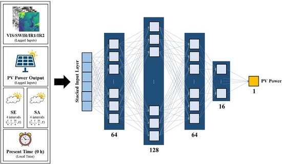
Remotesensing 12 02357 g006
Figure 7. Structure of the deep neural network (DNN) model used in this study showing four hidden layers with 64, 128, 64, and 16 nodes in order of each layer, fully connected to forecast a single PV power output prediction for each hourly timestamp. The various input variables are also included in the diagram to depict the implementation of the input dataset into the input layer of the DNN.
Remotesensing 12 02357 g007
Figure 8. Overview of the main processing steps illustrating the implementation of Section 4.2, Section 4.3 and Section 4.4 on the preprocessed input dataset.
Remotesensing 12 02357 g008
Figure 9. 2 hour (h)- and 1 h-ahead PV forecast results in normalized mean absolute error (NMAE) (%) for each spectral band from COMS and H8 datasets using support vector machine (SVM), artificial neural network (ANN), and DNN models. Solid color bars represent the “Sunlight H” time frame, whereas the overlapping stripe color bars represent the “All H” time frame using identical NMAE scales.
Remotesensing 12 02357 g009
Figure 10. 2 h- and 1 h-ahead PV forecast results in NMAE (%) for each spectral band from COMS and H8 datasets using SVM, ANN, and DNN models based on setup 2.
Remotesensing 12 02357 g010
Figure 11. Monthly accumulated precipitation at each study site where the background area indicates the average monthly precipitation values of the two test sites. Precipitation data are an accumulated sum of the measurements.
Remotesensing 12 02357 g011
Figure 12. Seasonal variation for the 2 h-ahead PV forecast presented by monthly averaged error metrics.
Remotesensing 12 02357 g012
Table 1. Specifications of each test site used in this study.
Test SiteSite LocationData Acquisition PeriodTime Span
135°19′00″ N, 128°20′59″ EApril 2018‒March 20191 year
236°47′47″ N 127°35′40″ E
Table 2. Detailed comparison of the spectral bands for the meteorological satellite images mentioned in this study. Spectral characteristics of GEO-KOMPSAT-2A (GK2A) are also included to show the similarity of the H8 AHI and GK2A Advanced Meteorological Imager (AMI) sensors. The spectral bands used in this study are emphasized in bold text with an asterisk placed next to the band number.
BandWavelength (µm)BandWavelength (µm)
COMS MIH8 AHIGK2A AMI
1Blue0.4600.470
2Green0.5100.510
1 *VIS0.6753 *Red0.6400.640
4VIS0.8600.860
5NIR1.601.38
62.301.61
2 *NIR3.757 *SWIR3.903.83
8WV6.206.24
3WV6.7596.906.95
107.307.34
11IR8.608.59
129.609.63
4 *IR110.81310.410.4
14 *11.211.2
5 *IR212.015 *12.412.4
1613.313.3
Table 3. Evaluation metrics selected to assess the accuracy of PV power forecast results. Data ranges and ideal values are given for each metric.
MetricRangeIdeal ValueFormula
NMAE0 to 10 N M A E = 1 N i = 1 N | ( y i ^ y i ) | C
NRMSE0 to 10 NRMSE = 1 C 1 N i = 1 N ( y i ^ y i ) 2
CC−1 to 11 C C = i = 1 N ( y i μ y i ) ( y i ^ μ y i ^ ) i = 1 N ( y i μ y i ) 2 i = 1 N ( y i ^ μ y i ^ ) 2
Table 4. NMAE results from 2 h-ahead PV power forecast for COMS and H8 datasets using three forecast models in “Sunlight H” and “All H” time frames (bold text indicates the lowest NMAE for each forecast model).
DataModelSunlight H NMAE (%)All H NMAE (%)
VISSWIRIR1IR2VISSWIRIR1IR2
Site 1 COMSSVM6.136.075.915.884.634.474.434.44
ANN5.595.935.765.894.154.264.144.34
DNN5.345.455.345.303.533.813.603.62
Site 1 H8SVM5.926.286.206.184.424.674.584.57
ANN5.575.835.795.844.164.264.344.32
DNN5.125.525.345.393.583.763.893.70
Site 2 COMSSVM6.206.396.396.384.835.084.654.66
ANN5.756.176.006.064.204.654.554.82
DNN5.555.936.096.033.944.044.294.13
Site 2 H8SVM5.966.156.276.334.524.784.734.75
ANN6.336.566.556.574.334.474.754.64
DNN5.736.266.276.283.914.204.544.49
Table 5. NMAE results from 1 h-ahead PV power forecast for COMS and H8 datasets using three forecast models in “Sunlight H” and “All H” time frames (bold text indicates the lowest NMAE values for each forecast model).
DataModelSunlight H NMAE (%)All H NMAE (%)
VISSWIRIR1IR2VISSWIRIR1IR2
Site 1 COMSSVM4.054.074.054.053.323.143.033.04
ANN3.703.683.643.682.652.502.622.58
DNN3.593.563.703.512.252.352.362.32
Site 1 H8SVM4.494.514.474.473.273.413.323.33
ANN3.823.903.983.972.802.892.892.90
DNN3.583.653.833.782.432.532.592.53
Site 2 COMSSVM4.234.534.504.463.453.463.323.31
ANN3.813.763.843.892.712.582.682.61
DNN3.573.693.683.732.282.222.272.31
Site 2 H8SVM4.624.604.634.663.153.423.403.39
ANN3.954.094.194.212.722.913.033.06
DNN3.663.653.843.922.352.462.562.52
Table 6. NRMSE results from the PV forecast for COMS and H8 datasets using the DNN model in “Sunlight H” and “All H” time frames.
Forecast HorizonTest SiteDataSunlight H NRMSE (%)All H NRMSE (%)
VISSWIRIR1IR2VISSWIRIR1IR2
2 h-AheadSite 1COMS8.65 *9.168.998.897.07 *7.667.317.36
H88.42 *9.238.998.967.17 *7.717.787.36
Site 2COMS9.56 *10.1210.139.968.00 *8.288.478.36
H89.81 *10.6010.4110.427.92 *8.748.918.93
1 h-AheadSite 1COMS6.076.036.246.034.78 *4.905.084.92
H85.96 *6.146.276.264.94 *5.075.195.12
Site 2COMS6.40 *6.566.526.565.06 *5.135.195.16
H86.40 *6.506.606.675.44 *5.655.685.68
Bold text indicates the lower NRMSE value between COMS and H8 while the asterisk emphasizes the lowest NRMSE values for each dataset per site.
Table 7. Correlation coefficient (CC) results from PV forecast for COMS and H8 datasets using the DNN model in “Sunlight H” and “All H” time frames.
Forecast HorizonTest SiteDataSunlight H CCAll H CC
VISSWIRIR1IR2VISSWIRIR1IR2
2 h-AheadSite 1COMS0.953 *0.9470.9500.9510.964 *0.9580.9620.962
H80.953 *0.9470.9490.9480.963 *0.9580.9590.961
Site 2COMS0.931 *0.9240.9220.9240.948 *0.9410.9390.940
H80.928 *0.9170.9180.9180.947 *0.9360.9340.932
1 h-AheadSite 1COMS0.9770.9770.9760.9770.984 *0.9830.9820.983
H80.978 *0.9760.9760.9760.983 *0.9820.9820.982
Site 2COMS0.970 *0.9690.9700.9690.978 *0.9770.9770.977
H80.969 *0.9690.9680.9670.977 *0.9760.9760.976
Bold text indicates the higher CC value between COMS and H8 while the asterisk emphasizes the highest CC values for each dataset per site.
Table 8. NMAE results from 2 h- and 1 h-ahead PV power forecasts for COMS and H8 datasets using three forecast models (bold text indicates the lowest NMAE values for each forecast model).
DataModel2 h-Ahead NMAE (%)1 h-Ahead NMAE (%)
VISSWIRIR1IR2VISSWIRIR1IR2
Site 1 COMSSVM6.876.886.766.745.265.245.215.22
ANN6.496.696.516.524.894.784.924.83
DNN6.276.346.336.244.444.414.354.49
Site 1 H8SVM6.996.976.876.865.345.295.275.28
ANN6.696.736.636.644.734.704.684.68
DNN6.266.306.296.274.354.354.444.45
Site 2 COMSSVM6.976.916.936.895.295.245.315.28
ANN6.736.806.886.794.834.804.944.80
DNN6.416.596.536.514.574.634.704.60
Site 2 H8SVM7.177.006.986.955.205.215.255.23
ANN6.796.976.997.064.744.734.824.87
DNN6.756.486.606.524.414.614.684.68
Table 9. NRMSE results from PV forecast for COMS and H8 datasets using the DNN model (bold text indicates the lower NRMSE value between COMS and H8 while the asterisk emphasizes the lowest NRMSE values for each dataset per site).
SiteData2 h-Ahead NRMSE (%)1 h-Ahead NRMSE (%)
VISSWIRIR1IR2VISSWIRIR1IR2
Site 1COMS9.819.909.77 *9.787.177.076.98 *7.06
H89.979.77 *9.859.917.026.94 *6.997.04
Site 2COMS9.84 *9.9910.039.967.207.177.247.14 *
H810.3710.0310.159.96*6.99 *7.187.277.29
Table 10. CC results from PV forecast using the DNN model (bold text indicates the higher CC value between COMS and H8 while the asterisk emphasizes the highest CC values for each dataset per site).
SiteData2 h-Ahead CC1 h-Ahead CC
VISSWIRIR1IR2VISSWIRIR1IR2
Site 1COMS0.9230.9230.925 *0.9240.9590.9600.9610.962 *
H80.9160.920 *0.9180.9180.9610.962 *0.9610.961
Site 2COMS0.9160.9160.9150.9150.9560.957 *0.9560.957 *
H80.9060.913*0.9110.9120.958 *0.9570.9570.955
Table 11. Average NMAE results for 2 h- and 1 h-ahead forecasts from both setups organized with respect to the three forecast models (bold text indicates the lowest NMAE values for each model).
ForecastSiteDataAverage NMAE (%)
Sunlight HAll HSetup 2
SVMANNDNNSVMANNDNNSVMANNDNN
2 h- AheadSite 1COMS5.995.795.364.494.223.646.816.556.29
H86.145.765.344.564.273.736.926.676.28
Site 2COMS6.346.005.904.804.554.106.926.806.51
H86.186.506.134.694.554.297.036.956.59
1 h- AheadSite 1COMS4.494.223.643.132.592.325.234.854.42
H84.564.273.733.332.872.525.294.704.40
Site 2COMS4.804.554.103.392.642.275.284.844.63
H84.694.554.293.342.932.475.224.794.60
Table 12. Average NMAE results of individual spectral bands for 2 h- and 1 h-ahead forecasts via the DNN model in both setups (bold text indicates the lowest average NMAE values among the four spectral bands).
Site2 h-Ahead Forecast Results in Average NMAE (%)
Sunlight HAll HSetup 2
VISSWIRIR1IR2VISSWIRIR1IR2VISSWIRIR1IR2
Site 15.615.845.725.754.084.214.174.166.596.656.566.55
Site 25.926.246.266.284.294.544.594.586.806.796.826.79
Site1 h-Ahead Forecast Results in Average NMAE (%)
Sunlight HAll HSetup 2
VISSWIRIR1IR2VISSWIRIR1IR2VISSWIRIR1IR2
Site 13.873.903.953.912.792.802.802.784.834.794.814.83
Site 23.974.054.114.142.642.722.792.784.844.874.954.91
Table 13. Statistical significance of the t-test evaluation in terms of p-value at a significance level of 1%. Two-tailed p-values are used to evaluate the statistical significance of the results (bold text indicates p-values that are below 1% significance level, while the asterisk highlights very low p-values that are near-zero).
ForecastSiteTime Frame (Setup)Two-Tailed p-Value
2 h-AheadSite 1Sunlight H (Setup 1)0.808
All H (Setup 1)0.044
Setup 20.751
Site 2Sunlight H (Setup 1)<0.001 *
All H (Setup 1)<0.001 *
Setup 20.055
1 h-AheadSite 1Sunlight H (Setup 1)0.008
All H (Setup 1)<0.001 *
Setup 20.491
Site 2Sunlight H (Setup 1)0.013
All H (Setup 1)<0.001 *
Setup 20.570
Table 14. Detailed location of automated surface observing system (ASOS) units and their distance to test site locations. The name of each ASOS unit signifies its geographic location. The distance refers to the straight distance between the ASOS unit and the given test site.
Test SiteName of ASOS UnitLocation of ASOS UnitDistance
1Uiryeong35°19′21″ N, 128°17′17″ E5.60 km
2Cheongju36°38′21″ N, 127°16′26″ E22.0 km
Cheonan36°45′44″ N, 127°17′34″ E27.2 km

