DeepInSAR—A Deep Learning Framework for SAR Interferometric Phase Restoration and Coherence Estimation

Abstract

Over the past decade, using Interferometric Synthetic Aperture Radar (InSAR) remote sensing technology for ground displacement detection has become very successful. However, during the acquisition stage, microwave signals reflected from the ground and received by the satellite are contaminated, for example, due to undesirable material reflectance and atmospheric factors, and there is no clean ground truth to discriminate these noises, which adversely affect InSAR phase computation. Accurate InSAR phase filtering and coherence estimation are crucial for subsequent processing steps. Current methods require expert supervision and expensive runtime to evaluate the quality of intermediate outputs, limiting the usability and scalability in practical applications, such as wide area ground displacement monitoring and predication. We propose a deep convolutional neural network based model DeepInSAR to intelligently solve both phase filtering and coherence estimation problems. We demonstrate our model’s performance using simulated and real data. A teacher-student framework is introduced to handle the issue of missing clean InSAR ground truth. Quantitative and qualitative evaluations show that our teacher-student approach requires less input but can achieve better results than its stack-based teacher method even on new unseen data. The proposed DeepInSAR also outperforms three other top non-stack based methods in time efficiency without human supervision.

1. Introduction

Synthetic Aperture Radar (SAR) is a remote sensing technology, which uses active microwaves to capture ground surface characteristics. An Interferometric SAR (InSAR) image a.k.a interferogram is created from two temporally separated single look complex (SLC) SAR images via the point-wise product of one SLC image with the complex conjugate of the other SLC image. Thus each pixel in an interferogram indicates phase difference between two co-registered SLC images. The phase difference encodes useful information including deformation of the earth’s surface and topographical signals, and has been successfully used to obtain the digital elevation model (DEM). InSAR final products are widely used for civil engineering; topography mapping; infrastructure; oil/gas mining; natural hazards monitoring and elevation change detection. In any SAR system, as the satellite circumnavigates earth, SAR sensor launches millions of radar signals toward the earth in the form of microwaves. The SAR image is represented as a SLC image, which is generated based on radar information echoed back from the ground. However, different ground surface compositions have strong impact on these radar signals. Some are reflected away from the satellite, some are absorbed by non-reflective materials and some are reflected back to the satellite. Signal reflections can be noisy resulting in SAR images with strong speckle noise. Furthermore, temporal and spatial variations between two SLC acquisitions, cause decorrelation, which also affects the interferometric phase [1]. Noisy SAR images make the interferometric phase filtering step on their output InSAR image more challenging. It is important to point out that the quality of estimated interferogram has direct importance to the whole processing pipeline. The phase noise will affect all subsequent stages from phase-unwrapping operation to the motion signal modelling [2]. Therefore, restoration of interferometric phase image becomes a fundamental and crucial step to ensure measurement accuracy in remote sensing. In this regard, the coherence map of interferogram is a crucial indicator showing reliability of the interferometric phase [3]. Thus, interferometric phase filtering and coherence estimation are the main focus in this work.

In recent decades, numerous filtering methods have been proposed. BoxCar is a well-known method because it is straightforward. It simply performs a moving average to estimate the variation of local pixel pattern. In Reference [4], the authors show that this average process is a maximum-likelihood (ML) estimator for interferometric phase and coherence when all involved processes are stationary. Unfortunately, InSAR images are inherently non-stationary because of changing topography and ground displacement. While BoxCar filter can be useful in a flat area, it is not suitable for areas with high slope. In addition, BoxCar outputs are unsatisfactory due to its strong smoothing behaviour caused by simple averaging. In addition to significant phase and coherence estimation error, it is vulnerable to loss of both spatial resolution and fine details. Other classical filters, such as median filter, 2-D Gaussian filter and multi-look processing, also have similar limitations. Consequently, researchers started addressing the problem of non-stationary filtering for interferometric phase. Generally speaking, their methods can be categorized into two groups according to whether the filtering is done with or without domain transformation.

Lee filter [5] is a classical method working in the original spatial domain. It adopts local fringe morphology modelling with anisotropic filter, which reduces the noise via local statistics and an adaptive window. The authors of Reference [6] introduced an extension of Lee’s method by using a minimum mean squared error estimator to exclude singular pixels within a selected direction. Another statistical optimization framework is proposed in Reference [7], which applies Bayesian estimation in the filtering process. Some adaptive methods are proposed in References [8,9]. Vasile et al. designed an intensity-driven adaptive-neighbourhood method for denoising interferometric phase images [8]. Yu et al. used a low-pass filter along local fringe orientation with an adaptive-contoured-window [9]. In Reference [10] Wang et al. pointed out phase fringe and noise frequency distribution are different, and hence noise can be detected without destroying the fringe signal. There are also some works which estimate maximum posterior probability, as filtered phase image can be obtained by modelling image prior as a Markov Random Field (MRF) [7,11]. However, how to choose appropriate properties as image prior is still an open problem.

Goldstein filter [12] is the first frequency domain method with Fourier transformation. One of its extensions [13] proposed a technique to preserve the signal in low noise (high coherence) areas by estimating dominant component from local power spectrum of the signal, which also adapts to the local direction of fringes. Other improvements to the Goldstein and Baran filters have been proposed by researchers, who tried to obtain more accurate coherence estimation and overcome the original method’s under-filtering issue on low coherent regions [14,15]. A joint method, which uses modified Goldstein and simplified Lee filter, is invented in Reference [16]. This filter particularly focuses on interferometric phase denoising under high dense fringes and low coherent situation. In Reference [17], the authors pointed out that filtering with adaptive multi-resolution technique is also necessary because of different sizes and shapes of the interferogram. It improves the filtering quality on fringes via better frequency estimation and invalid estimation correction. In Reference [18], the authors first proposed a wavelet domain filter in complex domain (WInPF) based on a complex phase noise model. They proved that phase information and noise can be more easily separated in the wavelet domain. The success of WInPF was of a great importance to lots of subsequent work. Reference [2] applied wavelet packets based Wiener filter to further separate phase information in the wavelet packet domain, it achieves superior performance compared to the WInPF filter. In Reference [19], Bian and Mercer proposed undecimated wavelet transform by treating image filtering as an estimation problem. Overall, wavelet-domain filters seem to better preserve a good spatial resolution than other methods and have high computational efficiency. Xu et al. [20] introduced a joint denoising filter via simultaneous regularization in the wavelet domain. Phase discontinuities are well preserved through this joint sparse constraint and iterations.

The idea of non-local filtering is to explore more information from the data itself. In general, images contain repetitive structures such as corners and lines. Those redundant patterns in an image could be analyzed and explored to improve filtering performance. In recent years, many studies deploy non-local techniques for SAR data filtering from amplitude images de-specking [21,22,23] to interferometric phase denoising [3,24,25,26,27], and InSAR stack multi-temporal processing [28,29]. Compared to the aforementioned methods, non-local based methods always achieve state-of-the-art results. Non-local filtering adapts estimation to the local signal behaviour to deal with non-stationary images like previous approaches, but it also takes consideration of the entire image according to the image self-similarity property. The first non-local method applied to interferometric phase filtering was proposed by Deledalle et al. in Reference [21]. Both image intensities and interferometric phase information are used to build a non-local means model with a probability criterion for estimating pixels. NL-InSAR [3] is the first InSAR application to use a non-local approach for the joint estimation of the reflectivity, interferometric phase and coherence map from an interferogram. In Reference [24,30], researchers achieve better results on textural fine details preservation by combining non-local filtering with pyramidal representation and singular value decomposition. A unified framework (NL-SAR) is proposed in Reference [27] as an extension of NL-InSAR, where an adaptive procedure is carried out to handle very high resolution images. It is able to obtain the best non-local estimation with good quality on radar structures and discontinuities reconstruction. Recently, works on extending and modifying existing image restoration algorithms to suit interferometric phase domain achieve very promising performance. In Reference [10], a modified patch-based locally optimal Wiener (PLOW) method is proposed for interferometric phase filtering that achieves on par and better results than non-local means. Another famous algorithm, non-local block-matching 3D (BM3D) also inspired researchers to propose InSAR-BM3D [26], which delivered state-of-the-art results for InSAR phase filtering. The method is not proposed to do coherence estimation specifically. InSAR-BM3D computes the maximum likelihood estimates of coherence via stack-wise averages. Then the estimated coherence is used to determine the threshold at the collaborative filtering step. Hence, the performance is likely affected by the accuracy of the coherence estimation, which highly depends on how stationary of the whole stack is.

Milestone works using Convolutional Neural Network (CNN) have shown their ability to outperform almost all conventional algorithms on different visual related tasks including image restoration. There are also some recent SAR based studies benefited from CNN, including the Fuzzy superpixels based Semi-supervised Similarity-constrained CNN (FS-SCNN) model [31], which uses an ensemble learning technique to achieve superior prediction on PolSAR images classification task. Ma et al. [32] proposed an attention-based graph CNN to improve the SAR segmentation results. In Reference [33], DeepLabv3+ [34], a well-known image semantic segmentation CNN model, is adopted for oil spill identification on SAR images. A direct automatic target recognition (D-ATR) deep CNN based model is proposed in Reference [35] to obtain high accuracy and fast processing for target recognition that outperforms all other conventional methods. These works benefit from CNNs as superior feature extractors on SAR images. Anantrasirichai et al. [36] employ CNNs in the InSAR phase to volcano deformation monitoring via transfer learning from optical images. In this work, we propose our DeepInSAR architecture, which is a new deep learning-based model for SAR interferometric phase restoration and coherence estimation. The model is empowered by a set of state-of-the-art deep learning techniques, relying on suitable phase-oriented solutions. We aim to design a more effective joint phase filter and coherence estimator, by learning from the pre-generated training data. We pre-processed InSAR data into a single tensor to do a multi-modal fusion analysis of both phase and amplitude information. A densely connected feature extractor is used to achieve multi-scale feature extraction and fusion. Two subsequent fully connected CNN perform phase filtering and coherence estimation from extracted features respectively. InSAR phase noise can be considered as zero-mean additive noise. So, we adopt the residual learning strategy, which has been proven by in the literature as effective for removing such type of noise [37]. Meanwhile, pre-activation and bottleneck [38], as well as batch normalization techniques [39], are used to enhance training efficiency and boost the model’s performance. The remainder of the paper is organized as follows. In Section 2, we briefly define our interferometric phase noise model and describe our proposed DeepInSAR architecture in detail, as well as our experimental setup. Section 3 presents quantitative and qualitative comparison with the performances of three other established methods for both simulated and real data. Result analysis is presented in Section 4. Conclusion and future work are given in Section 5.

2. Materials and Methods

2.1. Phase Noise Model

Similar to the classical additive degradation mode in natural image restoration problem, an interferometric phase can also be characterized by:

$${\theta }_y={\theta }_x+v,$$

(1)

which has been validated in Reference [5]. ${\theta }_y$ denotes the noisy observation, ${\theta }_x$ is clean phase component and v is the noise with zero mean and $\sigma$ standard deviation, $\theta x$ and $\sigma$ are independent of each other. It follows a similar definition in the natural image analysis that clean signals are independent from noise signals. Unfortunately, it is not feasible to directly use natural image processing algorithms in interferometric phase domain, because of branch cuts. According to the SAR interferometric phase calculation, the range of interferometric phase is within $[-\pi ,\pi )$, which means that wrapped phase value could jump from negative to positive or positive to negative $\pi$, and they could represent high-frequency motion signals that should be well preserved. Therefore, in this work, we follow the strategy in Reference [10,18] to process the interferometric phase in the complex domain. In other words, the phase noise model could be represented by real and imaginary channels, which are continuous values:

$$\begin{array}{cc}\hfill y_{Real}& =cos\left({\theta }_y\right)=Qcos\left({\theta }_x\right)+v_r=Q{x}_{Real}+v_r\hfill \\ \hfill y_{Imag}& =sin\left({\theta }_y\right)=Qsin\left({\theta }_x\right)+v_i=Q{x}_{Imag}+v_i.\hfill \end{array}$$

(2)

The noisy phase observation ${\theta }_y$ is decomposed into two components $y_{Real}$ and $y_{Imag}$. $v_r$ and $v_i$ are zero-mean additive noise in the real and imaginary parts, and they are independent from the underlying clean phase signals ${\theta }_x$. As analyzed in Reference [10] Q is a quality indicator, which is monotonically changing with coherence level. We designed our filtering network based on the above complex phase model. During training, the network learns to filter both real and imaginary parts and then the estimated clean phase $\tilde{\theta }x$ could be reconstructed from filtered ${\tilde{x}}_{Real}$ and ${\tilde{x}}_{Imag}$ as:

$$\tilde{\theta }x=arctan\left(\frac{{\tilde{x}}_{Imag}}{{\tilde{x}}_{Real}}\right).$$

(3)

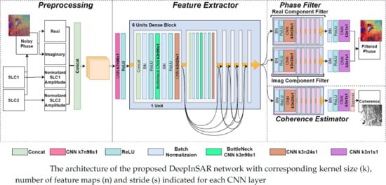
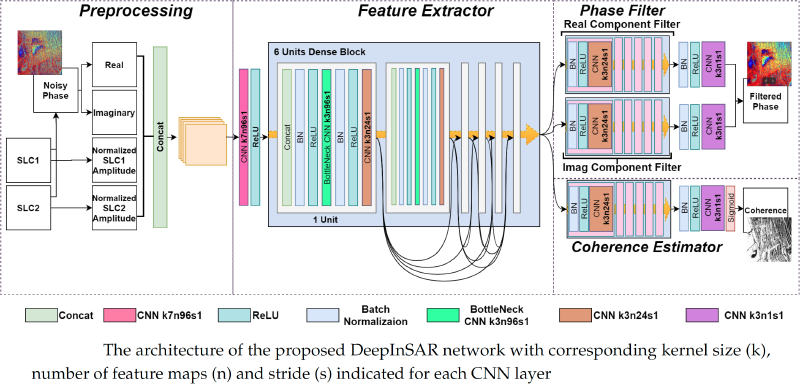
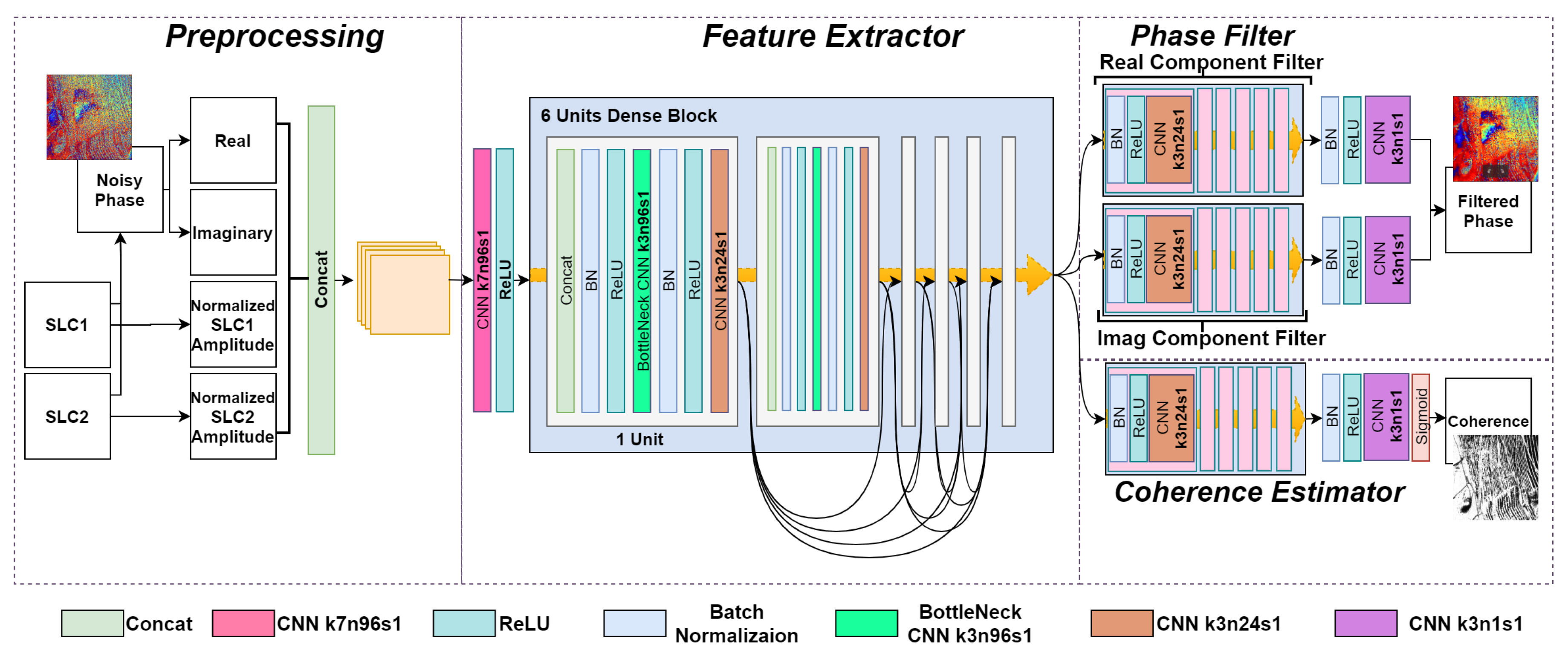
2.2. The Proposed DeepInSAR

In this section, we describe our proposed DeepInSAR in detail. The main goal is to establish and validate the idea of using deep learning method to automate and accelerate both interferometric phase filtering and coherence estimation, which are conducted separately in most of existing approaches. Recently, deep learning studies especially CNNs have been dominating various fields of vision-related tasks. Generally, their excellent performance can be attributed to their powerful feature classification and ability to learn image priors during the training stage. The reasons why we choose to use CNN for InSAR filtering and coherence estimation are (1) CNN is effective for capturing spatial feature characterization with a lot of trained parameters, (2) many achievements in deep learning can be borrowed to benefit better training and generalization, as well as to speed up and improve the output data quality, and (3) powerful GPUs could speed up CNN training and runtime inference. Deep CNN is well suited to be deployed on modern GPUs for parallel computation. All these advantages make deep learning techniques promising for InSAR phase filtering and coherence estimation, where real-time processing and high-quality outcome of large resolution radar images are required.

Figure 1 illustrates the architecture of the proposed DeepInSAR network. At a high-level, our deep model includes multiple modules for handling different subtasks. The amplitudes and their interferometric phases of two SLC SAR images are combined by concatenating into a single tensor during a preprocessing step. The output is subsequently fed into a densely connected feature extractor. Dense connectivity helps extract useful features under different scales and composite multi-scale features are suitable for different end tasks [40]. Two feature to image transformations are achieved by sub-networks performing—(1) phase filtering using residual learning strategy [37] and (2) coherence estimation. The model is expected to learn optimal discriminative functions, mapping from noisy observations to both latent clean phase signals and coherence, by a feed-forward neural network.

2.2.1. Prepossessing of Radar Data

Referring to our noise model in Equation (2), we propose to fully utilize all the information from two SLCs rather than only analyzing interferometric phase. As shown in the Preprocessing Module in Figure 1, the raw input contains two noisy co-registered SLC SAR images $S_1$ and $S_2$. Interferometric phase image I is calculated as:

$$I=(A_{S1}\odot A_{S2})e^{j({\phi }^{S2}-{\phi }^{S1})}=A_I{e}^{j\Delta \phi },$$

(4)

where A is amplitude and $\phi$ is phase. In fact, the phases in SLC images look like random noise from one pixel to another because each pixel is a complicated function of scattering features located on the ground surface. However, interferometric phase $\Delta \phi$ represents phase-difference fringes illustrating changes in distance between ground and satellite antenna, which are valuable information needed for InSAR related applications, but they are often contaminated by noise. Intuitively, we want to incorporate amplitude images, because they usually show recognizable patterns like buildings, mountains, and valleys, which are useful spatial characterizations and hence informative for denoising and coherence estimation. For phase filtering, our proposed DeepInSAR aims to learn a mapping function ${\mathcal{F}}_{oc}:observation\mapsto clean$. As shown in Equation (2), ${\mathcal{F}}_{oc}$ can include noisy $y_{Rea1}$, $y_{Imag}$ and Q as observations. In this work, we further use two SLC’s amplitude value to replace the Q in the observations, because we learn from Reference [41] that coherence magnitude $\left|\gamma \right|$ can be approximated based on two SLC’s amplitude:

$$\left|\gamma \right|=\frac{|{\sum }_{m=1}^M{\sum }_{n=1}^N{A}_{S1}(m,n)A_{S2}(m,n)|}{\sqrt{{\sum }_{m=1}^M{\sum }_{n=1}^N|A_{S1}{(m,n)|}^2{\sum }_{m=1}^M{\sum }_{n=1}^N{\left|A_{S2}(m,n)\right|}^2}},$$

(5)

where $M,N$ represent estimator window size. This widely used coherence estimator shows a potential mapping $(A_{S1},A_{S2})\mapsto \left|\gamma \right|$. Moreover, As mentioned in Section 2, Q is related to $\left|\gamma \right|$. Here we hypothesize that there is a mapping chain $(A_{S1},A_{S2})\mapsto \left|\gamma \right|\mapsto Q$. Hence, instead of using any handcrafted sampling estimator to estimate Q. We proposed to use a deep model to approximate the mapping function ${\mathcal{F}}_{oc}$, in a simplified end-to-end manner by treating both SLC amplitudes together with interferometric phase as input observation to the network. Theoretically, sufficient and well-reasoned input would help the model learn a proper mapping function to estimate latent clean signals more precisely. The same should also support estimating the quality of signals (coherence).

Unfortunately, in real-world SAR image, the range of amplitude values could be extremely broad, that is, from 0 to $1\times {10}^6$, and the scale of the values also varies across different target sites and types of radar sensor. This is one of the reasons why learning-based studies are not pursued for SAR analysis because using uncontrolled amplitude values to train a deep discriminative model is not effective. In general, the learning-based method requires each input dimension to have a similar distribution with low and controlled variance, which has been suggested by many deep learning studies [37,42]. Unnormalized input data can lead to an awkward loss function topology and place more emphasis on certain parameter gradients resulting in a poor training. Hence, for a CNN layer, all the input pixels should be in the same scale. The amplitude values in raw SAR images are not suitable as input data for a deep model. In this work, we introduce an adaptive method to normalize all amplitude values to lie between 0 to 1. The model saturates potential outliers as well as keeps most dynamic changes in the original image without destroying or cutting off any essential ground characteristics.

Knowing that if data roughly follows a normal distribution, the standard Z score of each data point can be calculated as the position of a raw score in terms of its distance from the mean, when measured in standard deviation units [43]. However, SAR amplitude values follow Rayleigh distribution [44] with potential extremes in the distribution tail. Hence, the mean is not statistically robust in our case, and it is easily influenced by outliers. In this study, we apply a modified Z score [45] which estimates Z score based on Median Absolute Deviation (MAD). The MAD value of SLC amplitude A is calculated as:

$$MAD=median\left(\right|A_i-\tilde{A}\left|\right),$$

(6)

where $\tilde{A}$ is the median of the data. Next, we transform the data into the modified Z score domain:

$$A_i^{mz}={\displaystyle \frac{0.6745*(A_i-\tilde{A})}{MAD}}.$$

(7)

$A^{mz}$ represents each pixel’s modified Z score and 0.6745 is the 0.75th quartile of the standard normal distribution, to which the MAD converges. For outlier detection, researchers commonly use absolute values of modified Z scores to threshold the data, where data points with $\left|Z\right|$ score greater than 3.5 are potential outliers and are ignored [45]. In Figure 2, there are 6 SLC amplitude images selected from three real-world datasets captured by TerraSAR-X in StripMap mode [46], with 2 SLCs taken at different time for each stack. By observing their raw amplitude values and histograms as shown in the 1st and 2nd rows of Figure 2, data points are close to Rayleigh distribution as mentioned above. So simply cutting off according to the modified Z score might cause loss of information located on the right tail of high amplitude values. Although logarithm transformation could help us visualize the images better, there is no fixed base number for all images because they might differ by order of magnitude. In our proposed normalization method, we adopt modified Z score as a transformation function to force all values to be close to 0 first and then all potential outliers will be far from 0 and greater than 3.5. To give a standard input data distribution for training the neural network, we apply a hyperbolic tangent $tanh$ non-linear function as:

$$\widehat{A}={\displaystyle \frac{1}{2}}(tanh(\frac{A^{mz}}{7})+1)$$

(8)

to bind all input amplitudes with a controlled variance. A good property of hyperbolic tangent $tanh\left(x\right)$ function is that the input value between −1 to 1 will be enhanced and others will be saturated. In our case, we divide $A^{mz}$ by 7 (two times of 3.5) to make the majority of data points lie between −1 to 1. Then ground characteristics could be potentially enhanced after $tanh$ operations. Secondly, data points with relatively high amplitude are still kept on the right tail, and for those extremely high values, likely outliers, are saturated close to 1. Note that, we further normalize the transformed data to the range [0,1], because we use a Rectified Linear Unit (ReLU) activation for introducing nonlinearity in the CNN to learn complex features. Non-negative input is recommended to avoid saturated neuron at an early training stage when using ReLU activation in the early layers [47]. As shown in the 3rd row in Figure 2, after our proposed data normalization, all amplitude values lie in the range 0 to 1 are properly delivered without losing and breaking essential details. One can also observe this in the 4th row of Figure 2. The final observation $\mathbf{o}$ is a tensor $[y_{real},y_{imag},{\widehat{A}}_{S1},{\widehat{A}}_{S2}]$, and is the input to the proposed DeepInSAR.

2.2.2. Filtering with Residual Learning

Residual learning is designed for solving performance degradation problem on very deep neural networks [48]. In our interferometric phase filtering, we apply a similar idea but without using too many skip-connections within the network. We only create identity shortcuts for predicting the residuals of both real and imaginary channels. Instead of directly outputting the estimated clean components, the proposed model is trained to predict residuals. The model implicitly filters the latent clean signals with hidden operations within the deep neural network. For each of the real and imaginary channels, we have the loss function below:

$$\begin{array}{cc}\hfill \mathcal{L}({\mathbf{W}}_{\mathbf{fe}},{\mathbf{W}}_{\mathbf{real}})& =\frac{1}{2}\left|\right|{\mathcal{R}}_{real}(\mathbf{o};{\mathbf{W}}_{\mathbf{fe}},{\mathbf{W}}_{\mathbf{real}})\hfill \\ & -(y_{real}-x_{real}){\left|\right|}_F^2\hfill \\ \hfill \mathcal{L}({\mathbf{W}}_{\mathbf{fe}},{\mathbf{W}}_{\mathbf{imag}})& =\frac{1}{2}\left|\right|{\mathcal{R}}_{imag}(\mathbf{o};{\mathbf{W}}_{\mathbf{fe}},{\mathbf{W}}_{\mathbf{imag}})\hfill \\ & -(y_{imag}-x_{imag}){\left|\right|}_F^2,\hfill \end{array}$$

(9)

where ${\mathbf{W}}_{\mathbf{fe}}$, ${\mathbf{W}}_{\mathbf{real}}$ and ${\mathbf{W}}_{\mathbf{imag}}$ are the trainable parameters in the model corresponding to feature extractor, real and imaginary channels respectively. For both real and imaginary channels filtering, during the training iterations, our model aims to learn a residual mapping $\mathcal{R}\left(\mathbf{o}\right)\approx y-\frac{y-v}{Q}$ according to our noise model (Equation (1)). Then the clean components can simply be reversed by $x=y-\mathcal{R}\left(\mathbf{o}\right)$. $(y,x)$ represents noise-free training sample (patch) pairs. Residual mapping is much easier to learn than the original unreferenced mapping. It has been shown to output excellent results in many low-level vision image inverse restoration problems such as image super-resolution [49] and image denoising [37]. To the best of our knowledge, we are the first to use residual learning and CNN to do InSAR phase filtering. The model now learns a residual mapping $\mathcal{R}:observations\mapsto residuals$ on real and imaginary channels respectively. Furthermore, it is known that phase noise variance ${\sigma }_{\theta }^2$ could be approximated by coherence magnitude $\left|\gamma \right|$ [41]:

$${\sigma }_{\theta }^2={\displaystyle \frac{{\pi }^2}{3}}-\pi arcsin\left(\right|\gamma \left|\right)+arcsi{n}^2\left(\right|\gamma \left|\right)-{\displaystyle \frac{L{i}_2{\left(\right|\gamma |}^2)}{2}},$$

(10)

where $L{i}_2$ is Euler’s dilogarithm. Our input tensor for phase filtering includes two SLCs’ amplitudes, which correlated to coherence magnitude. Hence, our designed observation input is well-reasoned for predicting phase residuals.

2.2.3. Coherence Estimation

Coherence map is estimated from two co-registered SAR images and is usually used as an indicator of phase quality. Demarcation of image regions based on the degree of contamination (“coherence”) is an important component of the InSAR processing pipeline. 0 coherence denotes complete decorrelation. On the other hand, successful and accurate deformation is measurable with high coherence. Lower quality of interferometry corresponds to decreasing coherence level and increasing level of noise on the phase. Interferometric fringes can only be observed where image coherence prevails. Filtered output is usually combined with coherence map for further processing, because coherence map could tell how much useful signals are potentially within this area. Some of the filtering studies also require coherence map in the filtering process. However, most of them use Maximum Likelihood (ML) estimator (Equation (5)) or its extensions, which are usually significantly biased when using small window sizes. These methods can lose resolution and increase computational cost with large window sizes. Generally speaking, an area on the ground is treated as coherent, when it appears to have similar surface characterization within all images under analysis. However, between two SAR acquisitions, subareas will decorrelate if the land surface is disturbed. Therefore, CNN is a very good candidate to handle this spatial and non-local based analysis, especially on our input o, where almost all necessary information is available for learning the features and capturing mapping functions. During training, the model can learn to capture prior knowledge on all training samples and represent the knowledge as network weights. Intuitively, our method takes a more reliable and robust non-local analysis compared to conventional non-stack based work, which only considers one interferogram. It is also more time efficient than stack-based method because there is no requirement for doing heavy runtime analysis after training is done. In our model, we have a separate module in the proposed DeepInSAR for coherence estimation by using the same features extracted from observations $\mathbf{o}$ as shown in Figure 3. Because coherence lies in the range [0,1], we calculate sigmoid cross entropy loss, given logits obtained from last convolution layer’s output $\mathbf{c}={\mathcal{F}}_{oh}(\mathbf{o};{\mathbf{W}}_{\mathbf{fe}},{\mathbf{W}}_{\mathbf{coh}})$:

$$\begin{array}{c}\hfill \mathcal{L}({\mathbf{W}}_{\mathbf{fe}},{\mathbf{W}}_{\mathbf{coh}})=\mathbf{z}*-log\left(\sigma \left(\mathbf{c}\right)\right)+(1-\mathbf{z})*-log(1-\sigma \left(\mathbf{c}\right))\\ \hfill \mathrm{where}\sigma \left(\mathbf{c}\right)={\displaystyle \frac{e^{\mathbf{c}}}{e^{\mathbf{c}}+1}}.\end{array}$$

(11)

$\mathbf{z}$ is the reference coherence map that can be pre-calculated by any existing coherence estimator in order to generate training dataset for real images.

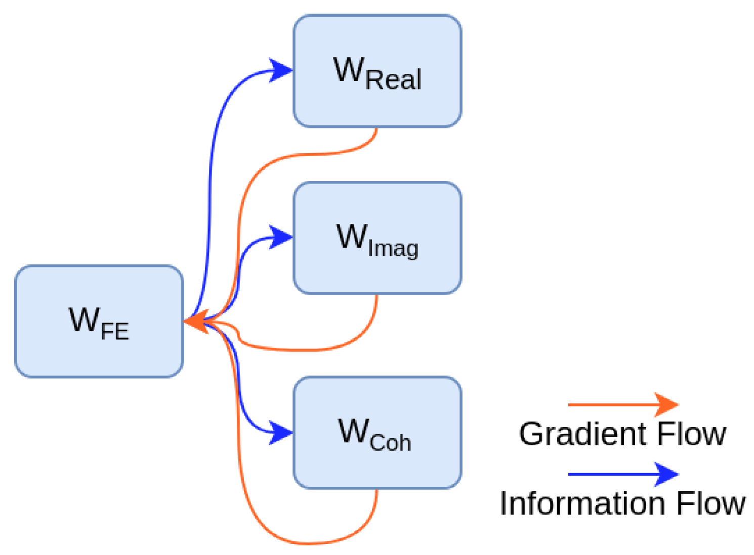
2.2.4. Shared Feature Extractor with Dense Connectivity

Natural images exhibit repetitive patterns, such as geometric and photometric similarities, which provide cues to improve the filtering performance. This concept is also valid for InSAR interferometric phase and SAR amplitude images. However, it should be noted that though, CNNs perform well for visual related tasks, it is known that as CNNs become increasingly deep, both input and gradient information can vanish and “wash out.” Recent work ResNet [48,50] have addressed this problem by building shorter connections between layers close to the input and those close to the output. By doing this, CNNs can be substantially deep but still have accurate performance as well as efficient training. We adopt a dense connected CNN introduced in Reference [40] as a shared feature extractor before the real-imaginary filter and coherence estimator. In the single-look interferometric phase, the latent noise level is related to the coherence magnitude [41]. A shared feature extractor for both phase filter and coherence estimation modules is expected to capture this relationship in latent space because weights in the feature extractor ${\mathbf{W}}_{\mathbf{fe}}$ are updated based on the gradient feedback back-propagated from both phase residual prediction and coherence estimation as shown in Figure 3. During training, the model can encode non-local image prior by updating network parameters according to both phase filter and coherence estimator loss. After training, the model can directly produce filtering and coherence output with a learned discriminative network function without any runtime non-local analysis.

Furthermore, because of the dense connectivity, our feature extractor follows multi-supervision that learns to extract common feature parameters for all related subsequent tasks [39]. In case of dense connectivity, each layer in the feature extractor is connected to every other layer in a feed-forward manner. During gradient back-propagation, each layer’s weight is updated based on all subsequent layers’ gradients [40]. As shown in Figure 1, features extracted by each layer in the feature extractor module of DeepInSAR are based on all preceding layers’ output. At the same time, its own output is passed to all subsequent layers as input. In our network, all feature maps extracted at different depth levels are passed to both phase filter and coherence estimator as a single concatenated tensor. Note that, as per deep CNNs’ working mechanism, early layers extract most detailed and low complexity features with a small perceptual field. With increasing depth, later layers in the feature extractor start extracting high level and complex features with a larger perceptual field. Therefore, a densely connected CNN feature extractor allows each sub-module to perform its own task with multi-scale and multi-complexity features. The proposed DeepInSAR also achieves a deep supervision by allowing each layer in the feature extractor to have direct access to the gradients from both sub-modules. Dense connectivity guarantees the model to get better feature propagation and enables feature reuse and fusion, which is really important for InSAR phase filtering and coherence estimation. In real-world images, ground data sites contain very different scale level characteristics. That is why most existing methods require user-defined window sizes to extract image characteristics. Therefore, all these methods suffer from the inability to choose a generic optimal window size, and fail to automatically generalize to different data sites. In our case, we use a dense CNN based feature extractor to intelligently select the best multi-level features for subsequent modules. The experiments in Section 4 show that our model is capable of generalizing on phase filtering and coherence estimation for different scale features in one image, as well as performing effectively on new site images.

2.2.5. Teacher-Student Framework

Based on our findings, the main reason why deep learning techniques have not been pursued widely in InSAR filtering and coherence estimation so far is the lack of ground truth image data (reference without noise) for training such models. For training our proposed DeepInSAR model, we need image pairs as described in Section 3. However, there is no ground truth for real-world InSAR images. Therefore we introduce a teacher-student framework to make it feasible to train DeepInSAR for real-world images. From the literature, stack-based methods, like PtSel [51], always give reliable results. PtSel is an industry level algorithm for coherence estimation and interferometric phase filtering, which searches similar pixels across a stack of interferograms in both spatial and temporal domains. There are three key steps of PtSel algorithm (Figure 4) to generate the coherence map for a stack of interferograms. Next, the filtering process is replacing each interferograms’ pixel data by the weighted mean of the phase values of its neighbouring pixels, where the weight is the PtSel generated coherence value. Despite the accuracy of stack-based methods, it requires historic SLCs and intensive online parallel searching using a high-end GPU farm, which limits its ability to be integrated into a time-critical InSAR processing chain. The stack-based methods have to wait for several months to collect sufficient data before it can start processing a new site. Although existing stack or non-stack based methods are powerful, most of them require human expert to ensure intermediate output quality because they are incapable of automatically detecting and removing all possible real-world noise patterns from InSAR data.

We introduce a deep neural network to replace the manual pre-processing, that is, feature extraction; and post-processing, that is, quality inspection, with a single intelligent trainable model. Similar to training an object classification neural network model, a large human labeled dataset is required in our approach. Human thus acts as a teacher to teach the model how to classify objects by providing human labeled data. For InSAR phase restoration and coherence estimation, we adopt the PtSel method to create filtered phase images for reference, coherence maps with human tuning and full stack processing to make sure the results are sufficiently reliable. The detail of the PtSel algorithm and its GPU implementation can be found at References [51,52]. In our approach, PtSel with expert supervision becomes the teacher of the proposed DeepInSAR model, which is a student. We are able to demonstrate that, after training, (1) the student DeepInSAR can generate on par or even better results than its teacher method—PtSel, using the same test data sets, (2) our model only requires feed-forward inference on a single pair of SLCs, while PtSel requires more than thirty SLCs; and (3) our model can output filtering and coherence results after a one pass computation, while PtSel requires back and forward tuning processes and needs the phase unwrapping step, which is time consuming.

2.3. Experimental Setup

We compared our method with a number of other non-stack based methods, which can also perform both phase filtering and coherence estimation. They are (1) BoxCar filter, (2) NL-SAR [27] and (3) NL-InSAR [3]. We used publicly available implementations of these methods found in https://github.com/gbaier/despeckCL. Note that all parameters were set, when applicable, as suggested by the authors of the original papers, or else chosen to optimize the performance. We implemented the proposed DeepInSAR using Tensroflow-GPU 1.10; the code is available at: https://github.com/Lucklyric/DeepInSAR. In order to maximize the randomness of the training patch samples, for a given training dataset, the model was trained on randomly extracted image patches with a size of 128 × 128 on the fly [53]. Network parameters were updated using Adam optimizer with a batch size of 64 and 0.001 initial learning rate. The model was trained on two NVIDIA 1080 GPUs for 6 hours with $1.6\times {10}^5$ iterations. To fairly compare the computational time, we executed all methods on the same GPU with an i7-8700K processor and 32 GB RAM. It is worth noting that we built and trained our model using common hyper-parameter settings in our experimental setup because the work presented in this paper is mainly for validating the feasibility of using deep learning techniques to do InSAR phase filtering and coherence estimation. It is expected that more extensive hyper-parameter tuning will further improve the performance of our proposed deep model based on the findings in References [40,49]. We conducted our experiments using both simulated and real-world data to assess the effectiveness and robustness of the proposed model. In this section, we also discuss learning capacity and generalization ability, which are essential criteria for evaluating a learning model.

3. Results

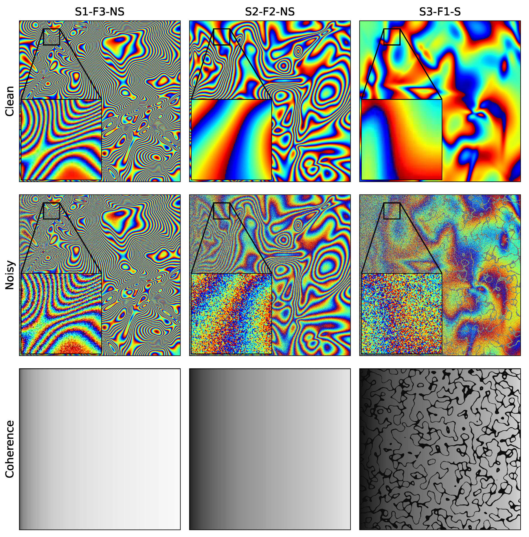
3.1. Results on Simulation Data

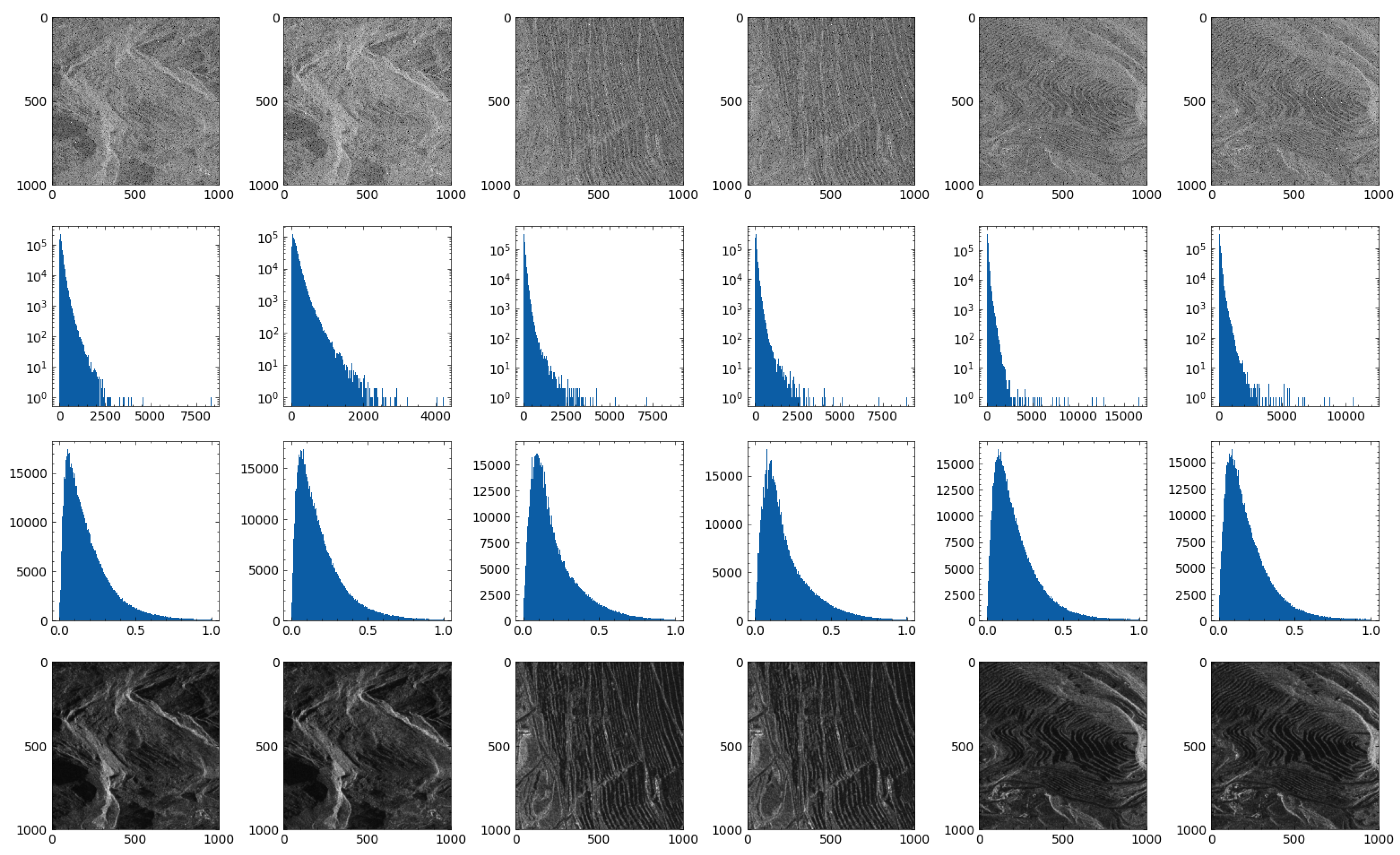
In this section, we present quantitative results using simulated data. Simulated data allows us to evaluate the filtered quality in a controlled environment by comparing with the simulated ground truth. Ground truth is treated as an optimal teacher for training our proposed DeepInSAR; we can objectively demonstrate our model’s capability to learn proper phase filtering and coherence estimation for new simulated testing images, with ground truth available. The simulation strategy is similar to the work for generating the interferometric phase in Reference [26]. Instead of synthesizing a limited known patterns, the additional advantage is to extend the simulation for randomly generated irregular motion signals, ground reflective phenomena, as well as non-stationary noisy conditions. We designed a synthetic InSAR generator to randomly simulate a pair of SLC SAR images with the following procedure:

• Generate first SLC image $S_1$ with 0 phase value. The amplitude value grows from 0.1 to 1 from the left-most column in the image to the right column following a Rayleigh distribution. This leads to a linearly growing of coherence from left to right.
• Generate second SLC image $S_2$ by adding random Gaussian bubbles as synthetic motion signals to the phase. The amplitude value is equal to $S_1$’s amplitude value.
• Add random low-value amplitude bands (less than 0.3) on $S_1$ and $S_2$ to simulate stripe-like low amplitude incoherence areas.
• Generate noisy SLCs $S_1^{noisy}$ and $S_2^{noisy}$ by adding independent additive Gaussian noise v to both real and imaginary channels of $S_1$ and $S_2$.
• Calculate clean and noisy interferometric phase I and $I^{noisy}$.
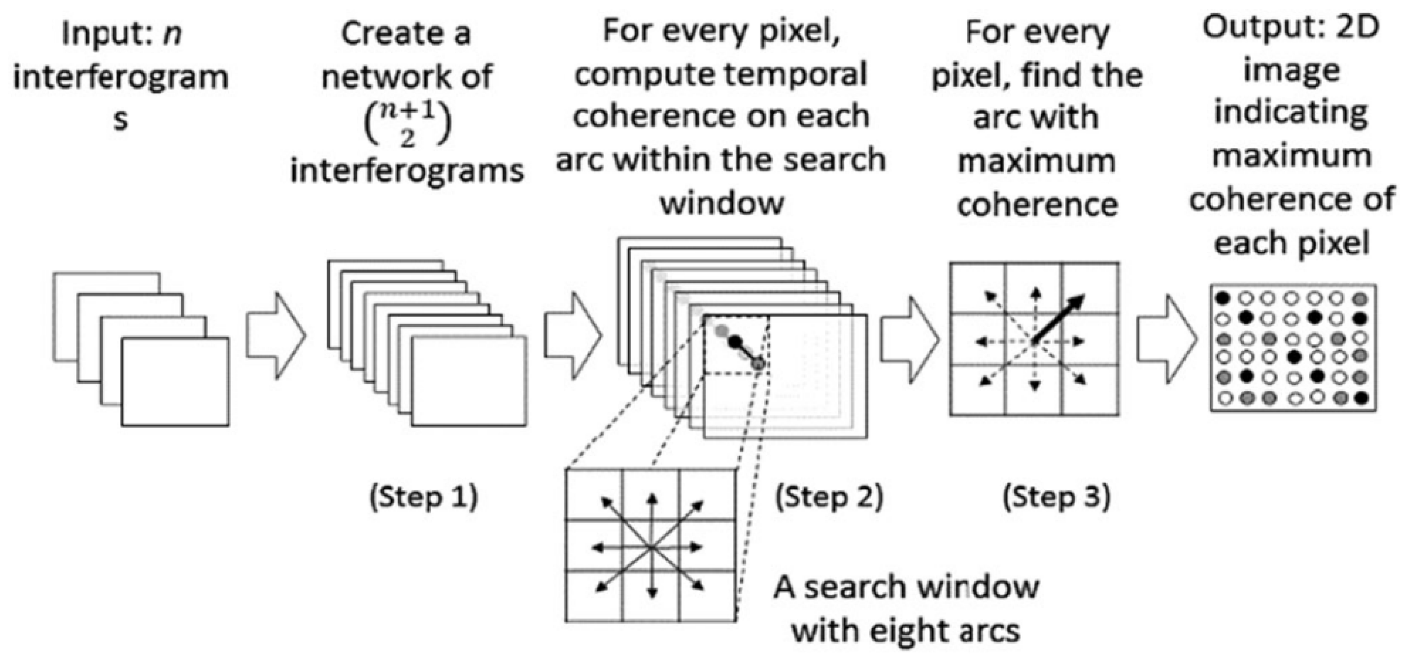
• Calculate ground truth coherence using clean amplitude, phase, and the standard deviation of base noise v.

Our simulated image generator includes a set of parameters for controlling the complexity of the interferometric phase at different distortion levels. We generated 18 different configurations, by combining (1) three base Additive White Gaussian Noise (AWGN) levels of v (S1, S2, S3), (2) three fringe frequency levels of phase fringes (F1, F2, F3), and (3) with or without low amplitude strips (S, NS). For example, the dataset, which has a relatively high level of base noise, and low fringe frequency with low amplitude stripes, is denoted by S3-F1-S. Sample images are shown in the first column of Figure 5. We generated 100 samples with 1000 × 1000 image resolution under each configuration. Half of them were used for training and the rest were for testing. In this experiment, in order to assess the learning capacity and generalization ability of our proposed DeepInSAR model, a single model was trained on all 18 datasets with the noise-free ground truth images (teacher). Because all amplitude stripes and motion signals are randomly generated, all images between training and testing datasets were distinct. Figure 5 shows randomly selected samples from our simulation dataset. Our data generator is inspired by the noise simulation strategy described in Reference [54]. Basically, we simulate speckle noise by adding uncorrelated zero-mean Gaussian random variables to the real and imaginary parts of both synthetic SLCs before multiplying them for interferogram generation. To get the ground truth coherence for the simulated interferogram, we make an empirical mapping to it from the standard deviation of those random variables and the ground truth amplitude. This is because increasing the noise will decrease the coherence, and decreasing the amplitude will also decrease the coherence. In this case, each pixel in the generated interferogram is composed of 4 zero-mean Gaussian random variables with identical standard deviation. The source code of our simulator and full resolution simulated samples used in the experiments are available online at https://github.com/Lucklyric/InSAR-Simulator.

Visual comparisons with BoxCar, NL-InSAR, NL-SAR, and our proposed DeepInSAR methods are presented in Figure 6. Each two rows show the phase filtering and coherence estimation of the three images in Figure 5 respectively, where (a–d) are filtering outputs and (e–h) are coherence estimations of S1-F3-NS, (i–l) are filtering outputs and (m–p) are coherence estimations of S2-F2-NS, and (q–t) are filtering outputs and (u–x) are coherence estimations of S3-F1-NS. Visual inspection on the filtered outputs compared to ground truth clean phase images in Figure 5 shows that our model can preserve phase structural details better than other methods for increasing base noise levels (Figure 6q–t) and frequency of fringes (Figure 6a–d). As we can observe, all methods work fairly well on low-level noise (S1) and low-level fringe frequency (F1) cases. However, with increasing distortion level, all other methods perform rather poorly. The BoxCar filter loses resolution and produces noticeably squiggly artifacts (Figure 6j,r). In particular, when distortion is with high base noise (S3) and high fringe frequency (F3), our model only loses insignificant detail especially in relatively low coherent regions on the left (Figure 6a,q). Although NL-InSAR can guarantee strong noise suppression with detail preservation on high frequency fringes (Figure 6c), it over-smooths the image when phase distortion level keeps increasing (2nd row of Figure 5); fringe structures are washed out when both distortion level and fringe frequency are high (Figure 6k). For coherence estimation, our proposed DeepInSAR is most matched to ground truth (Coherence row in Figure 5). BoxCar and NL-SAR tend to output low coherence on fast moving areas (Figure 6f,h). NL-InSAR and NL-SAR fail to compute correct coherence around low amplitude strips (Figure 6w,x). NL-InSAR also shows inaccurate coherence estimation between the phase jumps (Figure 6h,p).

We also use objective assessment to evaluate the performance of our method. Our test datasets include 18 × 50 = 900 simulated images with noisy and ground truth phase images, as well as corresponding coherence indices. The results obtained from BoxCar, NL-InSAR, NL-SAR and our proposed DeepInSAR are compared. We computed both Root Mean Square Error (RMSE) in radians (

Table 1. Phase Root Mean Square Error (RMSE) (radians) on 18 different types of Simulation dataset. S denotes Gaussian level of base noise and F represents phase fringes frequency. S and NS mean with and without low amplitude strips respectively. Values with bold fonts indicate the best performance.

Phase RMSE (Radians)
Sim Configuration			Methods
			BoxCar	NL-SAR	NL-InSAR	Proposed
S1	S	F1	0.7469	0.8401	0.8373	0.6939
		F2	1.0697	1.2012	0.9572	0.7422
		F3	1.0699	1.2054	1.0354	0.7890
	NS	F1	0.6675	0.7751	0.7088	0.6570
		F2	0.9906	1.1015	0.8284	0.6938
		F3	0.9623	1.1348	0.9138	0.7261
S2	S	F1	0.8409	0.8782	0.9105	0.8091
		F2	1.1252	1.2319	1.0859	0.8854
		F3	1.2096	1.2801	1.1890	0.9593
	NS	F1	0.7863	0.8199	0.8256	0.7715
		F2	1.0567	1.1687	0.9854	0.8297
		F3	1.1251	1.2186	1.0855	0.8785
S3	S	F1	0.9542	0.9332	0.9648	0.9370
		F2	1.1920	1.2657	1.1883	1.0239
		F3	1.3080	1.3430	1.2940	1.1156
	NS	F1	0.8886	0.8672	0.8976	0.8709
		F2	1.1307	1.2203	1.1159	0.9555
		F3	1.2398	1.2927	1.2120	1.0259
Average			1.0202	1.0988	1.0020	0.8536

), and mean Structural Similarity Map (SSIM) between the filtered phase image and noise-free ground truth to quantitatively evaluate the filtering performance (

Table 2. Phase mean Structural Similarity Map (SSIM) on 18 different types of Simulation dataset. S denotes Gaussian level of base noise and F represents phase fringes frequency. S and NS mean with and without low amplitude strips respectively. Values with bold fonts indicate the best performance.

Phase SSIM
Sim Configuration			Methods
			BoxCar	NL-SAR	NL-InSAR	Proposed
S1	S	F1	0.9424	0.8897	0.8566	0.9511
		F2	0.7372	0.6266	0.7723	0.9333
		F3	0.6937	0.5989	0.6888	0.9015
	NS	F1	0.9665	0.8923	0.9505	0.9585
		F2	0.8075	0.7413	0.8887	0.9493
		F3	0.7999	0.7074	0.8117	0.9303
S2	S	F1	0.8898	0.8590	0.8358	0.9122
		F2	0.6624	0.5681	0.6746	0.8647
		F3	0.5150	0.4684	0.5202	0.7976
	NS	F1	0.9221	0.8902	0.9023	0.9312
		F2	0.7357	0.6577	0.7825	0.8966
		F3	0.6152	0.5647	0.6398	0.8527
S3	S	F1	0.8026	0.8168	0.7939	0.8349
		F2	0.5717	0.4989	0.5748	0.7670
		F3	0.3747	0.3555	0.3919	0.6675
	NS	F1	0.8570	0.8722	0.8508	0.8824
		F2	0.6463	0.5736	0.6621	0.8211
		F3	0.4612	0.4375	0.4938	0.7463
Average			0.7223	0.6677	0.7273	0.8666

). RMSE and mean SSIM are also used to assess coherence estimation (

Table 3. Coherence RMSE on 18 different types of Simulation dataset. S denotes Gaussian level of base noise and F represents phase fringes frequency. S and NS mean with and without low amplitude strips respectively. Values with bold fonts indicate the best performance. Values with bold fonts indicate the best performance.

Coherence RMSE
Sim Configuration			Methods
			BoxCar	NL-SAR	NL-InSAR	Proposed
S1	S	F1	0.4360	0.4532	0.3827	0.2125
		F2	0.5418	0.6356	0.3526	0.1838
		F3	0.5321	0.6251	0.3639	0.1850
	NS	F1	0.2119	0.3472	0.1436	0.2045
		F2	0.5458	0.6515	0.1907	0.1633
		F3	0.5444	0.6494	0.2565	0.1564
S2	S	F1	0.4284	0.4522	0.4136	0.2688
		F2	0.4887	0.5564	0.3802	0.2699
		F3	0.4784	0.5463	0.3869	0.2774
	NS	F1	0.2052	0.3303	0.1878	0.2011
		F2	0.4768	0.5664	0.2749	0.2038
		F3	0.4766	0.5600	0.3175	0.2166
S3	S	F1	0.3780	0.3988	0.3834	0.2549
		F2	0.4251	0.4836	0.3726	0.2553
		F3	0.4244	0.4678	0.3805	0.2591
	NS	F1	0.2052	0.2522	0.2086	0.1920
		F2	0.4117	0.4904	0.3116	0.1955
		F3	0.4207	0.4817	0.3419	0.1998
Average			0.4240	0.4971	0.3139	0.2167

and

Table 4. Coherence mean SSIM on 18 different types of Simulation dataset. S denotes Gaussian level of base noise and F represents phase fringes frequency. S and NS mean with and without low amplitude strips respectively. Values with bold fonts indicate the best performance.

Coherence SSIM
Sim Configuration			Methods
			BoxCar	NL-SAR	NL-InSAR	Proposed
S1	S	F1	0.5598	0.5444	0.7150	0.9056
		F2	0.4580	0.2859	0.5979	0.9007
		F3	0.3180	0.1280	0.4455	0.9104
	NS	F1	0.6695	0.7234	0.9497	0.9069
		F2	0.5134	0.4225	0.6767	0.9040
		F3	0.3524	0.2859	0.4318	0.8977
S2	S	F1	0.3621	0.5057	0.6257	0.7349
		F2	0.3100	0.2860	0.4596	0.7649
		F3	0.2340	0.1967	0.2930	0.7508
	NS	F1	0.3061	0.7688	0.8752	0.7864
		F2	0.2422	0.3986	0.4855	0.7584
		F3	0.1756	0.1931	0.1853	0.7994
S3	S	F1	0.2555	0.5082	0.5734	0.6908
		F2	0.2311	0.2952	0.4029	0.7323
		F3	0.1840	0.1728	0.2275	0.7072
	NS	F1	0.1782	0.8209	0.8195	0.7475
		F2	0.1524	0.3910	0.4391	0.7119
		F3	0.1246	0.1552	0.1416	0.7617
Average			0.3126	0.3935	0.5192	0.7984

). Numerical results further confirm our observations that the proposed DeepInSAR significantly outperforms all other methods on most of the 18 different distortion levels. From the simplest (S1-F1-NS) to the most challenging (S3-F3-S) simulation task, all methods have decreasing the performance on both phase filtering and coherence estimation. However, the proposed DeepInSAR has the lest performance degradation and consistently gives better results than the other methods with a total mean of RMSE (radians) 0.8536 and mean SSIM score 0.8666 for phase filtering. The statistical analysis proves that our proposed model can effectively remove the noise and at the same time maintain the structural information effectively. The accuracy of our coherence measurement also shows superior performance with a total mean of phase RMSE 0.2167 and mean SSIM score 0.7984. Coherence computations in all other methods are biased as the data complexity increases, especially when they deal with dense phase fringes (F3) and low amplitudes strips (S).

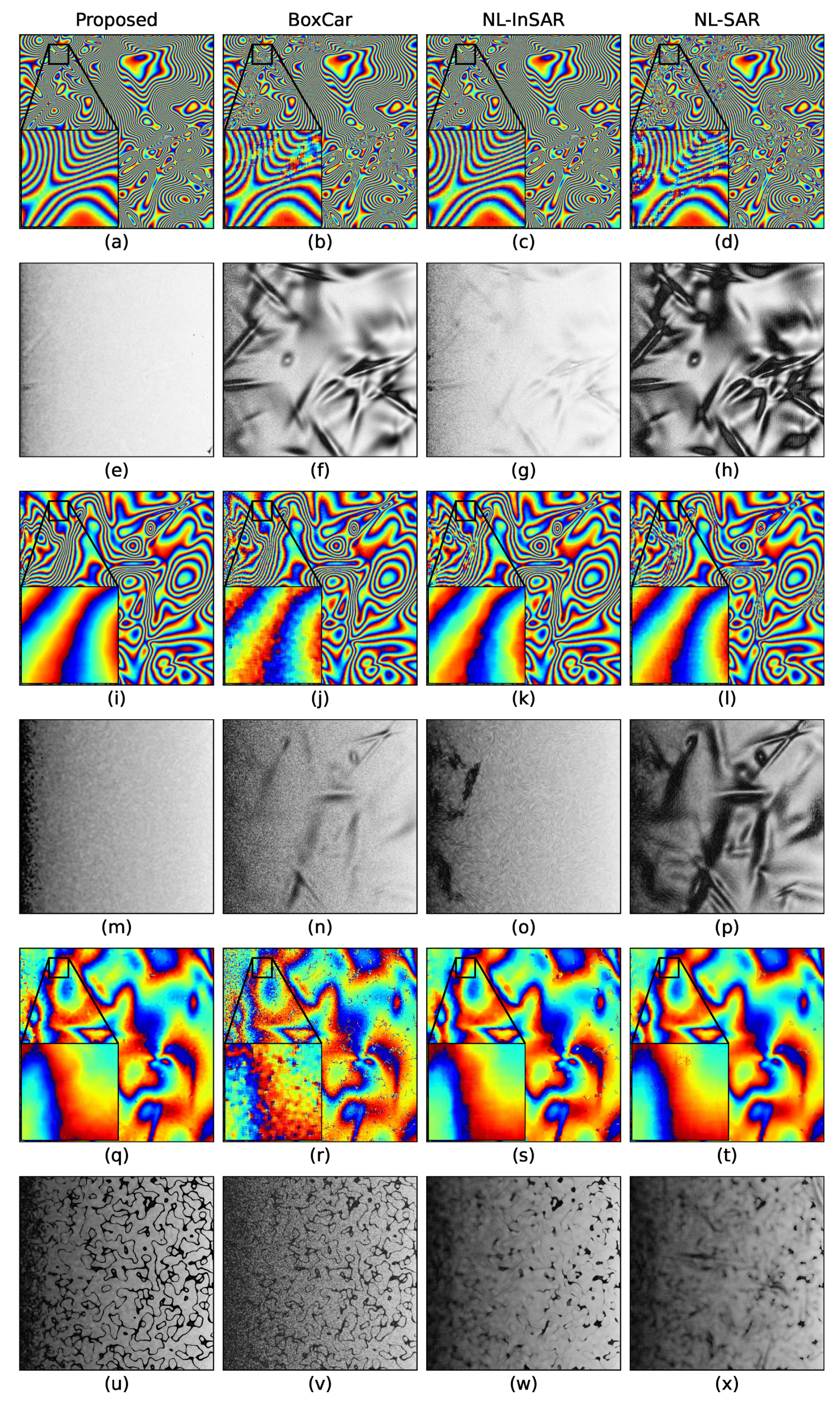
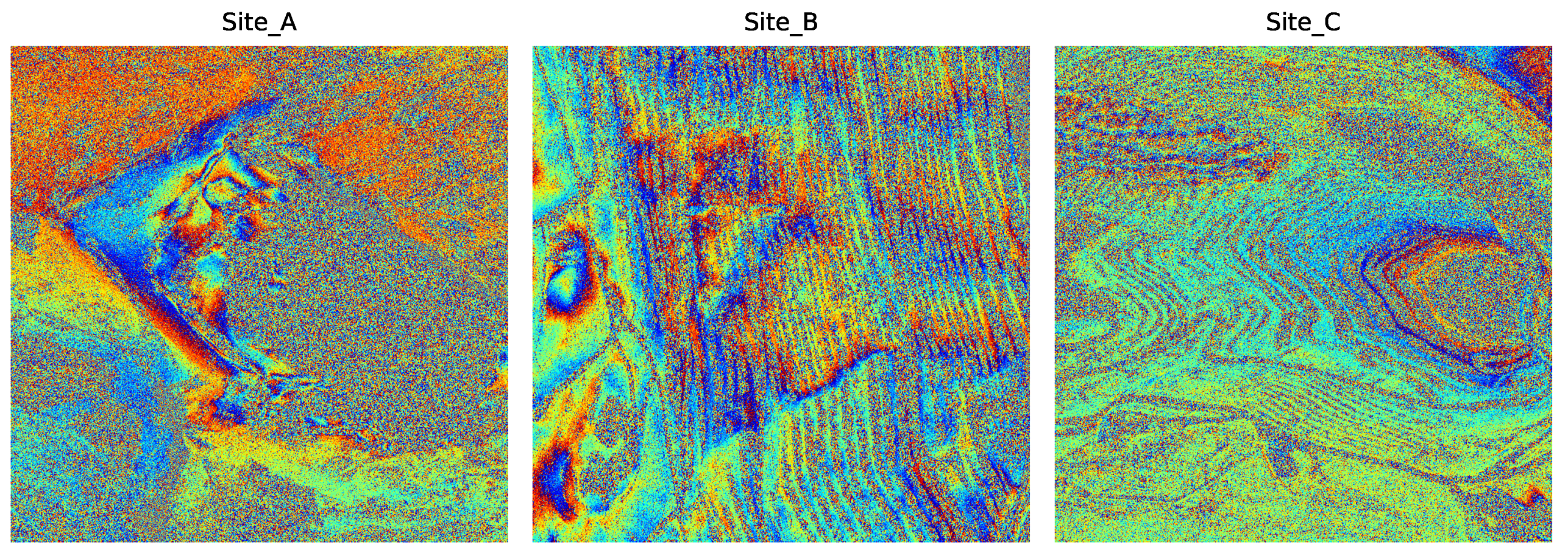
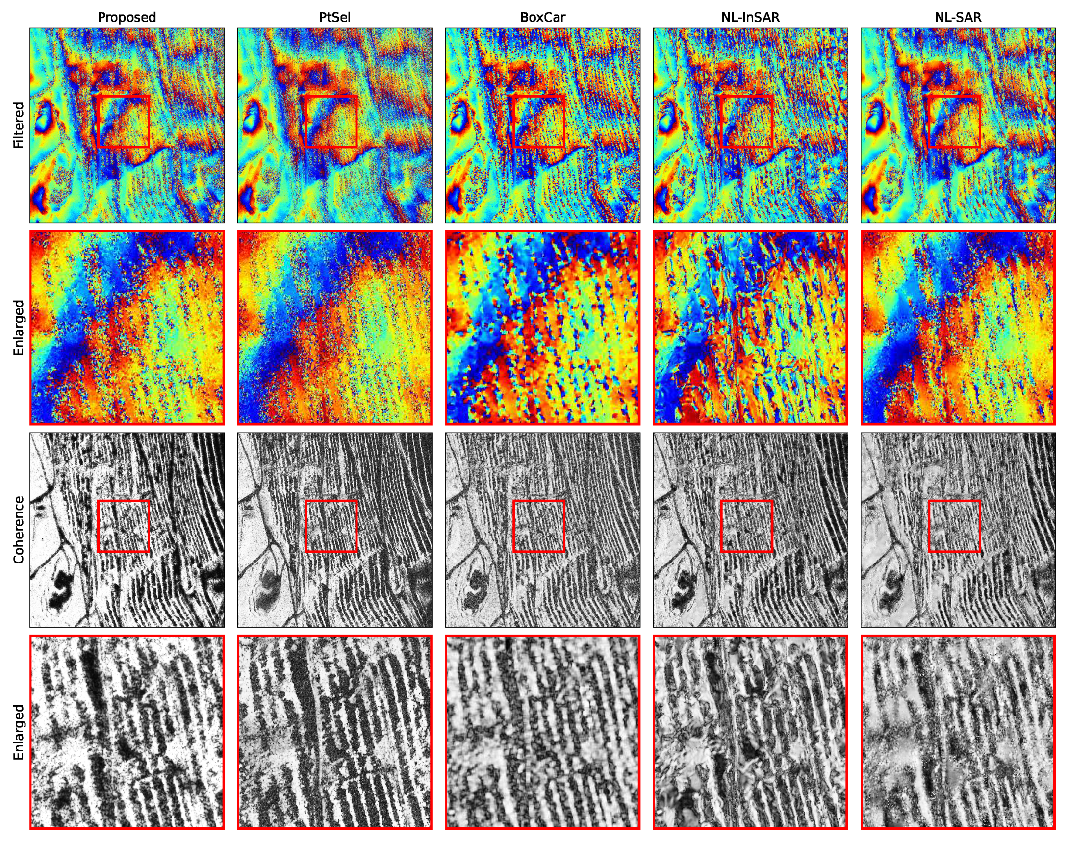
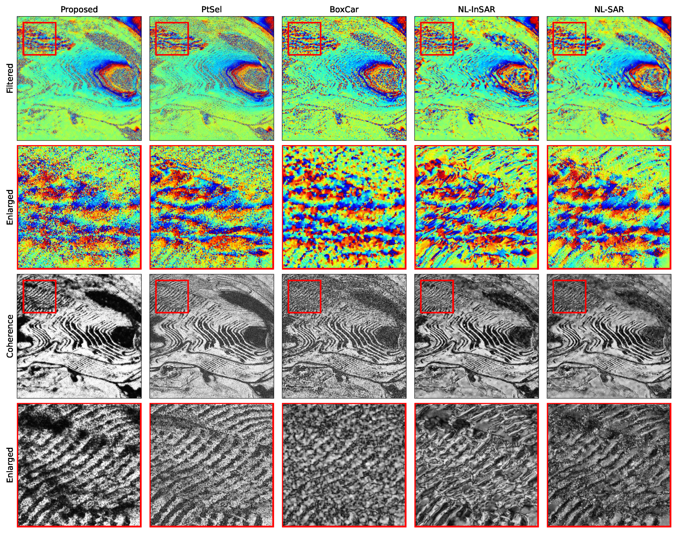
3.2. Results on Real Data

Real complex features and noise patterns cannot be fully replicated by simulation data. However, we can conclude from simulation data experiments that if we can give the model close to clean reference data for teaching DeepInSAR, the model can learn latent mapping from training samples. As mentioned in Section 2.2.5, we use PtSel with expert supervision to generate clean reference phases and coherence maps for three real-world datasets captured by TerraSAR-X in StripMap mode [46]: (1) Site-A—27 SLCs, (2) Site-B—37 SLCs, and (3) Site-C—103 SLCs. We used a cropped version of these datasets with size 1000 × 1000 pixels. For coherence estimation, because the window-based PtSel coherence estimator is biased [51], we applied binary thresholding $0.5$ on PtSel’s coherence output to transform the original regression problem into a classification task. During the inference step, we use coherence estimator’s sigmoid output as the confidence level to represent final coherence magnitude. To demonstrate the generalization ability of the proposed DeepInSAR on real word InSAR data, we trained the model using images from two sites and tested its robustness on the third site. Three representative interferograms selected from each of the three real datasets are shown in Figure 7.

Filtered phases and estimated coherence obtained using BoxCar, NL-InSAR, NL-SAR, PtSel, and our trained DeepInSAR are shown in Figure 8, Figure 9 and Figure 10, which are the outputs of three real sites given in Figure 7. We use qualitative comparison because we do not have noise-free real images for quantity evaluation. The BoxCar filter tends to blur fringe edges in all the visual samples, mainly because of its low-pass behaviour and it under-filters near incoherent areas, which can be easily observed when zooming in. In Figure 8, there appears minor loss of resolution in thin strips (when zoomed in) for the proposed compared to PtSel (stack-based) but is still much better than all other methods that use a single interferogram. NL-InSAR has more stripping artifacts that cause streaks in the phase along incoherence boundaries, which also shown up in its coherence output (Figure 9). It also results in artifacts that follow the benches rather than the fringe lines (Figure 10). NL-SAR can significantly remove the noise, but it also yields over-filtering that breaks some fringes and also merges small scale signals with neighbouring fringes (Figure 8). Overall, though non-local based NL-SAR and NL-InSAR can provide as sharp and visually appealing filtered phase as DeepInSAR on high coherence areas, in medium and low coherence areas, they tend to flatten the phase and create artifacts in highly noisy areas (Figure 8). Both methods have lower overall variance and less blurring than the BoxCar filter, though NL-InSAR has high variance in the estimates between the coherence/amplitude boundaries with streaky artifacts. Our proposed DeepInSAR shows a good balance between noise removal and structural preservation. Regarding to coherence estimation, the proposed DeepInSAR consistently gives better contrast and less spurious high coherence points within the low coherence areas in all the visual samples. It would be easier to be used as the weighting mask for the subsequent InSAR processing e.t. phase unwrapping, compared to other methods. In NL-SAR’s and NL-InSAR’s coherence outputs, there are also artifacts showing high coherence dots in low coherent areas. The limitation is caused by NL-InSAR’s numerical instability algorithm and preferential treatment of amplitude, when the amplitude similarities disagree with the phase similarities. Explanation of NL-InSAR’s weakness is also discussed in Reference [55,56]. Comparing to these non-stack based methods, our DeepInSAR offers both strong noise suppression and detail preservation as well as gives clear high contrast coherence estimation. It performs on par and even better than its stack-based teacher method—PtSel. PtSel’s coherence estimation is biased toward low coherence in the dynamic areas (Figure 8 and Figure 10), because it requires the target remaining stable over a long period of time [51].

4. Discussion

The High-level fringe frequency indicates fast-moving areas on the ground. These areas usually introduce many phase jumps ($-\pi$ to +$\pi$) in the wrapped interferogram. As aforementioned, structural information is one of the most important information that any phase filtering method should preserve. This is because the performance of subsequent InSAR processing, for example, phase unwrapping, is heavily affected by the distorted fringe structure. Many gradient-based phase-unwrapping methods reply on the phase gradients and derivatives, which are types of structural information [10]. As an effective InSAR phase filter, it should preserve the structural details as much as possible [16], and our proposed method demonstrates this capability. For such evaluation, SSIM is a better metric comparing to RMSE for assessing how much structure information has been preserved after filtering. The mean SSIM score (Table 2) indicates that our method preserves excellent details even on highly dense fringes (F3), where all reference methods show decreasing performance as the fringe density increases. Our model shows more noticeable improvement under the SSIM metric than the RMSE metric. It is because RMSE estimates absolute errors and the SSIM provides scores, which focus on the structural similarity. If a filter is over-filtering or breaking the boundary between phase jumps, it may only show insignificant RMSE changes, but will introduce a significant SSIM degradation. Furthermore, if a filter fails to fully suppress the noise signals, the residual noise in the output image will also be reflected more sensitively by SSIM score as in the natural image [57]. This is also the main reason why we use the SSIM metric in the comparisons. Note that, the structural information of coherence is not as important as the filtered phase, because the coherence values are mostly used as a thresholding or weighting metric for subsequent processing. However, we still added SSIM metric for coherence estimation to enrich the experimental analysis. Table 4 shows that the proposed DeepInSAR can predict coherence map most matched to the ground truth. It demonstrates why our method can give high contrast and clear boundaries between extremely low and high coherence areas in both simulation and real site outputs. We believe that a method which can precisely recover the structural information in coherence map must also benefit the subsequent processing with a more detailed and precise coherence indication.

Moreover, in Figure 7, we used three very different real site interferogram examples. Similarly, all test simulation data were generated randomly as described in Section 3.1. Both quantitative and qualitative results confirm that our trained DeepInSAR model generalizes well to new InSAR data without any human supervision or parameter adjustment, which is required by other methods. As an example, when we adjusted the searching window size to a smaller size, NL-SAR and NL-InSAR were able to filter well on those highly dense fringes, but facing under-filtering problem on slow motion areas. During the experiments, we had to manually tune the set of parameters for the reference methods in order to get reasonable results. Their coherence estimators also have similar limitations. In comparison, our proposed model’s coherence output is closest to the ground truth in all different distortion cases. For instance, all three referenced methods tend to give better results when using (1) a small window size on highly dense fringe areas but (2) need a large window size on low frequency motion. There is no fixed size, which works for all 18 simulated distortion levels. However, we show that our learning based DeepInSAR works well for all 18 simulated datasets with a single trained model. It has successfully learned the mapping from noisy observations (18 different distortions) to latent clean signals and coherence magnitudes, when we give it proper training samples to explore. Using densely connected feature extractor gives DeepInSAR the ability to intelligently handle multi-scale signal characteristics with a single model. Since the simulated signal patterns are random, therefore simulated motion patterns, noise conditions and low reflective strips, are irregular among all training and testing images. The evaluation output from the test dataset shows that our trained model does not suffer from the over-fitting issue and only shows a small generalization error, which however has not affected its better performance. It learns well from the teacher and the model can be generalized to new InSAR data. From the operational point of view, NL-InSAR has large amount of artifacts that it produces in the phase and coherence. There are many instances where it does a good job, but in an industrial setting reliability is more important. NL-SAR is better in terms of reliability, but much worse in terms of resolution and is therefore also not an efficient option. The proposed DeepInSAR balances well on noise reduction and fringe preservation. At the same time, it gives a high level of bi-modality in the coherence estimates between the incoherence and coherent pixels.

Furthermore, besides the superior performance compared to other non-stack methods, under a teacher-student framework, DeepInSAR can achieve results comparable to or better than its teacher method with a learned discriminating neural network. The PtSel algorithm (teacher) has several limitations—(1) It relies on temporal information, which means that non-local linear motion can make it hard to pick a neighbourhood suitable for all interferograms, causing under-filtering in these areas. As a result, the algorithm has to wait for many more days of sufficient data before starting the process; (2) It has bias toward filtering results—PtSel looks for similar nearby pixels to perform filtering. If it does not find enough of such pixels, then the filtering is toward averaging, giving worse result compared to another pixel which can find lot of similar neighbours. PtSel’s filtering and coherence output is regarded as state-of-the-art in the literature, but it fails to give optimal output across the test input image because of its biased adaptive kernel estimation. On the other hand, the proposed DeepInSAR successfully distills the knowledge from training samples and generalizes the model to new unseen InSAR images with a simple feed-forward inference, without any human expert supervision, or intensive online searching on a stack of interferograms as required by PtSel. Our proposed DeepInSAR model captures coherence in the fast-moving areas even better than PtSel and produces excellent delineation in the coherence with better contrast, which helps subsequent stages in the InSAR processing pipeline, that is, when thresholding and weighting are required on the estimated coherence in the phase unwrapping stage. With respect to the average running time (T) in seconds, as seen from

Table 5. Running time T (in seconds) of different methods with image size 1000 × 1000.

	BoxCar	NL-SAR	NL-InSAR	Proposed
T (s)	1.16	12.77	19.36	0.46

, the proposed method requires significant less running time than other non-stack methods because only feed-forward computation is needed after training. After testing different parameter settings (e.g., number of iterations and patch size), reference methods sometimes get better results after running for a longer time. However, it is not always the case, which means that these methods have limited potential of full automation without human intervention. The proposed method shows better results with much faster processing time. It is worth mentioning that PtSel outputs used for training and visual comparison are generated using a Titan XP GPU farm. This is because PtSel requires high-end GPUs for intensive parallel searching on a stack of SLCs (>30). In comparison, our method can run on a consumer level system, and perform filtering and coherence estimation using only two SLCs. Taking filtering, coherence performance and flexibility into consideration, the proposed DeepInSAR is very competitive and suitable for real-world InSAR applications.

Lastly, it is worth mentioning that, in this work, our InSAR simulator is mainly designed for quantitative evaluation and analysis, because there is no ground truth data for real-world images. The proposed simulator can generate randomly composite irregular motion signals, ground reflective phenomena, as well as non-stationary noise conditions with different controlled configurations. It is an ideal scenario for objectively assess our proposed DeepInSAR’s learning capacity and ability of generalization. However, as a data-driven technique, when we want to apply the proposed DeepInSAR framework on real-world InSAR data, we need to make sure the training data distribution is similar to real-world scenarios. Existing simulator is designed to give controlled experimental environments for quantitative analysis, but it is still not able to fully replicate the real-world complex features and noise patterns. That is also the reason why we propose the teacher-student framework, which has been validated to be useful for adapting the proposed DeepInSAR to a real-world phase filtering and coherence estimation pipeline. This is also one of the contributions we would like to highlight. We show the potential benefits in the InSAR industry that the proposed DeepInSAR framework has the ability to transform conventional methods, which might require higher computational resources, more input observations, and human supervision, into a differentiable deep neural network model by learning from their outputs. In future work, we plan to investigate a Generative Adversarial Network (GAN) [58] based InSAR simulator for generating more realistic synthetic data. We believe that it will certainly confirm the operationalization aspect of the proposed DeepInSAR.

5. Conclusions

In this paper, we propose a learning-based DeepInSAR framework to address two important research issues: InSAR phase filtering and coherence estimation, in a single process. Our model works well when using either simulated or real data, under different synthetic distortion and real noisy pattern levels. To quantitatively assess the proposed method, we designed an InSAR simulator, which can generate motions and noise patterns randomly. The proposed DeepInSAR outperforms existing non-stack based methods for both tasks by giving the most matched filtered phase and coherence map comparing to the ground truth data. SSIM scores (0.8666 for phase filtering and 0.7986 for coherence estimation) also show superior DeepInSAR performance that can preserve well the phase fringe structure after filtering, and at the same time gives sharp and clear coherence map. Numerical results show that the proposed DeepInSAR can generalize well on new unseen images once it has been trained, and thus can be applied in various real-world InSAR applications. We also presented a teacher-student training strategy, which allows the proposed DeepInSAR to augment, automate and accelerate existing un-differentiable methods using a differentiable deep neural network. Our trained model can obtain the same or better filtering and coherence estimation results only on a single pair of SLC images compared to its teacher algorithm, which requires a stack of SLCs(>30), achieving significantly higher computational efficiency. Comparing to other non-stack based methods, our model gives most robust results on both filtering and coherence estimation (1) without any human supervision and (2) with real-time performance. In addition, the proposed DeepInSAR gives a high level of bi-modality coherence estimation that nicely distinguishes the incoherence and coherent pixels, which benefits the subsequent phase unwrapping. To the best of our knowledge, the proposed DeepInSAR is the first work that uses deep neural network to perform InSAR filtering and coherence estimation jointly using both amplitude and phase information of only two co-registered SLC SAR images. In future work, we will investigate how well the proposed DeepInSAR framework can benefit subsequent InSAR analytic stages along the processing pipeline.

References

1. Hanssen, R.F. Radar Interferometry: Data Interpretation and Error Analysis; Springer Science & Business Media: Berlin, Germany, 2001; Volume 2. [Google Scholar]
2. Zha, X.; Fu, R.; Dai, Z.; Liu, B. Noise reduction in interferograms using the wavelet packet transform and wiener filtering. IEEE Geosci. Remote Sens. Lett. 2008, 5, 404–408. [Google Scholar]
3. Deledalle, C.A.; Denis, L.; Tupin, F. NL-InSAR: Nonlocal interferogram estimation. IEEE Trans. Geosci. Remote Sens. 2011, 49, 1441–1452. [Google Scholar] [CrossRef]
4. Seymour, M.; Cumming, I. Maximum likelihood estimation for SAR interferometry. In Proceedings of the IGARSS ’94—1994 IEEE International Geoscience and Remote Sensing Symposium, Pasadena, CA, USA, 8–12 August 1994; Volume 4, pp. 2272–2275. [Google Scholar]
5. Lee, J.S.; Papathanassiou, K.P.; Ainsworth, T.L.; Grunes, M.R.; Reigber, A. A new technique for noise filtering of SAR interferometric phase images. IEEE Trans. Geosci. Remote Sens. 1998, 36, 1456–1465. [Google Scholar]
6. Chao, C.F.; Chen, K.S.; Lee, J.S. Refined filtering of interferometric phase from InSAR data. IEEE Trans. Geosci. Remote Sens. 2013, 51, 5315–5323. [Google Scholar] [CrossRef]
7. Ferraiuolo, G.; Poggi, G. A Bayesian filtering technique for SAR interferometric phase fields. IEEE Trans. Image Process. 2004, 13, 1368–1378. [Google Scholar] [CrossRef]
8. Vasile, G.; Trouvé, E.; Lee, J.S.; Buzuloiu, V. Intensity-driven adaptive-neighborhood technique for polarimetric and interferometric SAR parameters estimation. IEEE Trans. Geosci. Remote Sens. 2006, 44, 1609–1621. [Google Scholar] [CrossRef] [Green Version]
9. Yu, Q.; Yang, X.; Fu, S.; Liu, X.; Sun, X. An adaptive contoured window filter for interferometric synthetic aperture radar. IEEE Geosci. Remote Sens. Lett. 2007, 4, 23–26. [Google Scholar] [CrossRef]
10. Wang, Y.; Huang, H.; Dong, Z.; Wu, M. Modified patch-based locally optimal Wiener method for interferometric SAR phase filtering. ISPRS J. Photogramm. Remote Sens. 2016, 114, 10–23. [Google Scholar] [CrossRef] [Green Version]
11. Baselice, F.; Ferraioli, G.; Pascazio, V.; Schirinzi, G. Joint InSAR DEM and deformation estimation in a Bayesian framework. In Proceedings of the 2014 IEEE Geoscience and Remote Sensing Symposium, Quebec City, QC, Canada, 13–18 July 2014; pp. 398–401. [Google Scholar]
12. Goldstein, R.M.; Werner, C.L. Radar interferogram filtering for geophysical applications. Geophys. Res. Lett. 1998, 25, 4035–4038. [Google Scholar] [CrossRef] [Green Version]
13. Baran, I.; Stewart, M.; Lilly, P. A modification to the Goldstein radar interferogram filter. IEEE Trans. Geosci. Remote Sens. 2003, 41, 2114–2118. [Google Scholar] [CrossRef] [Green Version]
14. Song, R.; Guo, H.; Liu, G.; Perski, Z.; Fan, J. Improved Goldstein SAR interferogram filter based on empirical mode decomposition. IEEE Geosci. Remote Sens. Lett. 2014, 11, 399–403. [Google Scholar] [CrossRef]
15. Jiang, M.; Ding, X.; Li, Z.; Tian, X.; Zhu, W.; Wang, C.; Xu, B. The improvement for Baran phase filter derived from unbiased InSAR coherence. IEEE J. Sel. Top. Appl. Earth Obs. Remote Sens. 2014, 7, 3002–3010. [Google Scholar] [CrossRef]
16. Wang, Q.; Huang, H.; Yu, A.; Dong, Z. An efficient and adaptive approach for noise filtering of SAR interferometric phase images. IEEE Geosci. Remote Sens. Lett. 2011, 8, 1140–1144. [Google Scholar] [CrossRef]
17. Cai, B.; Liang, D.; Dong, Z. A new adaptive multiresolution noise-filtering approach for SAR interferometric phase images. IEEE Geosci. Remote Sens. Lett. 2008, 5, 266–270. [Google Scholar]
18. Lopez-Martinez, C.; Fabregas, X. Modeling and reduction of SAR interferometric phase noise in the wavelet domain. IEEE Trans. Geosci. Remote Sens. 2002, 40, 2553–2566. [Google Scholar] [CrossRef] [Green Version]
19. Bian, Y.; Mercer, B. Interferometric SAR phase filtering in the wavelet domain using simultaneous detection and estimation. IEEE Trans. Geosci. Remote Sens. 2011, 49, 1396–1416. [Google Scholar] [CrossRef]
20. Xu, G.; Xing, M.D.; Xia, X.G.; Zhang, L.; Liu, Y.Y.; Bao, Z. Sparse regularization of interferometric phase and amplitude for InSAR image formation based on Bayesian representation. IEEE Trans. Geosci. Remote Sens. 2015, 53, 2123–2136. [Google Scholar] [CrossRef]
21. Deledalle, C.A.; Denis, L.; Tupin, F. Iterative weighted maximum likelihood denoising with probabilistic patch-based weights. IEEE Trans. Image Process. 2009, 18, 2661. [Google Scholar] [CrossRef] [PubMed] [Green Version]
22. Parrilli, S.; Poderico, M.; Angelino, C.V.; Verdoliva, L. A nonlocal SAR image denoising algorithm based on LLMMSE wavelet shrinkage. IEEE Trans. Geosci. Remote Sens. 2012, 50, 606–616. [Google Scholar] [CrossRef]
23. Cozzolino, D.; Parrilli, S.; Scarpa, G.; Poggi, G.; Verdoliva, L. Fast adaptive nonlocal SAR despeckling. IEEE Geosci. Remote Sens. Lett. 2014, 11, 524–528. [Google Scholar] [CrossRef] [Green Version]
24. Chen, R.; Yu, W.; Wang, R.; Liu, G.; Shao, Y. Interferometric phase denoising by pyramid nonlocal means filter. IEEE Geosci. Remote Sens. Lett. 2013, 10, 826–830. [Google Scholar] [CrossRef]
25. Zhu, X.X.; Bamler, R.; Lachaise, M.; Adam, F.; Shi, Y.; Eineder, M. Improving TanDEM-X DEMs by non-local InSAR filtering. In Proceedings of the EUSAR 2014; 10th European Conference on Synthetic Aperture Radar, Berlin, Germany, 3–5 June 2014; pp. 1–4. [Google Scholar]
26. Sica, F.; Cozzolino, D.; Zhu, X.X.; Verdoliva, L.; Poggi, G. InSAR-BM3D: A Nonlocal Filter for SAR Interferometric Phase Restoration. IEEE Trans. Geosci. Remote Sens. 2018, 56, 3456–3467. [Google Scholar] [CrossRef] [Green Version]
27. Deledalle, C.A.; Denis, L.; Tupin, F.; Reigber, A.; Jäger, M. NL-SAR: A unified nonlocal framework for resolution-preserving (Pol)(In) SAR denoising. IEEE Trans. Geosci. Remote Sens. 2015, 53, 2021–2038. [Google Scholar] [CrossRef] [Green Version]
28. Su, X.; Deledalle, C.A.; Tupin, F.; Sun, H. Two-step multitemporal nonlocal means for synthetic aperture radar images. IEEE Trans. Geosci. Remote Sens. 2014, 52, 6181–6196. [Google Scholar]
29. Sica, F.; Reale, D.; Poggi, G.; Verdoliva, L.; Fornaro, G. Nonlocal adaptive multilooking in SAR multipass differential interferometry. IEEE J. Sel. Top. Appl. Earth Obs. Remote Sens. 2015, 8, 1727–1742. [Google Scholar] [CrossRef] [Green Version]
30. Lin, X.; Li, F.; Meng, D.; Hu, D.; Ding, C. Nonlocal SAR interferometric phase filtering through higher order singular value decomposition. IEEE Geosci. Remote Sens. Lett. 2015, 12, 806–810. [Google Scholar] [CrossRef]
31. Guo, Y.; Sun, Z.; Qu, R.; Jiao, L.; Liu, F.; Zhang, X. Fuzzy Superpixels based Semi-supervised Similarity-constrained CNN for PolSAR Image Classification. Remote Sens. 2020, 12, 1694. [Google Scholar] [CrossRef]
32. Ma, F.; Gao, F.; Sun, J.; Zhou, H.; Hussain, A. Attention graph convolution network for image segmentation in big SAR imagery data. Remote Sens. 2019, 11, 2586. [Google Scholar] [CrossRef] [Green Version]
33. Krestenitis, M.; Orfanidis, G.; Ioannidis, K.; Avgerinakis, K.; Vrochidis, S.; Kompatsiaris, I. Oil spill identification from satellite images using deep neural networks. Remote Sens. 2019, 11, 1762. [Google Scholar] [CrossRef] [Green Version]
34. Chen, L.C.; Zhu, Y.; Papandreou, G.; Schroff, F.; Adam, H. Encoder-Decoder with Atrous Separable Convolution for Semantic Image Segmentation. In Proceedings of the European Conference on Computer Vision (ECCV), Munich, Germany, 8–14 September 2018. [Google Scholar]
35. Cui, Z.; Tang, C.; Cao, Z.; Liu, N. D-ATR for SAR images based on deep neural networks. Remote Sens. 2019, 11, 906. [Google Scholar] [CrossRef] [Green Version]
36. Anantrasirichai, N.; Biggs, J.; Albino, F.; Bull, D. A deep learning approach to detecting volcano deformation from satellite imagery using synthetic datasets. Remote Sens. Environ. 2019, 230, 111179. [Google Scholar] [CrossRef] [Green Version]
37. Zhang, K.; Zuo, W.; Chen, Y.; Meng, D.; Zhang, L. Beyond a gaussian denoiser: Residual learning of deep cnn for image denoising. IEEE Trans. Image Process. 2017, 26, 3142–3155. [Google Scholar] [CrossRef] [PubMed] [Green Version]
38. He, K.; Zhang, X.; Ren, S.; Sun, J. Identity mappings in deep residual networks. In Proceedings of the European Conference on Computer Vision, Amsterdam, The Netherlands, 8–16 October 2016; pp. 630–645. [Google Scholar]
39. Ioffe, S.; Szegedy, C. Batch Normalization: Accelerating Deep Network Training by Reducing Internal Covariate Shift. In Proceedings of the ICML 2015, Lille, France, 6–11 July 2015. [Google Scholar]
40. Huang, G.; Liu, Z.; Van Der Maaten, L.; Weinberger, K.Q. Densely Connected Convolutional Networks. In Proceedings of the IEEE Conference on Computer Vision and Pattern Recognition (CVPR), Honolulu, HI, USA, 21–26 July 2017; Volume 1, p. 3. [Google Scholar]
41. Bamler, R.; Hartl, P. Synthetic aperture radar interferometry. Inverse Probl. 1998, 14, R1. [Google Scholar] [CrossRef]
42. Glorot, X.; Bengio, Y. Understanding the difficulty of training deep feedforward neural networks. In Proceedings of the Thirteenth International Conference on Artificial Intelligence and Statistics, Chia Laguna Resort, Sardinia, Italy, 13–14 May 2010; pp. 249–256. [Google Scholar]
43. Shiffler, R.E. Maximum Z scores and outliers. Am. Stat. 1988, 42, 79–80. [Google Scholar]
44. Sun, Z.; Han, C. Heavy-tailed Rayleigh distribution: A new tool for the modeling of SAR amplitude images. In Proceedings of the IGARSS 2008—2008 IEEE International Geoscience and Remote Sensing Symposium, Boston, MA, USA, 7–11 July 2008; Volume 4, p. IV-1253. [Google Scholar]
45. Iglewicz, B.; Hoaglin, D.C. How to Detect and Handle Outliers; ASQC Quality Press: Milwaukee, WI, USA, 1993; Volume 16. [Google Scholar]
46. Pitz, W.; Miller, D. The TerraSAR-X satellite. IEEE Trans. Geosci. Remote Sens. 2010, 48, 615–622. [Google Scholar] [CrossRef]
47. Glorot, X.; Bordes, A.; Bengio, Y. Deep sparse rectifier neural networks. In Proceedings of the Fourteenth International Conference on Artificial Intelligence and Statistics, Ft. Lauderdale, FL, USA, 11–13 April 2011; pp. 315–323. [Google Scholar]
48. Szegedy, C.; Ioffe, S.; Vanhoucke, V.; Alemi, A.A. Inception-v4, inception-resnet and the impact of residual connections on learning. In Proceedings of the Thirty-First AAAI Conference on Artificial Intelligence, San Francisco, CA, USA, 4–9 February 2017; Volume 4, p. 12. [Google Scholar]
49. Timofte, R.; De Smet, V.; Van Gool, L. A+: Adjusted anchored neighborhood regression for fast super-resolution. In Proceedings of the Asian Conference on Computer Vision, Singapore, 1–5 November 2014; pp. 111–126. [Google Scholar]
50. Srivastava, R.K.; Greff, K.; Schmidhuber, J. Highway networks. arXiv 2015, arXiv:1505.00387. [Google Scholar]
51. Reza, T.; Zimmer, A.; Blasco, J.M.D.; Ghuman, P.; Aasawat, T.K.; Ripeanu, M. Accelerating persistent scatterer pixel selection for InSAR processing. IEEE Trans. Parallel Distrib. Syst. 2018, 29, 16–30. [Google Scholar] [CrossRef]
52. Reza, T.; Zimmer, A.; Ghuman, P.; Aasawat, T.K.; Ripeanu, M. Accelerating persistent scatterer pixel selection for InSAR processing. In Proceedings of the 2015 IEEE 26th International Conference on Application-Specific Systems, Architectures and Processors (ASAP), Toronto, ON, Canada, 27–29 July 2015; pp. 49–56. [Google Scholar] [CrossRef]
53. Vicente, T.F.Y.; Hou, L.; Yu, C.P.; Hoai, M.; Samaras, D. Large-scale training of shadow detectors with noisily-annotated shadow examples. In Proceedings of the European Conference on Computer Vision, Amsterdam, The Netherlands, 8–16 October 2016; pp. 816–832. [Google Scholar]
54. Goodman, J.W. Speckle Phenomena in Optics: Theory and Applications; Roberts and Company Publishers: Greenwood Village, CO, USA, 2007. [Google Scholar]
55. Zimmer, A.; Ghuman, P. CUDA Optimization of Non-local Means Extended to Wrapped Gaussian Distributions for Interferometric Phase Denoising. Procedia Comput. Sci. 2016, 80, 166–177. [Google Scholar] [CrossRef] [Green Version]
56. Zhu, X.X.; Baier, G.; Lachaise, M.; Shi, Y.; Adam, F.; Bamler, R. Potential and limits of non-local means InSAR filtering for TanDEM-X high-resolution DEM generation. Remote Sens. Environ. 2018, 218, 148–161. [Google Scholar] [CrossRef] [Green Version]
57. Wang, Z.; Bovik, A.C. Mean squared error: Love it or leave it? A new look at signal fidelity measures. IEEE Signal Process. Mag. 2009, 26, 98–117. [Google Scholar] [CrossRef]
58. Goodfellow, I.; Pouget-Abadie, J.; Mirza, M.; Xu, B.; Warde-Farley, D.; Ozair, S.; Courville, A.; Bengio, Y. Generative adversarial nets. In Advances in Neural Information Processing Systems 27; Curran Associates, Inc.: Red Hook, NY, USA, 2014; pp. 2672–2680. [Google Scholar]
Figure 1. The architecture of the proposed Deep Interferometric Synthetic Aperture Radar (DeepInSAR) network with corresponding kernel size (k), number of feature maps (n) and stride (s) indicated for each Convolutional Neural Network (CNN) layer
Remotesensing 12 02340 g001
Figure 2. Before and after preprocessing: amplitude images selected from three real-world site datasets. From left to right, it shows Site-A (1st and 2nd columns), Site-B (3rd and 4th columns), Site-C (5th and 6th columns) with two samples for each dataset. (1st row) Raw amplitude images after log transformation for better visualization, (2nd row) their corresponding histograms in log, (3rd row) histograms after proposed normalization and (4th row) corresponding normalized images.
Remotesensing 12 02340 g002
Figure 3. Information and Gradient flow between modules.
Remotesensing 12 02340 g003
Figure 4. Illustration of the PtSel method describing the three key steps in order [51].
Remotesensing 12 02340 g004
Figure 5. We use S#-F#-S or S#-F#-NS to name simulation datasets generated using different distortion scenarios: S# denotes Gaussian level of base noise S; F# denotes frequency level of phase fringes F; S and NS mean with or without low amplitude strips respectively. (From left to right) A set of simulated images are selected from S1-F3-NS, S2-F2-NS, and S3-F1-S datasets. First row shows simulated ground truth with clean interferometric phase [ π , π ), second row is the noisy interferometric phase [ π , π )—(Blue: π ; Red: + π ), and third row is coherence (Black: 0; White: 1).
Remotesensing 12 02340 g005
Figure 6. Examples of filtering and coherence estimation results on sample simulation images shown in Figure 5. (ad) are filtering outputs and (eh) are coherence estimations of S1-F3-NS, (il) are filtering outputs and (mp) are coherence estimations of S2-F2-NS, and (qt) are filtering outputs and (ux) are coherence estimations of S3-F1-NS. Visual inspection on filtered outputs from different methods compared to ground truth phase images are given in Figure 5, 1st row. It can be seen that our model can preserve structural details better than others for increasing base noise levels and frequency of fringes (5th row). Our proposed method’s coherence estimation is most matched to ground truth (Figure 5, 3rd row), while other methods tend to predict inaccurate results on areas with highly dense fringes or low amplitude stripes.
Remotesensing 12 02340 g006
Figure 7. Three representative noisy interferograms (Phase) selected from each of the three real datasets; Blue: π ; Red: + π .
Remotesensing 12 02340 g007
Figure 8. Filtered images and coherence maps generated by the reference methods and proposed DeepInSAR trained model for a Site-A image.
Remotesensing 12 02340 g008
Figure 9. Filtered images and coherence maps generated by the reference methods and proposed DeepInSAR trained model for a Site-B image.
Remotesensing 12 02340 g009
Figure 10. Filtered images and coherence maps generated by the reference methods and proposed DeepInSAR trained model for a Site-C image.
Remotesensing 12 02340 g010