Analyses of the Prądnik riverbed Shape Based on Archival and Contemporary Data Sets—Old Maps, LiDAR, DTMs, Orthophotomaps and Cross-Sectional Profile Measurements

Abstract

Analyses of riverbed shape evolution are crucial for environmental protection and local water management. For narrow rivers located in forested, mountain areas, it is difficult to use remote sensing data used for large river regions. We performed a study of the Prądnik River, located in the Ojców National Park (ONP), Poland. A multitemporal analysis of various data sets was performed. Light detection and ranging (LiDAR)-based data and orthophotomaps were compared with classical survey methods, and 78 cross-sectional profiles were done via GNSS and tachymetry. In order to add an extra time step, the old maps of this region were gathered, and their content was compared with contemporary data. The analysis of remote sensing data suggests that they do not provide sufficient information on the state and changes of riverbanks, river course or river depth. LiDAR data sets do not show river bottoms, and, due to plant life, do not document riverbanks. The orthophotomaps, due to tree coverage and shades, cannot be used for tracking the whole river course. The quality of old maps allows only for general shape analysis over time. This paper shows that traditional survey methods provide sufficient accuracy for such analysis, and the resulted cross-sectional profiles can and should be used to validate other, remote sensing, data sets. We diagnosed problems with the inventory and monitoring of such objects and proposed methods to refine the data acquisition.

1. Introduction

River morphology studies, including riverbed analyses, are carried out by researchers in many different fields, as they are crucial for assessing flood risks, maintaining ecological balance and protecting the environment [1,2]. These studies include riverbed shape, which will be described in this paper, velocity of water, transportation and accumulation analysis etc. [3,4]. The riverbed shape may be monitored with the use of classical surveying methods or various remote sensing methods [5]: 3D laser scanning [6] and synthetic-aperture radar (SAR) [7], Light Detection and Ranging (LiDAR) [8] or satellite and aerial imagery [9]. The advance of remote sensing methods brought new quality to the field, allowing for faster inventory of large, remote areas and resulting in voluminous, detailed data sets.

The constant evolution of riverbed shape is an inevitable phenomenon. Changes may be caused by climate, erosion, sediment transportation and accumulation [10], and anthropogenic factors, e.g., the construction of dams and platforms [11] etc. Only by careful environmental management, preceded by a thorough analysis of changeability over time and predicting future patterns, is it possible to effectively develop terrains located in the river’s vicinity [4], preserve their natural character, avoid potential damages and minimise flood risks. Hence, it is crucial to provide regional governing bodies, responsible for water management, with accurate data concerning riverbed changes over time. As river characteristics vary depending on numerous geomorphological, climate and anthropogenic factors, different methods may be implemented, in order to monitor riverbed shapes.

Large river regions are often measured with various remote sensing methods. Such an example can be seen in a research study where the authors analysed an area of over 1000 km², including both the rivers and surrounding terrain in the Zagros belt on the border between Iraq and Iran [12]. They used QuickBird satellite scenes processed with geographic information system (GIS) software. The potential of remote-sensing techniques is also illustrated in the paper [13], concerning land surface dynamics. Another frequently used method is LiDAR [14,15,16]. As there are numerous techniques used in the riverbed analyses, some of the papers focus on the comparison between different methods. One of such studies describes LiDAR with reference to cross-sectional profiles conducted with conventional ground survey methods in the area of forested mountain stream [8]. In this analysis, many profiles based on LiDAR data agreed well with the data obtained via traditional land-survey methods, however, the authors state that also many other profiles were not accurate enough for geomorphic change detection. Mountainous rivers meandering between rocks and woods were described in several different articles. For example, researchers in Czech Republic were studying the Javoří brook in the Šumava Mountains. They created digital terrain models (DTMs) and orthoimages with the use of images taken by the unmanned aerial vehicle (UAV) and structure-from-motion software. In the course of spatiotemporal analyses, they managed to detect changes in the riverbed shape with satisfying accuracy [17]. A similar approach was implemented during the analysis of the riverine landscape of the Belá River in Slovakia [18] and the Little Patuxent River (Maryland, USA) [19]. Terrestrial laser scanning (TLS) is another frequently used method for modelling riverbed shapes in cases of not very extended study sites. Such an approach was implemented, e.g., during the analysis of a portion of the Elbe river in Czech Republic [6]. Another method that can be used during riverbed analyses is mobile laser scanning [20]. There have also been some works published on riverbed models [21] from the territory of Poland.

Floods and floodplains associated with rivers are also the subject of scientific research. Floodplains and potential damage connected with a flood in the study area of north-eastern Romania were modelled with the use of LiDAR [22]. These data allow for improving the accuracy of the flood hazard maps and contributing to the monitoring of flood-prone areas. A similar research concerning the analysis of river course stability in the Pearl River Delta, China [23], was published. The authors used airborne LiDAR and high-resolution images for a fast and large-scale examination of a potential diverging course of the river and monitoring of its physical conditions. Water level changes detection are crucial for the possible prevention of natural disasters. Another interesting paper [24] used unmanned aerial vehicle (UAV) based photogrammetry and heights obtained from Global Navigation Satellite System (GNSS) measurements to evaluate the water level change of Kilim River (Malaysia). These analyses proved that the usage of these two measurement techniques allows for the generation of digital surface models DSMs) to identify water level changes at different tidal phases.

Based on the literature review, there are other methods applicable for the riverbed analyses. They include satellite altimetry or Global Navigation Satellite System-Reflectometry (GNSS-R). Satellite altimetry technique is usually used for monitoring of sea, lake or river surface, in particular for the calibration of hydrodynamic models [25], water level monitoring [26] or as a main driver of flood hazard monitoring [27]. GNSS-R is used for determining the flowrates over rivers [28], inland water and wetlands monitoring [29] or water level measurements [30]. Along with the advances in technology, there is a constant need to revise the usefulness of particular methods and search for an optimal combination of techniques.

Multitemporal analyses of riverbed changes over long time are of crucial importance. For example, the analysis of changes in water channel and floodplain of the lower Yuba River in California, USA was performed over a period of 100 years. This study was mostly based on photogrammetric data and old maps, including a comparison of a digital elevation model (DEM) and planimetric change analysis [31]. A similar study was performed for the Basento River in Southern Italy. The researchers managed to carry out an analysis of the channel changes over 150 years [32]. Another research using different data sources concerns the Calore River in Northern Italy and change detection of its course since 1870. The data were processed using advanced GIS methods [33]. The GIS methodology was also implemented in the analysis of DEMs based on LiDAR point clouds used, in order to detect oxbows and former meanders of three watersheds in Iowa and Minnesota [34].

This article aims at using some of the previously described remote sensing methods and other techniques, in order to evaluate the current state of the Prądnik River in the area of the Ojców National Park. It also investigates the quality of available remote sensing data, airborne LiDAR data and orthophotomaps, in regard to their possible use in the long-term monitoring of narrow rivers. It provides a detailed analysis of the limitations of these remote sensing data and means of improving on that with the use of other survey techniques and old maps. The crucial element of the conducted analysis was taking into consideration the limitations of use of remote sensing data for the objects as narrow as the Prądnik River and placed in mountain areas. These two factors make the use of any remote sensing method difficult, thus indicating the need for a more complex and multi-source analysis of such rivers.

2. Study Area

The Ojców National Park (ONP) is located in the valley of the Prądnik River, near the city of Kraków, in the south of Poland (Figure 1). It was founded in 1956 as the sixth national park in the country. It covers the area of approximately 21.46 square kilometres in the region of Polish Jurassic Highland (pol. Jura Krakowsko-Częstochowska). According to physico-geographical regionalisation, the ONP is located in the Polish Uplands province, the Silesian-Kraków Upland subprovince (Figure 1a), the Kraków-Częstochowa Upland macro-region and the Olkusz Upland mesoregion (Figure 1b) [35]. The general shape of the valley can be seen on a hillshaded DTM (Figure 1d). Characteristic, picturesque limestone formations and mysterious caves of this region have attracted the attention of researchers, sightseers and tourists for over 200 years. These landscape features became one of the main reasons for founding the national park in the neighbourhood of the Ojców settlement [36]. This tiny village was a health resort from 1855 to 1939 where visitors could benefit from exceptional views, richness of nature, healing baths and inhalations available in guesthouses located in the Prądnik River valley [37,38].

The Prądnik is a left-bank tributary of the Vistula River, which is one of the major watercourses in Poland (Figure 1e). The Prądnik is 33.4 km long and its meandering course extends over the north-south distance of 12.2 km in the Ojców National Park. The analysed part of the Prądnik River is approximately 6 km long. The river may be characterised by slight water level and flow variations [39,40]. The Prądnik River was examined in terms of the physicochemical parameters of water springs [41], the contamination of water and sediments with heavy metals [42], the water conditions in the basins [40,43]. The structure of runoff of the Prądnik River in Ojców is dominated by groundwater runoff (90%) [40]. The water levels of the Prądnik River are remarkably stable, with extremely small amplitudes for medium and extreme states. This is a very unique observation for Polish watercourses [44]. The valley was shaped by karst phenomena. Its floor is overlain by young alluvial deposits consisting of sand, gravel, clay, mud, peat and limestone. These sediments have been accumulating in this region for 10 thousand years [36,45]. In the Holocene, sediments of the Prądnik River valley distinguished three types of stratigraphic sequences [46]. In the study area, there are traces of deposits of narrow valleys crossing the elevated part of the upland. Molluscan fauna, in particular types of sediments, reflects the evolution of the environment and the transformation of ecosystems in the Prądnik River valley. The riverbed shape of the Prądnik River was influenced by both natural and anthropogenic processes. Along with the development of industry, mills, fishing sites and roads were created in Ojców and the Prądnik River valley [39]. The Prądnik River valley is affected only sporadically by floods, but they are high in volume and range. During the flood on 18th May 1996, the measured volume of the Prądnik River reached 37 m³/s for one km² of catchment. This is a record value registered for this part of Europe [47]. During that time, a flood wave of 3–4 m was observed, which left the whole of the valley covered in 0.5–0.8 m of water. Such large floods cause morphological changes in the landscape.

The monitoring of natural resources of the Ojców National Park is a subject of various studies [48,49,50,51]. They concern such environmental features as meteorology, air quality, animal habitats, number of species, plants etc. Such activities aim at providing long-term observations of existing patterns, assessing implemented protection measures and preserving natural character of the ONP [52]. Hence, the research concerning detecting changes in the riverbed of the Prądnik over time meets real needs of the Ojców National Park, and may become a valuable component of the aforementioned environmental studies. The shape of the Prądnik River riverbed and its changes have not been studied so far.

3. Materials and Methods—Overview of Available Data, Data Preparation and Data Acquisition

The following flowchart (Figure 2) represents used data sets and methods of processing. In some cases, it shows relations between the data sets and how they were used in the Prądnik riverbed shape analysis.

3.1. LiDAR Based Point Clouds and DTMs of the Prądnik River Valley

During the course of this study, the authors managed to obtain two current airborne LiDAR based point clouds. These products were acquired as .las files that included XYZ coordinates, intensity and the RGB colour of each measured point.

The first point cloud was created during the ISOK program. This program aims to gather the data on the terrain of Poland that could be used for early warning and monitoring of natural disasters, mainly floods, to which the area is susceptible and that in the past has caused a lot of damage. The ISOK data set consists of 3 types of products: a point cloud, a DTM and a digital surface model (DSM) in raster format.

The point cloud was acquired with the use of an airborne platform consisting of an LMS-Q680i RIEGL laser scanner, GPS antenna and a camera installed on a plane flying at about 950 m height. The point clouds were registered with the use of flat surfaces of the rooftops. Four corners measured via the means of tachymetry defined the surfaces. The tachymetric measurements were conducted from two points measured by real-time kinematic GPS (RTK-GPS), one was used as a setup point for tachymetry and the other as a reference. The RGB colours were added to the registered point cloud from an orthomosaic of pictures taken during separate flights. The scanning parameters were as follows: the size of the laser beam on the surface was −0.29 m; the density of the scan was −4.7 pts/m³; the density of points varied, being denser in the direction parallel to the flight route at −0.45 m, and less dense in the perpendicular direction of −0.47 m; the overlap between parallel scanning lines was −35%. The observed density varies within a typical inter-point distance of 0.20 m to 0.45 m. This point cloud was acquired in spring and summer 2013. The accuracy of the registration procedure was reported as 0.25 m.

The second data set was obtained from the Ojców National Park, unfortunately limited metadata were available. The authors of this study managed to find the original order on which a public auction was based. The authorities of the National Park confirm that, even though the acceptance report was lost, the point clouds did fulfil the minimal requirements of the order. The order states that the scanning parameters should be as follows: density of the scan −20 pts/m³, overlap between parallel scanning lines—50%. The survey should be carried out before the 15th of June 2012, the registration should be based on 6 flat surfaces and its accuracy should be of at least 0.20 m. RGB colour was added to the registered point cloud based on the orthomosaic acquired during the same flight. This data set was done for the general inventory of the ONP, most likely in late spring, evidenced by the state of vegetation. The observed density varies within a typical inter-point distance of 0.10 m to 0.35 m.

In addition to the point cloud, the ISOK project provided us with DTM and DSM models developed at a resolution of 1 m. The height accuracy of the DTM model is +/−0.15 m in open spaces and +/−0.3 m in forest areas. On the slopes these accuracy values are even smaller [53]. The height accuracy of the DSM model reaches +/−1 m. Due to the nature of the terrain (forested, steep limestone rocks), the DTM is also characterised by low vertical accuracy (explained later by Figure 8(S 52)) [53]. Based on the point cloud from the Ojców National Park, the DTM and the DSM were also produced with a 0.5 m resolution. According to the order specification, the height accuracy of the DTM and the DSM should be +/−0.3 m (no differentiation per type of surface).

LiDAR based data use Polish cartographic projection PL-1992 (EPSG code: 2180). All other data described in this manuscript were transformed to this projection. The PL-1992 is based on a geocentric ellipsoid GRS-80. For the whole territory of Poland, one zone of the Gauss-Kruger projection is used. The central meridian is 19° with a scale factor of 0.9993 [54].

The characteristics of the data used in the article are described in Table S1 (Table S1—All used data and its characteristic.pdf) in Supplementary Materials.

3.2. Survey of the Prądnik River and its Floodplain

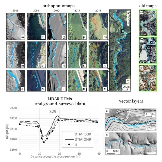
The Prądnik can be described as a narrow, alluvial river with a highly visible floodplain that is surrounded by significantly higher limestone outcrops and stacks, characteristic to this area, partly covered with woods. The valley is 40 m wide in its narrowest part and 180 meters in its widest, also partly covered with trees and buildings. The use of GNSS systems is significantly limited, due to these factors [55,56].

The initial plan for measuring cross-sectional profiles of the river and its floodplain involved the usage of real-time network (RTN) mode with ASG-EUPOS (the network of ground reference stations in Poland) corrections or real-time kinematic (RTK) with corrections from a base located in the nearest area with a good sky visibility. This remote sensing method is the most time-effective due to the fact that it does not require measuring a traverse and can be done with a limited number of personnel. However, its implementation was not possible, due to the field conditions—inadequate satellite coverage above the horizon, which was limited by trees and hills, or a lack of the correction transmission from the system or base station [57]. This proves that current remote sensing methods are severely limited in the areas of narrow mountain rivers. Hence, it was decided to place a traverse along the river and conduct a tachymetric survey from its points, integrated with the GNSS points.

It was not possible to find data on enough survey marks from the Polish national survey mark system, thus 2 pairs (

Table 1. Results of the static Global Navigation Satellite System (GNSS) survey. Coordinates in PL-2000 (zone 7) (EPSG code: 2177).

NR	X [m]	Y [m]	H [m]	dx [m]	dy [m]	dh [m]
1030	5,566,264.041	7,416,480.391	342.569	0.008	0.042	0.008
1029	5,566,118.373	7,416,439.896	341.956	0.018	0.029	0.011
1001	5,563,151.426	7,416,418.191	311.867	0.020	0.030	0.032
1000	5,563,026.745	7,416,439.079	312.653	0.011	0.023	0.042

) of traverse points were measured via static GNSS session [58,59]. The measurements were conducted with 2 Leica GS16 GNSS receivers, collecting the observations synchronically. All of the receivers were mounted on geodetic tripods, the heights of which were reduced to the level of measured points. The elevation angle was set to 10° for all points, each session took two hours with 1 s sampling interval. The points were measured in pairs—a pair at the south end of the traverse was measured first, then a pair in its northern part was surveyed. The GNSS static survey was conducted on the 10th of April 2019. The GNSS measured traverse points were set at the ends of the valley, the only two areas where the satellite coverage was sufficient for a static survey via this remote sensing method.

The post-processing of the measurements was carried out using Leica Geo Office 8.4 software. As a reference, observations form 4 ASG-EUPOS stations (Figure 3) were chosen (KATO—Katowice, KRA1—Kraków, PROS—Proszowice, LELO—Lelów), located 17–57 km from the analysed area.

The post-processing strategy was based on the precise final orbits from the International GNSS Service (IGS) [60] and GPS+GLONASS observations, Hopfield tropospheric model [61], automatic ionosphere model, stochastic modelling and fix ambiguities solutions. The heights (H) in the normal height system were determined with the use of the current quasi-geoid model for the Polish territory—PL-geoid-2011 [54]. The coordinates of 4 reference points and their accuracy are given in Figure 3.

The cross-sectional profiles were measured during two days of a survey session on the 8th and 9th of April 2019. The survey included the measurements of distances and bearings in two series and two positions of the telescope (transits of the scope). Topcon OS total station with a paired standard prism was used in this survey. The accuracy of this instrument is 3” (ISO 17123-3:2001) for a single angle measurement, ±(2 mm + 2 ppm × D) for prism measurements and ±(3 mm + 2 ppm × D) for no prism (ISO 14123-4:2001). The range of this tachymeter is 500 m, thus, it was enough for the purpose of this study. There were 31 traverse points, placed in the average distance of 110 m. Two points at each end of the traverse were also measured with a static GNSS survey, and were used as a reference to the coordinate system. The accuracy of traverse points can be described by horizontal and vertical root mean square error (RMSE) values, which were 43 mm and 13 mm, respectively. The survey of the cross-section profiles was conducted simultaneously with the traverse measurements. Each measured point was surveyed twice with a standard tachymetric method. The average error of each point in XY was 0.043 m, the largest error did not exceed 0.057 m, and the average error in H was 0.013 m and did not exceed 0.016 m.

As a result, 78 cross-section profiles were done, each of 9 points on average, a total of 718 points were measured. The profiles consisted of 1 point on each side of the river representing the water level, at least 1 point in the deepest part of the river and 2–5 points representing the surrounding terrain on each side of the river.

3.3. Orthophotomaps

Orthophotomaps, being another kind of remote sensing data created to provide accurate spatial information on vast areas, were obtained from National Geodetic and Cartographic Resource. The pixel size of the orthophotomaps from 2003, 2009 and 2019 is 0.25 m and from 2017 0.05 m. The orthophotomap from 2003 was created with black and white images, the others are in RGB. The analysed part of the Prądnik River was present on two orthophotomap sheets—M-34-64-B-c-2-3 and M-34-64-B-c-4-1 (signatures in PL-1992 projection).

A vector layer of the river course was created manually for each orthophotomap, using the ArcGIS ArcMap software. The polygons were constructed in the areas where the river was visible. Some areas were covered by tree crowns or shadows, so it was impossible to identify the water course there. The data set from 2019 provided the least data, because the images were taken during spring, when the vegetation significantly limited visibility. It was also difficult to analyse the data set from 2009, as a photogrammetric flight took place during a sunny day, which caused shadows and inconsistencies in contrast. The most data were derived from the orthophotomap from 2003. The approximate length of the vectorised river is presented in

Table 2. Length of the river vectorised on the orthopthotomaps.

Year	Vectorised Length of the River [m]	Percent of the Total Length of the Analysed Part [%]
2003	3230	54.2
2009	2020	33.9
2017	2130	35.8
2019	780	13.1

.

3.4. Old Maps

Old maps presenting the Prądnik River valley were not a frequent subject of research [62]. Old maps that were considered potentially useful are: the Josephine map of Galicia (Josephinische Landesaufnahme) from the 18th century [63], the Map of Ojców surroundings, Edition of the Ojców Bazaar (pol. Mapa okolic Ojcowa Nakład Bazaru Ojcowskiego) from 1907 [64], the Russian and Soviet map in scale 1:84,000 (“two-verst”) from 1914 (Hoвaя Toпoгpaфичecкaя Kapтa 3aпaднoй Poccии, 1:84,000) [65] and the Detailed map of Poland in 1:25,000 scale (pol. Mapa Szczegółowa Polski w skali 1:25,000) from 1935, published by the Military Geographic Institute in Warsaw (WIG) [65,66].

During the research, two additional old maps were considered unsuitable for further analyses of the Prądnik River. These maps are the Map of the Free City of Kraków (pol. Mapa Okręgu Wolnego Miasta Krakowa) from 1833 and the Map of caves in the vicinity of Kraków and Ojców (pol. Mapa jaskiń okolic Krakowa i Ojcowa) from 1929. As a result of the lack of any characteristic objects, it was impossible to georeference them and compare to the current data. However, an approximate location of the riverbed is shown on these maps.

One of the ways to analyse old maps is to compare them by overlaying on the present ones. Problems which can occur while comparing maps from different times are:

• Georeferencing—through ages various maps were created using many cartographic projections with different parameters and accuracy [67]. Some maps were presented with established mathematic assumptions, and some were created without any projection. Georeferencing of this type of maps is possible only by fitting based on points, which have not changed since the maps were created. Sometimes, it is difficult to define such points. Furthermore, deviations on non-cartometric maps are not systematic, thus, it is necessary to use many evenly distributed points in order to perform any georeferencing.
• Interpretation—a map is defined as an ordered and generalised model of reality represented in an arbitrary way using cartographic signs system [68]. Over time, the definitions of symbols have changed. The first complete legend on Polish maps was presented on topographic maps published by the Military Geographic Institute in Warsaw in the 1930s. The first printed maps were created only in one or two colours, so different signs were used to distinguish objects, often very similar to each other and in fact undistinguishable, even within one map sheet. Additionally, a problematic factor is that Polish maps published during the 123 years when Poland was not a sovereign country (from 1795 until the end of the First World War) were created in different countries. Printing techniques, scales, units, sheet formats and used language were different for particular regions occupied by the countries participating in the Partitions of Poland.
• Scale—different scales result in different importance of errors [67]. For example, georeferencing a map at 1:10,000 scale with an RMS error of 100 m would produce an error of 10 mm on this map and can be significant. However, on a map at 1:100,000 scale, the same terrain error results in 1 mm error. This would probably be neglectable as, most likely, the symbols representing objects are larger than the error value.

The first step was the transformation of map scans to one projection based on characteristic points whose location was assumed unchanged through time. The lack of old buildings in the national park induces the decision of choosing less clearly defined objects, such as crossroads, for this task. The reference data was a layer of roads from the Database of Topographic Objects (BDOT10k). The maps were transformed to this projection using the ArcGIS ArcMap software. A transformation method was set as the first order polynomial (affine), which is based on the least-square fitting algorithm. The minimal number of control points for this transformation is 3. Better results are obtained by using more than 3 points distributed evenly around the area of interest. As a result, a raster dataset is scaled, shifted and rotated and receives a new georeference. The next step was the manual vectorisation of the Prądnik River on each map.

The Josephine map of Galicia

The oldest map, the Josephine map of Galicia (Figure 4a,b), was created over the 1779–1783 period for military purposes, and includes lands occupied by Austria after the First Partition of Poland. This map is also called the Mieg map of Galicia. It is a good cartographic source for a historical study of urban development [69]. The map of Galicia was created at 1:28,800 scale. The accuracy of these type of maps is often described as ‘irregular’, as some objects were placed only roughly, and the quality depends on the cartographer’s skills [70]. The survey was based neither on precisely defined triangular points, nor on clearly defined projection. Objects were mapped with an unaided eye and the attention was paid to details which were significant from the military planning perspective, such as communication and transport, castles, churches, rivers [71]. The accuracy of georeferencing of this map can be around 100–200 meters, even less if just a small part of the sheet is georeferenced [72]. The reference points were derived from the Detailed Map of Poland at 1:25,000 scale, which was georeferenced earlier. This process simplified the identification of control points. A total of 8 points were chosen, mostly on characteristic crossroads. The total RMSE is 87.77 m. The river course was vectorised manually.

The Map of Ojców surroundings

The map of Ojców surroundings, Edition of the Ojców Bazaar map (Figure 4c,d) was published in 1907 at 1:100,000 scale. The georeferencing of this map was based on 6 control points located around the river. The reference data was the roads layer of the Topographic Objects Database (BDOT10k). The total RMSE is 27.44 m. The river course was vectorised manually.

The Russian and Soviet “two-verst”

The Russian and Soviet map from 1914 is a “two-verst” map (Figure 4e,f) so it was compiled at 1:84,000 scale. It was the main topographic map for civil and military purposes until 1930s. It was created not only for the Russian territory, but also for Poland, Latvia, Estonia, the Crimea and the Western Caucasus [70]. The map was issued in a two-colour version—black for terrain objects and brown for contour lines. The georeferencing of this map was based on 6 control points located around the analysed part of the river. The reference data was a layer of roads from the Topographic Objects Database (BDOT10k). Total RMSE is 11.05 m. The river course was vectorised manually.

WIG25k

The Detailed Map of Poland at 1:25,000 scale was published by the Military Geographical Institute (WIG) in Warsaw (Figure 4g,h). This map series covered around 50% of the current Polish area and was developed in stages, which causes differences in graphical representation or the reference ellipsoid. The sheet which was used for this study was published in 1935 as a “for tourism” version. It was printed in five colours. The source maps were mainly large-scale maps from the period of the Partitions of Poland [73]. The first step of georeferencing of this map was transforming it into its original cartographic projection. Then, the vector layer that represents the Prądnik was created manually. Later, just the vector layer was spatially adjusted to the PL-1992 projection using control points located on bridges. An affine transformation was used, the total RMSE is 19.80 m.

The Godfryd Ossowski map

As part of the research concerning using old maps to study the shape of the Prądnik riverbed, a map at 1:10,000 scale was found [74]. Unfortunately, the map coverage did not include the whole of the study area, only its south part (Figure 5). This map was created to mark the location of caves in the Prądnik valley. Mills with millraces are also easy to recognise on this map (Figure 5). The publication describing the caves and the map were made by Godfryd Ossowski, one of the fathers of Polish archaeology and the editor of numerous maps [75].

The map was georeferenced using the BDOT10k database and a 1:10,000 topographic map. The affine method was used. RMSE is 8.40 m, which corresponds to an error of 0.84 mm on the map at 1:10,000 scale. This result should be considered satisfactory, given the age of this map. The map was probably made using plane table-based survey.

3.5. Contemporary Vector Data

Due to the small width of the river in the analysed area, only polyline layers can be found in various spatial databases. The polyline layers used during this study are:

• Map of the Hydrographic Division of Poland (MPHP) database. This database was created using the topographic 1:50,000 scale maps and was up to date as of 2010 [76]. Objects are stored in the MPHP database, it is a typical representation of a river network on medium-scale maps [77]. Contrary to other analysed databases, generalised (quantitative and qualitative) objects are stored in the MPHP database.
• The second vector layer was the ONP watercourses (ONPw). This layer was created by the employees of the ONP using manual vectorisation on a high resolution DTM, based on the point cloud from 2012 from the ONP, described in Section 3.1. We used it as a base layer and other layers were compared to it. It is the most current vector layer, and is derived from the most detailed data set.
• The third layer was one of the feature classes of the BDOT10k database—SWRS (pol. sieć wodna - rzeki, strumienie, ang. water network - rivers, streams). The SWRS layer stores river and stream axes. The database was based on the 17 November 2011 Regulation on ‘the topographic objects database and the database of general geographic objects, standards of cartographic studies’ [78]. The BDOT10k database is currently the largest georeferenced Polish database [79]. It was created over many years using various techniques. The analysed fragment of the database is up to date as of 2009 (geometry) and 2013 (attributes). Data in the BDOT10k are in Polish cartographic projection PL-1992 (EPSG code: 2180).
• The next layer (Topo10k92) is not derived from any database, but from the vectorisation of topographic maps at the 1:10,000 scale. These are digital maps but the source layers that were used to render them are not available. Therefore, it was decided to vectorise GeoTIFF files. The vectorisation was based on two sheets: south M-34-64-B-c-4 “Biały Kościół” and north M-34-64-B-c-2 “Skała”. The "Skała" sheet is up to date as of 1996 and “Biały Kościół” sheet as of 2002. It should be noted that these two sheets differ, not only in topicality, but also in technical requirements [80]. The sheet covering the southern part of the study area was issued in accordance with the guidelines of 1999, while the northern sheet was issued in accordance with the guidelines of 1989 [81]. The PL-1992 projection was used during creation of these maps.
• The last layer (Topo10k65), similarly to the previous one, is based on the vectorisation of topographic maps at the 1:10,000 scale, but from an earlier edition. The maps were made in analogue technology. The vectorisation was performed using the WMS layer made available by the Central Office of Geodesy and Cartography in Poland. The study area was covered on two sheets: 163.311 “Wielka Wieś” up-to-date as of 1983–1986 and 163.133 “Skała”, up-to-date as of 1978–1979. These were maps made in accordance with the technical instructions guidelines of 1980 [82]. The maps were made in the PUWG 1965 projection (zone 1) (EPSG: 3120).

4. Results and Discussion

4.1. Analysis of LiDAR Based Data

4.1.1. Point Cloud Comparison

In order to estimate the quality of our two primary remote sensing data sets, point clouds, a cross evaluation was done. Some initial conclusions are listed below:

• None of the data sets could be used for measuring the water floor—topographic LiDAR does not allow for accurate measurements through water, and no other application, for example, bathymetric LiDAR, was used to provide this data, the ISOK data set is incomplete regarding flood monitoring and prediction.
• The ONP point cloud was created relatively fast, within one or two days, judging by the vegetation. It was acquired most likely during late spring, which is unfavourable, due to a large number of deciduous trees that cover the area, thus limiting the density of point cloud representing terrain and creating a large number of blind spots, without any points. However, its short time of creation and relatively high density works in its favour.
• The ISOK point cloud was created during at least two survey series, one in early spring, evidenced by snow cover still visible in the gullies, and the other in mid to late spring, evidenced by the trees and the colour of the grass. Further analysis showed that this point cloud was ‘patched-up’ with other point clouds obtained during many separate surveys, this is evidenced by a significant difference of illumination and difference in the density of the point clouds. Some of those things can be attributed to the fact that images for RGB colour were taken separately, but changes in density and in the vegetation cover are too significant to ignore. As a result, this point cloud is less dense and harder to interpret.
• The ONP point cloud was created with unified density, only changed locally by the amount and type of vegetation. The ISOK point cloud, most likely due to its patched-up origin, consists of square areas of low density, one point every 0.60 m, and areas of high-density, one point every 0.20 m. Additionally, in the ONP, the points are aligned in one direction while in the case of ISOK scan lines change with density. It is worth noting that the metadata do not reflect this information for ISOK. A user might be under the impression that the LiDAR session was done in one set, while following a precisely designed flight plan. No information on changes during scanning or additional data acquisition was given.

Since the point clouds can be viewed as the most recent 3D representation of the valley, we decided to validate them against one another. This was done as follows. The point clouds were loaded into AutoDesk ReCap software. The same, easy to identify objects were localised on both point clouds; these were rooftops, edges of the bridge, corners of the buildings, church tower etc. They were dispersed evenly around the area. Their coordinates were compared, the difference was at 0.34 m at average. Additionally, the −/+ difference was checked, to see if the point clouds were not tilted against each other. This was not observed, the differences were evenly dispersed along the point clouds.

For further processing, the non-terrain elements, trees, buildings, ruins of the castle, and all found artefacts were removed from the point clouds. They were also cut, so that they represent the same parts of the valley and surrounding rock structures. The distances between the point clouds were measured with the use of the CloudCompare software (Figure 6). The initial analysis shows further proper alignment of the point cloud in the vicinity of the road, the only stable, man-made object not extracted for this analysis. The analysis of the road shows that the difference in distance is about 0.10 m—this is fair less than the accuracy of registration for the ISOK point clouds. A total of 65% of surrounding terrain shows similar differences. A total of 15% of differences larger than 0.30 m can be attributed to plant life, more specifically, all grass or small bushes that were impossible to remove. This difference did not exceed 0.50 m. The remaining 20% of differences cannot be attributed to that. This is interesting, since the largest, up to 0.60 m, changes appeared in the east bank of the river (Figure 8(S 12)), smaller, 0.40–0.50 m differences are visible throughout the valley on the east bank and are usually larger in less urbanised areas and on parts of land between the river and the road (this can be either west or east). If terrains with those 20% of differences attributed to the grass are excluded, the models agree with each other well.

4.1.2. Comparison between DTMs and Measured Cross-Section Profiles of the Prądnik River

The authors compared existing spatial data, the ONP and the ISOK based DTMs with measured cross-section profiles, in order to validate their quality and observe if any significant changes occurred between the times when the ISOK data were obtained (2013) and the cross section profiles were measured (2019). A profile analysis was performed as follows. Surveyed points from one profile were connected by a polyline in the ArcGIS ArcMap software (Figure 7a). On this polyline, vertices in 0.5 m sampling were generated. Then, the heights for these vertices were taken from the ONP and the ISOK DTMs (Figure 7b,d). Three height sets—surveyed points and vertices with heights from the DTM ONP and the DTM ISOK models—were compared in Microsoft Excel (Figure 7f). During the field measurements, we tried to keep straight lines for each profile, but this was not always possible (e.g., due to the visibility of surveyed points from the station). Analyses in MS Excel were performed along the section lines connecting the surveyed points.

Figure 8 shows the comparison between several typical profiles with DTMs. It is important to mention at this point that the point clouds, on which the DTMs were based, did not consist of points from the river bottoms. This is due to the fact that airborne laser scanners usually do not penetrate water or create many artefacts when a laser beam passes through this medium. Everything given as a reflection from the water surface and realised as points within a point cloud can be removed via various algorithms, if the inspection of intensity defines those points as false measurements (Figure 8(S 11)). The ISOK DTM is often higher than the ONP DTM in the area of the river bottom, thus, the ISOK represents the riverbanks ending at the water surface and the ONP DTM ends near the water bottom (Figure 8(S 1)). This is most likely due to the different laser scanners used and the different algorithms applied for filtering the noise.

This means that, only differences above a threshold of the water level could be analysed. The DTMs seem to be placed higher in all points measured, this is most likely the result of the technology used during scanning, and also the time of the year when the grass was tall enough to be recorded in a point cloud. This last point is the most significant since the steeper the area gets (less vegetation grows there), the smaller the differences are.

The comparison of models carried out on the profiles shows that in places of large slopes (slopes or rocks), models generated from the point clouds are too smooth. This can result from malfunctioning algorithms for the automatic detection of watercourses. This situation can be observed on the right side of profile 52 (DTM ISOK) and 67 (DTM ONP) and on most profiles on the water-land border (Figure 8). This can be observed more often on the DTM ONP model, despite its greater resolution.

The analysis of profiles allows for concluding that for small rivers, similar to the Prądnik River, waterbed modelling cannot be done accurately by using airborne laser scanning. This applies to both products; point clouds and DTMs. Terrestrial laser scanning could be used for this purpose, but this would require clearing the area, which is impossible due to the National Park regulations of undisturbed nature being left on display. Using UAV with LiDAR or a camera that would allow for structure-from-motion processing could provide sufficient data. However, this would require extensive planning. Airborne LiDAR point clouds, analysed in this study, did not provide enough data, thus, the methodology would have to be customised strictly for this area of study. Another issue is the Polish law, which requires special permissions from the National Park administration and others to perform a UAV flight. This suggests that terrestrial laser scanning would be a reasonable choice for such a survey.

Further profile analysis indicates that, at times, the DTM ONP model shows a wide and flat river bottom (Figure 8(S 11,S 52)). Creating such “lakes” should be described as incorrect. This is one of the problems that may be encountered when using DTMs which were based on airborne laser scanning (ALS) data and created with general purpose algorithms, for hydrological analyses.

In order to give the final check of the quality of the DTMs, a simple statistical analysis was performed. A total of 478 measured points were used (points measured under the water surface were excluded). This was based on calculating the distances between the ISOK and ONP DTMs and measured cross-section profiles. The results are presented in Figure 9 and

Table 3. Statistics based on differences between the ONP and ISOK DTMs and measured cross-section profiles—H (ground truth).

	Point Count	Average [m]	Median [m]	Minimum [m]	Maximum [m]	Bottom Quartile [m]	Upper Quartile [m]	Standard Deviation [m]
DTM:OPN-H	478	0.30	0.27	−0.96	4.51	0.12	0.43	0.42
DTM:ISOK-H	478	0.21	0.16	−0.86	13.00	0.10	0.22	0.67

. This analysis has shown that the ISOK DTM agrees better with measured data, since the difference is significantly smaller than in the case of the ONP. In addition, the ONP DTM is less consistent, which is evidenced by the outliers. This all proves that the ISOK data set, even with previously described problems with density, is better suited for this kind of analysis.

The current shape of the Prądnik River was evaluated based on the measured cross-section profiles and DTMs. The width and depth of the river is presented in

Table 4. Current state of the Prądnik River—width and depth.

	Width [m]	Depth [m]
min	1.53	0.03
max	9.39	1.23
average	3.75	0.32
median	3.34	0.25

. The maximum and minimum width are 9.39 m and 1.53 m. The average width is 3.75 m. In most areas of the river, the depth is lower than 0.3 m, and only in two areas the depth is greater than 1 m. The difference in height between the highest and the lowest point of the river bottom is 31.09 m. The riverbanks are steeper on the west bank.

4.2. Orthophotomaps Analysis

We planned to use the orthophotomaps to perform a detailed analysis of changes of the Prądnik River shape. However, it was impossible to vectorise the whole course of the Prądnik River, because of the high and dense vegetation that covered the river, and shadows which occurred in many parts of the analysed area.

In few places, three or four vector layers were visible (Figure 10, middle row). Apart from those locations, it was possible to compare river shape and detect potential changes. One of the differences can be seen between the second and the third cross-section profile, where the Prądnik River shifted to the west (Figure 10, bottom row). Comparing the DTM ONP from 2012 and the orthophotomap from 2017, this change occurred after 2012 and before 2017, and the shift reaches 3 m. Other significant changes are visible on cross-sections no. 62 and no. 64 (Figure 10, top row). The river course on the orthophotomap from 2003 is similar to the BDOT10k vector layer from 2006, but the orthophotomap from 2009 shows a different course of the river in this location, so the changes occurred between 2006 and 2009. The characteristics and placement of these changes, in the middle of a farmland, suggest that they were manmade. There was a significant change in the shape of the Prądnik River, and the riverbed was displaced by 25 m. In another three areas, the Prądnik River did not change its shape; the displacements of watercourse do not exceed 1 m, and are most likely caused by differences in the water level and the orthophotomap’s geolocation accuracy. There have been no other changes observed in the shape of the watercourse after 2003. The shape on the orthophotomap from 2003 is more irregular and the displacement reaches 1.5 m. In the southern part, we identified an area where the Prądnik changed its shape after 2003, it is less meandering, and these changes reach 1.5 m. In addition, one area where the Prądnik River increased its meanders after 2009 and before 2017 was identified. These changes reach 6 metres. Unfortunately, the area is not visible on the latest orthophotomap. The remaining parts of the river, visible on two or more images, do not show any significant changes.

4.3. Vector Layers Analysis

In this study, a comparison between vector layers representing the Prądnik River was performed. Since the ONP layer was created using manual vectorisation on a high resolution DTM by the Ojcowski National Park employees, it was used as a base layer and other layers were compared to it. The ONP layer is up to date as of 2012.

4.3.1. Current Data Analysis

The MPHP database vector layer was the least accurate of all analysed layers (Figure 11). It was analysed only visually, due to its low accuracy in comparison to the DTM. The reason for the low accuracy of this layer is the use of topographic maps at 1:50,000 scale as a basis for its creation. Other layers were compared in qualitative and quantitative terms. A qualitative comparison concerned determining the placement of the main course of the Prądnik River and its lateral watercourses. The results of the qualitative analysis are presented in Figure 12. The Prądnik River was divided into 12 parts: eight parts of the main watercourse and four of the lateral watercourses. The classification was done based on data recorded directly in the database (ONPw, BDOT10k). The layer had clear symbols for main and lateral watercourse, which differ in width (Topo10k92). On selected occasions only, the symbols were partially unambiguous and required a further map-based inspection (Topo10k65 and WIG25–- some parts of the main watercourse were signed on the map, some prongs were marked because of the mill symbol on the map next to them). On the WIG25k map, all four lateral watercourses were marked, but two of them only schematically, due to limited amount of space on the map.

Interestingly, during the field measurements, the main watercourse in part 1 (Figure 12) was completely dry (Figure 8(S 78)), and the water flowed only in the millrace 1a. The convergence of the Topo10k65 layer with the ONPw layer is significant for parts 1/1a and 3/3a. This convergence may result from the map interpretation mentioned above. Figure 12 shows the magnitude of difference between the layout of the main and lateral watercourse originating from various data sources.

A quantitative analysis was performed with reference to the ONPw layer.

Table 5. Total sinuosity for the vector data sources and topographic maps.

Part	ONPw	BDOT10k	Topo10k92	Topo10k65	WIG25k
1	1.56	1.53	1.35	1.37	1.06
1a	1.25	1.25	1.22	1.21	1.28
2	1.15	1.14	1.08	1.09	1.14
3	1.92	1.93	1.91	2.05	1.15
3a	1.03		1.01	1.02
4	1.16	1.14	1.05	1.05	1.04
5	1.32	1.35	1.52	1.55	1.66
5a	1.03	1.03	1.02	1.02	1.02
6	1.53	1.56	1.49	1.49	1.36
7	1.20	1.20	1.11	1.11	1.10
7a	1.13	1.12	1.10	1.08
8	1.07	1.07	1.05	1.05	1.05

contains a comparison of the vector data in terms of total sinuosity (TS). This is a parameter based on the coefficient between the length of the riverbed and the shortest distance between its beginning and end [83]. For a straight part TS equals 1.

The TS parameter was used as a measure of the detail of the Prądnik River shape. The results clearly show that only on the BDOT10k layer is the shape is close to the ONPw layer. The topographic maps have a similar level of detail, but clearly lower than the BDOT10k. The shape of the river is the least detailed in the WIG25k layer. Notable are parts 3 and 5 (Table 5) with a high value of TS. These are the fragments of the Prądnik River, where its riverbed often changed (see orthophotomaps analysis), it could also happen that the observed river meanders were intentionally exaggerated by the map editor (Topo10k65). Another qualitative analysis of the data was based on comparing the distance of the Prądnik River parts to the ONPw layer (

Table 6. Distances of the Prądnik River parts with reference to the ONP watercourses (ONPw) layer.

Part	Median				Maximum
	BDOT10k	Topo10k92	Topo10k65	WIG25k	BDOT10k	Topo10k92	Topo10k65	WIG25k
1	0.39	6.06	3.62	22.52	2.98	15.93	13.06	57.23
1a	0.47	3.42	3.13	16.55	3.24	15.18	12.29	57.26
2	0.59	5.17	2.49	6.31	2.90	11.08	10.64	14.27
3	0.39	2.47	1.83	11.29	2.22	7.52	7.74	22.70
3a		5.47	1.22			8.67	8.55
4	0.43	5.60	5.34	13.90	3.71	12.62	10.16	30.49
5	1.26	2.26	2.17	16.77	22.93	19.57	21.65	39.18
5a	0.91	1.43	1.96	24.65	3.79	11.20	12.60	45.36
6	0.96	3.56	2.07	13.15	14.51	13.66	9.57	92.80
7	0.54	2.65	3.37	8.64	2.99	8.84	13.80	37.90
7a	0.72	1.72	2.33		3.91	4.84	8.41
8	0.56	2.05	2.49	6.97	6.81	13.83	15.55	30.73
Overall:	0.66	2.89	2.47	13.17	22.93	19.57	21.65	92.80

).

On every ONPw layer object, points were generated in increments of 1 meter. Then, the distances from these points to the corresponding objects on the other layers were calculated. The median and maximum were calculated for these values. Looking at the median values, we can see that, for the BDOT10k layer, for most parts it is below 1 m, which indicates a high similarity of these vectors. The maximum values for some parts sections of the BDOT10k layer may indicate some local differences with the ONPw layer. Based on the median value, only for Section 5 can one see a large discrepancy between the vectors. Table 6 shows that the representation of the Prądnik River on 1:10,000 topographic map in the PUWG 1965 projection (older ones) is more similar to the ONPw layer than the topographic map in the PL-1992 projection (more recent ones). The values from Table 6 also confirm the lowest quality of the WIG25k layer.

4.3.2. Old Maps Analysis

The results of the comparison are as follows:

• Josephine map of Galicia—The map presents the general course of the river and its main turns. Little meanders that are shown on the map are a type of a symbol of the river, and do not represent actual shape of the object. The largest difference between the spatial placement of the river course on the Josephine map and the ONP watercourses vector is around 170 m (

  Table 7. The highest difference between the river course on each of old maps and the ONP watercourses vector.

  Map	The Highest Error
  Josephine map of Galicia	170 m
  Ojców Bazaar	100 m
  Russian “two-vers”	50 m
  WIG25k	30 m

  ).
• Map of Ojców surroundings—The largest observed difference between the river course on the Ojców Bazaar map and the ONP watercourses vector is 100 m (Table 7). However, for most of the river course, this distance is much smaller. The shape of the river shows its main course but is more generalised and does not present smaller meanders.
• Russian and Soviet “two-verst”—The largest difference between the river course on the Russian “two-verst” map and the ONP watercourses vector is 50 m (Table 7). The differences between these two maps are particularly visible in places where the river has two courses. The second watercourse was a manmade structure created for diverging part of the water from the river to places that needed it, in this case for the use of a watermill, thus, it is classified as a millrace.
• WIG25k—The largest difference between the river course on the WIG25k map and the ONP watercourses vector is around 30 m (Table 7). Overall, the WIG25k proved to be the most accurate map. The course of the Prądnik River is shown in detail, and it is possible to compare it locally with modern maps.
• Godfryd Ossowski map—Due to the fact that the map range did not overlap with other maps used for this study, it was analysed only qualitatively. The general shape of the riverbed can be seen on this map. A particularly useful feature of the Ossowski map is the location of no longer existing artificial river forks associated with mills. The fragment shown in Figure 5 shows two mills and associated millraces, and one millrace without a mill.

Figure 13 shows the general change of the shape and placement of the Prądnik River course as represented on old maps. Due to the accuracies of maps (Table 7), and different methods of data acquisition during their creation, we cannot analyse smaller changes of the river course. We can, however, see that some significant changes occurred over time. This is not surprising, since it was the only source of water in an otherwise isolated part of the country, and inhabitants of Ojców used the Prądnik River as a source of energy for the mills. In addition, the Prądnik is not a deep river and with its narrow, isolated flood area it was easy to redirect it after every flood. This could also have happened, due to environmental reasons.

The obvious conclusion for all old maps of this area, is that rivers represented on older maps with smaller scales differ more from the ONP watercourse layer than newer and larger scale maps of the same region. Moreover, the differences between vectors from each map and the ONP watercourse layer are not systematic and differ in size. Old maps present only the main course of the river, they show curve sequence and the degree of regulation of the river, but the accuracy of those maps does not allow for comparison with the present river course. Thus, it is impossible to use them for change detection of location and shape of the Prądnik River over time. However, the Godfryd Ossowski map can be used to determine location and change of manmade millraces, which were rebuilt many times. The research confirms the fact known from the literature that old maps can be compared with contemporary data only to some degree [84].

5. Conclusions

The main aim of this study was to evaluate the previous and current shape of the Prądnik River—a small alluvial river surrounded by significantly higher limestone outcrops and wood covered stacks. This river was used as an example since there are many objects of this kind that pose threat to the safety of people and infrastructure due to occurring floods. The monitoring of these areas is often done with the use of remote sensing techniques such as LiDAR, airborne mapping and GNSS surveys, and products derived from this techniques, such as DEMs based on point clouds, orthophotomaps, and cross-section profiles. In this study, we evaluated the quality and completeness of these data sets. We also proposed how remote sensing data could be enriched with other techniques, in order to create a full picture of the current situation of any small watercourse and its surroundings.

The results of this study show problems with current approaches to data acquisition via remote sensing methods. Here, we list them and add information on how diagnosed problems could be mitigated.

All-purpose LiDAR based point clouds do not give the full information on the shape of the watercourse, due to the problems with data acquisition in wooded areas and underneath plant life. This can be mitigated by customising the flight plan, to be performed in early spring, or by using the TLS and SfM instead, with customised flight plans.

• LiDAR based point clouds do not show the riverbed, due to the fact that the laser beam does not go through water. This problem can be mitigated by using bathymetric scanners or providing additional terrestrial land surveys of the riverbed.
• Orthophotomaps in mountain areas do not provide sufficient information on the shape of the riverbed due to acquisition problems. All-purpose orthophotomaps are often made throughout the year, which means that some areas will be covered with deciduous trees obscuring the river. Additionally, since there are no general guidelines for the time of the day when the flight should take place, large areas can be shaded. This problem can be mitigated with either customised flight plans, or by using UAV for providing data for maps, since this type of an aircraft needs less preparation and planning.
• Providing data for detailed cross-section profiles, needed in a more precise analysis, cannot often be done by a GNSS based remote sensing method, due to the problems with signal, satellite availability and, at times, multipath error. This can be mitigated by using a traditional tachymetric survey or a hybrid approach, with some elements measured via GNSS (traverse points, cross-sections where the signal is available) and others via tachymetry.
• In mountain areas, all-purpose remote sensing-based data on small and narrow objects are more susceptible to systematic and non-linear errors. They should be evaluated with regard to their quality and consistency before being used for any analysis. This should be done by performing a ground truth high accuracy survey of highly distinguishable elements around the river or cross-section profiles. These ground truth data can be used for statistical analysis.
• In most areas, remote sensing-based approaches have only been available for the last 20 years or so. Flood monitoring processes often required longer time steps, and this lack of data can be, to some extent, filled with available archival data, such as river profiles and old maps.

Evidence of previously described conclusions can be seen in more detail while analysing the case study of the Prądnik River. The evaluation of available data is given in

Table 8. Summary of the analysed data sets and their usefulness.

Name	Level of Detail	Accuracy	File Format	Acquisition Time	Usefulness of the Data in the Study of the Prądnik Riverbed Shape	Rem.
DTM ISOK	1m (1)	0.5 m (xy) 0.15–0.30 m (H)	GRID	2013	Very high, it is possible to compare riverbed, shape and order of meanders, secondary watercourses	2
DTM ONP	0.5m (1)	0.25 m (xy) 0.30 m (H)	GeoTIFF	2012	Very high, it is possible to compare riverbed, shape and location of meanders, secondary watercourses	2
ISOK point cloud	4pts/m2 (2)	0.25 m	.las	2013	Very high, it is possible to compare riverbed, shape and location of meanders, secondary watercourses	3
ONP point cloud	20pts/m2 (2)	0.2m	.las	2012	Very high, it is possible to compare riverbed, shape and location of meanders, secondary watercourses	3
Cross-section profiles survey	Profiles measured app. every 110 m	0.043 m (xy) 0.013 m (H)	ESRI Shapefile/ DBF/ XLSX	2019	Very high, it is possible to compare riverbed, shape and location of meanders, secondary watercourses	4
Orthophotomap 2003	0.25m (1)	0.75 m	GeoTIFF	2003	Moderate, it is not possible to detect river course in analysed area.	-
Orthophotomap 2009	0.25m (1)	0.75 m	GeoTIFF	2009	Moderate, it is not possible to detect river course in analysed area	-
Orthophotomap 2017	0.05m (1)	0.25 m	GeoTIFF	2017	Moderate, it is not possible to detect river course in analysed area	-
Orthophotomap 2019	0.25 (1)	0.75 m	GeoTIFF	2019	Moderate, it is not possible to detect river course in analysed area.	-
Josephine map of Galicia	1:28,800 (3)	Accuracy in relation to contemporary data is around 100 m and maximum 170 m	PNG	1779–1783	Very low, it is possible to compare general shape and location of main meanders	-
Ojców Bazaar map	1:100,000 (3)	Accuracy in relation to contemporary data is around 50 m and maximum 100 m	JPG	1907	Very low, it is possible to compare general shape and order of main meanders	-
Russian and Soviet “two-verst”	1:84,000 (3)	Accuracy in relation to contemporary data is around 30 m and maximum 50 m	JPG	1914	Moderate, it is possible to compare general shape and location of meanders	-
WIG 25k	1:25,000 (3)	Accuracy up to several meters	TIFF	1935	High, it is possible to compare shape and location of meanders and some of secondary watercourses	-
Godfryd Ossowski map	1:10,000 (3)	Accuracy is on the level of several meters	Raster, JPEG	1885	Moderate, it is possible to compare shape and order of meanders	1
MPHP	1:50,000 (4)	Accuracy depends on source maps; above a dozen or so meters	ESRI Shapefile	2010	Very low, it is possible to compare general shape	-
O–Pw - ONP watercourses	1:10,000 (4)	Accuracy of object vertices 0.5-1 m	ESRI Shapefile	2012	High, it is possible to compare the axis, shape and location of meanders, secondary watercourses	-
BDOT–0k - SWRS	1:10,000 (4)	Accuracy of object vertices up to 1m	GDB	2006 (geometry) 2013 (attributes)	High, it is possible to compare the axis, shape and location of meanders, secondary watercourses	-
Topo10k92	1:10,000 (3)	Theoretical accuracy at 1m, practically lower	ESRI Shapefile/ GeoTIFF	1996/2002	Moderate, it is possible to compare shape and order of meanders	-
Topo10k65	1:10,000 (3)	Theoretical accuracy at 1m, practically lower	WMS/ESRI Shapefile	1978–1979/1983–1986	Moderate, it is possible to compare shape and order of meanders

Rem.—Remarks, 1—Particularly useful in examining old millraces, 2—Necessity of using additional vector data, 3—No sufficient data for riverbed analysis, 4—The distance between the profiles does not allow for detailed river course analysis. Level of detail: ⁽¹⁾—raster resolution, ⁽²⁾—density of point cloud, ⁽³⁾—map scale, ⁽⁴⁾—vector data, map scale with corresponding level of detail

.

Restricted conditions on the study area, i.e., a small river within the area of the National Park, surrounded by the valley with high, forested and steep slopes limits the possible use of LiDAR based techniques and forces the use of a traditional survey measurement. Only this method allows for providing sufficient accuracy for the analysis of changes in the shape of the riverbed. In addition, none of the analysed remote sensing data sets, contain information on the depth of the river. Therefore, they cannot be effectively compared to another data sets.

Orthotomaps of the Prądnik River valley can be regarded as partially useful. They show parts of the river and its surroundings, which helped to recognise significant changes fast (Figure 10 bottom row). However, it was impossible to analyse the whole river, due to the trees and slopes that casted shadows. Furthermore, it was difficult to carry out a multitemporal analysis based on the orthophotomaps, as different parts of the river were visible on particular data sets. The orthophotomaps could be used in a detailed analysis of small portions of the river after a prior visibility assessment. They would be more useful during the study of changes based on the measurements conducted along the riverbanks, rather than cross-sectional profiles.

Among old and modern topographic maps, one can find few that are useful. Maps and databases maintained at scales of 1:10,000 to 1:25,000 seem to be useful for conducting analyses, however, modern 1:10,000 maps confirm that not every data set in these scales allows for detailed shape analyses. Old maps are useful primarily for analysing the general shape of the river. The exceptions are the high quality Ossowski map and the WIG25k map.

The analysis of data from the ALS showed that these products were created using general-purpose algorithms. Both point clouds and terrain models do not allow for the use of only these data in the high accuracy analysis of the Prądnik riverbed shape. After enriching these data with a rough course of the river (e.g., derived from the BDOT10k), they can be used for automatic detection of the riverbed.

The analysis allowed for drawing the following conclusions:

• Since the 19th century, backfilling mills use has been progressing, which locally changed the course of the main riverbed of the Prądnik River.
• In some areas, the Prądnik River changed its course by several meters. Smaller changes in the shape of the riverbed cannot be determined using available historical data.
• Due to the accuracy of the source data, it is difficult to say with certainty whether this change was dictated by natural or anthropogenic factors. The studied area before the creation of the National Park was used as agricultural and residential areas. This suggests that some changes are caused by human activities.
• In several places associated with millraces, the mainstream of the Prądnik River swapped with the side stream, and vice versa.

Apart from the data set created for this paper, there is no currently widely available data set, or a combination of data sets that describes the Prądnik River in enough detail to be used for proper flood mitigation planning.

References

1. Krzemień, K. Research methods used in the analysis of river channels. In River and Stream Channel Structures (a Methodological Study); Krzemień, K., Ed.; Instytut Geografii i Gospodarki Przestrzennej U J: Kraków, Poland, 2012; pp. 9–13. ISBN 978-83-88424-82-3. [Google Scholar]
2. Directive 2000/60/EC of the European Parliament and of the Council of 23 October 2000 establishing a framework for Community action in the field of water policy. Off. J. Eur. Parliam. 2000, 327, 1–73.
3. Kamykowska, M.; Kaszowski, L.; Krzemień, K. Mapping of river channels. In River and Stream Channel Structures (a Methodological Study); Krzemień, K., Ed.; Instytut Geografii i Gospodarki Przestrzennej U J: Kraków, Poland, 2012; pp. 15–42. ISBN 978-83-88424-82-3. [Google Scholar]
4. Łyp, M. Morphometric parameters of catchments and river channels in fluvial system studies. In River and Stream Channel Structures (a Methodological Study); Krzemień, K., Ed.; Instytut Geografii i Gospodarki Przestrzennej U J: Kraków, Poland, 2012; pp. 43–53. ISBN 978-83-88424-82-3. [Google Scholar]
5. Gorczyca, E.; Sobucki, M. Methods of field measurements and measuring instruments used in the study riverbeds. In River and Stream Channel Structures (a Methodological Study); Krzemień, K., Ed.; Instytut Geografii i Gospodarki Przestrzennej U J: Kraków, Poland, 2012; pp. 115–120. ISBN 978-83-88424-82-3. [Google Scholar]
6. Štroner, M.; Urban, R.; Křemen, T.; Koska, B. Accurate Measurement of the Riverbed Model for Deformation Analysis using Laser Scanning Technology. Geoinformatics FCE CTU 2018, 17, 81–92. [Google Scholar] [CrossRef]
7. Mitidieri, F.; Papa, M.N.; Amitrano, D.; Ruello, G. River morphology monitoring using multitemporal SAR data: Preliminary results. Eur. J. Remote Sens. 2016, 49, 889–898. [Google Scholar] [CrossRef]
8. Dietterick, B.C.; White, R.; Hilburn, R. Comparing LiDAR-Generated to Ground- Surveyed Channel Cross-Sectional Profiles in a Forested Mountain Stream. In Proceedings of Coast Redwood Forests in a Changing California: A Symposium for Scientists and Managers Gen. Tech. Rep. PSW-GTR-238; Standiford, R.B., Weller, T.J., Piirto, D.D., Stuart, J.D., Eds.; Pacific Southwest Research Station, Forest Service, U.S. Department of Agriculture: Albany, CA, USA, 2012; pp. 639–648. [Google Scholar]
9. Brigante, R.; Cencetti, C.; De Rosa, P.; Fredduzzi, A.; Radicioni, F.; Stoppini, A. Use of aerial multispectral images for spatial analysis of flooded riverbed-alluvial plain systems: The case study of the Paglia River (central Italy). Geomat. Nat. Hazards Risk 2017, 8, 1126–1143. [Google Scholar] [CrossRef] [Green Version]
10. Trent, R.E.; Brown, S.A. An Overview of Factors Affecting River Stability. In Proceedings of the 2nd Bridge Engineering Conference, Minneapolis, MN, USA, 24–26 September 1984; Transportation Research Board: Washington, DC, USA, 1984; pp. 156–163. [Google Scholar]
11. Radecki-Pawlik, A. Hydraulic structures in the channels of mountain rivers. In River and Stream Channel Structures (a Methodological Study); Krzemień, K., Ed.; Instytut Geografii i Gospodarki Przestrzennej U J: Kraków, Poland, 2012; pp. 55–77. ISBN 978-83-88424-82-3. [Google Scholar]
12. Othman, A.A.; Gloaguen, R. River Courses Affected by Landslides and Implications for Hazard Assessment: A High Resolution Remote Sensing Case Study in NE Iraq–W Iran. Remote Sens. 2013, 5, 1024–1044. [Google Scholar] [CrossRef] [Green Version]
13. Kuenzer, C.; Heimhuber, V.; Huth, J.; Dech, S. Remote sensing for the quantification of land surface dynamics in large river delta regions-a review. Remote Sens. 2019, 11, 1985. [Google Scholar] [CrossRef] [Green Version]
14. Piégay, H.; Arnaud, F.; Belletti, B.; Bertrand, M.; Bizzi, S.; Carbonneau, P.; Dufour, S.; Liébault, F.; Ruiz-Villanueva, V.; Slater, L. Remotely sensed rivers in the Anthropocene: State of the art and prospects. Earth Surf. Process. Landf. 2020, 45, 157–188. [Google Scholar] [CrossRef]
15. Overton, I.C.; Siggins, A.; Gallant, J.C.; Penton, D.; Byrne, G. Flood Modelling and Vegetation Mapping in Large River Systems. In Laser Scanning for the Environmental Sciences; Heritage, G., Large, A., Eds.; Blackwell Publishing Ltd.: Oxford, UK, 2009; pp. 220–244. ISBN 9781444311952. [Google Scholar]
16. Cavalli, M.; Tarolli, P. Application of LiDAR technology for rivers analysis. Ital. J. Eng. Geol. Environ. 2011, 1, 33–44. [Google Scholar] [CrossRef]
17. Mirijovskỳ, J.; Langhammer, J. Multitemporal monitoring of the morphodynamics of a mid-mountain stream using UAS photogrammetry. Remote Sens. 2015, 7, 8586–8609. [Google Scholar] [CrossRef] [Green Version]
18. Rusnák, M.; Sládek, J.; Kidová, A.; Lehotský, M. Template for high-resolution river landscape mapping using UAV technology. Meas. J. Int. Meas. Confed. 2018, 115, 139–151. [Google Scholar] [CrossRef]
19. Liu, Y.; Jin, S. Ionospheric Rayleigh Wave Disturbances Following the 2018 Alaska Earthquake from GPS Observations. Remote Sens. 2019, 11, 901. [Google Scholar] [CrossRef] [Green Version]
20. Hohenthal, J.; Alho, P.; Hyyppä, J.; Hyyppä, H. Laser scanning applications in fluvial studies. Prog. Phys. Geogr. 2011, 35, 782–809. [Google Scholar] [CrossRef]
21. Kotlarz, P.; Siejka, M.; Mika, M. Assessment of the accuracy of DTM river bed model using classical surveying measurement and LiDAR: A case study in Poland. Surv. Rev. 2020, 52, 246–252. [Google Scholar] [CrossRef]
22. Stoleriu, C.C.; Urzica, A.; Mihu-Pintilie, A. Improving flood risk map accuracy using high-density LiDAR data and the HEC-RAS river analysis system: A case study from north-eastern Romania. J. Flood Risk Manag. 2020, 13, 1–17. [Google Scholar] [CrossRef]
23. Wang, X.; Wang, L.; Zhang, T. Geometry-based assessment of levee stability and overtopping using airborne LiDAR altimetry: A case study in the Pearl River Delta, Southern China. Water 2020, 12, 403. [Google Scholar] [CrossRef] [Green Version]
24. Mohamad, N.; Abdul Khanan, M.F.; Ahmad, A.; Md Din, A.H.; Shahabi, H. Evaluating Water Level Changes at Different Tidal Phases Using UAV Photogrammetry and GNSS Vertical Data. Sensors 2019, 19, 3778. [Google Scholar] [CrossRef] [PubMed] [Green Version]
25. Jiang, L.; Madsen, H.; Bauer-Gottwein, P. Simultaneous calibration of multiple hydrodynamic model parameters using satellite altimetry observations of water surface elevation in the Songhua River. Remote Sens. Environ. 2019, 225, 229–247. [Google Scholar] [CrossRef]
26. Vu, P.L.; Frappart, F.; Darrozes, J.; Ha, M.C.; Dinh, T.B.H.; Ramillien, G. Comparison of water level changes in the mekong river using GNSS reflectometry, satellite altimetry and in-situ tide/river Gauges. Int. Geosci. Remote Sens. Symp. 2018, 2018, 8408–8411. [Google Scholar] [CrossRef]
27. Araújo, P.V.N.; Amaro, V.E.; Silva, R.M.; Lopes, A.B. Delimitation of flood areas based on a calibrated a DEM and geoprocessing: Case study on the Uruguay River, Itaqui, southern Brazil. Nat. Hazards Earth Syst. Sci. 2019, 19, 237–250. [Google Scholar] [CrossRef] [Green Version]
28. Warnock, A.; Ruf, C. Response to variations in River Flowrate by a spaceborne GNSS-R River Width Estimator. Remote Sens. 2019, 11, 2450. [Google Scholar] [CrossRef] [Green Version]
29. Li, W.; Cardellach, E.; Fabra, F.; Ribo, S.; Rius, A. Applications of Spaceborne GNSS-R over Inland Waters and Wetlands. Int. Geosci. Remote Sens. Symp. 2019, 5255–5258. [Google Scholar] [CrossRef]
30. Ichikawa, K.; Ebinuma, T.; Konda, M.; Yufu, K. Low-Cost GNSS-R Altimetry on a UAV for Water-Level Measurements at Arbitrary Times and Locations. Sensors 2019, 19, 998. [Google Scholar] [CrossRef] [PubMed] [Green Version]
31. Ghoshal, S.; James, L.A.; Singer, M.B.; Aalto, R. Channel and floodplain change analysis over a 100-year period: Lower Yuba river, California. Remote Sens. 2010, 2, 1797–1825. [Google Scholar] [CrossRef] [Green Version]
32. de Musso, N.M.; Capolongo, D.; Caldara, M.; Surian, N.; Pennetta, L. Channel changes and controlling factors over the past 150 years in the basento river (southern Italy). Water 2020, 12, 307. [Google Scholar] [CrossRef] [Green Version]
33. Magliulo, P.; Valente, A. GIS-Based geomorphological map of the Calore River floodplain near Benevento (Southern Italy) overflooded by the 15th october 2015 event. Water 2020, 12, 148. [Google Scholar] [CrossRef] [Green Version]
34. Zambory, C.L.; Ellis, H.; Pierce, C.L.; Roe, K.J.; Weber, M.J.; Schilling, K.E.; Young, N.C. The Development of a GIS Methodology to Identify Oxbows and Former Stream Meanders from LiDAR-Derived Digital Elevation Models. Remote Sens. 2018, 11, 12. [Google Scholar] [CrossRef] [Green Version]
35. Solon, J.; Borzyszkowski, J.; Bidłasik, M.; Richling, A.; Badora, K.; Balon, J.; Brzezińska-Wójcik, T.; Chabudziński, Ł.; Dobrowolski, R.; Grzegorczyk, I.; et al. Physico-geographical mesoregions of poland: Verification and adjustment of boundaries on the basis of contemporary spatial data. Geogr. Pol. 2018, 91, 143–170. [Google Scholar] [CrossRef]
36. Gradziński, M.; Gradziński, R.; Jach, R. Geology, morphology and karst in the Ojców Area. In Monograph of the Ojców National Park, Nature; Klasa, A., Partyka, J., Eds.; Ojcowski Park Narodowy: Ojców, Poland, 2008; pp. 31–95. ISBN 978-83-60377-08-6. [Google Scholar]
37. Dietl, J. Hydropathic Resort in Ojców (pol. Zakład hydropatyczny w Ojcowie); Drukarnia c.k. Uniwerystetu Jagiellońskiego: Kraków, Poland, 1858. [Google Scholar]
38. Partyka, J.; Ziarkowski, D. Heritage of the health resort in Ojców. In Monograph of the Ojców National Park, Cultural Heritage; Partyka, J., Ed.; Ojcowski Park Narodowy: Ojców, Poland, 2016; pp. 305–338. ISBN 9788360377277. [Google Scholar]
39. Baścik, M.; Partyka, J. Water bodies in the Area of the Olkusz and Miechów Upland. Catchments of the Prądnik, Dłubnia and Szreniawa Rivers (pol. Wody na Wyżynach Olkuskiej i Miechowskiej Zlewnie Prądnika, Dłubni i Szreniawy); Instytut Geografii i Gospodarki Przestrzennej Uniwersytetu Jagiellońskiego, Ojcowski Park Narodowy: Kraków-Ojców, Poland, 2011; ISBN 978-83-88424-67-0. [Google Scholar]
40. Bryndal, T.; Kroczak, R.; Soja, R.; Cieślik, M. Outflow of the Prądnik River in Ojców in the years 1961–2014. Pr. Geogr. 2018, 155, 47–67. [Google Scholar] [CrossRef] [Green Version]
41. Miśkowiec, P.; Łaptaś, A.; Seroka, A. Selected physicochemical parameters of water from the springs of the Prądnik valley. Prądnik Stud. Rep. Prof. Władysław Szafer Museum 2013, 23, 111–119. [Google Scholar]
42. Miśkowiec, P.; Łaptaś, A.; Tłuściak, W. Heavy metals in water and sediments of the Prądnik River and Sąspówka Creek. Prądnik Stud. Rep. Prof. Władysław Szafer Museum 2014, 24, 139–150. [Google Scholar]
43. Świergolik, K.; Różkowski, J. Results of a study on the water conditions in the Sąspówka stream catchment in the years 2011–2012. Prądnik Stud. Rep. Prof. Władysław Szafer Museum 2013, 23, 91–110. [Google Scholar]
44. Soja, R. Hydrology of the Ojców National Park. In Monograph of the Ojców National Park, Nature; Klasa, A., Partyka, J., Eds.; Ojcowski Park Narodowy: Ojców, Poland, 2008; pp. 97–120. ISBN 978-8-60377-08-6. [Google Scholar]
45. Alexandrowicz, S.W. The stratigraphy and malacofauna of the Holocene sediments of the Prądnik River Valley. Bull. Polish Acad. Sci. Earth Sci. 1988, 36, 110–120. [Google Scholar]
46. Alexandrowicz, S.W. Malacofauna of holocene sediments of the Prądnik and Rudawa river valleys (sothern Poland). Folia Quat. 1997, 68, 133–188. [Google Scholar]
47. Soja, R.; Partyka, J. Floods in the Prądnik Valley. In Diversity and Transformation of the Natural and Cultural Environment of the Cracow-Częstochowa Upland, Volume I Nature. (pol. Zróżnicowanie i przemiany środowiska przyrodniczo-kulturowego Wyżyny Krakowsko-Częstochowskiej, Tom I Przyroda); Partyka, J., Ed.; Ojcowski Park Narodowy: Ojców, Poland, 2004; pp. 131–138. [Google Scholar]
48. Serafin, P.; Zawilińska, B. National park in the suburban area - nature protection and urbanization pressure in OPN (pol.Park narodowy w strefie podmiejskiej-ochrona przyrody a presja urbanizacyjna w OPN). Biul. KPZK PAN 2017, 174, 400–411. [Google Scholar]
49. Baran, J. Monitoring of the dwarf cherry Cerasus fruticosa Pall. in the Ojców National Park. Prądnik Stud. Rep. Prof. Władysław Szafer Museum 2016, 26, 7–14. [Google Scholar]
50. Partyka, J.; Klasa, A. Ojców Nation Park - General Information. In Monograph of the Ojców National Park, Nature; Klasa, A., Partyka, J., Eds.; Ojcowski Park Narodowy: Ojców, Poland, 2008; pp. 19–28. [Google Scholar]
51. Partyka, J. Cultural heritage of the Ojców National Park. Introduction to the monograph. In Monograph of the Ojców National Park, Cultural heritage; Partyka, J., Ed.; Ojcowski Park Narodowy: Ojców, Poland, 2016; pp. 11–20. ISBN 9788360377277. [Google Scholar]
52. Partyka, J.; Klasa, A.; Sołtys-Lelek, A.; Wiśniowski, B. Monitoring of natural environment in Ojców National Park. Prądnik Stud. Rep. Prof. Władysław Szafer Museum 2015, 25, 7–36. [Google Scholar]
53. Kurczyński, Z.; Bakuła, K. Generation of countrywide reference digital terrain model from airborne laser scannig in ISOK project. Arch. Fotogram. Kartogr. i Teledetekcji 2013, Vol. Spec. “Surveying measurement techniques”, 59–68. [Google Scholar]
54. Council of Ministers. Regulation of the Council of Ministers of 15 October 2012 Concerning the National Reference System (Pol. Rozporządzenie z Dnia 15 Października 2012 r. w Sprawie Państwowego Systemu Odniesień Przestrzennych). Dz. Ustaw 2012, 1247, 1–6. [Google Scholar]
55. Priego, E.; Jones, J.; Porres, M.J.; Seco, A. Monitoring water vapour with GNSS during a heavy rainfall event in the Spanish Mediterranean area. Geomat. Nat. Hazards Risk 2016, 5705, 1–13. [Google Scholar] [CrossRef]
56. Maciuk, K. Short-term analysis of internal and external CORS clocks. J. Appl. Geod. 2020, 14, 1–5. [Google Scholar] [CrossRef]
57. Li, Y.; Jiao, Q.; Hu, X.; Li, Z.; Li, B.; Zhang, J.; Jiang, W.; Luo, Y.; Li, Q.; Ba, R. Detecting the slope movement after the 2018 Baige Landslides based on ground-based and space-borne radar observations. Int. J. Appl. Earth Obs. Geoinf. 2020, 84, 101949. [Google Scholar] [CrossRef]
58. Berber, M.; Ustun, A.; Yetkin, M. Rapid static GNSS data processing using online services. J. Geod. Sci. 2014, 4, 123–129. [Google Scholar] [CrossRef]
59. Borowski, L.; Banasik, P. The conversion of heights of the benchmarks of the detailed vertical reference network into the PL-EVRF2007-NH frame. Rep. Geod. Geoinform. 2020, 109, 1–7. [Google Scholar] [CrossRef] [Green Version]
60. Products. Available online: http://www.igs.org/products (accessed on 10 February 2020).
61. Hopfield, H.S. Two-quartic tropospheric refractivity profile for correcting satellite data. J. Geophys. Res. 1969, 74, 4487–4499. [Google Scholar] [CrossRef]
62. Konias, A. The Ojców National Park and its Covering on Maps Since the 2nd Half of the 18th c. to 1960. Prądnik Stud. Rep. Prof. Władysław Szafer Museum 2005, 15, 161–190. [Google Scholar]
63. Europe in the XIX. Century. Available online: http://mapire.eu/en/ (accessed on 2 March 2020).
64. Polona. Available online: http://polona.pl (accessed on 2 March 2020).
65. Map Archive of Wojskowy Instytut Geograficzny 1919–1939. Available online: Mapywig.org (accessed on 2 March 2020).
66. Old Maps of Poland and Central Europe. Available online: http://igrek.amzp.pl (accessed on 2 March 2020).
67. Krukowski, M.; Łoboda, A. Mathematical background for contemporary Polish topographic maps (pol. Podstawy matematyczne współczesnych polskich map topograficznych). In Archival Topographic Maps in Geographical and Historical Studies (pol. Dawne mapy topograficzne w badaniach geograficzno-historycznych); Andrzej, C., Ed.; Uniwersytet Marii Curie-Skłodowskiej: Lublin, Poland, 2015; p. 103124. ISBN 978-83-939172-2-8. [Google Scholar]
68. Kuna, J. Methodoligal aspects of GIS spatial analyses using old topographic maps (pol. Metodyczne aspekty analiz przestrzennych GIS wykorzystujących dawne mapy topograficzne). In Archival Topographic Maps in Geographical and Historical Studies (pol. Dawne mapy topograficzne w badaniach geograficzno-historycznych); Czerny, A., Ed.; Uniwersytet Marii Curie-Skłodowskiej: Lublin, Poland, 2015; pp. 125–150. ISBN 978-83-939172-2-8. [Google Scholar]
69. Ślusarczyk, M. Archival cartography as a source of the knowledge about the past of polish cities on the example of Szczakowa. Przestrz. Ekon. Społeczeństwo 2018, 13/I, 25–39. [Google Scholar] [CrossRef]
70. Czerny, A. Archival Topographic Maps in Geographical and Historical Studies (pol. Dawne mapy topograficzne w badaniach geograficzno-historycznych); Czerny, A., Ed.; Uniwersytet Marii Curie-Skłodowskiej: Lublin, Poland, 2015; ISBN 9788393917228. [Google Scholar]
71. Prokop, P. The first medium-scale topographic map of galicia (1779–1783) survey, availability and importance. Geogr. Pol. 2017, 90, 97–104. [Google Scholar] [CrossRef] [Green Version]
72. Molnár, G.; Timár, G.; Biszak, E. Can the First Military Survey maps of the Habsburg Empire (1763-1790) be georeferenced by an accuracy of 200 meters? In Proceedings of the 9th International Workshop on Digital Approaches to Cartographic Heritage, Budapest, Hungary, 4–5 September 2014; pp. 127–132. [Google Scholar] [CrossRef]
73. Panecki, T. Problems in georeferencing the detailed map of Poland at 1:25,000 scale published by the Military Geographic Institute in Warsaw (pol. Problemy kalibracji mapy szczegółowej Polski w skali 1:25,000 Wojskowego Instytutu Geograficznego w Warszawie). Polish Cartogr. Rev. 2014, 46, 162–172. [Google Scholar]
74. Ossowski, G. Paleontholigcal Aspects of Caves in Ojców Surroundings. Introduction. the Maszycka Cave in Maszyce (pol. Jaskinie okolic Ojcowa pod względem paleoetnologicznym. 1, Wiadomości wstępne. Jaskinia Maszycka w Maszycach); Akademi Umiejętności w Krakowie: Kraków, Poland, 1885. [Google Scholar]
75. Chochorowski, J. Godfryd Ossowski (1835–1897): A self-taught genius, archeologist, outstanding researcher, unusual man, road technician of the Siberian Post Road (pol. Godfryd Ossowski (1835–1897): Genialny samouk, archeolog, wybitny uczony, niezwykły człowiek, technik d. In On a Silver Horse: Archeological Treasures of the Black Sea and Caucasu (pol. Na srebrnym koniu: Archeologiczne skarby znad Morza Czarnego i z Kaukazu); Kokowski, A., Wemhoff, M., Eds.; Instytut Archeologii UMCS: Lublin, Poland, 2011; pp. 215–295. ISBN 978-3-88609-698-5. [Google Scholar]
76. Głowacka, B. Guide for Using a Digital Map of the MPHP Hydrographic Division of Poland (pol. Poradnik użytkownika komputerowej mapy podziału hydrograficznego polski MPHP); IMGW: Warszawa, Poland, 2010. [Google Scholar]
77. Szombara, S.; Lupa, M. Cartographic Generalization of the River Network Including Standards of the Objects Recognition. In Proceedings of the 2018 Baltic Geodetic Congress (BGC Geomatics), Olsztyn, Poland, 21–23 June 2018; pp. 117–120. [Google Scholar]
78. Minister of the Interior and Administration. Regulation of 17 November 2011 Concerning the Database of Topographic Objects, Large-Scale Geographical Features and Standard Cartopgraphic Materials (pol. Rozporządzenie dnia 17 listopada 2011 r. w sprawie bazy danych obiektów topograficznych oraz bazy danych obiektów ogólnogeograficznych, a także standardowych opracowań kartograficznych). Dz. Ustaw 2011, 279, 16096–16099. [Google Scholar]
79. Gotlib, D. General characteristics of the database of topographic objects and the database of larg-scale geographical objects (pol. Ogólna charakterystyka bazy danych obiektów topograficznych i bazy danych obiektów ogólnogeograficznych). In Use of the Database of Topographic Objects in Implementing the Infrastructure of Spatial Information in Poland (pol. Rola bazy danych obiektów topograficznych w tworzeniu infrastruktury informacji przestrzennej w Polsce); Olszewski, R., Gotlib, D., Eds.; Główny Urząd Geodezji i Kartografii: Warszawa, Poland, 2013; pp. 51–126. ISBN 9788325419752. [Google Scholar]
80. Stankiewicz, M. Historical background of the production of official topographic maps (pol. Zarys historii produkcji polskich urzędowych map topograficznych). In Use of the Database of Topographic Objects in Implementing the Infrastructure of Spatial Information in Poland (pol. Rola bazy danych obiektów topograficznych w tworzeniu infrastruktury informacji przestrzennej w Polsce); Olszewski, R., Gotlib, D., Eds.; Główny Urząd Geodezji i Kartografii: Warszawa, Poland, 2013; pp. 26–33. [Google Scholar]
81. GGK. Guidelines for Redaction of a Topgraphic Map at 1:10,000 Scale (pol. Zasady redakcji mapy topograficznej w skali 1:110,000); Główny Urząd Geodezji i Kartografii: Warszawa, Poland, 1999; ISBN 8372394962.
82. GUGiK. Technical Instruction K-2, Topographic Maps for Economic Purposes (pol. Instrukcja Techniczna K-2, Mapy topograficzne do celów gospodarczych), 2nd ed.; Gółwny Urząd Geodezji i Kartografii: Warszawa, Poland, 1980.
83. Horacio, J. River Sinuosity Index: Geomorphological characterisation. Available online: https://europe.wetlands.org/publications/river-sinuosity-index-geomorphological-characterisation/ (accessed on 2 March 2020).
84. Kawiecka, R.; Krawczyk, A.; Lewińska, P.; Pargieła, K.; Szombara, S.; Tama, A.; Adamek, K.; Lupa, M. Mining Activity and its Remains—The Possibilities of Obtaining, Analysing and Disseminating of Various Data on the Example of Miedzianka, Lower Silesia, Poland. J. Appl. Eng. Sci. 2018, 8, 65–72. [Google Scholar] [CrossRef] [Green Version]
Figure 1. Location of the area of study (a) in a physico-geographical province (dark grey line) and sub-province (dark grey area), (b) in a physico-geographical macro-region (dark grey line) and mesoregion (dark grey area), (c) Ojców National Park buffer zone, (d) hillshaded DTM, (e) Prądnik and the Vistula (Wisła)—a river longer than 100 km in Poland.
Remotesensing 12 02208 g001
Figure 2. Flowchart of used data and methods.
Remotesensing 12 02208 g002
Figure 3. Are of study (blue) and reference stations with distances. Base map: © OpenStreetMap (and) contributors, CC-BY-SA.
Remotesensing 12 02208 g003
Figure 4. Old maps of the Prądnik River in the Ojców National Park. (a,b) Josephine map of Galicia (c,d) Ojców Bazaar (e,f) Russian “two-vierst” map (g,h) Military Geographical Institute (WIG) 25k, (i) location of the river parts. Green rectangle—represents (a,c,e,g). Red rectangle—represents (b,d,f,h).
Remotesensing 12 02208 g004
Figure 5. Map by Godfryd Ossowski (a) in comparison to contemporary topographic map 1:10,000 (b) and the Ojców National Park (ONP) watercourses layer and also the main part of the Prądnik River, analysed in this article (c). M—Mill with a millrace, m—millrace.
Remotesensing 12 02208 g005
Figure 6. Difference in height between the point clouds, the Prądnik River is not represented by points, the road is constantly represented in blue, difference in height is minimal. (A)—minimal difference between point clouds, (B)—largest difference in height between the river and the road, (C)—largest difference on the east bank in a non-urbanised area (visible difference between urbanised and non-urbanised area).
Remotesensing 12 02208 g006
Figure 7. Cross-section profile No. 18. (a,b) on the hillshaded digital terrain model (DTM) ONP; (c) on the orthophotomap (2019); (d) on the hillshaded DTM ISOK; (e) on the topographic map 1:10k; (f) comparison of DTMs on the profile, W—surveyed points in water (a complete cross-section atlas is available in Supplementary Materials).
Remotesensing 12 02208 g007
Figure 8. Examples of cross-section profiles of the Prądnik River. Vertical axes: height [m], Horizontal axes: distance along profiles [m], blue area: water from field surveying. H—tachymetric measurements, S—cross sections. For other cross sections, check Supplementary Materials: Cross-section_profiles_atlas.pdf.
Remotesensing 12 02208 g008
Figure 9. Box plot based on differences between the ONP and ISOK DTMs and measured cross-section profiles—H (ground truth).
Remotesensing 12 02208 g009
Figure 10. Differences detected on the orthophotomaps. (a,b,c)—orthophotomap 2003; (d,e,f)—orthophotomap 2009; (g,h,i)—hillshaded DTM (ONP) 2012 and ONPw layer; (j,k,l)—orthophotomap 2017; (m,n,o) orthophotomap 2019; (p)—orthophotomap 2019 and ONPw (2012) layer.
Remotesensing 12 02208 g010
Figure 11. Fragment of part 6 of the Prądnik River (Figure 12). (a) Comparison of the SWRS layer (dashed black line) from the BDOT10k base, vectorised layer from topographic map Topo10k92 (dot-dashed black line) and Topo10k65 (line in“+") and layer from Map of the Hydrographic Division of Poland (MPHP) database (dotted black line) to the ONPw watercourse layer (blue line). Magnification compared to the reference scale of 1:10,000 approximately 8.3 times. (b) Location of the presented fragment in comparison to the research area. Red rectangle on the (b) figure represents (a) figure.
Remotesensing 12 02208 g011
Figure 12. Comparison of main and lateral watercourse (parts −1 to 8) distinction in data sources.
Remotesensing 12 02208 g012
Figure 13. Vectorisation of the ONP watercourse and: (a) Josephine map of Galicia; (b) Ojców Bazaar; (c) Russian “two-verst” map; (d) WIG25k; (e) all vectors.
Remotesensing 12 02208 g013