Application of Deep Learning Architectures for Accurate Detection of Olive Tree Flowering Phenophase


Abstract
:
1. Introduction
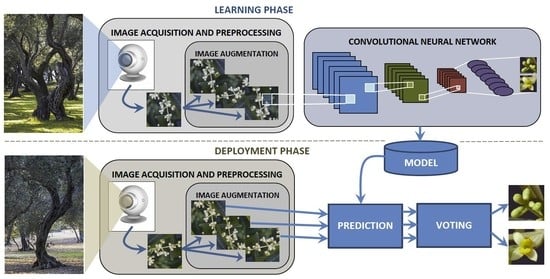
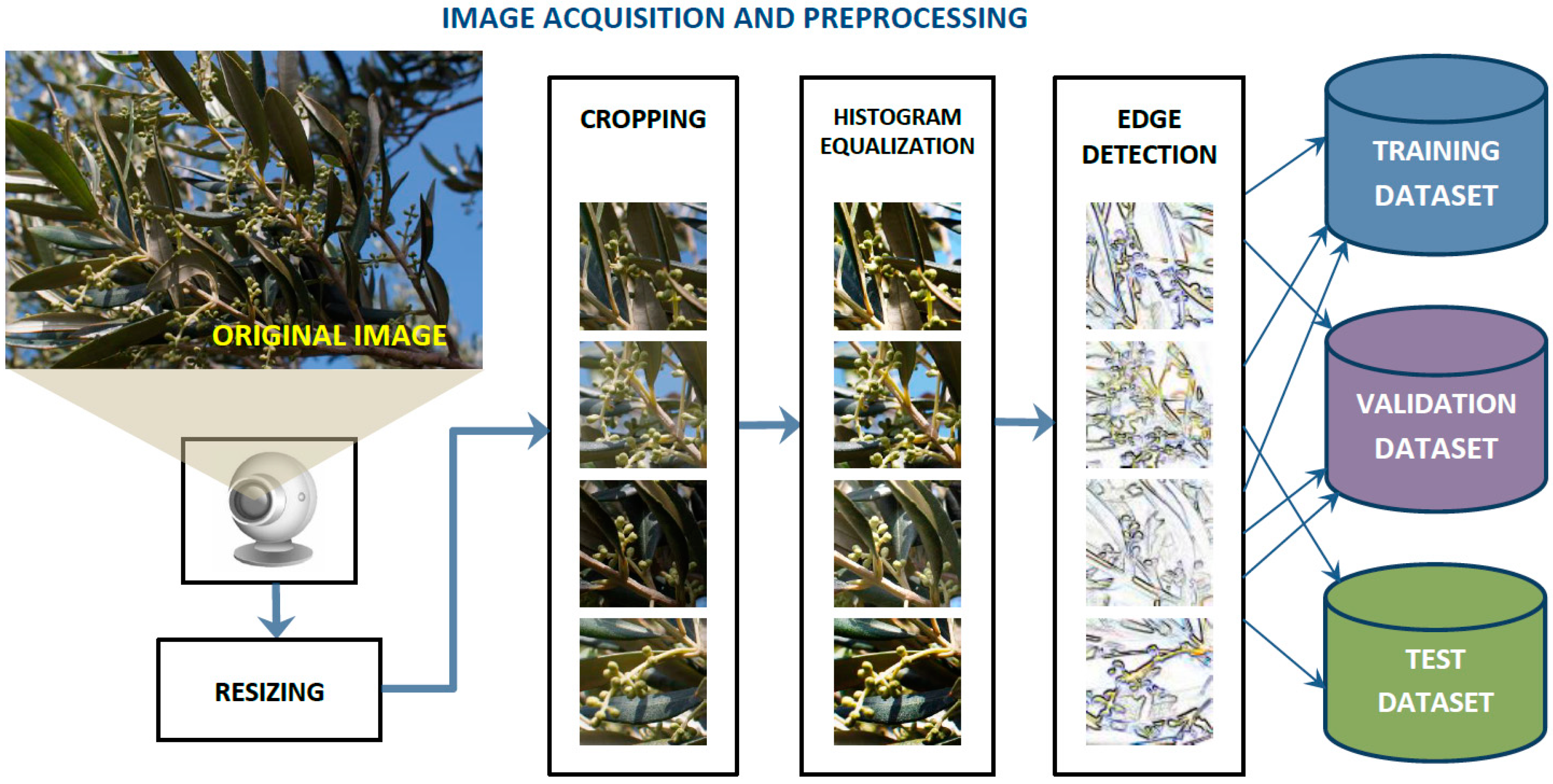
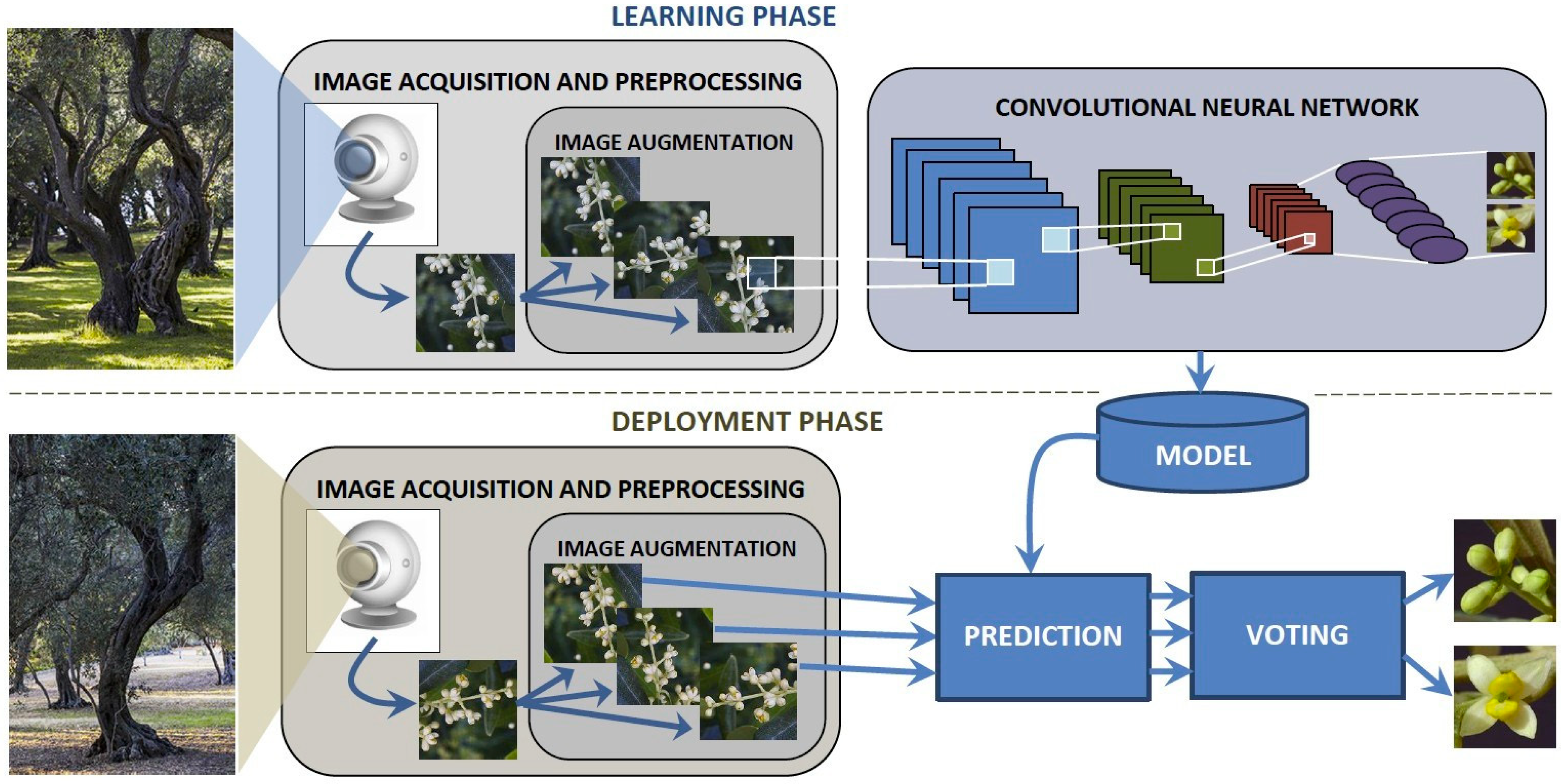
2. Materials and Methods
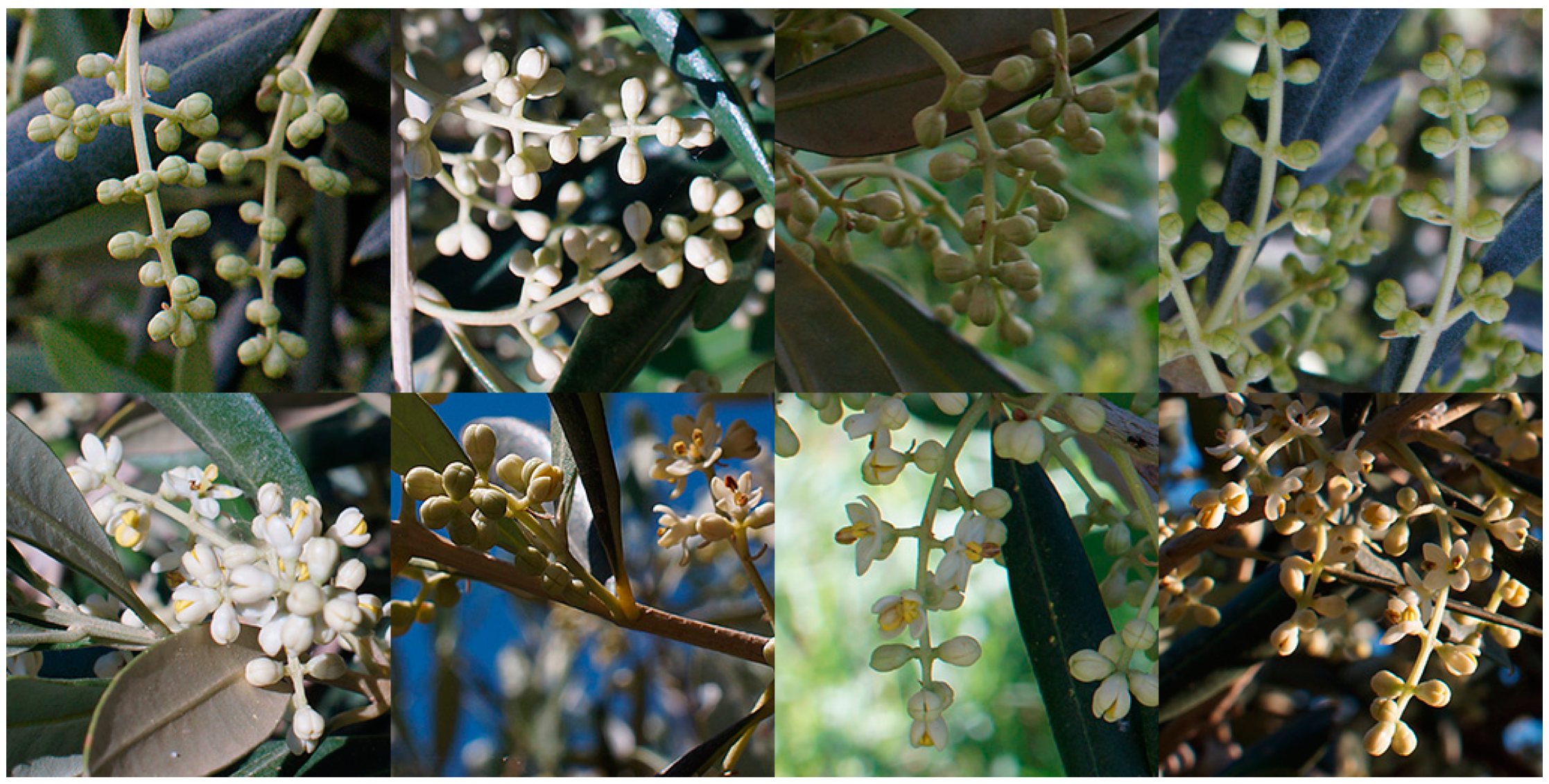
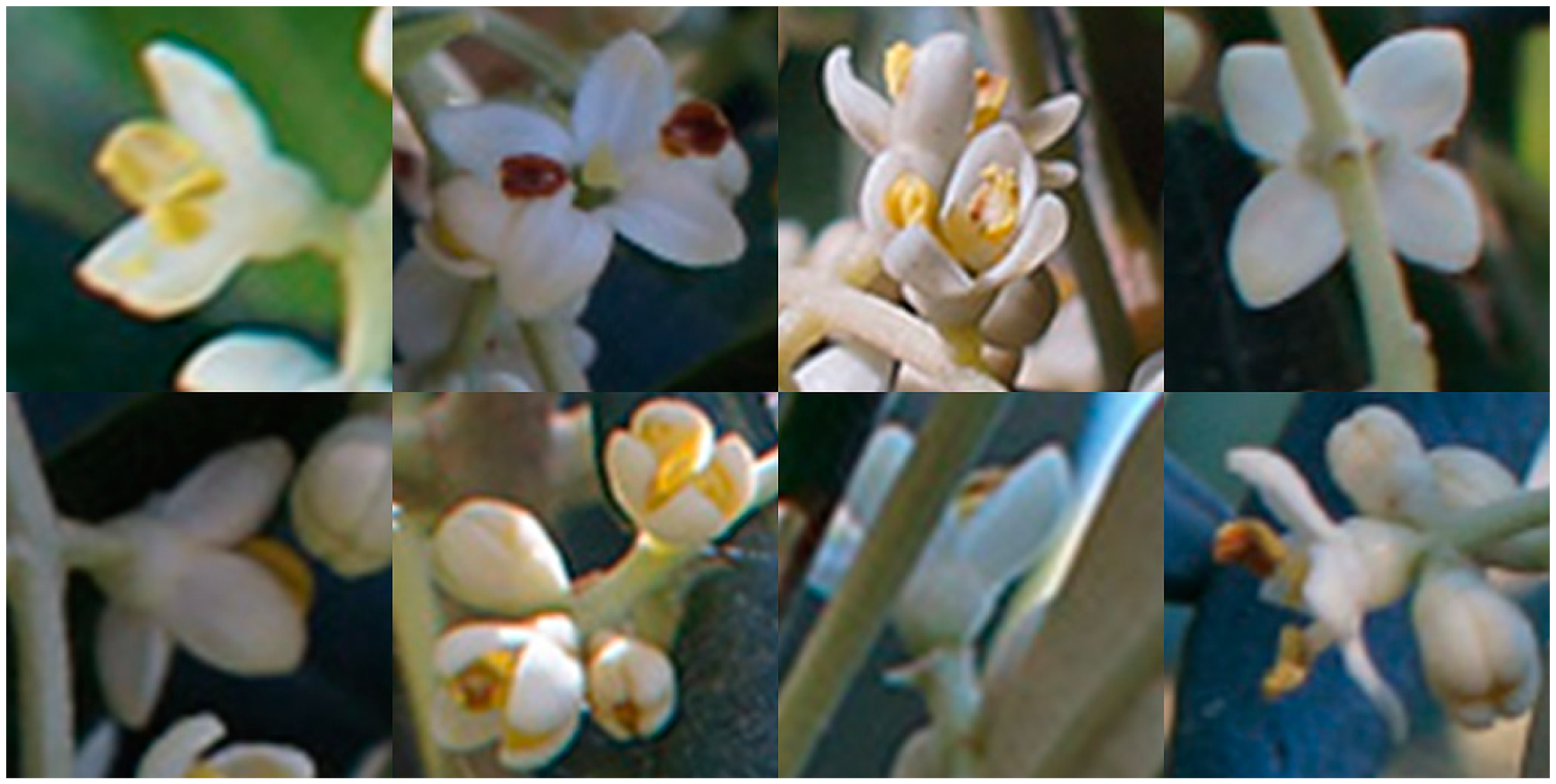
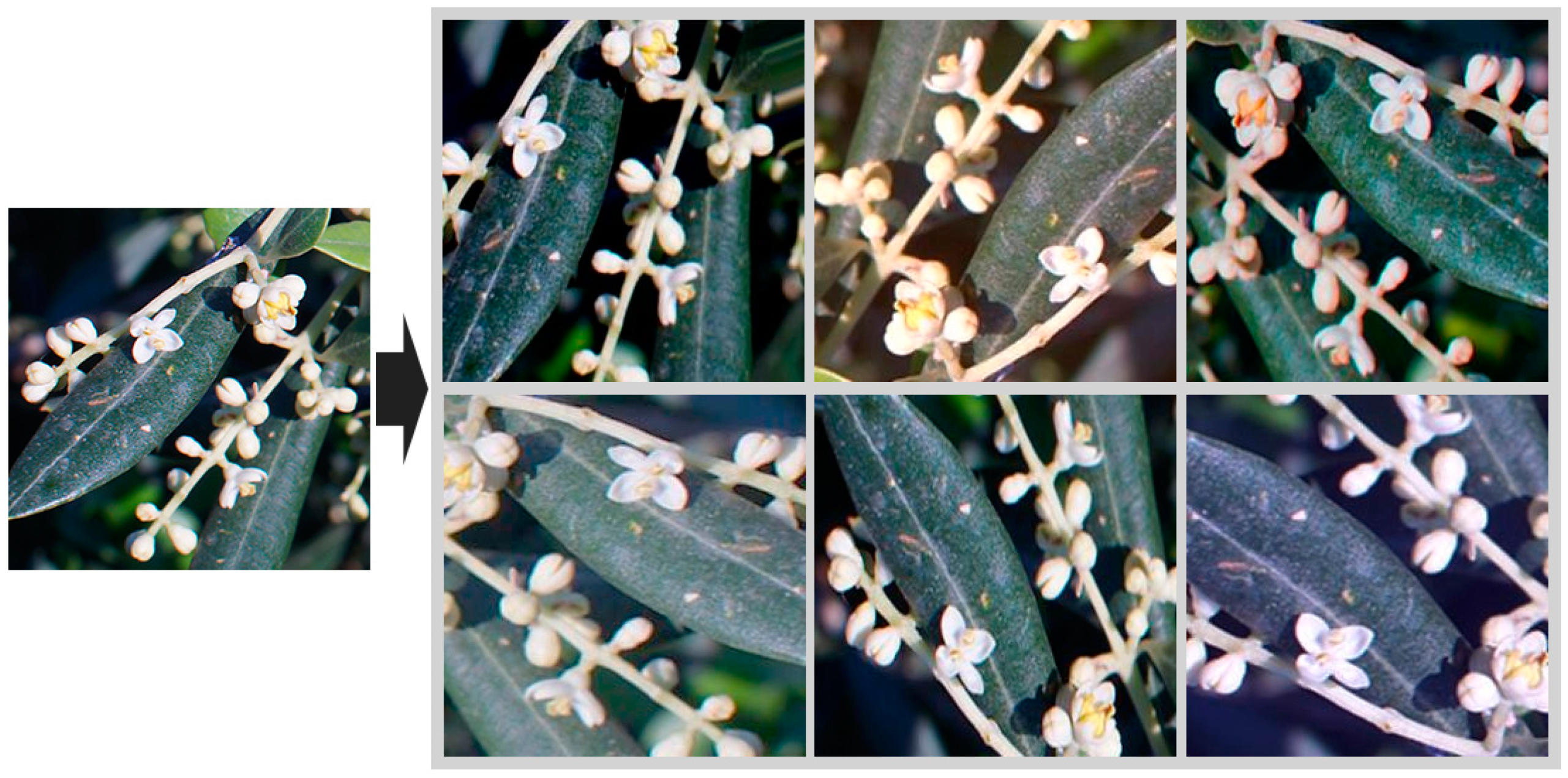
2.1. Dataset
2.2. Experimental Study
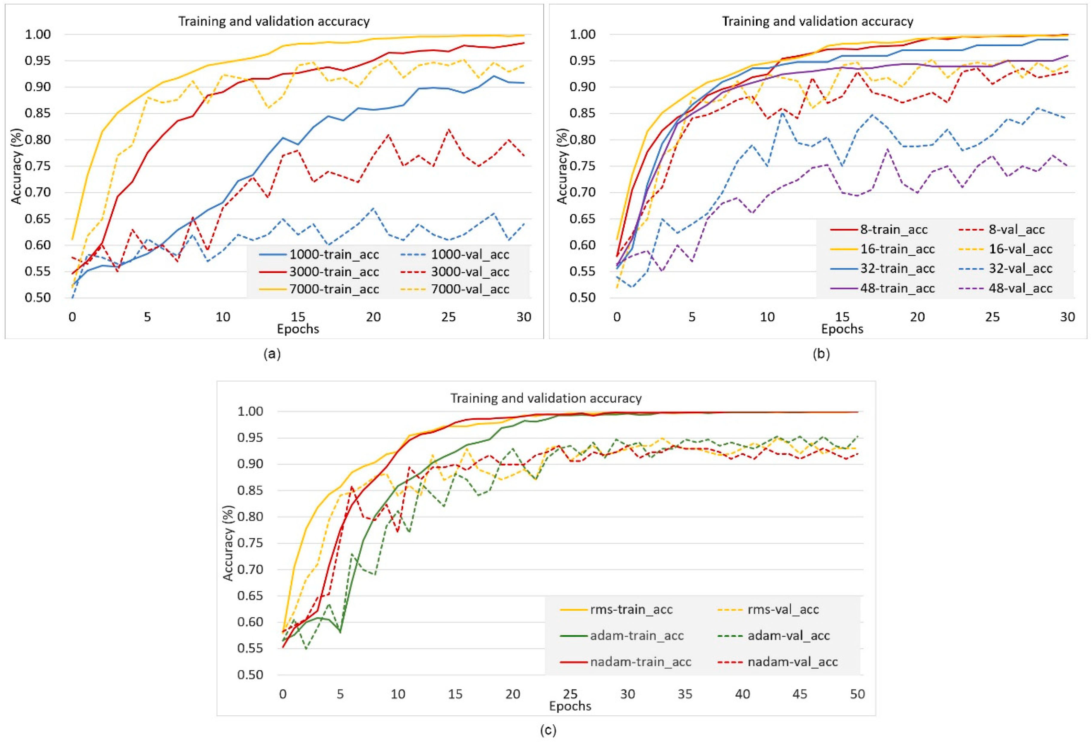
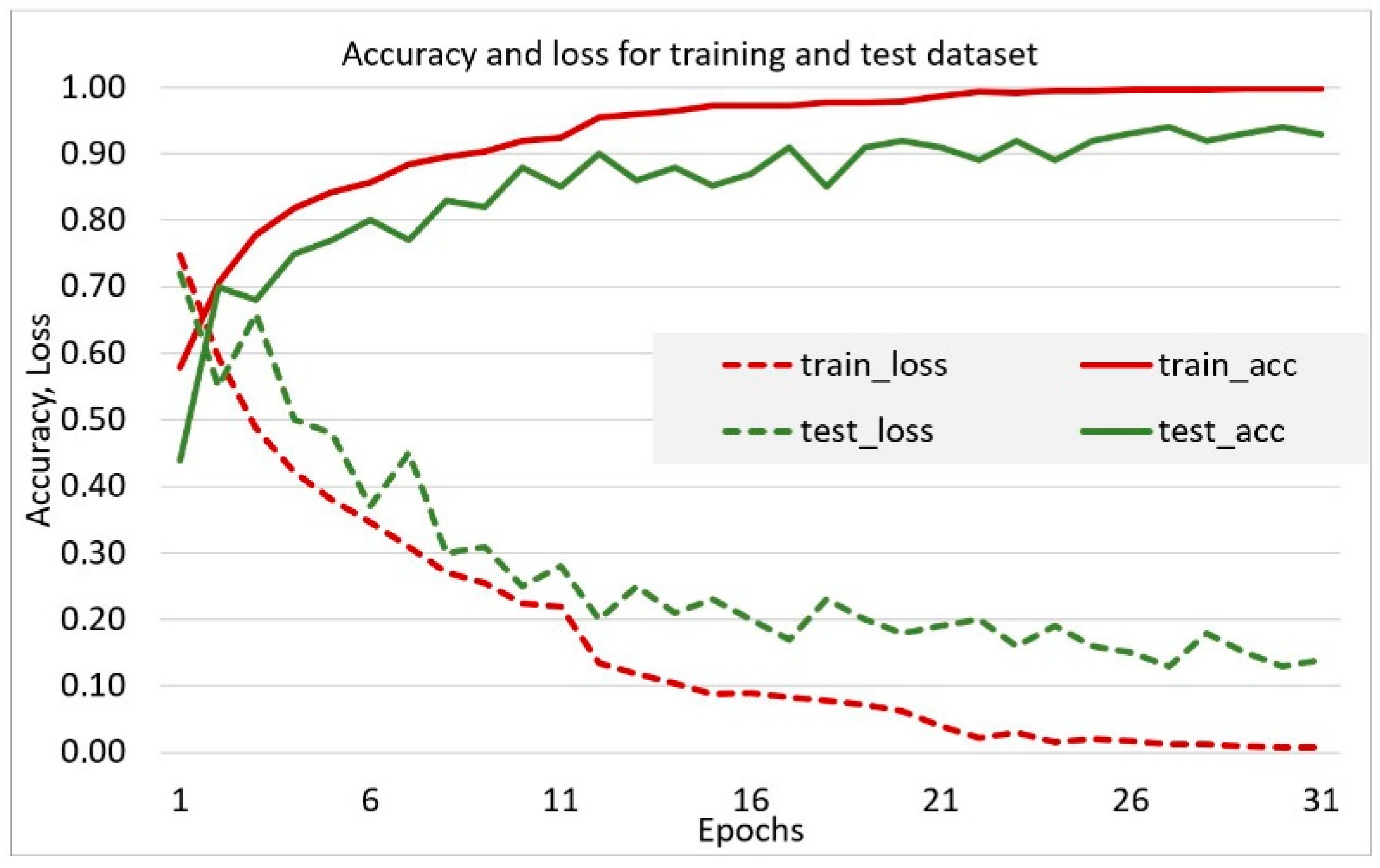
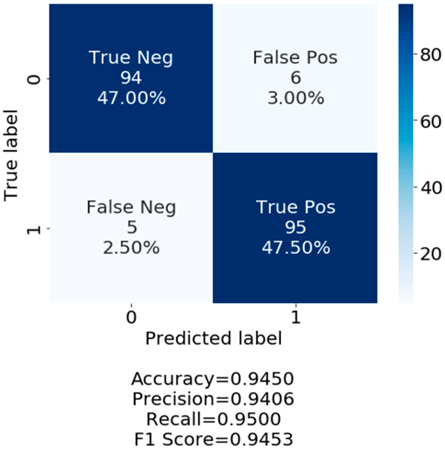
3. Results and Discussion
4. Conclusions
Author Contributions
Funding
Conflicts of Interest
References
- Moriondo, M.; Bindi, M. Impact of climate change on the phenology of typical Mediterranean crops. Ital. J. Agrometeorol. 2007, 3, 5–12. [Google Scholar]
- Gutierrez, A.P.; Ponti, L.; Cossu, Q.A. Effects of climate warming on olive and olive fly (Bactrocera oleae (Gmelin)) in California and Italy. Clim. Chang. 2009, 95, 195–217. [Google Scholar] [CrossRef]
- Tang, S.; Tang, G.; Cheke, R.A. Optimum timing for integrated pest management: Modelling rates of pesticide application and natural enemy releases. J. Theor. Biol. 2010, 264, 623–638. [Google Scholar] [CrossRef] [PubMed] [Green Version]
- Chuine, I.; Cour, P.; Rousseau, D.D. Selecting models to predict the timing of flowering of temperate trees: Implications for tree phenology modelling. Plant Cell Environ. 1999, 22, 1–13. [Google Scholar] [CrossRef] [Green Version]
- De Melo-Abreu, J.P.; Barranco, D.; Cordeiro, A.M.; Tous, J.; Rogado, B.M.; Villalobos, F.J. Modelling olive flowering date using chilling for dormancy release and thermal time. Agric. For. Meteorol. 2004, 125, 117–127. [Google Scholar] [CrossRef]
- Osborne, C.P.; Chuine, I.; Viner, D.; Woodward, F.I. Olive phenology as a sensitive indicator of future climatic warming in the Mediterranean. Plant Cell Environ. 2000, 23, 701–710. [Google Scholar] [CrossRef] [Green Version]
- Aguilera, F.; Fornaciari, M.; Ruiz-Valenzuela, L.; Galán, C.; Msallem, M.; Dhiab, A.B.; Díaz-de La Guardia, C.; del Mar Trigo, M.; Bonofiglio, T.; Orlandi, F. Phenological models to predict the main flowering phases of olive (Olea europaea L.) along a latitudinal and longitudinal gradient across the Mediterranean region. Int. J. Biometeorol. 2015, 59, 629–641. [Google Scholar] [CrossRef]
- Orlandi, F.; Vazquez, L.M.; Ruga, L.; Bonofiglio, T.; Fornaciari, M.; Garcia-Mozo, H.; Domínguez, E.; Romano, B.; Galan, C. Bioclimatic requirements for olive flowering in two Mediterranean regions located at the same latitude (Andalucia, Spain, and Sicily, Italy). Ann. Agric. Environ. Med. 2005, 12, 47. [Google Scholar]
- Garcia-Mozo, H.; Orlandi, F.; Galan, C.; Fornaciari, M.; Romano, B.; Ruiz, L.; de la Guardia, C.D.; Trigo, M.M.; Chuine, I. Olive flowering phenology variation between different cultivars in Spain and Italy: Modeling analysis. Theor. Appl. Climatol. 2009, 95, 385. [Google Scholar] [CrossRef]
- Oteros, J.; García-Mozo, H.; Vázquez, L.; Mestre, A.; Domínguez-Vilches, E.; Galán, C. Modelling olive phenological response to weather and topography. Agric. Ecosyst. Environ. 2013, 179, 62–68. [Google Scholar] [CrossRef]
- Herz, A.; Hassan, S.A.; Hegazi, E.; Nasr, F.N.; Youssef, A.A.; Khafagi, W.E.; Agamy, E.; Ksantini, M.; Jardak, T.; Mazomenos, B.E.; et al. Towards sustainable control of Lepidopterous pests in olive cultivation. Gesunde Pflanz. 2005, 57, 117–128. [Google Scholar] [CrossRef] [Green Version]
- Haniotakis, G.E. Olive pest control: Present status and prospects. IOBC/WPRS Bull. 2005, 28, 1. [Google Scholar]
- Hilal, A.; Ouguas, Y. Integrated control of olive pests in Morocco. IOBC/WPRS Bull. 2005, 28, 101. [Google Scholar]
- Kamilaris, A.; Prenafeta-Boldú, F.X. Deep learning in agriculture: A survey. Comput. Electron. Agric. 2018, 147, 70–90. [Google Scholar] [CrossRef] [Green Version]
- Raschka, S.; Mirjalili, V. Python Machine Learning: Machine Learning and Deep Learning with Python, Scikit-Learn, and TensorFlow 2; Packt Publishing Ltd.: Birmingham, UK, 2019. [Google Scholar]
- Perez, L.; Wang, J. The effectiveness of data augmentation in image classification using deep learning. arXiv preprint 2017, arXiv:1712.04621. Available online: https://arxiv.org/abs/1712.04621 (accessed on 11 October 2019).
- Meier, U.; Bleiholder, H.; Buhr, L.; Feller, C.; Hack, H.; Heß, M.; Lancashire, P.D.; Schnock, U.; Stauß, R.; Van Den Boom, T.; et al. The BBCH system to coding the phenological growth stages of plants–history and publications. J. Kult. 2009, 61, 41–52. [Google Scholar]
- Simonyan, K.; Zisserman, A. Very deep convolutional networks for large-scale image recognition. arXiv preprint 2014, arXiv:1409.1556. Available online: https://arxiv.org/abs/1409.1556 (accessed on 13 October 2019).
- Szegedy, C.; Ioffe, S.; Vanhoucke, V.; Alemi, A.A. Inception-v4, inception-resnet and the impact of residual connections on learning. In Proceedings of the Thirty-first AAAI Conference on Artificial Intelligence, San Francisco, CA, USA, 4–9 February 2017; pp. 4278–4284. [Google Scholar]
- Chollet, F. Xception: Deep learning with depthwise separable convolutions. In Proceedings of the IEEE Conference on Computer Vision and Pattern Recognition, Honolulu, HI, USA, 21–26 July 2017; pp. 1251–1258. [Google Scholar] [CrossRef] [Green Version]
- He, K.; Zhang, X.; Ren, S.; Sun, J. Deep residual learning for image recognition. In Proceedings of the IEEE Conference on Computer Vision and Pattern Recognition, Las Vegas, NV, USA, 27–30 June 2016; pp. 770–778. [Google Scholar] [CrossRef] [Green Version]
- Pan, S.J.; Yang, Q. A survey on transfer learning. IEEE Trans. Knowl. Data Eng. 2009, 22, 1345–1359. [Google Scholar] [CrossRef]
- Chollet, F. Deep Learning Mit Python und Keras: Das Praxis-Handbuch vom Entwickler der Keras-Bibliothek; MITP-Verlags GmbH & Co. KG.: Bonn, Germany, 2018. [Google Scholar]
- Abadi, M.; Agarwal, A.; Barham, P.; Brevdo, E.; Chen, Z.; Citro, C.; Corrado, G.S.; Davis, A.; Dean, J.; Devin, M.; et al. Tensorflow: Large-scale machine learning on heterogeneous distributed systems. arXiv preprint 2016, arXiv:1603.04467. Available online: https://arxiv.org/abs/1603.04467 (accessed on 20 October 2019).
- Maas, A.L.; Hannun, A.Y.; Ng, A.Y. Rectifier nonlinearities improve neural network acoustic models. In Proceedings of the ICML, Atlanta, GA, USA, 16–31 June 2013; Volume 30, p. 3. [Google Scholar]
- Tieleman, T.; Hinton, G. Lecture 6.5-rmsprop: Divide the gradient by a running average of its recent magnitude. COURSERA Neural Netw. Mach. Learn. 2012, 4, 26–31. [Google Scholar]
- Ioffe, S.; Szegedy, C. Batch normalization: Accelerating deep network training by reducing internal covariate shift. arXiv preprint 2015, arXiv:1502.03167. Available online: https://arxiv.org/abs/1502.03167 (accessed on 10 October 2019).
- Srivastava, N.; Hinton, G.; Krizhevsky, A.; Sutskever, I.; Salakhutdinov, R. Dropout: A simple way to prevent neural networks from overfitting. J. Mach. Learn. Res. 2014, 15, 1929–1958. [Google Scholar]
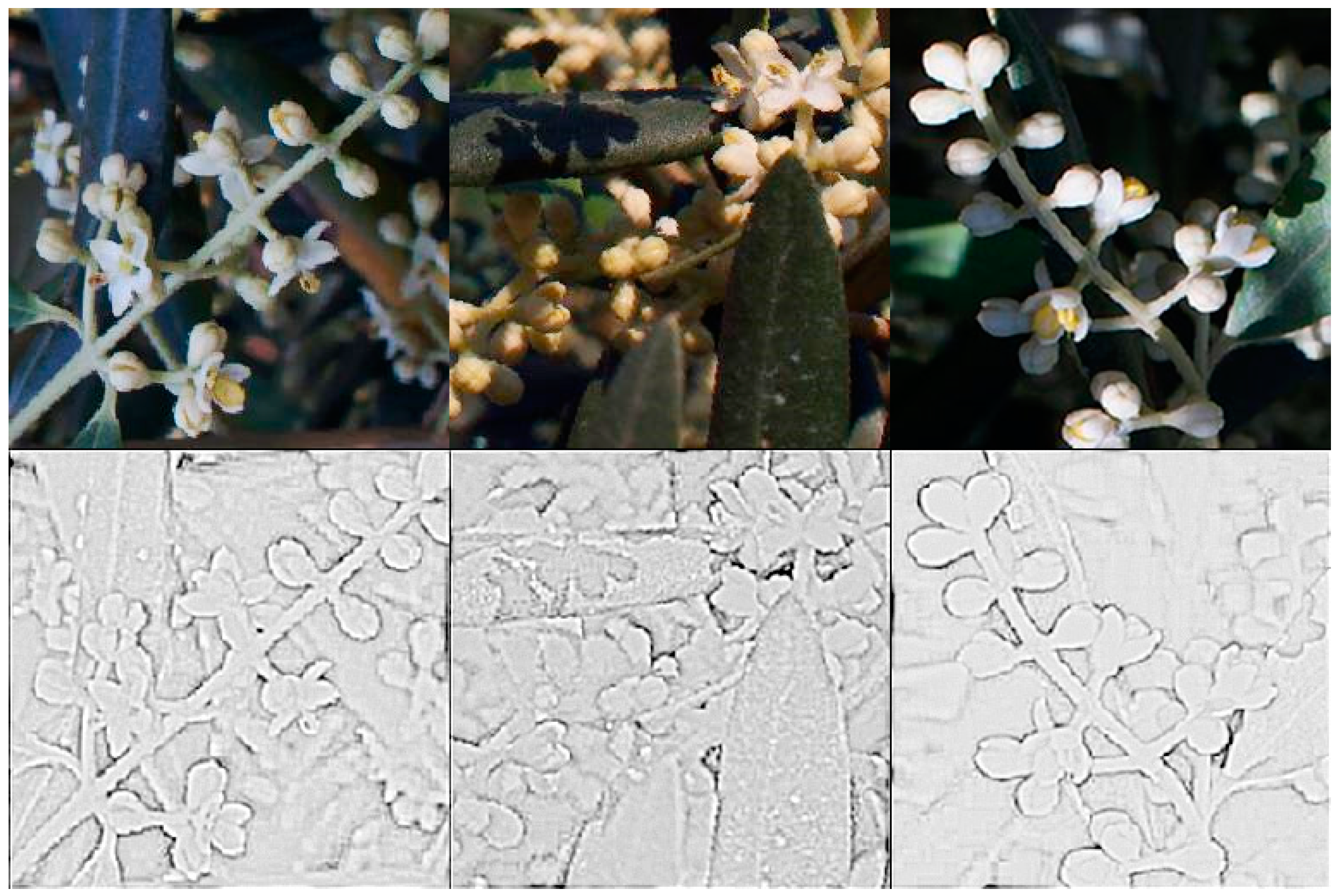
- Asghari, M.H.; Jalali, B. Edge detection in digital images using dispersive phase stretch transform. Int. J. Biomed. Imaging 2015. [Google Scholar] [CrossRef] [Green Version]
- Jalali, B.; Suthar, M.; Asghari, M.; Mahjoubfar, A. Time Stretch Inspired Computational Imaging. arXiv preprint 2017, arXiv:1706.07841. Available online: https://arxiv.org/abs/1706.07841 (accessed on 20 September 2019).
- Ang, R.B.Q.; Nisar, H.; Khan, M.B.; Tsai, C.Y. Image segmentation of activated sludge phase contrast images using phase stretch transform. Microscopy 2019, 68, 144–158. [Google Scholar] [CrossRef] [PubMed]
- Masters, D.; Luschi, C. Revisiting small batch training for deep neural networks. arXiv preprint 2018, arXiv:1804.07612. Available online: https://arxiv.org/abs/1804.07612 (accessed on 20 October 2019).
- Kingma, D.P.; Ba, J. Adam: A method for stochastic optimization. arXiv preprint 2014, arXiv:1412.6980. Available online: https://arxiv.org/abs/1412.6980 (accessed on 10 October 2019).
- Dozat, T. Incorporating Nesterov Momentum into Adam. In Proceedings of the 4th International Conference on Learning Representations, Workshop Track, San Juan, Puerto Rico, 2–4 May 2016. [Google Scholar]
- Rojo, J.; Pérez-Badia, R. Models for forecasting the flowering of Cornicabra olive groves. Int. J. Biometeorol. 2015, 59, 1547–1556. [Google Scholar] [CrossRef]
- Mancuso, S.; Pasquali, G.; Fiorino, P. Phenology modelling and forecasting in olive (Olea europaea L.) using artificial neural networks. Adv. Hortic. Sci. 2002, 16, 155–164. [Google Scholar]
- Barzman, M.; Bàrberi, P.; Birch, A.N.E.; Boonekamp, P.; Dachbrodt-Saaydeh, S.; Graf, B.; Hommel, B.; Jensen, J.E.; Kiss, J.; Kudsk, P.; et al. Eight principles of integrated pest management. Agron. Sustain. Dev. 2015, 35, 1199–1215. [Google Scholar] [CrossRef]


| CNN | Depth | Dataset | Parameters | Accuracy (%) |
|---|---|---|---|---|
| VGG19 | 19 | Augm. | 24,219,106 | 69.50 |
| VGG19 (pretrained) | 19 | Augm. | 24,219,106 | *54.00 |
| InceptionResNetV2 | 164 | Augm. | 55,912,674 | 65.50 |
| InceptionResNetV2 (pretrained) | 164 | Augm. | 55,912,674 | 66.50 |
| Xception (pretrained) | 71 | Augm. | 22,910,480 | 67.00 |
| ResNet50 | 50 | Augm. | 25,687,938 | 64.00 |
| ResNet50 (pretrained) | 50 | Augm. | 25,687,938 | *54.00 |
| Custom CNN | 12 | Augm. | 3,614,768 | 91.50 |
| Custom CNN | 13 | Augm. | 3,746,402 | 93.50 |
| Custom CNN | 14 | Orig. | 6,106,242 | 88.50 |
| Custom CNN | 14 | Augm. | 6,106,242 | 94.50 |
| Custom CNN | 15 | Augm. | 6,892,130 | 93.50 |
| Custom CNN | 16 | Augm. | 10,039,458 | 91.50 |
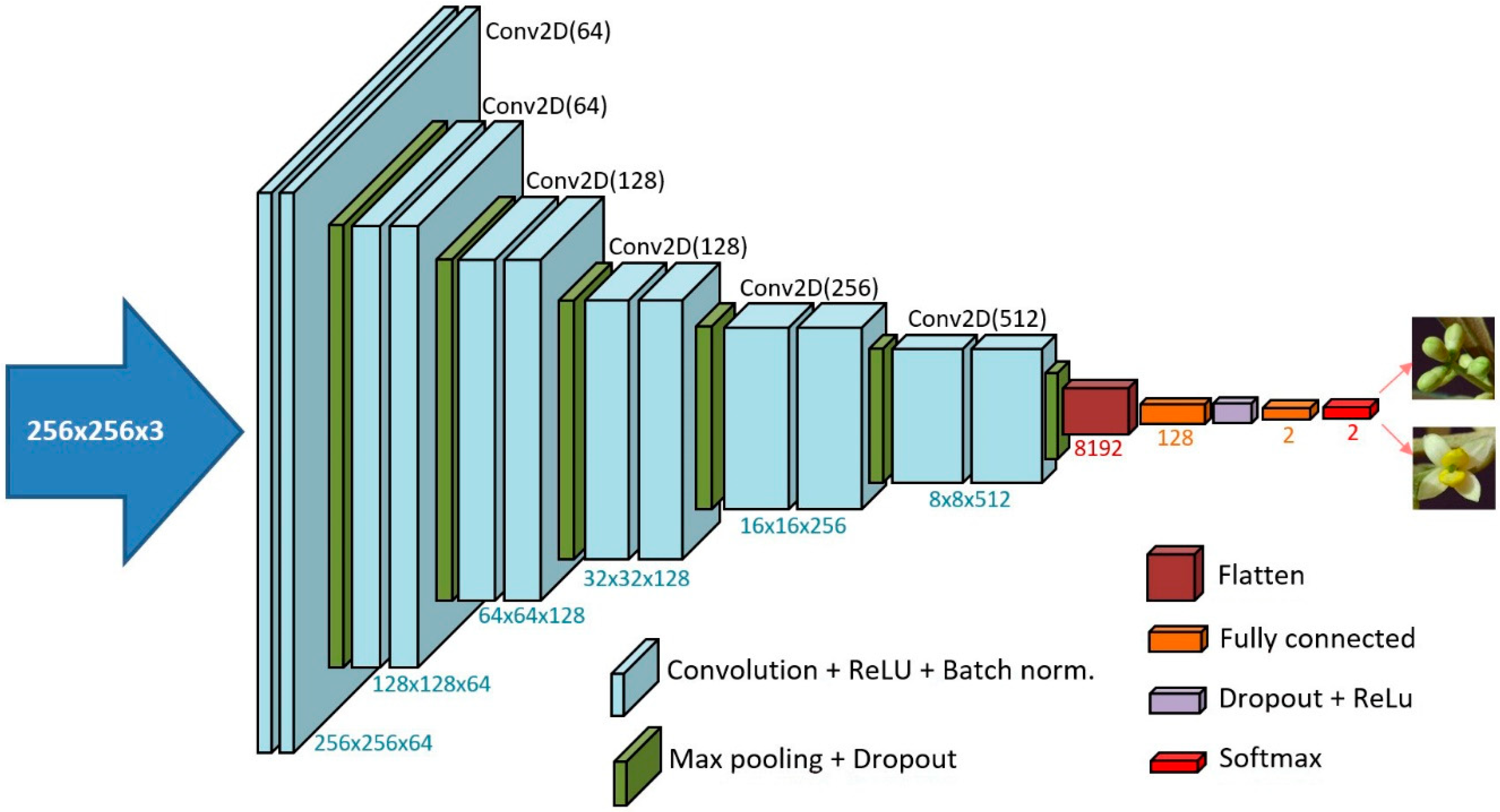
| Layer Type | Output Shape | #Param |
|---|---|---|
| Input | 256 × 256×3 | - |
| Conv2D(64) | 256 × 256 × 64 | 640 |
| ACT(LReLu)-BN | 256 × 256 × 64 | 1,024 |
| Conv2D(64) | 256 × 256 × 64 | 36,928 |
| ACT(LReLu)-BN | 256 × 256 × 64 | 1,024 |
| MP(2,2)+DR(0.1) | 128 × 128 × 64 | - |
| Conv2D(64) | 128 × 128 × 64 | 36,928 |
| ACT(LReLu)-BN | 128 × 128 × 64 | 512 |
| Conv2D(64) | 128 × 128 × 64 | 36,928 |
| ACT(LReLu)-BN | 128 × 128 × 64 | 512 |
| MP(2,2)+DR(0.2) | 64 × 64 × 64 | - |
| Conv2D(128) | 64 × 64 × 128 | 73,856 |
| ACT(LReLu)-BN | 64 × 64 × 128 | 256 |
| Conv2D(128) | 64 × 64 × 128 | 147,584 |
| ACT(LReLu)-BN | 64 × 64 × 128 | 256 |
| MP(2,2)+DR(0.1) | 32 × 32 × 128 | - |
| Conv2D(128) | 32 × 32 × 128 | 147,584 |
| ACT(LReLu)-BN | 32 × 32 × 128 | 128 |
| Conv2D(128) | 32 × 32 × 128 | 147,584 |
| ACT(LReLu)-BN | 32 × 32 × 128 | 128 |
| MP(2,2)+DR(0.2) | 16 × 16 × 128 | - |
| Conv2D(256) | 16 × 16 × 256 | 295,168 |
| ACT(LReLu)-BN | 16 × 16 × 256 | 64 |
| Conv2D(256) | 16 × 16 × 256 | 590,080 |
| ACT(LReLu)-BN | 16 × 16 × 256 | 64 |
| MP(2,2)+DR(0.2) | 8 × 8 × 256 | - |
| Conv2D(256) | 8 × 8 × 512 | 1,180,160 |
| ACT(LReLu)-BN | 8 × 8 × 512 | 32 |
| Conv2D(256) | 8 × 8 × 512 | 2,359,808 |
| ACT(LReLu)-BN | 8 × 8 × 512 | 32 |
| MP(2,2)+DR(0.2) | 4 × 4 × 512 | - |
| Flatten | 8192 | - |
| Dense(128) | 128 | 1,048,704 |
| ACT(LReLu)-DR(0.3) | 128 | - |
| Dense(2) | 2 | 258 |
| ACT(softmax) | 2 | - |
| TOTAL | 6,106,242 |
© 2020 by the authors. Licensee MDPI, Basel, Switzerland. This article is an open access article distributed under the terms and conditions of the Creative Commons Attribution (CC BY) license (http://creativecommons.org/licenses/by/4.0/).
Share and Cite
Milicevic, M.; Zubrinic, K.; Grbavac, I.; Obradovic, I. Application of Deep Learning Architectures for Accurate Detection of Olive Tree Flowering Phenophase. Remote Sens. 2020, 12, 2120. https://doi.org/10.3390/rs12132120
Milicevic M, Zubrinic K, Grbavac I, Obradovic I. Application of Deep Learning Architectures for Accurate Detection of Olive Tree Flowering Phenophase. Remote Sensing. 2020; 12(13):2120. https://doi.org/10.3390/rs12132120
Chicago/Turabian StyleMilicevic, Mario, Krunoslav Zubrinic, Ivan Grbavac, and Ines Obradovic. 2020. "Application of Deep Learning Architectures for Accurate Detection of Olive Tree Flowering Phenophase" Remote Sensing 12, no. 13: 2120. https://doi.org/10.3390/rs12132120