Classification of Oil Slicks and Look-Alike Slicks: A Linear Discriminant Analysis of Microwave, Infrared, and Optical Satellite Measurements

Abstract

We classify low-backscatter regions observed in Synthetic Aperture Radar (SAR) measurements of the surface of the ocean as either oil slicks or look-alike slicks (radar false targets). Our proposed classification algorithm is based on Linear Discriminant Analyses (LDAs) of RADARSAT-1 measurements (402 scenes off the southeast coast of Brazil from July 2001 to June 2003) and Meteorological-Oceanographic (MetOc) data from other earth observation sensors: Advanced Very High Resolution Radiometer (AVHRR), Sea-Viewing Wide Field-of-View Sensor (SeaWiFS), Moderate Resolution Imaging Spectroradiometer (MODIS), and Quick Scatterometer (QuikSCAT). Oil slicks are sea-surface expressions of exploration and production oil, ship- and orphan-spills. False targets are associated with environmental phenomena, such as biogenic films, algal blooms, upwelling, low wind, or rain cells. Both categories have been interpreted by domain-experts: mineral oil (n = 350; 45.5%) and petroleum free (n = 419; 54.5%). We explore nine size variables (area, perimeter, etc.) and three types of MetOc information (sea surface temperature, chlorophyll-a, and wind speed) that describe the 769 samples analyzed. Seven attribute–domain combinations are tested with three non-linear transformations (none, cube root, log₁₀), with and without MetOc, adding to 39 attribute subdivisions. Classification accuracies are independent of data transformation and improve when selected size attributes are combined with MetOc, leading to overall accuracies of ~80% and sound levels of sensitivity (~90%), specificity (~80%), positive (~80%) and negative (~90%) predictive values. The effectiveness of this data-driven attempt supports further commercial or academic implementation of our LDA algorithm.

1. Introduction

The presence and development of oil and gas exploration and production in open oceanic waters of Brazil has led to many environmental oil-related incidents over time, and two major episodes have occurred since the eve of the current millennium. In 2001, the world’s largest floating offshore oilrig at the time (P-36) sank in Brazilian waters, and the many tonnes of crude oil it had on board were spilled into the sea [1]. This is still considered one of the most terrible international petroleum industry disasters [2]. More recently, in 2019, a unique and worldwide-reported massive oil spill polluted hundreds of kilometers of coastal ecosystems in Brazil over the course of many months (from August until December), deemed Brazil’s worst environmental petroleum-related tragedy [3,4]—the circumstances of the initial source and when it was released still unknown [5,6].

Satellites can be used to assist in locating oil contamination and potential candidate sources on the sea surface. However, ambiguous interpretations of satellite data can be dismissed as false warnings [7]. The importance of timely and strategic environmental response efforts highlights the need for improved remote sensing surveillance methods capable of correctly identifying petroleum pollution on the surface of the ocean. Thus, improved remote sensing methods of differentiating mineral oil slicks (sea-surface footprint of natural oil seeps or anthropogenic oil spills) from other possible petroleum-free false targets (often referred to as “slick look-alikes” or “slick-alikes”) are a constant and pressing need for effectively guiding countermeasures to combat oil pollution in our oceans.

Different types of satellite-borne sensors are used to study oil slicks [8] such as Synthetic Aperture Radars (SAR; [9]), Advanced Very High Resolution Radiometer (AVHRR; [10]), Sea-Viewing Wide Field-of-View Sensor (SeaWiFS; [11]), Moderate Resolution Imaging Spectroradiometer (MODIS; [12]), etc. Arguably, the best suited is SAR, but it is prone to false alarms as the oil signature is not unique [13]. As with slicks from mineral oil, look-alike slicks are also detected in SAR imagery as low-backscatter regions, caused by the slicks dampening the roughness of the ocean surface, i.e., smooth texture regions [14]. Radar false targets are frequently observed and correspond to other environmental phenomena such as biogenic films, algal blooms, upwelling, low wind, rain cells, internal gravitational waves, and others [15].

Three main processes play important roles in the investigation of oil slicks with SAR:

• Separation of smooth (low radar signal) and rough (sea clutter) texture regions, e.g., [16];
• Discrimination between oil slicks and slick look-alikes, e.g., [17]; and
• Differentiation between oil seeps and oil spills, e.g., [18].

The first process proposes polygons with oil slicks or petroleum-free candidates (e.g., [19]), and the other two build on that. While some scientific effort has been put in to investigating non-linear techniques for discriminating polygons containing oil and those that do not (e.g., [20]), only recently have Linear Discriminant Analyses (LDAs) been employed to automatically distinguish seeps from spills (e.g., [21,22,23,24]).

Based on the seep-spill discrimination findings of [18], in this paper, we extend the methodological recommendations of [21,22,23,24] with the objective to classify regions where sea-surface backscatter in SAR measurements are low as either mineral oil slicks or other environmental petroleum-free false targets (i.e., oil vs. look-alikes). For this, we use an algorithm that exploits LDAs of a set of satellite measurements (microwave, infrared, and optical) off the southeast coast of Brazil (Figure 1). Through the scientific settings of our study we use an existing database to seek the answers of six questions:

• Is a simple, linear, multivariate data analysis technique able to discriminate between oil slicks and petroleum-free slicks?
• Is it feasible to reach classification accuracy levels to support operational implementations (commercial or academic) of our proposed algorithm?
• Does the application of non-linear data transformations affect the oil and look-alike discrimination?
• Can the sole use of Meteorological-Oceanographic (MetOc) satellite information distinguish oil from false targets?
• Is there any specific combination of attributes that leads to a superior discrimination between oil slicks and slick-alikes?
• Is our LDA-developed algorithm applicable to other regions?

1.1. Linear Differentiation Background: Seeps vs. Spills

1.1.1. Human-Dependent Operational Guidelines

The ability to discriminate between seeps and spills using the synoptic view of satellites has long been an objective at the Laboratory of Radar Remote Sensing Applied to the Petroleum Industry (LabSAR) of the Federal University of Rio de Janeiro (UFRJ, Brazil). For about two decades, LabSAR has provided a valuable tool to oil and gas operators: the most probable location of offshore petroleum systems based on satellite imagery analyses—e.g., [25]. However, these were operational projects that relied on manual approaches, i.e., dependent on human intervention. The paradigm against the widely-used manual seep-spill image inspection processes versus newly-developed automatic methods has been the focus of recent academic studies—e.g., [18]. Within this scope, a fresh take on an old, well-established problem has indeed shown its facet as described below.

1.1.2. Initial Automated Procedure: Carvalho

In this section we summarize past research and results of [18] who developed an automated procedure to classify sea-surface expressions of mineral oil slicks into naturally seeped oil or operational oil spills with a linear multivariate analysis technique applied to SAR measurements, i.e., LDAs applied to RADARSAT-2 measurements from the Gulf of Mexico (Campeche Bay, Mexico). While [26,27] described the Mexican dataset used in [18], the bases of the exploratory analysis of [18] are discussed in depth in [21]. A single non-linear transformation was tested and applied to the data: log₁₀. Two distinct methods were used to select the most relevant variables—Correlation-Based Feature Selection (CFS; [28]) and Unweighted Pair Group Method with Arithmetic Mean dendrograms (UPGMA; [29]). The latter uses two user-defined thresholds: Pearson’s r correlation coefficients of 0.5 and ~0.9 [18,21]. The best overall seep-spill discrimination accuracy was about 70% with sensitivity (~80%), specificity (~75%), positive (~65%) and negative (~75%) predictive values. However, a linear transformation (Principal Component Analysis; PCA) was used to reduce the dimensionality of their selected variables, and as such, the “scores” of the relevant axes (i.e., principal components; PCs) were input into their LDAs. Additionally, by exploiting the entire attribute set, including particular contextual site-specific variables (e.g., latitude and longitude), they reached an almost faultless differentiation of 99.98%. Conversely, it was not possible to discriminate seeps from spills when the SAR-signature attributes were calculated with uncalibrated Digital Number (DN) values.

In this paper, we refer to the work of [18] and [21] simply as “Carvalho”. To summarize, Carvalho has demonstrated two particularly relevant issues:

• The feasibility of automatically separating oil (seeps) from oil (spills) using a simple, classical, linear classification method—i.e., LDA; and
• The possibility of achieving an effective seep-spill discrimination exploiting two straightforwardly calculated oil slick basic morphological characteristics (area and perimeter; after using a PCA), calculated from satellite measurements.

1.1.3. Subsequent Investigations: Carvalho et al.

In subsequent investigation, [22,23] promoted a refinement of Carvalho’s research in a more controlled manner. They applied eight non-linear transformations to the data: none (x), reciprocal (1/x), logarithm base 10 (log₁₀(x)), Napierian logarithm (ln(x)), square root (x^1/2), square power (x²), cube root (x^1/3), and cube power (x³). Four methods were tested for selecting uncorrelated attributes based on the UPGMA, which were preferable to the automated CFS due to its user-defined capabilities: 1) no UPGMA without PCA (i.e., original correlated data); 2) no UPGMA with PCA; 3) UPGMA without PCA; and 4) UPGMA with PCA (as in Carvalho). The UPGMA in these cases used a stricter threshold (0.3 > r > −0.3) deeming variables to be uncorrelated at this level based on the number of samples [30]. The best discrimination accuracies occurred with attribute selection method #1 (but this is not valid as it uses correlated variables), then #2 (PCA directly from the original data), closely followed by #3 (UPGMA alone), with #4 (UPGMA+PCA) being the least accurate. These results showed that the sole use of dendrograms (with the strict threshold, thus eliminating the application of PCAs, as proposed by Carvalho) is sufficient to effectively discriminate seeps from spills. The best data transformations to discriminate the oil slick category are log₁₀ and cube root, both producing classification accuracies similar to Carvalho.

Follow-up research by [24] also investigated ways to improve the LDA seep-spill classification. Variables were selected with the strict UPGMA threshold used in [22,23]. The two best non-linear transformations were compared with the original data. They showed that with no transformation applied, the discrimination was void. On the other hand, when the data were non-linearly transformed, the ability to discriminate was comparable to Carvalho, with log₁₀ being somewhat superior to cube root.

Together, the work reported by [22,23] and [24] is hereafter referred to as “Carvalho et al.”. Their major contributions are as follows:

• The superiority of non-linear data transformations: log₁₀ and cube root;
• The use of strict UPGMA (0.3 > r > −0.3) for selecting uncorrelated variables; and
• The optimal discrimination performance of the actual values of a few size variables ratios: perimeter-to-area (PtoA) and compact index (CMP=(4.π.area)/(perimeter²))—both in the log₁₀ transformed sets, thus far accompanied by fractal index (FRA=(2.ln(perimeter/4))/(ln(area))) in the cube cases.

1.1.4. Comparing Gulf of Mexico and Campos Basin Studies

The foremost characteristics of the LDA usage that can be highlighted between these previous works and our current paper are:

• Targets: Oil seeps and oil spills were classified, whereas here oil slicks are differentiated from slick-alikes;
• Location: The Mexican coast in the Gulf of Mexico was the initial study area, and here signals off the coast of Brazil are investigated—see Section 2.1;
• Data: While more than 4500 targets were used in the earlier studies, only about 750 samples are available for the current analysis; both studies have similarly balanced dichotomy distributions of ~50% per category—see Section 2.2;
• Satellites: RADARSAT-2 (VV-polarized, 16-bit) was used in the Gulf of Mexico studies, whereas here RADARSAT-1 (HH-polarized, 8-bit) data are used—see Section 2.2.1;
• Variables: In the previous studies, a wide-range of descriptors was used: SAR-signatures in gamma-, beta-, and sigma-naught (backscatter coefficients) measured in amplitude and decibels with and without a despeckle filter, augmented by size variables. Here, SAR-signature coefficients are not used, but we incorporate size and MetOc-information—see Section 3.1;
• Attribute Combinations: While Carvalho tested 44 attribute subdivisions [18,21], and Carvalho et al. explored many combinations: 32 in [22,23] and 61 in [24], here, 39 new attribute subdivisions were used—see Section 3.2;
• Objectives: Both studies, i.e., theirs and ours, are directed at developing algorithms to automate what is done by trained domain experts interpreting satellite imagery to routinely tell apart two types of target-slicks observed on the sea surface.

To further address the issues revealed in the automated LDA seep-spill discrimination, in this current paper we focus on investigating the application of such classical, linear, multivariate data analysis technique to tell apart oil slicks and look-alikes. The evolution of the concepts considered here is given below.

2. Materials and Methods

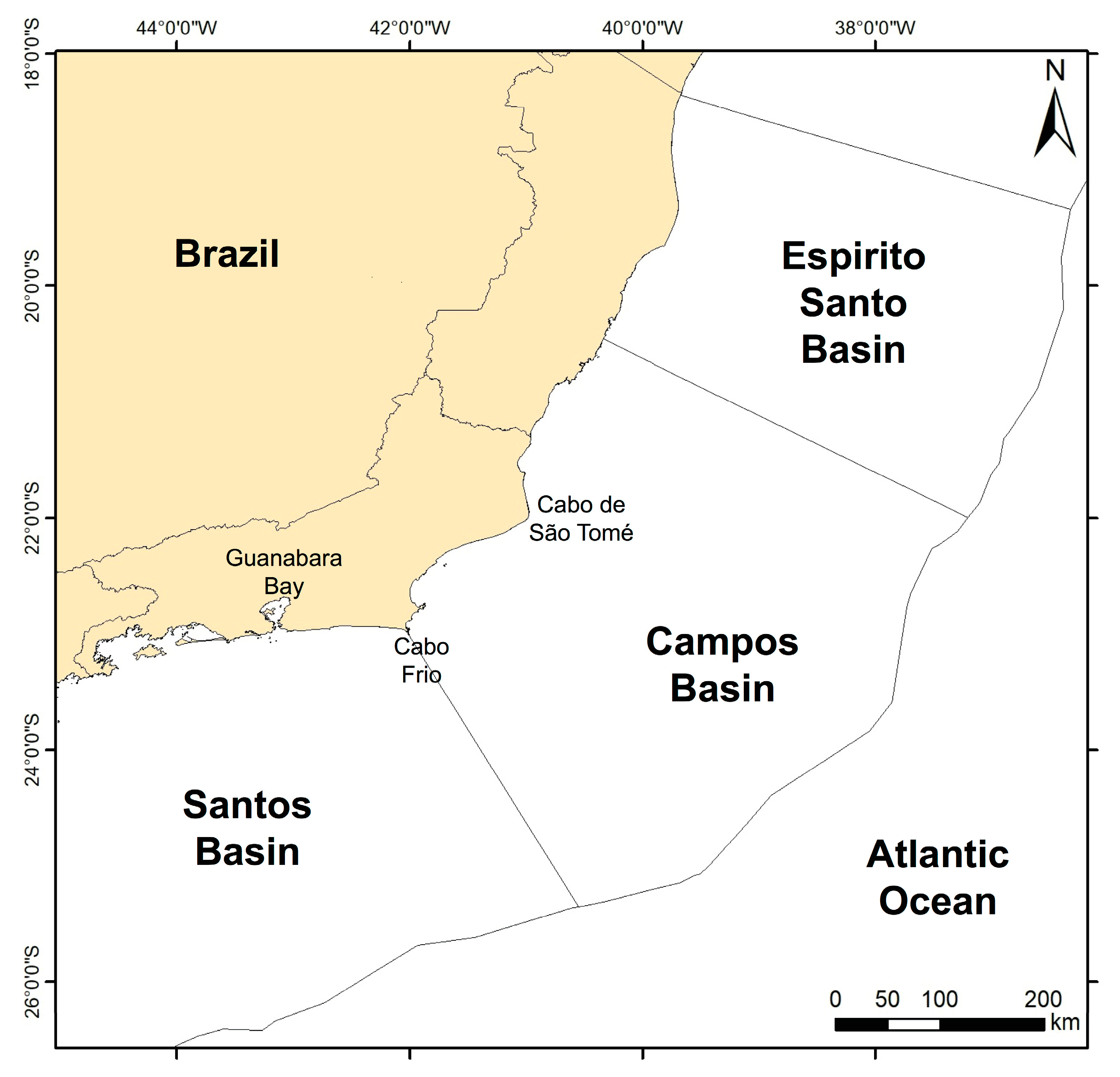
2.1. Study Area

The slicks investigated here (oil and look-alikes) are from a region off the southeast coast of Brazil: the Campos Basin (Figure 1). A large number of oil and gas exploration and production facilities are located in this basin, making it a province of significant politico-economic and socio-ecological relevance [31]. Since the mid-2000s, with the discovery of supergiant reservoirs of light hydrocarbons beneath the salt layers, the Campos Basin major petroleum-related infrastructure has been improved, and its worldwide economical relevance also increased; currently, 38 operational oilfields are responsible for providing 41.5% of Brazil’s oil and natural gas production: 1,373,068 barrels of equivalent oil per day [32].

The Campos Basin has a very dynamic environment that is subject to highly variable weather conditions. The South Atlantic Subtropical Anticyclone governs the large-scale atmospheric circulation pattern that keeps a sustained northeast quadrant wind in the southeastern Brazilian coast area—such a dominant wind direction, associated with the abrupt change in shoreline orientation and the occurrence of the South Atlantic Central Water, triggers strong upwelling events about the Cabo Frio and Cabo de São Tomé region northeast of Guanabara Bay (Rio de Janeiro), thus increasing the local primary biological productivity [33]. Conversely, during boreal winters, upon the incidence of intense southwest-quadrant winds associated with cold fronts, downwelling can be induced, and less biologically productive seas may also be accompanied by rough waves of up to 10 m high. A year-round mesoscale phenomenon influencing this region is the frequently observed oceanic cyclonic vortices and meanderings of the Brazilian Current [34].

2.2. Database

A comprehensive tabular dataset generated by [17] is used; it has also been exploited by [35]. Figure 2 shows the sampling distribution of the available mineral oil and petroleum-free slicks (n = 769), and illustrates the extensive range of classes of the SAR-derived low-backscatter regions. The fossil fuel pollution records (n = 350; 45.5%) correspond to the sea-surface expression of a variety of petroleum-slick sources: mineral oil from known exploration and production installations, ship- and orphan-spills—the latter refers to confirmed oil slick cases from unidentified sources. The radar false target instances (n = 419; 54.5%) are associated with an assortment of environmental petroleum-free phenomena: biogenic films, algal blooms, upwelling, low wind speeds, or rain cells. This class diversity is a relevant aspect, especially because of the highly dynamic MetOc characteristics of the Campos Basin [33,34]. All records of both categories (oil and look-alikes) are the decisions of trained personnel who are specialists in interpreting satellite imagery in this area. Auxiliary MetOc data have been used to help corroborate the domain experts’ interpretations.

2.2.1. RADARSAT-1

This database is comprised of 402 RADARSAT-1 scenes recorded at 8-bit resolution (transmitted and received at horizontal polarization; HH) that have been collected over two-years, from July of 2001 to June of 2003. These are path-oriented images from three beam modes: ScanSAR Narrow A (SCNA), ScanSAR Narrow B (SCNB), and Extended Low 1 (EXTL1) [36]. The ground resolution of the available imagery has been re-sampled to 100 m to improve the segmentation process [17].

2.2.2. Stages to Detect Oil and Look-Alikes in Satellite Imagery

This satellite database was built in three stages [17]. In the first stage, the remote sensing images containing potential oil and look-alike candidates were selected. RADARSAT-1 imagery was analyzed in conjunction with contextual conditions—i.e., concurrent meteo-oceanographic ancillary data (see Section 2.2.2.2). Radar images were pre-processed for spatial and radiometric corrections.

The second database construction stage consisted of an image segmentation procedure performed using a multiple resolution segmentation approach [37,38] to identify the borders of the polygons containing low-backscatter radar signals.

The third stage defined, and computed, the attributes describing the individualized targets that came out of the segmentation. Several representative attributes of different types were calculated for each identified polygon. Firstly, these types were divided into SAR-signature, textural, geolocation, and SAR-scene. The four SAR-signature attributes (e.g., coefficient of variation: ratio between standard deviation and mean) and two textural variables (i.e., contrast and entropy) were calculated from uncalibrated measures—i.e., DNs which express the backscatter count of the pixels of each scene: 0 to 255 for 8-bit images [39]. There were twelve site-specific location attributes (e.g., bathymetry, target distance from the coast and from platforms, etc.) and three SAR scene-related attributes (e.g., number of identified targets per scene). Secondly, two other attribute types were also considered: those related to the morphological characteristics of the segmented polygons and those representing the observed contextual conditions—these are both explained in the sections that follow.

2.2.2.1. Geometry, Shape, and Dimension Variables

A set of basic morphological attributes describing the SAR-derived polygons (oil and look-alikes) included area, perimeter (Per), shape index (SHP=(Per/4).(Area^1/2)), compact index (CMP=(4.π.Area)/(Per²)), asymmetry (ASY=1-(W/L)), length-to-width ratio (LtoW=L/W), density (DEN=(n^1/2)/(1+(var(x)+var(y))^1/2)), curvature (CUR), and number of parts of each target (NUM); in which W and L are the width and length of the polygons, n is the number of pixels in the identified target, and var(x) and var(y) are the variances in x and y (longitude and latitude, respectively), both calculated with the covariance matrix of the number of pixels. CUR is the sum of the variations of a principal imaginary line direction equidistant to the longest side of the analyzed polygon, expressed in degrees [17]. Further details on these attributes are found in [40]. Hereafter, the geometry, shape, and dimension features are referred to as size information.

2.2.2.2. Meteorological and Oceanographic (MetOc) Information

The database includes five MetOc variables: sea surface temperature (SST), concentration of chlorophyll-a (CHL), wind (speed and direction), and clouds (presence or absence). The SST magnitude was retrieved from AVHRR onboard the National Oceanic and Atmospheric Administration (NOAA) series satellites (12, 14, 15, and 16) and calculated with the Non-Linear SST (NLSST) algorithm [41]. The CHL magnitude was retrieved from either SeaWiFS (onboard the OrbView-2 satellite) or MODIS (onboard the Terra satellite), both calculated with the global Ocean Color 4 (OC4) algorithm [42]. The magnitude of the wind field was obtained from the SeaWinds scatterometer flying on the Quick Scatterometer (QuikSCAT) satellite with a demonstrated accuracy of <2 m/s and 20° [43]—whenever available, these were cross-validated with in situ wind measurements from local offshore faculties. The occurrence of clouds over the polygons was obtained from the SST maps. While the nominal spatial resolution of SST and CHL values is ~1 km at the centre of the swath, the wind data have a ~25 km footprint.

The MetOc information was used in two stages of the target identification process (see Section 2.2.2): in the first stage to assist in the image selection (as environmental contextual charts) and in the third stage as contextual attributes expressing the observed targets’ characteristics. In the latter, SST, CHL, and wind speed (WND) were catalogued in three forms: a more intuitive form, i.e., the average value within the polygons’ limits, and two other forms calculated using the inside and outside (20 km buffer zone) averaged values: the difference and ratio between in and out. The presence (1) or absence (0) of clouds was registered as discrete records.

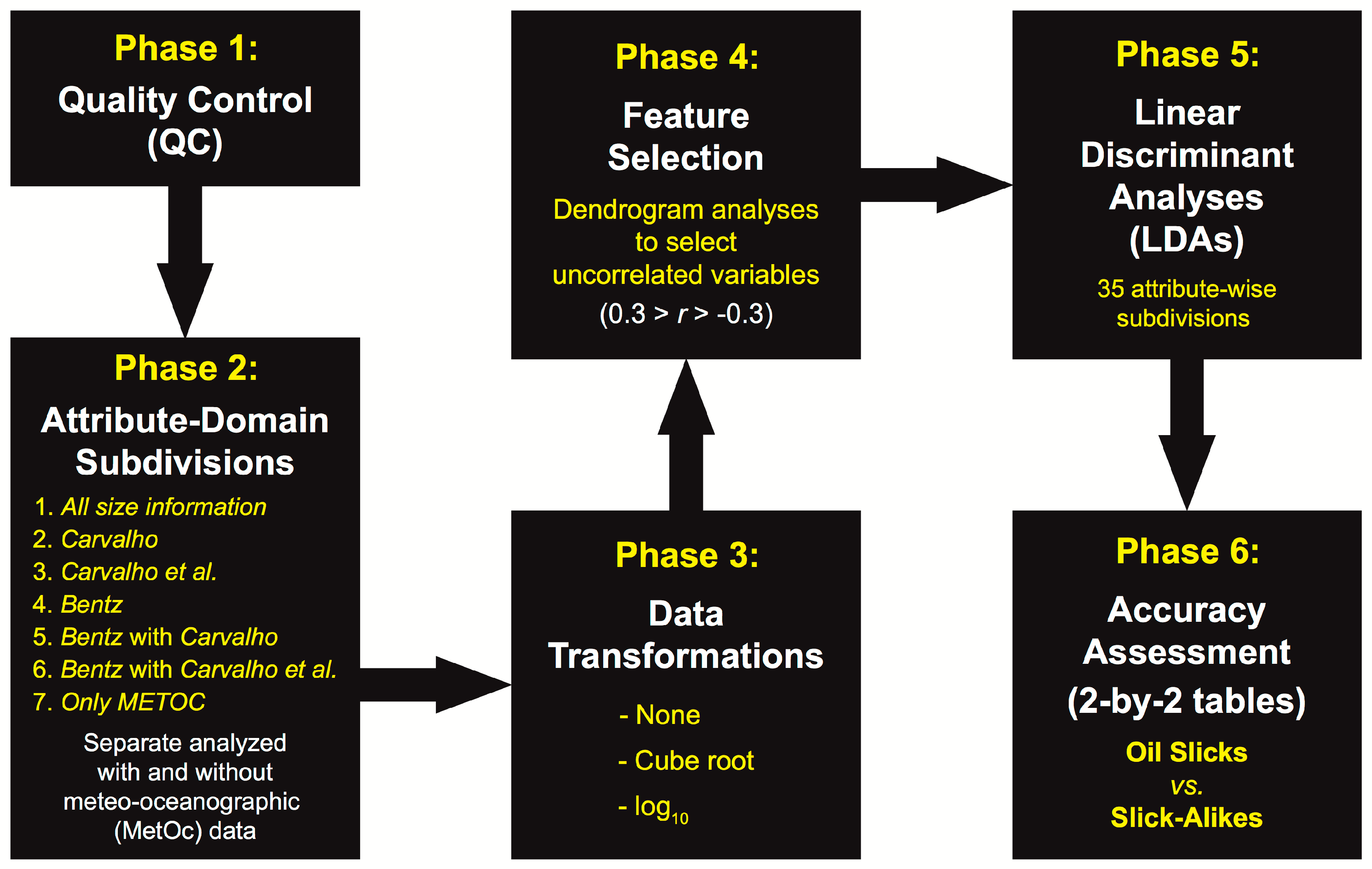
2.3. Research Strategy

A pictorial view of the research strategy explored to develop and evaluate our LDA algorithms is shown in Figure 3—quality control (QC), attribute–domain subdivisions, data transformations, feature selection, LDAs, and accuracy assessment. An open-access software package was used in our data mining exercises: PAST (PAleontological STatistics; [44,45]).

2.3.1. Phase 1: Quality Control (QC)

At the start, to certify that the database met certain effective conditions to accomplish the most accurate possible discrimination, we performed what we refer to as QC-standards:

• Verification of the reliability of the database records after data inconsistencies, i.e., removal of any sort of errors—for example, instances with missing value for any given attribute, obvious outliers, noisy data, etc.;
• Valuation of the attribute types to their suitability for our purposes; and
• Inspection of correlation matrices to avoid inter-correlation, as LDAs require the smallest correlation among the candidate variables [46].

2.3.2. Phase 2: Attribute–Domain Subdivisions

As in the seep-spill LDA differentiation discussed in Section 1.1, we followed the same pathways to investigate if there were combinations of variables that better discriminated oil from look-alikes. As such, after performing the QC’s, we divided the attribute set into various, small, specific subdivision domains based on the previous experiences of Carvalho [18,21] (Section 1.1.2), Carvalho et al. [22,23,24] (Section 1.1.3), and [17] (Section 2.2.2.1). Likewise, to inspect the influence of the MetOc information in this process, we performed separate analyses with and without the MetOc data.

2.3.3. Phase 3: Data Transformations

Carvalho et al. demonstrated that the LDA ability to discriminate oil (seeps) from oil (spills) is positively influenced by the application of non-linear transformations, i.e., cube root and log₁₀. Here, we compared the ability to distinguish oil slicks from slick-alikes using the original Campos Basin data with and without applying the two best data transformations they reported. This was done in all subdivisions defined in Phase 2.

2.3.4. Phase 4: Feature Selection

Commonly referred to as “feature engineering”, in which relevant attributes are selected to be applied in the classification system, this process also reduces the attribute dimensionality [47]. Hence, our feature selection consisted in the analyses of UPGMA dendrograms, separately carried out on each attribute–domain combination (Phase 2) in all data transformations (Phase 3). The interpretation of dendrograms is very simple. The level of which uncorrelated variables are selected is subjectively defined by the user. Visual analyses are a common practice, but generally, horizontal lines drawn across the dendrograms are used to form groups of correlated variables from which only one is selected to represent each group, ensuring there is no correlation among the selected variables—such lines are called phenon lines and are user-defined similarity cut-offs [48]. Here, to use as few correlated variables as possible in the LDA [46], we applied Pearson’s r correlation coefficients to define the level from which uncorrelated variables were selected: 0.3 > r > -0.3—see Section 1.1.3 [22,23,24].

2.3.5. Phase 5: Linear Discriminant Analyses (LDAs)

Because of the promising use of a linear, parametric, multivariate analysis method to automatically discriminate seeps from spills, as discussed above in Section 1.1, we also used LDAs to design an algorithm to identify two distinct categories: oil slicks vs. slick-alikes. LDAs have two main prerequisites:

• The candidate variables must have the least possible inter-correlation [46]—this has been addressed above (Phases 1 and 4); and
• The data must contain dichotomy information (in our case, oil and look-alikes) that is used to reach (and corroborate) the models’ classification accuracy—this is dealt with below (Phase 6), and indeed, these mutually exclusive a priori known labels are used to fine-tune our supervised learning application [49].

2.3.6. Phase 6: Accuracy Assessment

The LDAs performed in Phase 5 were individually evaluated with all 769 targets in the database of oil and look-alike slicks (Figure 2). By not withholding samples for a separate test set, we were able to obtain the best quality of circumstances to reach the least out-of-sample errors. Yet, utilizing all samples to train the classification model, the risk is incurred of having high training errors (i.e., our classification misidentifies too many targets), hence deeming our algorithms null and void. On the other hand, if obtaining low overall accuracy errors (i.e., our classification strikes most samples of both categories correctly), our model is successful.

The accuracy assessment of classification algorithms in data science investigations is generally quantified using confusion matrices, i.e., two-by-two tables [50]. In our matrices, the reference data are in the horizontal and the classified data in the vertical—in

Table 1. Confusion matrix (i.e., two-by-two table: A, B, C, and D) used to evaluate our Linear Discriminant Analyses (LDAs). The overall accuracy is expressed using the diagonal elements: (A+D)/(A+B+C+D).

	LDA oil slicks	LDA look-alikes	All known targets
Known oil slicks	A	B	A + B
Known look-alikes	C	D	C + D
All LDA targets	A + C	B + D	A + B + C + D
	LDA oil slicks	LDA look-alikes	All known targets
Known oil slicks	Correctly classified oil slicks	Miss classified oil slicks	All known oil slicks (i.e., 350)
Known look-alikes	Miss classified look-alikes	Correctly classified look-alikes	All known look-alikes (i.e., 419)
All LDA targets	All LDA classified oil slicks	All LDA classified look-alikes	All known targets (i.e., 769)

, rows are the a priori known classification and columns are the model outcome. A common metric to assess the correct classification of both categories is the overall accuracy, expressed as a percent. It is calculated by adding the diagonal elements of Table 1—i.e., correctly classified oil slicks (A) and correctly classified look-alikes (D)—then dividing it by the total number of samples; 769 in our case.

Nevertheless, the use of this metric alone may give the wrong impression about the true reliability of the algorithm [51,52,53]. This can be avoided by evoking supplementary statistical measures which are calculated from “horizontal” (

Table 2. “Horizontal” analysis of the confusion matrix shown in Table 1 with some of the supplementary measures used to evaluate our Linear Discriminant Analyses (LDAs).

	LDA oil slicks	LDA look-alikes	All known targets
Known oil slicks	A/(A+B)	B/(A+B)	(A+B)/(A+B)
Known look-alikes	C/(C+D)	D/(C+D)	(C+D)/(C+D)
	LDA oil slicks	LDA look-alikes	All known targets
Known oil slicks	Sensitivity	False negative	100%
Known look-alikes	False positive	Specificity	100%

) and “vertical” (

Table 3. “Vertical” analysis of the confusion matrix shown in Table 1 with some of the associated metrics used to evaluate our Linear Discriminant Analyses (LDAs).

	LDA oil slicks	LDA look-alikes
Known oil slicks	A/(A+C)	B/(B+D)
Known look-alikes	C/(A+C)	D/(B+D)
All LDA targets	(A+C)/(A+C)	(B+D)/(B+D)
	LDA oil slicks	LDA look-alikes
Known oil slicks	Positive predictive value	Inverse of the neg. pred. val.
Known look-alikes	Inverse of the pos. pred. val.	Negative predictive value
All LDA targets	100%	100%

) analyses of the confusion matrix (Table 1). The information given by these associated metrics is important to estimate how appropriate our discrimination models are. We chose to split the information in a separate schema to facilitate the comprehension of such metrics—see Table 1, Table 2 and Table 3. From Table 2 we obtain sensitivity and specificity, as well as their counterparts: false negatives and false positives. These inform how well the a priori known samples are classified (producer’s accuracy) and how badly the a priori known samples are misclassified (omission error or Type I error). Table 3 shows the positive and negative predictive values and their complements: inverse of the positive and negative predictive values. These report how well the models classify the actual samples (user’s accuracy) and how bad the algorithms misinterpret them (commission error or Type II error).

Because we are exploring several attribute–domain combinations (Phase 2), we represent our accuracy assessment in a “condensed” two-by-two cross-tabulation form—

Table 4. “Condensed” form of the confusion matrix shown in Table 1 used to access the classification accuracy of our Linear Discriminant Analyses (LDAs). See also Table 2 and Table 3.

Oil slicks		Look-alikes		All targets
A	A/(A+B)	D	D/(C+D)	A+D	(A+D)
	A/(A+C)		D/(B+D)		(A+B+C+D)
Oil slicks		Look-alikes		All targets
Correctly classified oil slicks	Sensitivity	Correctly classified look-alikes	Specificity	Correctly classified targets	Overall accuracy
	Positive predictive value		Negative predictive value

. This discloses in a single table the main metrics shown in Table 2 (sensitivity and specificity) and in Table 3 (positive and negative predictive values), along with the overall accuracy. Table 4 also provides a simplified, comparable-fashion presentation of the across-subdivision accuracy results of the classification algorithms.

3. Results

3.1. QC-Standards

In the first QC-standard, we identified ten data records having some inconsistency, most likely from typos: eight oil slicks and two slick-alike targets. These instances were removed from subsequent analysis. Consequently, after completing this first QC, the database has 769 targets: 350 oil slicks (45.5%) and 419 look-alike slicks (54.5%)—Figure 2.

The second QC-standard considered the utility of the attribute types describing the identified targets. Accordingly, because the values of the SAR-signature and textural information were calculated and registered in uncalibrated DNs, these attributes are not explored further here. The use of DNs for an analysis of measurement time series may mask important relationships, which may become more apparent by using calibrated measurements [18]. The attributes of location are also not employed in this investigation, as we intend to develop an algorithm that can be applied anywhere, and such site-specific variables cannot be transferred from one region to another. In addition, scene-related attributes are not included. Furthermore, due to the binary character of the cloud data (1 or 0), this MetOc descriptor is not considered here. After the application of this second QC, several irrelevant attribute types have been discarded, leaving only two attribute types to be carried forward: size information (Section 2.2.2.1) and contextual MetOc conditions (Section 2.2.2.2).

The inspection of the correlation matrices, the third QC-standard, revealed that some size variables are inter-correlated: SHP (shape index) with CMP (compact index), and ASY (asymmetry) with LtoW (length-to-width ratio). Authors in [22,23] also observed in the seep-spill dataset that SHP and CMP had an equal but inverted frequency distribution. From these four attributes, only two, CMP and LtoW, are used due to their simplicity. Additionally, based on earlier results [24], we have included two other size variables: PtoA and FRA. Therefore, based on the available variables within the database (Section 2.2.2.1; [17]) and on the LDA legacy left by [18,21,22,23,24] on their seep-spill discrimination, a specific set of nine size variables are used as follows:

• Area;
• Per: perimeter;
• PtoA: perimeter-to-area ratio;
• CMP: compact index;
• FRA: fractal index;
• LtoW: length-to-width ratio;
• DEN: density;
• CUR: curvature; and
• NUM: number of parts of each target.

The correlation matrices also confirmed inter-correlation among the three MetOc forms, i.e., the average values inside the polygons are correlated with the difference and ratio between the inside and outside of the polygons. As a result, only the more intuitive magnitude of the averaged values from inside the targets were retained:

• SST: sea surface temperature;
• CHL: concentration of chlorophyll-a; and
• WND: wind speed.

As such, the application of this third QC led to the initial data analyses using twelve descriptors: nine size attributes and three MetOc variables.

3.2. Attribute–Domain Subdivisions

The nine size variables determined by the QC’s were initially analyzed together; these are named “All size information”. They were then divided in different subdivisions grouped based on the earlier results of Carvalho [18,21] and Carvalho et al. [22,23,24] (Section 1.1.2 and Section 1.1.3, respectively), as well as on the variables previously given in [17]—the latter is simply referred to as “Bentz” (Section 2.2.2.1). Two additional combinations of variables are also investigated: “Bentz with Carvalho” and “Bentz with Carvalho et al.” From this point onwards, the terms Carvalho, Carvalho et al., and Bentz are also used to define the set of variables corresponding to each of these studies, as shown below. As a result, seven major attribute–domain combinations were proposed (color-coded in our plots and tables):

• All size information (n = 9), see Section 3.1;
• Carvalho (n = 2)—Area and Per;
• Carvalho et al. (n = 3)—PtoA, CMP, and FRA;
• Bentz (n = 4)—LtoW, DEN, CUR, and NUM;
• Bentz with Carvalho (n = 6);
• Bentz with Carvalho et al. (n = 7); and
• MetOc-Only (n = 3), see Section 3.1.

Additionally, all subdivisions were separately analyzed with and without the MetOc variables. As combinations in the attribute domain are analyzed with and without MetOc, as well as with the application of the three data transformations, there are 39 attribute subdivisions.

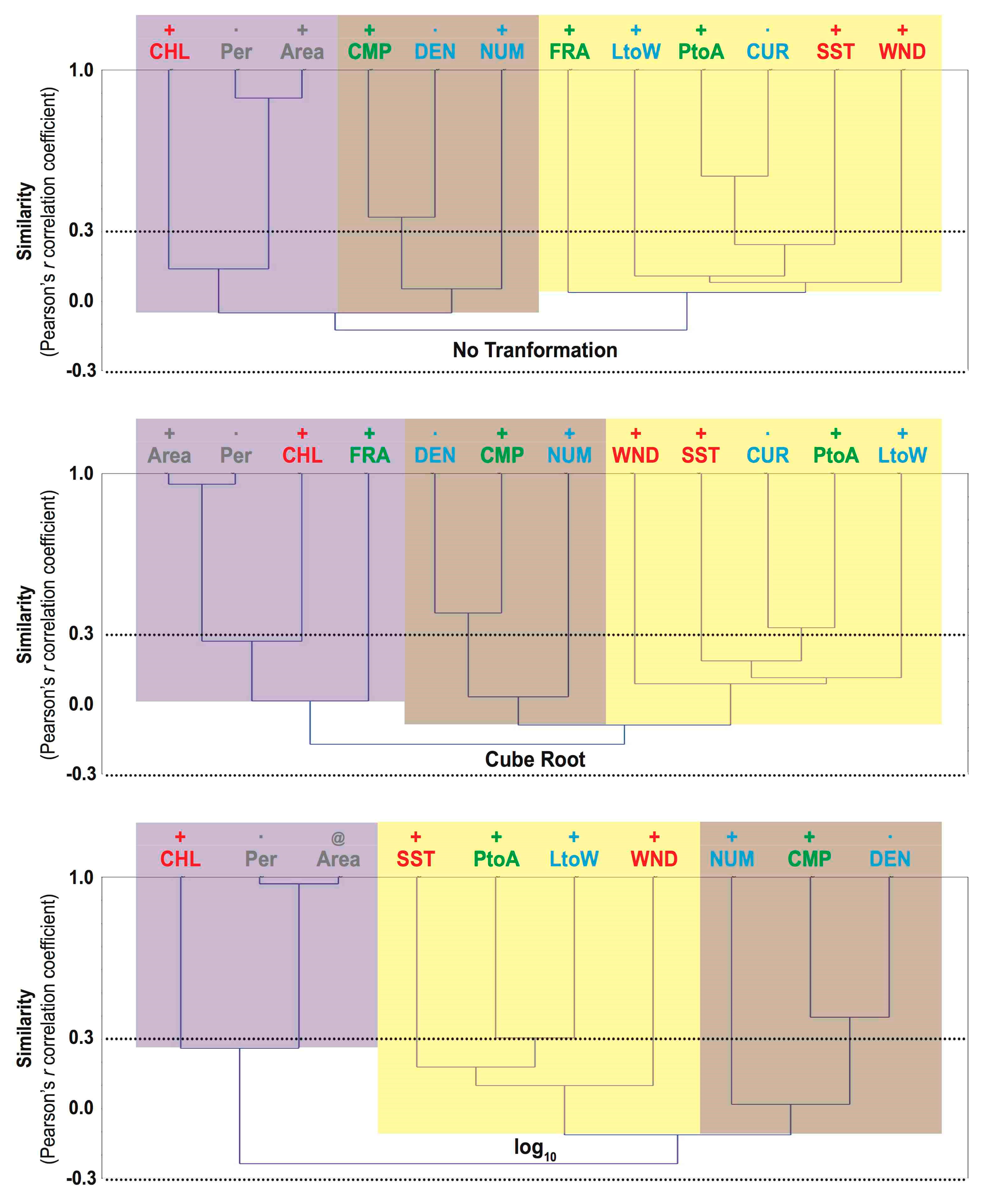
3.3. Feature Selection

Figure 4 presents the dendrograms for the different transformations (none, cube root, and log₁₀) applied to all twelve variables: All size information with MetOc. The two horizontal dotted lines correspond to the phenon lines: 0.3 > r > -0.3. The uncorrelated variables selected both with and without MetOc are represented with +, and those selected only with MetOc with @. Variables not explored further due to statistical correlation (0.3 < r < −0.3) are marked with a dot. The dendrograms of the other attribute–domain combinations (with and without MetOc) are similar to those in Figure 4.

A noteworthy characteristic of some variables shown in Figure 4 is that some variables are correlated (r > 0.3): CMP (compact index) with DEN (density), and PtoA (perimeter-to-area ratio) with CUR (curvature). From these four variables two were selected based on their simplicity: CMP and PtoA. These relationships similarly occur in the other subdivisions. Additionally, as in Carvalho’s seep-spill exercise, Area and perimeter (Per) are correlated here too, and from the two, we chose to retain Area. It is worth mentioning that in Carvalho, this pair of correlated morphological features had undergone a PCA before the values were input into their LDAs, i.e., PC scores instead of actual values.

Figure 4 (top panel: original data; and middle panel: cube root) indicates that of twelve attributes, nine are deemed uncorrelated (+); therefore, these were selected for input to the LDA for this subdivision: Area, PtoA, CMP, FRA, LtoW, NUM, SST, CHL, and WND; see also

Table 5. Feature selection outcome from the Unweighted Pair Group Method with Arithmetic Mean (UPGMA) dendrogram analyses performed on several attribute–domain subdivisions with three non-linear transformations (none, cube root, and log₁₀), with and without the Meteorological and Oceanographic ancillary information (MetOc): uncorrelated selected variables (Pearson’s correlation coefficient: 0.3 > r > −0.3) both with and without MetOc (+) and only with MetOc (@). Variables not explored per subdivision have an empty cell. Variables not selected due to statistical correlation (0.3 < r < −0.3) are marked with a dot. Gray subdivision (n = 2): “Carvalho” refers to [18,21], see Section 2.3.2. Green subdivision (n = 3): “Carvalho et al.” corresponds to [22,23,24], see Section 2.3.3. Blue subdivision (n = 4): “Bentz” is associated to [17]. Red subdivision (n = 4): MetOc-Only subdivision. Additional information on the origin of the variables subdivisions is found in Section 3.2 and Section 3.3. See text for color-coding used only to facilitate the visualization (Section 3.3.1). Explored variables (n = 12): Area; Per (perimeter); PtoA (perimeter-to-area ratio); CMP (compact index: 4.π.Area/Per²); FRA (fractal index: 2.ln(Per/4)/ln(Area)); LtoW (length-to-width ratio); DEN (density); CUR (curvature); NUM (number of parts); SST (sea surface temperature); CHL (chlorophyll-a concentration); and WND (wind speed). See Figure 4 for graphical representations of the All size information with MetOc subdivisions.

Selected Variables (+ and @): Uncorrelated if 0.3 > r > -0.3		Size Information (n = 9)									MetOc (n = 3)			Selected Variables (uncorrelated) out of Explored Variables
		“Carvalho“		“Carvalho et al.”			“Bentz”
Subdivisions	Transformations	Area	Per	PtoA	CMP	FRA	LtoW	DEN	CUR	NUM	SST	CHL	WND	Without MetOc	With MetOc
1.“All size information“	None	+	.	+	+	+	+	.	.	+	@	@	@	6 out of 9	9 out of 12
	Cube root	+	.	+	+	+	+	.	.	+	@	@	@	6 out of 9	9 out of 12
	log10	@	.	+	+		+	.		+	@	@	@	4 out of 7	8 out of 10
2. Carvalho	None	@	.								@	@	@	0 out of 2	4 out of 5
	Cube root	@	.								@	@	@	0 out of 2	4 out of 5
	log10	@	.								@	@	@	0 out of 2	4 out of 5
3. Carvalho et al.	None			+	+	+					@	@	@	3 out of 3	6 out of 6
	Cube root			+	+	+					@	@	@	3 out of 3	6 out of 6
	log10			@	.						@	@	@	0 out of 2	4 out of 5
4. Bentz	None						@	+	+	+	@	@	@	3 out of 4	7 out of 7
	Cube root						@	+	+	+	@	@	@	3 out of 4	7 out of 7
	log10						@	+		+	@	@	@	2 out of 3	6 out of 6
5. Bentz with Carvalho	None	+	.				+	+	+	+	@	@	@	5 out of 6	8 out of 9
	Cube root	+	.				+	+	+	+	@	@	@	5 out of 6	8 out of 9
	log10	+	.				+	+		+	@	@	@	4 out of 5	7 out of 8
6. Bentz with Carvalho et al.	None			+	+	+	+	.	.	+	@	@	@	5 out of 7	8 out of 10
	Cube root			+	+	+	+	.	.	+	@	@	@	5 out of 7	8 out of 10
	log10			+	+		+	.		+	@	@	@	4 out of 5	7 out of 8
7. MetOc-Only	None										@	@	@		3 out of 3
	Cube root										@	@	@		3 out of 3
	log10										@	@	@		3 out of 3

. The three eliminated variables are marked with a dot: Per, DEN, and CUR. These three correlated variables are redundant for the purposes of using LDAs as they do not bring independent information. A remarkable aspect about the log₁₀ transformation (Figure 4: bottom panel) is that when it is applied, only ten variables are included in this subdivision, from which eight are selected: + or @. This is because FRA and CUR may have negative values and, thus, cannot be accounted with this transformation; some subdivisions do not consider these two variables: Carvalho and MetOc-Only (Table 5).

Table 5 presents the variables selected with the UPGMA dendrograms for the 39 attribute subdivision domains. Four main aspects are apparent in this table:

• There is a considerable reduction in the attribute dimensionality in all combinations of attributes;
• Whenever the three MetOc variables are considered, they are always selected, including the MetOc-Only subdivision;
• Among all attribute–domain subdivisions, the number of selected (uncorrelated) variables ranges from two to nine; and
• In four subdivisions (i.e., Carvalho in the three transformations and Carvalho et al. with log₁₀; all without MetOc) the attributes are correlated, and as such are not selected.

From this last aspect, of the 39 proposed feature selection evaluations, 35 different LDAs were performed.

3.3.1. Dendrogram Visual Inspection

Notwithstanding the use of phenon lines, the visual analyses of our UPGMA dendrograms usually reveal that specific groups of variables are formed independent of data transformation, see Figure 4 (these are color-coded: purple, brown, and yellow). Nevertheless, these visually-combined variables should not be confused with those selected with the similarity lines: 0.3 > r > -0.3 (Table 5). In fact, such visual grouping of attributes is not critical to this analysis, but this comes to prominence because these color-groups show some unusual relationships among the attributes. The groups are:

• Purple: Area and Per form a group with CHL;
• Brown: CMP, DEN, and NUM form another separate group; and
• Yellow: PtoA, FRA, LtoW, and CUR tend to group with SST and WND.

Minor variations are observed in these groupings across the other attribute–domain combinations. These visually-identified groups of variables are linked to each other at levels close to zero similarity (r ~ 0), meaning that there is almost no inter-group correlation (Figure 4).

3.4. Accuracy Assessment

Table 6. Classification accuracies of the 35 different LDA algorithms. See also Table 1, Table 2, Table 3, Table 4 and Table 5. The plots for the three All size information with MetOc subdivisions (bold) are shown in Figure 4.

Hierarchy	Subdivisions	Variables	Transformations	MetOc	Oil Slicks		Look-Alikes		All Targets
1	5. Bentz with Carvalho	7 out of 8	log10	With	316	90.3%	328	78.3%	644	83.7%
						77.6%		90.6%
2	1. All size information	9 out of 12	Cube root	With	309	88.3%	335	80.0%	644	83.7%
						78.6%		89.1%
3	6. Bentz with Carvalho et al.	8 out of 10	Cube root	With	315	90.0%	326	77.8%	641	83.4%
						77.2%		90.3%
4	6. Bentz with Carvalho et al.	7 out of 8	log10	With	315	90.0%	325	77.6%	640	83.2%
						77.0%		90.3%
5	1. All size information	9 out of 12	None	With	305	87.1%	334	79.7%	639	83.1%
						78.2%		88.1%
6	6. Bentz with Carvalho et al.	8 out of 10	None	With	304	86.9%	334	79.7%	638	83.0%
						78.1%		87.9%
7	1. All size information	8 out of 10	log10	With	315	90.0%	323	77.1%	638	83.0%
						76.6%		90.2%
8	5. Bentz with Carvalho	8 out of 9	Cube root	With	321	91.7%	311	74.2%	632	82.2%
						74.8%		91.5%
9	2. Carvalho	4 out of 5	log10	With	310	88.6%	308	73.5%	618	80.4%
						73.6%		88.5%
10	5. Bentz with Carvalho	8 out of 9	None	With	303	86.6%	315	75.2%	618	80.4%
						74.4%		87.0%
11	4. Bentz	7 out of 7	Cube root	With	299	85.4%	318	75.9%	617	80.2%
						74.8%		86.2%
12	3. Carvalho et al.	6 out of 6	Cube root	With	306	87.4%	309	73.7%	615	80.0%
						73.6%		87.5%
13	4. Bentz	6 out of 6	log10	With	299	85.4%	315	75.2%	614	79.8%
						74.2%		86.1%
14	3. Carvalho et al.	4 out of 5	log10	With	309	88.3%	303	72.3%	612	79.6%
						72.7%		88.1%
15	3. Carvalho et al.	6 out of 6	None	With	287	82.0%	323	77.1%	610	79.3%
						74.9%		83.7%
16	2. Carvalho	4 out of 5	Cube root	With	308	88.0%	300	71.6%	608	79.1%
						72.1%		87.7%
Hierarchy	Subdivisions	Variables	Transformations	MetOc	Oil slicks		Look-alikes		All targets
18	6. Bentz with Carvalho et al.	5 out of 7	None	Without	279	79.7%	329	78.5%	608	79.1%
						75.6%		82.3%
19	1. All size information	6 out of 9	None	Without	284	81.1%	324	77.3%	608	79.1%
						74.9%		83.1%
20	6. Bentz with Carvalho et al.	5 out of 7	Cube root	Without	292	83.4%	315	75.2%	607	78.9%
						73.7%		84.5%
21	1. All size information	6 out of 9	Cube root	Without	291	83.1%	316	75.4%	607	78.9%
						73.9%		84.3%
22	5. Bentz with Carvalho	4 out of 5	log10	Without	295	84.3%	307	73.3%	602	78.3%
						72.5%		84.8%
23	6. Bentz with Carvalho et al.	4 out of 5	log10	Without	295	84.3%	305	72.8%	600	78.0%
						72.1%		84.7%
24	1. All size information	4 out of 7	log10	Without	295	84.3%	305	72.8%	600	78.0%
						72.1%		84.7%
25	5. Bentz with Carvalho	5 out of 6	Cube root	Without	306	87.4%	289	69.0%	595	77.4%
						70.2%		86.8%
Hierarchy	Subdivisions	Variables	Transformations	MetOc	Oil slicks		Look-alikes		All targets
26	7. MetOc-Only	3 out of 3	Cube root	With	290	82.9%	303	72.3%	593	77.1%
						71.4%		83.5%
27	7. MetOc-Only	3 out of 3	None	With	277	79.1%	314	74.9%	591	76.9%
						72.5%		81.1%
28	2. Carvalho	4 out of 5	None	With	283	80.9%	308	73.5%	591	76.9%
						71.8%		82.1%
29	7. MetOc-Only	3 out of 3	log10	With	287	82.0%	303	72.3%	590	76.7%
						71.2%		82.8%
Hierarchy	Subdivisions	Variables	Transformations	MetOc	Oil slicks		Look-alikes		All targets
30	5. Bentz with Carvalho	5 out of 6	None	Without	279	79.7%	285	68.0%	564	73.3%
						67.6%		80.1%
31	3. Carvalho et al.	3 out of 3	None	Without	245	70.0%	314	74.9%	559	72.7%
						70.0%		74.9%
32	3. Carvalho et al.	3 out of 3	Cube root	Without	276	78.9%	279	66.6%	555	72.2%
						66.3%		79.0%
33	4. Bentz	3 out of 4	None	Without	254	72.6%	292	69.7%	546	71.0%
						66.7%		75.3%
34	4. Bentz	3 out of 4	Cube root	Without	251	71.7%	287	68.5%	538	70.0%
						65.5%		74.4%
35	4. Bentz	2 out of 3	log10	Without	278	70.9%	283	65.2%	521	67.8%
						62.9%		72.8%

presents the classification accuracies of the 35 different LDA-based algorithms; these are ordered by the results of the associated statistical metrics shown in Table 4—i.e., overall accuracy (diagonal analysis of Table 1), sensitivity and specificity (horizontal analysis of Table 2, producer’s accuracy), and positive and negative predictive values (vertical analysis of Table 3, user’s accuracy). Because we have 769 targets, the discretization interval of our analyses is 0.13%, i.e., 1/769.

The best discrimination uses Bentz (LtoW, DEN, and NUM) with Carvalho (Area) with MetOc (SST, CHL, and WND) with log₁₀ attribute subdivision (Table 6). A successful overall discrimination accuracy of 83.7% is observed when these seven descriptors are analyzed together: 644 samples are correctly identified (316 oil slicks and 328 slick-alikes: sensitivity of 90.3% and a specificity of 78.3%, with good levels of positive (77.6%) and negative (90.6%) predictive values). On the other hand, the least accurate attribute subdivision is Bentz (DEN and NUM) without MetOc with log₁₀ transformation (Table 6). The overall accuracy achieved when only these two attributers are used is as low as 67.8% (521 samples correctly identified: 248 oil slicks and 273 look-alikes) with sensitivity (70.9%), specificity (65.2%), and positive (62.9%) and negative (72.8%) predictive values.

Another notable characteristic observed in Table 6 is that there are four main hierarchy blocks been formed with similar attribute–domain combinations as a function of attribute types (i.e., size information with or without MetOc variables, as well as MetOc by itself):

• The top seventeen ranks from the subdivisions with MetOc;
• Eight ranks from the subdivisions without MetOc;
• The three MetOc-Only subdivisions, and another Carvalho subdivision (Area) with the three MetOc variables and no transformation (hierarchy #28 of Table 6); and
• The remaining six subdivisions without MetOc.

These results show the synergy that occurs whenever size variables are analyzed together with the MetOc information (1st hierarchy block of Table 6). It is noteworthy the superiority of some subdivisions that only account for the size variables without MetOc (2nd hierarchy block) over the sole use of the MetOc variables (3rd hierarchy block, i.e., MetOc-Only).

Table 7. Typical values of the four hierarchy blocks of Table 6: Average (Avg), Maximum (Max), Minimum (Min), and Standard Deviation (Std).

Typical Values		Size with MetOc		Size without MetOc		MetOc-Only		Size without MetOc
		1st block		2nd block		3rd block		4th block
Overall Accuracy	Avg	81.4%		78.5%		76.9%		71.2%
	Max	83.7%		79.1%		77.1%		73.3%
	Min	79.1%		77.4%		76.7%		67.8%
	Std	1.8%		0.6%		0.2%		2.1%
Sensitivity	Avg	87.6%		83.5%		81.2%		74.0%
	Max	91.7%		87.4%		82.9%		79.7%
	Min	82.0%		79.7%		79.1%		70.0%
Specificity	Avg	76.1%		74.3%		73.3%		68.8%
	Max	80.0%		78.5%		74.9%		74.9%
	Min	71.6%		69.0%		72.3%		65.2%
Positive Predictive Value	Avg	75.4%		73.1%		71.7%		66.5%
	Max	78.6%		75.6%		72.5%		70.0%
	Min	72.1%		70.2%		71.2%		62.9%
Negative Predictive Value	Avg	88.1%		84.4%		73.3%		68.8%
	Max	91.5%		86.8%		74.9%		74.9%
	Min	83.7%		82.3%		72.3%		65.2%
Subdivisions		Size with MetOc		Size without MetOc		MetOc-Only		Size without MetOc
		1st block		2nd block		3rd block		4th block
All size information		3	17.6%	3	37.5%	0	0.0%	0	0.0%
Carvalho		2	11.8%	0	0.0%	1	25.0%	0	0.0%
Carvalho et al.		3	17.6%	0	0.0%	0	0.0%	2	33.3%
Bentz		3	17.6%	0	0.0%	0	0.0%	3	50.0%
Bentz with Carvalho		3	17.6%	2	25.0%	0	0.0%	1	16.7%
Bentz with Carvalho et al.		3	17.6%	3	37.5%	0	0.0%	0	0.0%
MetOc-Only						3	75.0%
Data Transformations		Size with MetOc		Size without MetOc		MetOc-Only		Size without MetOc
		1st block		2nd block		3rd block		4th block
None		5	29.4%	2	25.0%	2	50.0%	3	50.0%
Cube Root		6	35.3%	3	37.5%	1	25.0%	2	33.3%
log10		6	35.3%	3	37.5%	1	25.0%	1	16.7%

(top) presents the typical values of the hierarchy blocks: mean, maximum, minimum, and standard deviation values. Again, the synergy of using size and MetOc simultaneously is observed in all given metrics. The averaged overall accuracies are: 81.4%, 78.5%, 76.9%, and 71.2%, respectively, for the four blocks. Likewise, the other associated statistical measures also follow this top-down sequence.

Table 7 (middle) shows that the top 17 ranks (i.e., 1st block) are formed by essentially an even number of combinations, i.e., each of the six major subdivisions correspond to ~17%. The next eight ranks (i.e., 2nd block) are also represented by a uniform number of subdivisions, i.e., ~30% of each: All size information (all transformations), Bentz with Carvalho (two transformations), and Bentz with Carvalho et al. (all transformations). While the 3rd block is represented by all three MetOc-Only subdivisions (75%) and Carvalho with MetOc (25%), the six ranks of the lower 4th block refers to Bentz in all transformations (50%), Carvalho et al. (~33%), and Bentz with Carvalho in two transformations (~17%).

Table 7 (bottom) reveals the absence of a direct benefit of applying non-linear transformations. In the top two blocks, there is a similar representativeness of all transformations (~30%), and in the lower two blocks the original data accounts for 50% of each. Furthermore, Table 6 reveals that there is no clear pattern in the ability of the LDA to discriminate between oil slicks and slick-alikes involving data transformations—both the top (83.7%) and worst (67.8%) overall accuracies are achieved with the same log₁₀ transformation.

4. Discussion

The knowledge gained from Carvalho [18,21] (Section 1.1.2) and Carvalho et al. [22,23,24] (Section 1.1.3) on the use of LDAs led us to apply such linear techniques in this study (Figure 3). A three-fold correspondence (similarities vs. differences) can be drawn between the earlier investigation and this study:

• Distinct categories of targets can be analyzed: the earlier studies were directed at the classification of mineral oil slick products (oil seeps vs. oil spills), but here the focus is on differentiating two types of low radar backscatter signals (oil slicks vs. slick-alikes);
• Different SAR dual co-polarizations measurements can be exploited: their SAR-derived smooth texture polygons were digitally classified with VV-polarized, 16-bit scenes (RADARSAT-2), but the database in this study was derived from HH-polarized, 8-bit imagery (RADARSAT-1); and
• Samples can come from different geographic places: the seep-spill effective discrimination was accomplished with oil slicks observed in the Gulf of Mexico, whereas here we analyzed targets from the offshore southeastern Brazilian coast (Figure 1).

Despite the success of linear discriminant multivariate analyses in these two domains—i.e., to separate oil from oil (e.g., [18]) and oil from look-alikes—one should bear in mind complementary non-linear machine learning models [54].

Additionally, there are three relevant aspects of the database used here:

• It includes interpretations by experts that have been supported by ancillary MetOc data [17]. The accuracy assessment of the LDA algorithms is compared to these man-made interpretations;
• This study used RADARSAT-1 data simply because a tabular database was available. The use of ship-based multi-band radars (e.g., X-/C-/S-band [55]) or a finer-resolution C-band SAR sensor (e.g., Sentinel-1s [56]) may result in more detailed analyses of small marine slicks; and
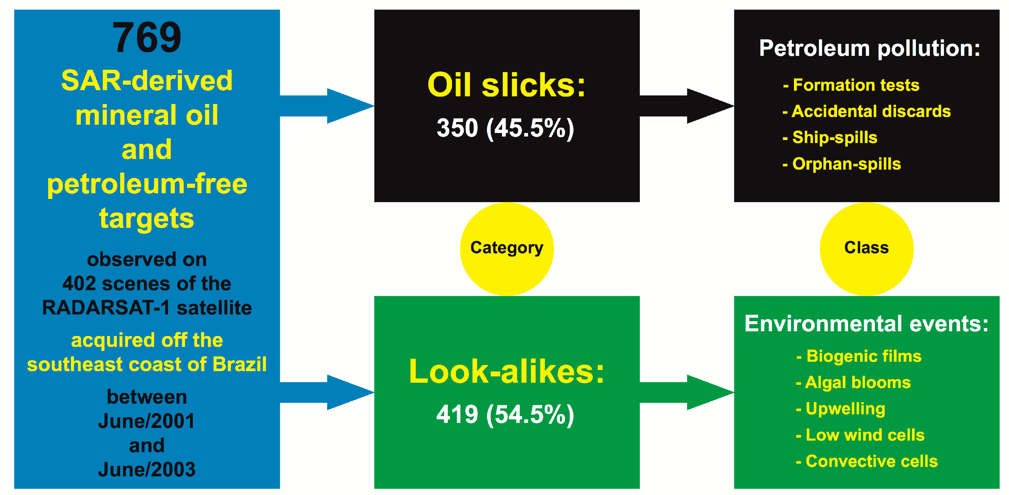
• The 402 scenes were sampled at about four images per week (between July 2001 and June 2003), thus registering the extremely high MetOc variability of the Campos Basin, and providing a large and quite well-balanced class distribution (Figure 2) of 350 petroleum pollution records (exploration and production oil, ship- and orphan-spills) versus 419 non-petroleum targets (biogenic films, algal blooms, upwelling, low wind, or rain cells). This sampling rate ensured that a wide range of conditions of various factors influencing the detection of oil slicks in SAR imagery (e.g., sea conditions, SAR noise floor, incidence angle, etc.; such aspects were not directly measured) were well represented.

As a result, this data representativeness ensures the database used is appropriate to train algorithms, thus supporting the investigation of a worldwide, economically relevant offshore region with major oil and gas resources, the Campos Basin, with known oil slick occurrence.

The QC standards guaranteed effective criteria to promote the discrimination between oil slicks and non-petroleum signals. Some attribute types (e.g., SAR-signature and textural information) were eliminated from this study because they were provided in uncalibrated DNs, which were not converted to backscatter coefficients (gamma-, beta-, or sigma-naught) given in amplitude or decibels [57]. Notwithstanding that Carvalho and Carvalho et al. showed the sole use of size information is sufficient to discriminate seeps from spills, their results were slightly improved when size and SAR descriptors were combined. Thus, the inclusion of SAR-signature and textural information given in terms of backscatter coefficients could imply further developments to our LDA discrimination process.

When Carvalho included site-specific attributes—latitude, longitude, and others—the discrimination was considerably improved to almost 100% accuracy. Here, location was not used as a parameter in the analysis so that a set of attributes and related algorithms could be derived suitable for application to signals in any area. However, in the development of an algorithm intended for a given region, the inclusion of location descriptors may be beneficial.

From the best 17 combinations of attributes (1st block in Table 6: size with MetOc variables), there is a difference in accuracy of 4.6% from the 1st to the 17th rank (644-608 = 36 correctly identified targets; Table 6 and Table 7). This means that the analyses of fixed specific subdivision domains could possibly be further developed with a one-to-one attribute substitution, i.e., having as many subdivisions as the number of possible combinations of variables, thus measuring the individual relevance per attribute. With such a procedure, a finer sense of which attribute combination best discriminates oil slicks from petroleum-free targets could be derived.

Our classification results are independent of the data transformation—i.e., original data, cube root, and log₁₀ (Table 6 and Table 7). Nevertheless, other non-linear transformations may result in improvements in the LDA oil and look-alike discrimination with, for instance, reciprocal, square root, square power, or cube power. Carvalho et al. tested these transformations, along with cube root and log₁₀, to find that the latter two achieved improved seep-spill discrimination.

To fulfill the LDA prerequisite of having the least correlation [46], our feature selection processes used UPGMA dendrograms with the similarity cut-off of 0.3 > r > -0.3 (Section 2.3.4: Phase 4). Nonetheless, visual inspections of dendrograms could be used instead (Section 3.3.1). In Figure 4 (any panel) three main groups of variables are formed with almost no inter-group correlation. These visually combined, uncorrelated groups of variables could be used to select one attribute from each group instead of using a fixed phenon line—for instance, in Figure 4, one could choose CHL from the purple group, CMP from the brown group, and SST from the yellow group. This would further trim the dimensionality, as instead of using nine variables out of the initial twelve (Table 5), only three attributes would be input into the LDA.

It is noteworthy that the three least accurate combinations (Bentz without MetOc in all transformations) are those using the four most complex of the nine size variables, i.e., LtoW, DEN, CUR, and NUM (Table 6). While this last variable can be simply achieved by counting the number of parts of each low backscatter SAR target, the other three require more complicated calculations than the other five size explored variables, i.e., Area and Per (Carvalho), along with PtoA, CMP, and FRA (Carvalho et al.). The latter three attributes are straightforward to derive from the first two, i.e., the most basic morphological characteristics of the polygons. This demonstrates that simple descriptors can result in successful oil and look-alike discrimination, as was also found by Carvalho and Carvalho et al. while discriminating seeps from spills.

The interplay between size and MetOc variables observed on the accuracy assessment results in four hierarchy blocks (Table 6). Table 7 shows that, on average, even the attribute–domain combinations of the least accurate hierarchy block upheld practical accuracies of about 70% in all of the metrics, meaning that they can still be considered useful algorithms.

5. Conclusions

The discrimination of two categories of low-backscatter regions derived from Synthetic Aperture Radar (SAR) measurements (i.e., mineral oil slicks and other environmental petroleum-free false targets—oil vs. look-alikes) has been demonstrated. These two low-backscatter categories have been distinguished with simple, parametric Linear Discriminant Analyses (LDAs) applied to a set of satellite measurements (microwave, infrared, and optical) from RADARSAT-1, AVHRR/NOAA, SeaWiFS/Orbiview-2, MODIS/Terra, and SeaWinds/QuikSCAT. The study region, the Campos Basin (Figure 1), is located off the southeast coast of Brazil, and our database consists of 769 samples of oil slicks (n = 350; 45.5%) and slick-alikes (n = 419; 54.5%) derived from 402 RADARSAT-1 scenes from July 2001 to June 2003 (Figure 2). The LDA algorithms were evaluated with a three-fold statistical metric: overall, producer’s and user’s accuracies (Table 1, Table 2, Table 3 and Table 4). The investigation plan (Figure 3) involved the evaluation of 39 attribute subdivisions based on the knowledge gained from the earlier seep-spill discrimination findings of “Carvalho” [18,21] (Section 1.1.2), “Carvalho et al.” [22,23,24] (Section 1.1.3), as well as from “Bentz” [17] (Section 2.2.2.1)—Table 5. Therefore, evoking the assistance of Figure 4 and Table 6 and Table 7, the initial six questions have been answered:

• This research has shown that oil slicks and radar look-alikes are distinguishable by means of a simple linear, but mathematically-robust, multivariate data analysis technique, LDA.
• The LDA algorithms achieved classification accuracies that support further, systematic implementation (commercially or academically), as the best overall classification accuracies of ~80% with good levels of sensitivity (~90%), specificity (~80%), positive (~80%) and negative (~90%) predictive values have been demonstrated.
• The application of non-linear transformations does not result in improvement in the discrimination of oil slicks and look-alike signals. In fact, both the best and worst accuracies (83.7% and 67.3%) were achieved using the same transformation: log₁₀, as expected from the seep-spill discrimination findings of Carvalho et al.
• It has been demonstrated that the exclusive use of the magnitude of contextual Meteorological-Oceanographic (MetOc) satellite-derived variables (sea surface temperature (SST), chlorophyll-a (CHL), and wind speed (WND)) is sufficient to distinguish oil slicks from false targets. The best classification accuracy using solely MetOc variables (with the cube root transformation applied) is 77.1%.
• A specific set of attributes was selected to be used in our analyses after the legacy left from the seep-spill discrimination [18,21,22,23,24], so as by the available variables within the database [17] (Table 5). From these, several attribute combinations were tested and led to similar discriminations of oil slicks and slick-alikes: most of the top 17 attribute subdivisions resulted in an overall accuracy > 80%. Thus, “the best” selection of variables cannot be specified, as we did not test all possible combinations of variables. Nevertheless, among the 39 attribute subdivisions tested, the most reliable discrimination (overall accuracy of 83.7%) has seven descriptors: Area, length-to-width ratio (LtoW), density (DEN), number of parts of each target (NUM), and the magnitudes of SST, CHL, and WND—i.e., the Bentz with Carvalho with MetOc with log₁₀ subdivision. The worst discrimination only accounts for two variables: DEN and NUM (67.8% of overall accuracy—i.e., Bentz without MetOc with log₁₀).
• The set-up of our LDA-based algorithm is most likely not site-specific, and indeed it could be applied to other regions. However, the applicability of the algorithms should be confirmed if a local training dataset is available. If such a dataset is available, and our algorithm is found not to be sufficiently effective, then the approach presented here could be followed to generate a more locally appropriate algorithm.

This study has produced an approach to perform offshore monitoring of marine oil slicks using satellite data, resulting in an easy research-to-application transition. These results substantiate that discrimination between mineral oil slicks and environmental petroleum-free look-alike slicks can be accomplished effectively with simple linear discriminant multivariate analyses.

References

1. Figueiredo, M.G.; Alvarez, D.; Adams, R.N. Revisiting the P-36 oil rig accident 15 years later: From management of incidental and accidental situations to organizational factors. Cadernos de Saúde Pública 2018, 34, e00034617. [Google Scholar] [CrossRef] [PubMed] [Green Version]
2. Forbes. 2001. Available online: https://www.forbes.com/2001/03/19/0319disaster.html (accessed on 5 June 2020).
3. BBC. 2019. Available online: https://www.bbc.com/news/world-latin-america-50223106 (accessed on 5 June 2020).
4. New York Times. 2019. Available online: https://www.nytimes.com/2019/10/08/world/americas/brazil-oil-spill-beaches.html (accessed on 5 June 2020).
5. CNN. 2019. Available online: https://edition.cnn.com/2019/10/09/americas/brazil-oil-spill-intl/index.html (accessed on 5 June 2020).
6. The Guardian. 2019. Available online: https://www.theguardian.com/world/2019/nov/01/brazil-blames-oil-spill-greek-flagged-tanker-venezuelan-crude (accessed on 5 June 2020).
7. Holt, B. SAR imaging of the ocean surface. In Synthetic Aperture Radar Marine User’s Manual, NOAA/NESDIS; Jackson, C.R., Apel, J.R., Eds.; Office of Research and Applications: Washington, DC, USA, 2004; Chapter 2; pp. 25–79. [Google Scholar]
8. Ufermann, S.; Robinson, I.S.; da Silva, J.C.B.D. Synergy between synthetic aperture radar and other sensors for the remote sensing of the ocean. Annales Des Télécommunications 2001, 56, 672–681. [Google Scholar] [CrossRef]
9. Ivonin, D.; Brekke, C.; Skrunes, S.; Ivanov, A.; Kozhelupova, N. Mineral Oil Slicks Identification Using Dual Co-polarized Radarsat-2 and TerraSAR-X SAR Imagery. Remote Sens. 2020, 12, 1061. [Google Scholar] [CrossRef] [Green Version]
10. Stringer, W.J.; Ahlnas, K.; Royer, T.C.; Dean, K.E.; Groves, J.E. Oil spill shows on satellite image, EOS Transactions. Am. Geophys. Union. 1989, 70, 564. [Google Scholar] [CrossRef]
11. Banks, S. SeaWiFS satellite monitoring of oil spill impact on primary production in the Galapagos Marine Reserve. Mar. Pollut. Bull. 2003, 47, 325–330. [Google Scholar] [CrossRef]
12. Bulgarelli, B.; Djavidnia, S. On MODIS retrieval of oil spill spectral properties in the marine environment. IEEE Geosci.Remote Sens. Lett. 2012, 9, 398–402. [Google Scholar] [CrossRef]
13. Alpers, W.; Holt, B.; Zeng, K. Oil spill detection by imaging radars: Challenges and pitfalls. Remote Sens. Environ. 2017, 201, 133–147. [Google Scholar] [CrossRef]
14. Martin, S. An Introduction to Ocean Remote Sensing, 1st ed.; Cambridge University Press: Cambridge, UK, 2004; 426p, ISBN 0-521-80280-6. [Google Scholar]
15. Espedal, H.A.; Johannessen, O.M. Detection of Oil Spills Near Offshore Installations Using Synthetic Aperture Radar (SAR). Int. J. Remote Sens. 2000, 21, 2141–2144. [Google Scholar] [CrossRef]
16. Genovez, P.C. Segmentação e Classificação de Imagens SAR Aplicadas à Detecção de Alvos Escuros em Áreas Oceânicas de Exploração e Produção de Petróleo. Ph.D. Thesis, COPPE, Universidade Federal do Rio de Janeiro (UFRJ), Rio de Janeiro, Brazil, 2010; 235p. [Google Scholar]
17. Bentz, C.M. Reconhecimento Automático de Eventos Ambientais Costeiros e Oceânicos em Imagens de Radares Orbitais. Ph.D. Thesis, COPPE, Universidade Federal do Rio de Janeiro, UFRJ), Rio de Janeiro, Brazil, 2006; 115p. [Google Scholar]
18. Carvalho, G.A. Multivariate Data Analysis of Satellite-Derived Measurements to Distinguish Natural from Man-Made Oil Slicks on the Sea Surface of Campeche Bay (Mexico). Ph.D. Thesis, COPPE, Universidade Federal do Rio de Janeiro (UFRJ), Rio de Janeiro, Brazil, 2015; 285p. Available online: http://www.coc.ufrj.br/pt/teses-de-doutorado/390-2015/4618-gustavo-de-araujo-carvalho (accessed on 5 June 2020).
19. Garcia-Pineda, O.; Zimmer, B.; Howard, M.; Pichel, W.; Li, X.; MacDonald, I.R. Using SAR images to delineate ocean oil slicks with a texture classifying neural network algorithm (TCNNA). Can. J. Remote Sens. 2009, 35, 11. [Google Scholar] [CrossRef]
20. Krestenitis, M.; Orfanidis, G.; Ioannidis, K.; Avgerinakis, K.; Vrochidis, S.; Kompatsiaris, I. Oil Spill Identification from Satellite Images Using Deep Neural Networks. Remote Sens. 2019, 11, 1762. [Google Scholar] [CrossRef] [Green Version]
21. Carvalho, G.A.; Minnett, P.J.; de Miranda, F.P.; Landau, L.; Paes, E.T. Exploratory data analysis of synthetic aperture radar (SAR) measurements to distinguish the sea surface expressions of naturally-occurring oil seeps from human-related oil spills in Campeche Bay (Gulf of Mexico). ISPRS Int. J. Geo. Inf. 2017, 6, p379. [Google Scholar] [CrossRef] [Green Version]
22. Carvalho, G.A.; Minnett, P.J.; Paes, E.T.; Miranda, F.P.; Landau, L. Refined analysis of RADARSAT-2 measurements to discriminate two petrogenic oil-slick categories: Seeps versus spills. J. Mar. Sci. Eng. 2018, 6, 153. [Google Scholar] [CrossRef] [Green Version]
23. Carvalho, G.A.; Minnett, P.J.; Paes, E.T.; Miranda, F.P.; Landau, L. RADARSAT-2 measurements to investigate oil seeps from oil spills: A refined discrimination strategy. In Proceedings of the XIX Brazilian Remote Sensing Symposium (SBSR), Santos, São Paulo, Brazil, 14–17 April 2019; 2019; Volume 17, ISBN 978-85-17-00097-3. Available online: https://proceedings.science/sbsr-2019/papers/radarsat-2-measurements-to-investigate-oil-seeps-from-oil-spills--a-refined-discrimination-strategy (accessed on 5 June 2020).
24. Carvalho, G.A.; Minnett, P.J.; Paes, E.T.; Miranda, F.P.; Landau, L. Oil-Slick Category Discrimination (Seeps vs. Spills): A Linear Discriminant Analysis Using RADARSAT-2 Backscatter Coefficients in Campeche Bay (Gulf of Mexico). Remote Sens. 2019, 11, 1652. [Google Scholar] [CrossRef] [Green Version]
25. Beisl, C.H.; Pedroso, E.C.; Soler, L.S.; Evsukoff, A.G.; Miranda, F.P.; Mendoza, A.; Vera, A.; Macedo, J.M. Use of genetic algorithm to identify the source point of seepage slick clusters interpreted from RADARSAT-1 images in the Gulf of Mexico. In Proceedings of the International Geoscience and Remote Sensing Symposium (IGARSS ’04) (IEEE), Anchorage, Alaska, 20–24 September 2004; pp. 4139–4142. [Google Scholar]
26. Carvalho, G.A.; Landau, L.; Miranda, F.P.; Minnett, P.; Moreira, F.; Beisl, C. The use of RADARSAT-derived information to investigate oil slick occurrence in Campeche Bay, Gulf of Mexico. In Proceedings of the XVII Brazilian Remote Sensing Symposium (SBSR), João Pessoa, Brazil, 25–29 April 2015; pp. 1184–1191. Available online: http://www.dsr.inpe.br/sbsr2015/files/p0217.pdf (accessed on 5 June 2020).
27. Carvalho, G.A.; Minnett, P.J.; Miranda, F.P.; Landau, L.; Moreira, F. The use of a RADARSAT-derived long-term dataset to investigate the sea surface expressions of human-related oil spills and naturally-occurring oil seeps in Campeche Bay. Can. J. Remote Sens. 2016, 42, 307–321. [Google Scholar] [CrossRef]
28. Bouckaert, R.R.; Frank, E.; Hall, M.; Kirkby, R.; Reutemann, P.; Seewald, A.; Scuse, D. WEKA Manual for Version 3-6-0; The University of Waikato: Hamilton, New Zealand, 2008; 212p, Available online: http://citeseerx.ist.psu.edu/viewdoc/download?doi=10.1.1.153.9743&rep=rep1&type=pdf (accessed on 5 June 2020).
29. Sneath, P.H.A.; Sokal, R.R. Numerical Taxonomy–The Principles and Practice of Numerical Classification; San Freeman and Company: Francisco, WH, USA, 1973; 573p, ISBN1 0-7167-0697-0. Available online: http://www.brclasssoc.org.uk/books/Sneath/ (accessed on 5 June 2020)ISBN2 0-7167-0697-0.
30. Zar, H.J. Biostatistical Analysis, 5th ed.; Pearson New International Edition; Pearson: Upper Saddle River, NJ, USA, 2014; ISBN 1-292-02404-6. [Google Scholar]
31. Mello, M.R.; Bender, A.A.; Azambuja Filho, N.C.; de Mio, E. Giant Sub-Salt Hydrocarbon Province of the Greater Campos Basin, Brazil. In Proceedings of the Offshore Technology Conference (OTC 22818), Houston, TX, USA, 2–5 May 2011. [Google Scholar]
32. França, V.R. Agência Nacional do Petróleo, Gás Natural e Biocombustíveis (ANP) Oil and Natural Gas Production Bulletin. Extern. Circ. 2018, 90. [Google Scholar]
33. Carvalho, G.A. Wind Influence on the Sea Surface Temperature of the Cabo Frio Upwelling (23ºS/42ºW–RJ/Brazil) during 2001, through the Analysis of Satellite Measurements (Seawinds-QuikScat/AVHRR-NOAA). Bachelor’s Thesis, UERJ, Rio de Janeiro, Brazil, 2002; 210p. [Google Scholar]
34. Campos, E.J.D.; Gonçalves, J.E.; Ikeda, Y. Water mass characteristics and geostrophic circulation in the south Brazil Bight: Summer of 91. J. Geophys. Res. 1995, 100, 18537–18550. [Google Scholar]
35. Moutinho, A.M. Otimização de Sistemas de Detecção de Padrões em Imagem. Ph.D. Thesis, COPPE, Universidade Federal do Rio de Janeiro (UFRJ), Rio de Janeiro, Brazil, 2011; 133p. [Google Scholar]
36. MDA (MacDonald, Dettwiler and Associates Ltd). RADARSAT-2 Product Description; Technical Report RN-SP-52-1238; Issue/Revision: 1/13; MDA: Richmond, BC, Canada, 2016; p. 91. [Google Scholar]
37. Baatz, M.; Schape, A. Object-oriented and multi-scale image analysis in semantic networks. In Proceedings of the 2nd International Symposium on Operationalization of Remote Sensing, ITC, Enschede, The Netherlands, 16–20 August 1999. [Google Scholar]
38. Baatz, M.; Schape, A. Multiresolution segmentation. In Angewandte Geographische Informationsverarbeitung XI. Beiträge zum AGIT–Symposium 1999; Karlsruhe Herbert Wichmann Verlag: Salzburg, Austria, 2000. [Google Scholar]
39. Chan, Y.K.; Koo, V.C. An introduction to synthetic aperture radar (SAR). Prog. Electromagn. Res. B 2008, 2, 27–60. [Google Scholar] [CrossRef] [Green Version]
40. Baatz, M.; Benz, U.; Dehghani, S.; Heynen, M.; Holtje, A.; Hofmann, P.; Lingenfelder, I.; Mimler, M.; Shlbach, M.; Weber, M.; et al. eCognition User Guide, 2nd ed.; Definiens Imaging: München, Germany, 2003. [Google Scholar]
41. Kilpatrick, K.A.; Podestá, G.; Walsh, S.; Williams, E.; Halliwell, V.; Szczodrak, M.; Brown, O.B.; Minnett, P.J.; Evans, R. A decade of sea surface temperature from MODIS. Remote Sens. Environ. 2015, 165, 27–41. [Google Scholar] [CrossRef]
42. O’Reilly, J.E.; Maritorena, S.; O’Brien, M.C.; Siegel, D.A.; Toogle, D.; Menzies, D.; Smith, R.C.; Mueller, J.L.; Mitchell, B.G.; Kahru, M.; et al. SeaWiFS Postlaunch Calibration and Validation Analyses. In NASA Tech. Memo; 2000-2206892, Part 3, v11; Hooker, S.B., Firestone, E.R., Eds.; NASA Goddard Space Flight Center: Greenbelt, MD, USA, 2002. [Google Scholar]
43. Wenqing, T.; Liu, W.T.; Stiles, B.W. Evaluation of high-resolution ocean surface vector winds measured by QuikSCAT scatterometer in coastal regions. IEEE Trans. Geosci. Remote Sens. 2004, 42, 1762–1769. [Google Scholar] [CrossRef]
44. Hammer, Ø. PAST: Multivariate Statistics. 2015. Available online: http://folk.uio.no/ohammer/past/multivar.html (accessed on 5 June 2020).
45. Hammer, Ø. PAST: PAleontological STatistics, Reference Manual; Version 3.06; University of Oslo: Oslo, Norway, 2015; 225p, Available online: http://folk.uio.no/ohammer/past/past3manual.pdf (accessed on 5 June 2020).
46. McLachlan, G. Discriminant Analysis and Statistical Pattern Recognition, A Whiley-Interescience Publication; John Wiley & Sons, Inc.: Queensland, Australia, 1992; ISBN 0-471-61531-5. [Google Scholar]
47. Guyon, I.; Elisseeff, A. An Introduction to Variable and Feature Selection. J. Mach. Learn. Res. 2003, 3, 1157–1182. [Google Scholar]
48. Kelley, L.A.; Gardener, S.P.; Sutcliffe, M.J. An automated approach for clustering an ensemble of NMR-derived protein structures into conformationally related subfamilies. Protein Eng. 1996, 9, 1063–1065. [Google Scholar] [CrossRef] [PubMed] [Green Version]
49. Aurelien, G. Hands-On Machine Learning with Scikit-Learn and TensorFlow: Concepts, Tools, and Techniques to Build Intelligent System; O’Reilly Media: Newton, MA, USA, 2017. [Google Scholar]
50. Congalton, R.G. A review of assessing the accuracy of classification of remote sensed data. Remote Sens. Environ. 1991, 37, 35–46. [Google Scholar] [CrossRef]
51. Carvalho, G.A. The Use of Satellite-Based Ocean Color Measurements for Detecting the Florida Red Tide (Karenia Brevis). Master’s Thesis, RSMAS/MPO, University of Miami (UM), Miami, FL, USA, 2008; 156p. Available online: http://scholarlyrepository.miami.edu/oa_theses/116/ (accessed on 5 June 2020).
52. Carvalho, G.A.; Minnett, P.J.; Fleming, L.E.; Banzon, V.F.; Baringer, W. Satellite remote sensing of harmful algal blooms: A new multi-algorithm method for detecting the Florida Red Tide (Karenia Brevis). Harmful Algae 2010, 9, 440–448. [Google Scholar] [CrossRef] [PubMed] [Green Version]
53. Carvalho, G.A.; Minnett, P.J.; Banzon, V.F.; Baringer, W.; Heil, C.A. Long-term evaluation of three satellite ocean color algorithms for identifying harmful algal blooms (Karenia Brevis) along the west coast of Florida: A matchup assessment. Remote Sens. Environ. 2011, 115, 1–18. [Google Scholar] [CrossRef] [Green Version]
54. Raghu, M.; Schmidt, E. A Survey of Deep Learning for Scientific Discovery. arXiv 2020, arXiv:2003.11755. Available online: https://arxiv.org/pdf/2003.11755v1.pdf (accessed on 5 June 2020).
55. Ermakov, S.A.; Sergievskaya, I.A.; da Silva, J.C.; Kapustin, I.A.; Shomina, O.V.; Kupaev, A.V.; Molkov, A.A. Remote Sensing of Organic Films on the Water Surface Using Dual Co-Polarized Ship-Based X-/C-/S-Band Radar and TerraSAR-X. Remote Sens. 2018, 10, 1097. [Google Scholar] [CrossRef] [Green Version]
56. Prastyani, R.; Basith, A. Utilisation of Sentinel-1 SAR Imagery for Oil Spill Mapping: A Case Study of Balikpapan Bay Oil Spill. J. Geosp. Inf. Sci. Eng. 2018, 1. [Google Scholar] [CrossRef]
57. MacDonald, Dettwiler and Associates Ltd. (MDA) RADARSAT-2 Product Format definition. In Technical Report RN-RP-51-2713; Issue/Revision: 1/10, 17 of August 2011; MacDonald, Dettwiler and Associates Ltd.: Richmond, BC, Canada, 2011; 83p. [Google Scholar]
Figure 1. Study area located off the southeast coast of Brazil: the Campos Basin. Courtesy of Cristina Bentz (Petrobras).
Remotesensing 12 02078 g001
Figure 2. Sampling characteristics of the database that contains information from regions with low Synthetic Aperture Radar (SAR) backscatter observed on the surface of the ocean [17]. The available SAR-derived targets are divided in two categories: mineral oil slicks and other environmental phenomena (non-petroleum signals)—the latter is frequently referred to as radar false targets or “slick-alikes”. The respective classes of each category are also shown.
Remotesensing 12 02078 g002
Figure 3. Research strategy for the evaluation of linear multivariate analysis algorithms aimed at classifying information from a dataset of SAR-derived, low-backscatter regions into mineral oil slicks or other environmental look-alike targets (non-petroleum signals). The six phases are described in the text, Section 2.3.1, Section 2.3.2, Section 2.3.3, Section 2.3.4, Section 2.3.5 and Section 2.3.6. “Carvalho” refers to [18,21], see Section 1.1.2. “Carvalho et al.” corresponds to [22,23,24], see Section 1.1.3. “Bentz” is associated with [17], see Section 2.2.2.1.
Remotesensing 12 02078 g003
Figure 4. Example of a feature selection process for one attribute–domain subdivision: All size information with meteo-oceanographic (MetOc) variables, see also Table 5. These are dendrograms (Unweighted Pair Group Method with Arithmetic Mean; UPGMA) for the three non-linear transformations: none (top), cube root (middle), and log10 (bottom). Uncorrelated selected variables (Pearson’s correlation coefficient: 0.3 > r > −0.3; represented by the dotted phenon lines) both with and without MetOc (+) and only with MetOc (@). Variables not selected due to statistical correlation (0.3 < r < −0.3) are marked with a dot. Explored variables (n = 12): Area, Per (perimeter), PtoA (perimeter-to-area ratio), CMP (compact index: 4.π.Area/Per2), FRA (fractal index: 2.ln(Per/4)/ln(Area)), LtoW (length-to-width ratio), DEN (density), CUR (curvature), NUM (number of parts), SST (sea surface temperature), CHL (chlorophyll-a concentration), and WND (wind speed). Gray (n = 2): Area and Per, refers to Carvalho’s subdivision. Green (n = 3): PtoA, CMP, and FRA, refer to Carvalho et al.’s subdivision. Blue (n = 4): LtoW, DEN, CUR, and NUM, refer to Bentz’s subdivision. Red (n = 3): SST, CHL, and WND magnitudes, refer to MetOc-Only’s subdivision. For more about the origin of the variable subdivisions see Section 3.2 and Section 3.3. Visually formed groups of variables are shown as purple, brown, and yellow (see Section 3.3.1).
Remotesensing 12 02078 g004