Hyperspectral Image Denoising Based on Nonlocal Low-Rank and TV Regularization

Abstract

Hyperspectral image (HSI) acquisitions are degraded by various noises, among which additive Gaussian noise may be the worst-case, as suggested by information theory. In this paper, we present a novel tensor-based HSI denoising approach by fully identifying the intrinsic structures of the clean HSI and the noise. Specifically, the HSI is first divided into local overlapping full-band patches (FBPs), then the nonlocal similar patches in each group are unfolded and stacked into a new third order tensor. As this tensor shows a stronger low-rank property than the original degraded HSI, the tensor weighted nuclear norm minimization (TWNNM) on the constructed tensor can effectively separate the low-rank clean HSI patches. In addition, a regularization strategy with spatial–spectral total variation (SSTV) is utilized to ensure the global spatial–spectral smoothness in both spatial and spectral domains. Our method is designed to model the spatial–spectral non-local self-similarity and global spatial–spectral smoothness simultaneously. Experiments conducted on simulated and real datasets show the superiority of the proposed method.

1. Introduction

For various hyperspectral image (HSI) applications, it is important to fully exploit useful spatial–spectral features of HSI. However, because of the limitations of the hyperspectral imaging system and the influence of the atmospheric environment and other transmission factors, the captured HSIs are always contaminated by various noises during image acquisition, among those the Gaussian noise is the most common and most challenging [1]. This makes HSI denoising a necessary preprocessing step for HSI applications, including classification [2], super-resolution [3,4], compressive sensing [5,6], and so forth.

Traditionally, HSI can be denoised by a vector method [7] or matrix method [8,9,10,11,12]. Unfolding all of the bands in HSI to a long vector is done by the vector method [7]. This kind of method has a high processing speed at the cost of destroying the spatial structure and spectral correlation. The matrix method can be divided into the following two categories: band-by-band method and tensor-matrixing method [8]. The former is a natural generalization of the procession of a gray-level image. However, as it ignores the correlation between the adjacent spectral bands, such a method cannot provide satisfactory results. Tensor-matrixing is conducted by unfolding each band into a vector, and all of the vectors are cascaded into a matrix. Although this kind of method considers spectral correlation, the spatial structure could still be destroyed. Given the shortcomings of such methods, more effective strategies and methods have been proposed targeting the correlation in both the spatial and spectral domains. For example, a spatial–spectral wavelet shrinkage method has been proposed by the authors of [9] in order to utilize the difference in both the spatial and spectral domains of HSI. To simultaneously utilize the spatial and spectral dependences in a unified probabilistic framework, Yuan et al. [10] proposed a spectral–spatial adaptive total variation model. Some advanced techniques in traditional image processing have also been adopted for HSI denoising, such as nonlocal similarity [11] and anisotropic diffusion [12].

Low-rank (LR) is an important property and common characteristic of HSI, and various approaches based on the LR constraint have been proposed for HSI denoising [13,14,15,16,17,18]. One of the popular approaches for the LR constraint is rank minimization [19,20], in which a nuclear norm [21] is applied in order to estimate the rank of a matrix. However, shrinking the singular values of the nuclear norm (NN) equally will lead to over-estimating or under-estimating the matrix rank. To overcome this problem, Gu et al. [19,20] proposed a weighted nuclear norm minimization (WNNM) model. From a physical point of view, each singular value has a special physical meaning—WNNM considers that larger singular values signify more physical information. Therefore, each singular value should be treated differently. In particular, the large singular values of a clean image carry more physical information, they should be assigned larger weights, and small singular values should be assigned smaller weights. For better denoising results, WNNM is always combined with total variation (TV); the advantage of TV regularization is that it removes noise while keeping the edge texture of HSI. In the literature [22] and [23], TV-regularized WNNM was proposed for HSI denoising combined with spatial low-rankness and spectral piecewise smoothness. Although these methods improve the denoising performance, they still have some disadvantages. Firstly, they deal with spatial domain and spectral domain separately, which may have adverse effects on noise removal. Secondly, these methods fail to fully exploit the prior knowledge on the intrinsic structures of HSI. The recent development of tensor technologies can tackle the aforementioned problem. For example, our previous work [24] enhanced the denoising performance by considering the global and nonlocal low-rank property. The method in the literature [25] integrated the structure tensor TV [26] into the WNNM model, and outperformed the band-by-band TV-regularized WNMM method.

To overcome the drawbacks, we present a novel model to jointly consider the spatial nonlocal similarity and high spectral correlation. To summarize, our contributions are as follows.

First, each group of full band patches (FBPs) is collected by nearest neighbor search (NNS) [27], and the matrix-based WNNM is extended to tensor-based WNNM (TWNNM) so as to keep the multi-dimensional structure.

Second, to reserve a more refined structure, we use 3D weighted total variation regularization to exploit the prior local smoothness in spatial–spectral domain.

Third, we propose a novel HSI denoising model by combining low-rank and TV, and the alternating direction method of multipliers (ADMM) is designed to solve the proposed model. We conduct experiments on both synthetic and real datasets so as to illustrate the validity and efficiency of the proposed method.

Figure 1 shows the flowchart of our method. It is noteworthy that the proposed TWNNM-TV is applied to the constructed HSI from the group of similar patches, not the original degraded HSI. For the sake of brevity and readability, we omit the continuous summation symbol Σ in the model.

2. Notations and Preliminaries

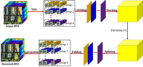
The mathematical symbols and explanations used in this paper are listed in

Table 1. The main mathematical symbols used in the paper and their corresponding explanations.

Natation	Description
x, x, X, $\mathcal{X}$	scalar, vector, matrix, tensor
xi	i-th entry of a vector x
xij	element (i, j) of a matrix X
${\mathcal{X}}_{ijk}$	the element in location (i, j, k) of a three-order tensor $\mathcal{X}$
$\Vert \mathcal{X}{\Vert }_F=\sqrt{{\displaystyle \sum }_{i_1=1}^{I_1}{\displaystyle \sum }_{i_2=1}^{I_2}\cdots {\displaystyle \sum }_{i_N=1}^{I_N}{x}_{i_1{i}_2\cdots i_N}^2}$	Frobenius norm of an N order tensor $\mathcal{X}\in {\mathbb{R}}^{I_1\times I_2\times \cdots \times I_N}$

. For further information on the tensor algebra, interested readers are referred to [28,29] for more details. For the three-order tensor $\mathcal{X}\in {\mathbb{R}}^{n_1\times n_2\times n_3}$, its block circulant matrix is defined as

$$bcirc\left(\mathcal{X}\right)=\left[\begin{array}{cccc}{\mathcal{X}}^{\left(1\right)}& {\mathcal{X}}^{\left(n_3\right)}& \cdots & {\mathcal{X}}^{\left(2\right)}\\ {\mathcal{X}}^{\left(2\right)}& {\mathcal{X}}^{\left(1\right)}& \cdots & {\mathcal{X}}^{\left(3\right)}\\ ⋮& ⋮& \ddots & ⋮\\ {\mathcal{X}}^{\left(n_3\right)}& {\mathcal{X}}^{\left(n_3-1\right)}& \cdots & {\mathcal{X}}^{\left(1\right)}\end{array}\right]$$

where ${\mathcal{X}}^{\left(k\right)}=\mathcal{X}\left(:,:,k\right)$ is the k-th front slice of $\mathcal{X}$.

3. Proposed Model

3.1. From WNNM to TWNNM

We consider the extension of NNM to WNNM as follows [19,20]

$${\min }_{\mathrm{X}}\Vert \mathrm{Y}-\mathrm{X}{\Vert }_F^2+\Vert \mathrm{X}{\Vert }_{\mathrm{w},\ast }$$

(1)

where $\Vert \mathrm{X}{\Vert }_{\mathrm{w},\ast }={\displaystyle \sum }_i{\mathrm{w}}_i{\sigma }_i\left(\mathrm{X}\right)$ represents the WNN of matrix X, $\mathrm{w}=\left[{\mathrm{w}}_1,{\mathrm{w}}_2,\cdots ,{\mathrm{w}}_n\right]$ (${\mathrm{w}}_i$ ≥ 0) denotes the weight vector, and ${\sigma }_i\left(\mathrm{X}\right)$ is the i-th singular value of matrix X. The Problem (1) has a closed-form solution of $\widehat{\mathrm{X}}={\mathrm{US}}_{\mathrm{w}/2}\left({\displaystyle \sum }\right){\mathrm{V}}^{\mathrm{T}}$, where Y = UΣV^T is the singular value decomposition (SVD) of matrix Y and ${\mathrm{S}}_{\mathrm{w}/2}(•)$ is a soft thresholding operator, which is defined as ${\mathrm{S}}_{\mathrm{w}/2}\left({{\displaystyle \sum }}_i\right)=max\left({{\displaystyle \sum }}_i-{\mathrm{w}}_i/2,0\right)$.

The HSI collected by optical imaging system are always contaminated by Gaussian noise [24]. The HSI data are a three dimensional cube, which can be denoted as a three-order tensor $\mathcal{X}=\left\{{\mathrm{X}}^1,{\mathrm{X}}^2,\cdots ,{\mathrm{X}}^b\right\}\in {\mathbb{R}}^{h\times v\times b}$, where each matrix ${\mathrm{X}}^i\in {\mathbb{R}}^{h\times v}\left(i=1,2,\cdots ,b\right)$ represents the i-th band of his; h and v represent the height and width in each band, respectively; and the HSI has b spectral bands. As our degradation model considers only Gaussian noise, the additive degradation model is

$$\mathcal{Y}=\mathcal{X}+\mathcal{N}$$

(2)

where $\mathcal{X},\mathcal{Y},\mathcal{N}\in {\mathbb{R}}^{h\times v\times b}$ denotes the underlying clean HSI, observed degraded his, and the Gaussian noise, respectively. According to our previous work [24], the tensor weighted nuclear norm minimization (TWNNM) model can be formulated as follows:

$$\frac{1}{2}\Vert \mathcal{Y}-\mathcal{X}{\Vert }_F^2+\Vert \mathcal{X}{\Vert }_{w,\ast }$$

(3)

3.2. Weighted Tensor Total Variation Regularization

Even though the method in the literature [24] can remove most of the noise, there is still room for improvement. As 2D total variation (TV) has been shown to preserve the local spatial piecewise smooth structure and suppress noise, it is widely applied to visual processing tasks [8,10]. HSI has a spatial dimension and spectral dimension. The clean spectral band should be smooth, so it is natural to use 3D weighted TV to preserve both the spatial and spectral smooth structure. It is defined as

$$\Vert \mathcal{X}{\Vert }_{3DWTV}={\lambda }_1\Vert D_h\mathcal{X}{\Vert }_1+{\lambda }_2\Vert D_v\mathcal{X}{\Vert }_1+{\lambda }_3\Vert D_p\mathcal{X}{\Vert }_1$$

(4)

where ${\lambda }_1$, ${\lambda }_2$, and ${\lambda }_3$ are three weight parameters, and $D_h$, $D_v$ and $D_p$ are the differential operators along the spatial horizontal direction, spatial vertical direction, and spectral direction, respectively. Based on the notations in Section 2, $D_h\mathcal{X}$, $D_v\mathcal{X}$, and $D_p\mathcal{X}$ at location (i, j, and k) are given by

$$\begin{gathered} D_h{\mathcal{X}}_{ijk}=\left|{\mathcal{X}}_{i+1,j,k}-{\mathcal{X}}_{ijk}\right|,D_v{\mathcal{X}}_{ijk}=\left|{\mathcal{X}}_{i,j+1,k}-{\mathcal{X}}_{ijk}\right|, \\ {D}_p{\mathcal{X}}_{ijk}=\left|{\mathcal{X}}_{i,j,k+1}-{\mathcal{X}}_{ijk}\right| \end{gathered}$$

(5)

3.3. Nonlocal Low-Rank Tensor Construction

When constructing the nonlocal low-rank tensor, we use the traditional nearest neighbor search (NNS). For an individual reference FBP with size m × m × b, we use NNS to find its k similar patches, Then, each FBP is unfolded into a matrix with size m² × 1 × b; all the k + 1 FBPs (including the reference one) are stacked into a three-order tensor with size m² × (k + 1) × b. This operation corresponds to the unfolding and stacking stages in Figure 1. Note that the constructed three order tensor jointly utilizes the spatial local sparsity, the non-local similarity in the spectral and spatial domains, and spectral high correlation. All of the FBPs denoised by the proposed TWNNM-TV are split into matrices with size m² × b; each matrix is folded as a FBP with size m × m × b, and all of the FBPs are aggregated into final denoised HSI. This operation corresponds to the splitting and folding stage in Figure 1.

To illustrate that the patch groups have a stronger low-rank property than the original HSI, we plot the first 40 singular values of the patch groups (blue curve) and the original patch (red curve) in Figure 2a. For a closer observation, we show the zoomed-in part of the singular value numbers between 10 and 20, as shown in Figure 2b. It can be seen from Figure 2a that the singular values of the patch groups are lower than those of the original HSI, and they decrease rapidly. This phenomenon demonstrates that the rank of the patch group is absolutely lower than that of the original HSI, and the same conclusion can be drawn from Figure 2b. Therefore, we apply the LR constraints on the patch group instead of on the original HSI.

3.4. Model Proposal and Optimization

Combined with the low-rank prior (TWNNM) and spatial–spectral smooth prior (TV) of the image component, the final optimization model for denoising HSI is as follows:

$$\frac{1}{2}\Vert \mathcal{Y}-\mathcal{X}{\Vert }_F^2+\Vert \mathcal{X}{\Vert }_{w,\ast }+{\lambda }_1\Vert D_h\mathcal{X}{\Vert }_1+{\lambda }_2\Vert D_v\mathcal{X}{\Vert }_1+{\lambda }_3\Vert D_p\mathcal{X}{\Vert }_1$$

(6)

The ADMM method [30] is used to solve the proposed model in Model (6). To this end, we introduce four auxiliary variables, $\mathcal{P}$, D₁, D₂, D₃ to Model (6), and it is equivalent to the following problem:

$$\begin{gathered} \frac{1}{2}\Vert \mathcal{Y}-\mathcal{X}{\Vert }_F^2+\Vert \mathcal{X}{\Vert }_{w,\ast }+{\lambda }_1\Vert D_h\mathcal{X}{\Vert }_1+{\lambda }_2\Vert D_v\mathcal{X}{\Vert }_1+{\lambda }_3\Vert D_p\mathcal{X}{\Vert }_1, \\ \mathrm{s}.\mathrm{t}.\mathcal{X}=\mathcal{P},D_1=D_h\mathcal{X},D_2=D_v\mathcal{X},D_3=D_p\mathcal{X} \end{gathered}$$

(7)

Problem (7) can be rewritten as its augmented Lagrangian form, as follows:

$$\begin{gathered} \mathcal{L}(\mathcal{X},\mathcal{P},D_1,D_2,D_3,{\mathsf{\Lambda }}_i)=\frac{1}{2}\Vert \mathcal{Y}-\mathcal{X}{\Vert }_F^2+\Vert \mathcal{P}{\Vert }_{w,\ast }+{\lambda }_1\Vert D_1{\Vert }_1+{\lambda }_2\Vert D_2{\Vert }_1+{\lambda }_3\Vert D_3{\Vert }_1 \\ +\frac{\mu }{2}(\Vert \mathcal{X}-\mathcal{P}+{\mathsf{\Lambda }}_1/\mu {\Vert }_F^2+\Vert D_1-D_h\mathcal{X}+{\mathsf{\Lambda }}_2/\mu {\Vert }_F^2+\Vert D_2-D_v\mathcal{X}+{\mathsf{\Lambda }}_3/\mu {\Vert }_F^2+ \\ \Vert D_3-D_p\mathcal{X}+{\mathsf{\Lambda }}_4/\mu {\Vert }_F^2) \end{gathered}$$

(8)

where ${\mathsf{\Lambda }}_i$ (i = 1, 2, 3, 4) are Lagrange multipliers, and μ represents the positive penalty parameter. For the multivariable optimization problem, the usual way is to fix other variables and optimize them alternately one by one. The optimization process is collected in Algorithm 1.

Algorithm 1 Optimization Process for Proposed Solver

1: Input: Noisy image $\mathcal{Y}$, regularization parameters λ1 = 1, λ2 = 1 and λ3 = 0.4, ε, kmax = 100, μmax = 106, ρ. 2: Initialize: Let $\mathcal{Y}$ = $\mathcal{X}$, D1 = D2 = D3 = 0, $\mathcal{P}$ = 0, k = 0, Λi = 0 (i = 1, 2, 3, 4) while not covered do 3: Update $\mathcal{P}$ via $\mathcal{P}=\mathrm{fold}\{S_{\nu ,\omega }(\mathcal{X}+{\mathsf{\Lambda }}_1/\mu )\}$ 4: Update D1 via $D_1=\mathrm{soft}(D_h\mathcal{X}+{\mathsf{\Lambda }}_2/\mu ,{\lambda }_1/\mu )$ 5: Update D2 via $D_2=\mathrm{soft}(D_v\mathcal{X}+{\mathsf{\Lambda }}_3/\mu ,{\lambda }_2/\mu )$ 6: Update D3 via $D_3=\mathrm{soft}(D_p\mathcal{X}+{\mathsf{\Lambda }}_4/\mu ,{\lambda }_3/\mu )$ 7: Compute $\mathcal{X}$ via FFT: $\mathcal{X}=\mathrm{ifftn}\left(\frac{\mathcal{C}}{\left(1+\mu \right)\mathbf{1}+\mu \mathcal{D}}\right)$ 8: Compute the Lagrange multipliers by ${\mathsf{\Lambda }}_1={\mathsf{\Lambda }}_1+\mu (\mathcal{X}-\mathcal{P}), {\mathsf{\Lambda }}_2={\mathsf{\Lambda }}_2+\mu (D_1-D_h\mathcal{X}), {\mathsf{\Lambda }}_3={\mathsf{\Lambda }}_3+\mu (D_2-D_v\mathcal{X}), {\mathsf{\Lambda }}_4={\mathsf{\Lambda }}_4+\mu (D_3-D_p\mathcal{X})$ 9: Update the penalty parameter $\mu =\min \{\rho \mu ,{\mu }_{\max }\}.$ 10: end while

Output: The restoration result $\mathcal{X}$.

By fixing the other variables, each of them can be optimized as following:

P1: ${\mathrm{argmin}}_{D_{1 }}{\lambda }_1\Vert D_1{\Vert }_1+\frac{\mu }{2}\Vert \mathcal{X}-\mathcal{P}+{\mathsf{\Lambda }}_1/\mu {\Vert }_F^2$

P2: ${\mathrm{argmin}}_{D_{2 }}{\lambda }_2\Vert D_2{\Vert }_1+\frac{\mu }{2}\Vert D_1-D_h\mathcal{X}+{\mathsf{\Lambda }}_2/\mu {\Vert }_F^2$

P3: ${\mathrm{argmin}}_{D_3} {\lambda }_3\Vert D_3{\Vert }_1+\frac{\mu }{2}\Vert D_2-D_v\mathcal{X}+{\mathsf{\Lambda }}_3/\mu {\Vert }_F^2$

P4: ${\mathrm{argmin}}_{\mathcal{P}} \Vert \mathcal{P}{\Vert }_{\mathsf{w},\ast }+\frac{\mu }{2}\Vert D_3-D_p\mathcal{X}+{\mathsf{\Lambda }}_4/\mu {\Vert }_F^2$

P5: $$\begin{gathered} {\mathrm{argmin}}_{\mathcal{X}} \frac{1}{2}\Vert \mathcal{Y}-\mathcal{X}{\Vert }_F^2+\frac{\mu }{2}(\Vert \mathcal{X}-\mathcal{P}+{\mathsf{\Lambda }}_1/\mu {\Vert }_F^2+\Vert D_1-D_h\mathcal{X}+{\mathsf{\Lambda }}_2/\mu {\Vert }_F^2 \\ +\Vert D_2-D_v\mathcal{X}+{\mathsf{\Lambda }}_3/\mu {\Vert }_F^2+\Vert D_3-D_p\mathcal{X}+{\mathsf{\Lambda }}_4/\mu {\Vert }_F^2) \end{gathered}$$

The subproblems P1, P2, and P3 are of the same form, and by using the soft-threshold shrinkage operator in the literature [31], they can be updated by

$$D_1=\mathrm{soft}(D_h\mathcal{X}+{\mathsf{\Lambda }}_2/\mu ,{\lambda }_1/\mu ), D_2=\mathrm{soft}(D_v\mathcal{X}+{\mathsf{\Lambda }}_3/\mu ,{\lambda }_2/\mu ), D_3=\mathrm{soft}(D_p\mathcal{X}+{\mathsf{\Lambda }}_4/\mu ,{\lambda }_3/\mu )$$

where $\mathrm{soft}\left(\mathrm{r},\mathsf{\theta }\right)=\mathrm{sign}\left(\mathrm{r}\right)\ast \max \left(\left|\mathrm{r}\right|-\mathsf{\theta },0\right)$.

The subproblem P5 can be solved by the following linear system:

$$\mho \mathcal{X}=\mathcal{Y}+\mu (\mathcal{P}-{\mathsf{\Lambda }}_1/\mu )+\mu (D_1+{\mathsf{\Lambda }}_2/\mu )+\mu (D_2+{\mathsf{\Lambda }}_3/\mu )+\mu (D_3+{\mathsf{\Lambda }}_4/\mu )$$

where $\mho \mathcal{X}=\left(1+\mu \right)ℐ+\mu \left(D_h^T{D}_h+D_v^T{D}_v+D_p^T{D}_p\right)$, and the $ℐ$ denotes unit tensor, $D_h^T$, $D_v^T$, and $D_p^T$ represent the transaction of $D_h$, $D_v$, and $D_p$, respectively. Here, it takes the periodic boundary condition for $\mathcal{X}$ into consideration, and the $\mathcal{X}$ in above linear system can be efficiently updated via 3D fast Fourier transform (FFT), as follows:

$$\mathcal{X}=\mathrm{ifftn}\left(\frac{\mathcal{C}}{\left(1+\mu \right)\mathbf{1}+\mu \mathcal{D}}\right)$$

where, $\mathcal{C}=\mathrm{fftn}(\mathcal{Y}+\mu (\mathcal{P}-{\mathsf{\Lambda }}_1/\mu )+\mu (D_1+{\mathsf{\Lambda }}_2/\mu )+\mu (D_2+{\mathsf{\Lambda }}_3/\mu )+\mu (D_3+{\mathsf{\Lambda }}_4/\mu ))$, $\mathcal{D}=D_h^T{D}_h+D_v^T{D}_v+D_p^T{D}_p$, fftn and ifftn represent the 3D FFT and its inverse operation, respectively.

For the subproblem P4, with Problem (1) in mind and according to the authors of [32], its closed-form solution is $\mathcal{P}=\mathrm{fold}\{S_{\nu ,\omega }(\mathcal{X}+{\mathsf{\Lambda }}_1/\mu )\}$, where $\nu =1/\mu$.

4. Experimental Results and Analysis

To evaluate our method for HSI denoising, we perform experiments on simulated and real-world data. The compared state-of-the-art denoising methods include the TV-regularized low-rank matrix factorization (LRTV) [8], the low-rank matrix recovery (LRMR) [18], the automatic hyperspectral image restoration (HyRes) [33], noise-adjusted iterative low-rank matrix approximation (NAILRMA) [34], and total variation regularized low-rank tensor decomposition (LRTDTV) [35]. The codes of these methods are downloaded from the authors’ homepages. For the parameters in the compared methods, they are manually adjusted to get the best results. For the weight parameters ${\lambda }_i$ (i = 1, 2, 3) in TV regularization, considering that ${\lambda }_1$ and ${\lambda }_2$ both control the spatial dimension of HSI, they should be assigned to the same weights. For simplicity, we set ${\lambda }_1$ = ${\lambda }_2$ = 1, and then we tune ${\lambda }_3$ according to reconstruction performance; it is found that the result is better when ${\lambda }_3$ = 0.4.

4.1. Experiment with Simulated Data

In the experiment with the simulated data, we add different intensity Gaussian noise to the Indian Pines dataset [36], whose size is 145 × 145 × 224.

(1) Visual effectiveness comparison: For visual comparison, the denoising results of different methods with the 11th band are presented in Figure 3 and Figure 4, and the corresponding variances of Gaussian noise are 20 and 60, respectively. It can be seen from Figure 3b and Figure 4b that the clean HSIs suffer degradation to a different degree. When the noise variance is 20, the compared methods could remove most of the Gaussian noise, but there is still obvious residual noise in LRMR and NAIRLMA. When the variance is 60, there is obvious residual noise in all of the compared methods. It can be observed from the enlarged yellow squares in the top left corner of Figure 3 and the top right corner of Figure 4 that the results obtained by our method preserve clearer and sharper edges, but the results obtained by HyRes and LRTV have blurred edges or an over-smooth phenomenon. In general, our method outperforms all of the compared methods at different noise levels.

(2) Quantitative comparison: Some frequently-used objective evaluation indexes are adopted, including the mean peak signal-to-noise ratio (MPSNR) [37], the mean structural similarity index (MSSIM) [37], the mean spectral angle mapper (MSAM) [38], and the Erreur Relative Globale Adimensionnelle de Synthese (ERGAS; relative dimensionless global error in synthesis in English) [39]. PSNR (its unit is dB) and SSIM are utilized to assess the similarity between the denoised image and the original image based on mean square error (MSE) and structural consistency, respectively. Larger values of MPSNR and MSSIM indicate that the results are better. ERGAS is used to measure the fidelity of the denoised image by calculating the weighted sums of the MSE of all the bands, while SAM denotes the average angle of spectrum vectors between the denoised HSI and its corresponding original image across all spatial positions. SAM fully reflects the spectral consistency of the denoised HSI with the original image. Smaller values of these two indexes represent better denoised results. The definitions of these indexes are as follows:

$$\mathrm{MPSNR}=\frac{1}{b}{{\displaystyle \sum }}_{i=1}^{b}10lo{g}_{10}\frac{{255}^2\times n_i}{\Vert {\widehat{u}}_i-u_i{\Vert }^2}$$

where b represents the number of spectral bands, and ${\widehat{u}}_i$ and $u_i$ are the restored image and the i-th band of the original clean image—they are of the same size. n_i represents the total number of pixels of image $u_i$.

$$\mathrm{SSIM}=\frac{\left(2{\mu }_x{\mu }_y+C_1\right)\left(2{\sigma }_{xy}+C_2\right)}{\left({\mu }_x^2+{\mu }_y^2+C_1\right)\left({\sigma }_x^2+{\sigma }_y^2+C_2\right)}, \mathrm{MSSIM}=\frac{1}{b}{{\displaystyle \sum }}_{i=1}^{b}SSI{M}_i$$

where ${\mu }_x$ and ${\mu }_y$ represent the average value of x and y images. ${\sigma }_x$ and ${\sigma }_y$ stand for the variance of x and y images, respectively, and ${\sigma }_{xy}$ is the covariance of these two images. C₁ and C₂ are constant here.

$$\mathrm{SAM}=\arccos \left[\frac{{{\displaystyle \sum }}_{i=1}^n{x}_i{y}_i}{\sqrt{{{\displaystyle \sum }}_{i=1}^n{x}_i^2}\sqrt{{{\displaystyle \sum }}_{i=1}^n{y}_i^2}}\right]$$

where S₁ = (x₁, x₂, …, x_n) and S₂ = (y₁, y₂, …, y_n) represent the spectral vectors at the same location in HSI.

$$\mathrm{ERGAS}=100\frac{h}{v}\sqrt{\frac{1}{b}{{\displaystyle \sum }}_{i=1}^b{\left(\frac{RMSE\left(x_i\right)}{\mu \left(i\right)}\right)}^2}$$

where h, v and b are defined above. RMSE (x_i) denotes the root-mean-square error (RMSE) for image x_i, and μ(i) denotes the mean of image y_i.

It is easy to see from

Table 2. Quantitative comparison of all of the compared methods under different noise variances for the Indian Pines dataset.

Variance	Index	Noisy	HyRes	LRTV	LRMR	NAIRLMA	LRTDTV	Proposed
	MPSNR	26.780	42.395	41.066	42.503	43.088	43.503	49.79
10	MSSIM	0.6566	0.9874	0.9958	0.9849	0.9845	0.9976	0.9987
	MSAM	0.0789	0.0116	0.108	0.0114	0.0104	0.0100	0.0038
	ERGAS	91.77	16.02	20.36	15.25	14.22	15.17	7.22
	MPSNR	20.763	37.469	38.815	36.522	38.214	41.092	43.330
	MSSIM	0.4366	0.9665	0.9927	0.9472	0.9586	0.990	0.9953
20	MSAM	0.1565	0.0200	0.0143	0.0227	0.0174	0.0136	0.0090
	ERGAS	183.45	28.26	25.82	30.412	25.22	19.32	14.891
	MPSNR	17.24	34.75	35.65	32.95	34.97	37.84	40.16
30	MSSIM	0.3240	0.9417	0.9863	0.8949	0.9219	0.9685	0.9902
	MSAM	0.2316	0.0270	0.0205	0.0343	0.0248	0.0204	0.0127
	ERGAS	275.15	38.30	33.94	46.10	36.15	27.44	20.48
	MPSNR	14.741	32.860	33.798	30.418	33.105	35.017	38.012
40	MSSIM	0.2528	0.9150	0.9787	0.8379	0.8933	0.931	0.9830
	MSAM	0.3037	0.0332	0.0252	0.0461	0.0299	0.0285	0.0157
	ERGAS	366.98	47.708	42.389	61.367	45.078	37.76	23.67
	MPSNR	12.80	31.44	32.10	28.51	31.22	32.76	35.78
	MSSIM	0.2031	0.8964	0.9697	0.7807	0.8524	0.8846	0.9734
50	MSAM	0.3719	0.0385	0.0309	0.0574	0.0367	0.0371	0.0212
	ERGAS	458.73	56.21	50.51	76.09	55.77	49.12	34.81
	MPSNR	11.219	30.279	30.898	26.981	29.723	30.821	34.983
60	MSSIM	0.1688	0.8687	0.9620	0.7259	0.8126	0.8339	0.9649
	MSAM	0.4359	0.0438	0.0360	0.0683	0.0432	0.0464	0.0228
	ERGAS	550.44	64.06	59.84	91.33	66.51	61.47	37.81
	MPSNR	9.88	29.24	29.71	25.61	28.58	29.26	32.70
70	MSSIM	0.1388	0.8488	0.9514	0.6745	0.7812	0.7806	0.9521
	MSAM	0.4964	0.0496	0.0428	0.0800	0.0485	0.0552	0.0321
	ERGAS	642.04	71.60	69.80	105.44	75.02	72.97	48.95
	MPSNR	8.717	28.459	28.787	24.572	27.582	27.939	32.202
80	MSSIM	0.1167	0.8262	0.9415	0.6297	0.7465	0.7314	0.9425
	MSAM	0.5523	0.0539	0.0472	0.0906	0.0544	0.0646	0.0333
	ERGAS	734.13	78.09	75.95	119.77	85.11	85.01	51.61
	MPSNR	7.70	27.72	27.68	23.52	26.61	26.71	31.62
90	MSSIM	0.0992	0.7981	0.9272	0.5856	0.7122	0.6806	0.9288
	MSAM	0.6044	0.0592	0.0584	0.1024	0.0606	0.0747	0.0354
	ERGAS	825.26	84.92	86.87	135.19	95.01	97.08	54.24
	MPSNR	6.78	27.10	26.60	22.62	25.71	25.72	31.13
100	MSSIM	0.0855	0.7827	0.9118	0.5463	0.6792	0.6396	0.9184
	MSAM	0.6528	0.0632	0.0665	0.1136	0.0668	0.0835	0.0362
	ERGAS	917.09	91.87	99.68	149.93	103.87	108.51	57.96

that the MPSNR values of our method are 3–7 dB higher than the maximum PSNR values of the compared methods. For MSSIM, the TV-regularization methods (LRTV, LRTDTV, and our method) achieve better results than the other methods, but the MSSIM values of our method are still higher than those of LRTV and LRTDTV. This indicates that the denoising results of our method have a better visual effect, and this is consistent with what we see in Figure 3 and Figure 4. To take a closer look at the SSIM and PSNR values of all the bands, we use noise variance 60 (see Figure 5) as an example. The results from Figure 5 show that our method outperforms almost all of the compared methods for each band, except that the SSIM values of our method in some bands are lower than those of LRTV.

On the account of nonlocal similarity, it can be seen from Table 2 that the MSAM and ERGAS values of our method are much lower than the other five methods. This can be interpreted as our method beng able to better maintain spectral information. To demonstrate the spectral fidelity achieved by our method, Figure 6 shows the spectral reflectance spectrum at location (55, 55) from all of the compared methods. In Figure 6, the blue curve represents the spectral reflectance values of the original image, and the orange curve represents the denoised spectral reflectance. It is not difficult to see that the spectral curve obtained by the proposed method achieves less spectral distortion and fits better to the original spectral curve than the compared methods.

4.2. Real-World Data Experiments

The performance on the simulated dataset is evaluated in Section 4.1. In this section, we choose two widely used real-world HSI datasets to verify the denoising performance. The first one is the Hyperspectral Digital Imagery Collection Experiment (HYDICE) urban dataset [40] and the second one is the Airborne Visible/Infrared Imaging Spectrometer (AVIRIS) Salinas dataset [36].

4.2.1. HYDICE Urban Dataset

The original dataset has 210 bands, and each band is a 307 pixel × 307 pixel grayscale image. In the experiment, we manually adjust the parameters of the compared methods accordingly to achieve the best results.

Figure 7 and Figure 8 display the denoising results of band 138 and band 206, respectively, with different methods. There is still plenty of residual noise in HyRes, LRMR, NAILRMA, and LRTDTV. For the LRTV, most noise is removed, but the result is over smooth. By considering the nonlocal low-rank property and spectral–spatial TV regularization, our proposed method shows superior performance on removing the Gaussian noise and preserving the spatial texture information and spectral information.

Based on the above analysis, we go further to evaluate all of the denoising algorithms with the mean cross-track profile (MCTP) [24]. All the MTCPs of 206th spectral band after denoising, along with the original MTCP, are presented in Figure 9. The horizontal axis and vertical axis in Figure 9 represent the column number and the mean digital number (MDN) values of each column, respectively. The existing noise leads to severe disturbances in the profile of the original image. After denoising, the disturbances are suppressed by the compared methods with different levels of success. In particular, the dead lines in Figure 7a are also eliminated, and the corresponding MTCPs are smoothed, as shown in the red circles in Figure 9. Evidently, our method provides a smoother mean profile, which is consistent with the results shown in Figure 7.

4.2.2. AVIRIS Salinas Dataset

This data contains 224 bands, and each band is a 512 × 217 pixel grayscale image. The original image is too large for display, so we extract a subimage of 300 × 217 pixels to show the denoising results. The second band in this dataset is contaminated by heavy Gaussian noise (Figure 10a), so we select this band to evaluate the denoising performance, the results are presented in Figure 10b–g. We can observe that the LRMR method completely failed to denoise this band. The HyRes and NAILRMA can remove some noise, but there is still obvious noise remaining. As for LRTV and LRTDTV, they have over-smoothed the image and distorted the structure, as presented in Figure 10c,f, and thus fail to give satisfactory results. Figure 10g indicates that the proposed method can still keep sharp edge when removing heavy noise. All of the curves of MDN with band 2 before and after denoising are presented in Figure 11. By comparison, our method achieves a better restoration result than the compared methods.

4.3. Discussion

(1) Parameters selection

The regularization parameters are discussed in Section 4.1. The other two parameters are related to the patch (size m × m × b), the parameters involved are m and k, and k is the number of similar patches in each cluster.

To determine the optimal values of m and k, the MPSNR index in the simulated experiments is used as the criterion. The curves of the MPSNR values with m under three different noise variance cases are shown in Figure 12a, in which the ${\sigma }^2$ represents noise variance. It can be seen that in the interval from 5 to 10, the MPSNR value increases with the increase of m. The most likely reason for this is that the damaged structure can be restored with the increase of m. As the value of m continues to increase, the MPSNR value gradually decreases, which indicates that under the optimal selection of m, a reasonably satisfactory denoising effect can be obtained. When the variance is 50, the MPSNR has a higher value when m = 11 than when m = 10. As the improvement is negligible, the patch size is set as m = 10 for all the experiments.

Moreover, the number of similar FBPs (k) is evaluated with the parameter m being fixed. The result in Figure 12b shows that the MPSNR index increases gradually until k = 40, thereafter it drops slowly. It can be explained that too many patches will destroy the low-rank property. Furthermore, more FBPs means a higher time cost, and we finally set the number of similar FBPs to 40.

(2) Convergence Analysis

To illustrate the convergence of the proposed method, the relative changes and MPSNR values versus the iteration number of our method are presented in Figure 13. It can be seen that the values of these two indexes tend to be stable after about 35 iterations, which clearly shows the convergence of our method.

(3) Operation time analysis

To test the computational complexity with compared algorithms, we select the running time of the Salinas dataset for comparison. The running times (in seconds) are shown in the

Table 3. Comparison of the running time.

Method	HyRes	LRMR	LRTV	NAIRLMA	LRTDTV	Proposed
Time (second)	29	0.209	483.42	439.21	942.92	587.08

. LRMR is the fastest, but its performances are the worst. Our algorithm is not the fastest, but also not the slowest.

5. Conclusions

To remove Gaussian noise, we propose a TV-regularization TWNNM model. In this model, we apply TWNNM on the HSI group clustered by NNS to characterize the LR property with similar patches. Moreover, TV regularization is utilized to not only suppress noise, but also keep the local smoothness in both the spatial and spectral domain. Experiments on both simulated and real HSI datasets indicate that our method can retain detailed information of the image better, while noise points are removed, which can be explained as by the fact that the combined LR and smooth prior information of the image component has the ability to accurately suppress noise and keep the smooth structure. Our method outperforms the state-of-the-art methods both in visual quality and evaluation criteria. Furthrmore, in further works, we will extend our method to other restoration tasks, such as magnetic resonance imaging (MRI) [41] and optical coherence tomography (OCT) images [42,43,44].

References

1. Shomorony, I.; Avestimehr, A.S. Is Gaussian noise the worst-case additive noise in wireless networks? In Proceedings of the 2012 IEEE International Symposium on Information Theory Proceedings (ISIT), Cambridge, MA, USA, 1–6 July 2012. [Google Scholar] [CrossRef]
2. Yang, J.; Zhao, Y.; Chan, J.C. Learning and Transferring Deep Joint Spectral–Spatial Features for Hyperspectral Classification. IEEE Trans. Geosci. Remote Sens. 2017, 55, 4729–4742. [Google Scholar] [CrossRef]
3. Yi, C.; Zhao, Y.Q.; Chan, J.C.W. Spectral super-resolution for multispectral image based on spectral improvement strategy and spatial preservation strategy. IEEE Trans. Geosci. Remote Sens. 2019. [Google Scholar] [CrossRef]
4. Bu, Y.; Zhao, Y.; Xue, J. Hyperspectral and Multispectral Image Fusion via Graph Laplacian-Guided Coupled Tensor Decomposition. IEEE Trans. Geosci. Remote Sens. 2020, 99, 1–15. [Google Scholar] [CrossRef]
5. Xue, J.; Zhao, Y.; Liao, W.; Chan, J.C.-W. Hyper-Laplacian Regularized Nonlocal Low-rank Matrix Recovery for Hyperspectral Image Compressive Sensing Reconstruction. Inf. Sci. 2019, 501, 406–420. [Google Scholar] [CrossRef]
6. Xue, J.; Zhao, Y.; Liao, W.; Chan, J.-W. Nonlocal Tensor Sparse Representation and Low-Rank Regularization for Hyperspectral Image Compressive Sensing Reconstruction. Remote Sens. 2019, 11, 193. [Google Scholar] [CrossRef] [Green Version]
7. Elad, M.; Aharon, M. Image denoising via sparse and redundant representations over learned dictionaries. IEEE Trans. Image Process. 2006, 15, 3736–3745. [Google Scholar] [CrossRef]
8. He, W.; Zhang, H.; Zhang, L.; Shen, H. Total-variation-regularized low-rank matrix factorization for hyperspectral image restoration. IEEE Trans. Geosci. Remote Sens. 2016, 54, 178–188. [Google Scholar] [CrossRef]
9. Othman, H.; Qian, S.-E. Noise reduction of hyperspectral imagery using hybrid spatial-spectral derivative-domain wavelet shrinkage. IEEE Trans. Geosci. Remote Sens. 2006, 44, 397–408. [Google Scholar] [CrossRef]
10. Yuan, Q.; Zhang, L.; Shen, H. Hyperspectral image denoising employing a spectral–spatial adaptive total variation model. IEEE Trans. Geosci. Remote Sens. 2012, 50, 3660–3677. [Google Scholar] [CrossRef]
11. Qian, Y.; Ye, M. Hyperspectral imagery restoration using nonlocal spectral-spatial structured sparse representation with noise estimation. IEEE J. Sel. Top. Appl. Earth Obs. Remote Sens. 2013, 6, 499–515. [Google Scholar] [CrossRef]
12. Wang, Y.; Niu, R.; Yu, X. Anisotropic diffusion for hyperspectral imagery enhancement. IEEE Sens. J. 2010, 10, 469–477. [Google Scholar] [CrossRef]
13. Wright, J.; Ganesh, A.; Rao, S.; Peng, Y.; Ma, Y. Robust Principal Component Analysis: Exact Recovery of Corrupted Low-Rank Matrices via Convex Optimization. In Proceedings of the Neural Information Processing Systems 2009, Vancouver, BC, Canada, 6–8 December 2009; pp. 2080–2088. [Google Scholar] [CrossRef]
14. Xue, J.; Zhao, Y.; Liao, W.; Chan, J.C.-W. Nonlocal Low-Rank Regularized Tensor Decomposition for Hyperspectral Image Denoising. IEEE Trans. Geosci. Remote Sens. 2019. [Google Scholar] [CrossRef]
15. Dong, W.; Shi, G.; Li, X. Nonlocal image restoration with bilateral variance estimation: A low-rank approach. IEEE Trans. Image Process. 2013, 22, 700–711. [Google Scholar] [CrossRef] [PubMed]
16. Xue, J.; Zhao, Y.; Liao, W.; Kong, S.G. Joint Spatial and Spectral Low-Rank Regularization for Hyperspectral Image Denoising. IEEE Trans. Geosci. Remote Sens. 2017, 99, 1–19. [Google Scholar] [CrossRef]
17. Zheng, Y.; Liu, G.; Sugimoto, S.; Yan, S.; Okutomi, M. Practical Low-Rank Matrix Approximation under Robust L1-Norm. In Proceedings of the 2012 Computer Vision and Pattern Recognition (CVPR), Providence, RI, USA, 16–21 June 2012; pp. 1410–1417. [Google Scholar] [CrossRef]
18. Zhang, H.; He, W.; Zhang, L.; Shen, H.; Yuan, Q. Hyperspectral image restoration using low-rank matrix recovery. IEEE Trans. Geosci. Remote Sens. 2013, 52, 4729–4743. [Google Scholar] [CrossRef]
19. Gu, S.; Zhang, L.; Zuo, W.; Feng, X. Weighted nuclear norm minimization with application to image denoising. In Proceedings of the IEEE Conference on Computer Vision and Pattern Recognition, Columbus, OH, USA, 23–28 June 2014; pp. 2862–2869. [Google Scholar] [CrossRef] [Green Version]
20. Gu, S.; Xie, Q.; Meng, D.; Zuo, W.; Feng, X.; Zhang, L. Weighted nuclear norm minimization and its applications to low level vision. Int. J. Comput. Vis. 2017, 121, 183–208. [Google Scholar] [CrossRef]
21. Cai, J.; Candes, E.J.; Shen, Z. A singular value thresholding algorithm for matrix completion. SIAM J. Optim. 2010, 20, 1956–1982. [Google Scholar] [CrossRef]
22. Wu, Z.; Wang, Q.; Wu, Z.; Shen, Y. Total Variation-Regularized Weighted Nuclear Norm Minimization for Hyperspectral Image Mixed Denoising. J. Electron. Imaging 2016, 25, 13037. [Google Scholar] [CrossRef]
23. Du, B.; Huang, Z.; Wang, N.; Zhang, Y.; Jia, X. Joint weighted nuclear norm and total variation regularization for hyperspectral image denoising. Int. J. Remote Sens. 2018, 39, 334–355. [Google Scholar] [CrossRef]
24. Kong, X.; Zhao, Y.; Xue, J.; Chan, J.-W. Hyperspectral Image Denoising Using Global Weighted Tensor Norm Minimum and Nonlocal Low-Rank Approximation. Remote Sens. 2019, 11, 2281. [Google Scholar] [CrossRef] [Green Version]
25. Wu, Z.; Wang, Q.; Jin, J.; Shen, Y. Structure tensor total variation regularized weighted nuclear norm minimization for hyperspectral image mixed denoising. Signal Process. 2017, 131, 202–219. [Google Scholar] [CrossRef]
26. Lefkimmiatis, S.; Roussos, A.; Maragos, P.; Unser, M. Structure tensor total variation. SIAM J. Imaging Sci. 2015, 8, 1090–1122. [Google Scholar] [CrossRef]
27. Berchtold, S.; Ertl, B.; Keim, D.A.; Kriegel, H.-P.; Seidl, T. Fast Nearest Neighbor Search in High-Dimensional Space. In Proceedings of the 14th International Conference on Data Engineering, Orlando, FL, USA, 23–27 February 1998; pp. 209–218. [Google Scholar] [CrossRef]
28. Kolda, T.G.; Bader, B.W. Tensor decompositions and applications. SIAM Rev. 2009, 51, 455–500. [Google Scholar] [CrossRef]
29. Xue, J.; Zhao, Y.; Liao, W.; Chan, J.C.; Kong, S.G. Enhanced Sparsity Prior Model for Low-Rank Tensor Completion. IEEE Trans. Neural Netw. Learn. Syst. 2019, 12, 1–15. [Google Scholar] [CrossRef] [PubMed]
30. Boyd, S.; Parikh, N.; Chu, E.; Peleato, B.; Eckstein, J. Distributed optimization and statistical learning via the alternating direction method of multipliers. Found. Trends Mach. Learn. 2011, 3, 1–122. [Google Scholar] [CrossRef]
31. Donoho, D.L. De-noising by soft-thresholding. IEEE Trans. Inf. Theory 1995, 41, 613–627. [Google Scholar] [CrossRef] [Green Version]
32. Zhang, C.; Hu, W.; Jin, T.; Mei, Z. Nonlocal image denoising via adaptive tensor nuclear norm minimization. Neural Comput. Appl. 2015. [Google Scholar] [CrossRef]
33. Rasti, B.; Ulfarsson, M.O.; Ghamisi, P. Automatic hyperspectral image restoration using sparse and low-rank modeling. IEEE Geosci. Remote Sens. Lett. 2017, 14, 2335–2339. [Google Scholar] [CrossRef] [Green Version]
34. He, W.; Zhang, H.; Zhang, L.; Shen, H. Hyperspectral Image Denoising via Noise-Adjusted Iterative Low-Rank Matrix Approximation. IEEE J. Sel. Top. Appl. Earth Obs. Remote Sens. 2015, 8, 3050–3061. [Google Scholar] [CrossRef]
35. Wang, Y.; Peng, J.; Zhao, Q.; Leung, Y.; Zhao, X.-L.; Meng, D. Hyperspectral image restoration via total variation regularized low-rank tensor decomposition. IEEE J. Sel. Top. Appl. Earth Obs. Remote Sens. 2017, 11, 1227–1243. [Google Scholar] [CrossRef] [Green Version]
36. Available online: http://www.ehu.eus/ccwintco/index.php?title=Hyperspectral_Remote_Sensing_Scenes (accessed on 11 May 2020).
37. Wang, Z.; Bovik, A.C.; Sheikh, H.R.; Simoncelli, E.P. Image quality assessment: From error visibility to structural similarity. IEEE Trans. Image Process. 2004, 13, 600–612. [Google Scholar] [CrossRef] [PubMed] [Green Version]
38. Yuhas, R.H.; Goetz, A.F.H.; Boardman, J.W. Discrimination among Semi-Arid Landscape Endmembers Using the Spectral Angle Mapper (SAM) Algorithm. In Proceedings of the 1992 Summaries of the 3rd Annual JPL Airborne Geoscience Workshop, Pasadena, CA, USA, 1–5 June 1992; JPL: Pasadena, CA, USA; pp. 147–149. [Google Scholar]
39. Kong, X.; Zhao, Y.; Xue, J.; Chan, J.-W.; Kong, S.G. Global and Local Tensor Sparse Approximation Models for Hyperspectral Image Destriping. Remote Sens. 2020, 12, 704. [Google Scholar] [CrossRef] [Green Version]
40. Available online: http://www.tec.army.mil/hypercube (accessed on 11 May 2020).
41. Yuan, J. MRI denoising via sparse tensors with reweighted regularization. Appl. Math. Model. 2019, 69, 552–562. [Google Scholar] [CrossRef]
42. Turani, Z.; Fatemizadeh, E.; Blumetti, T.; Daveluy, S.; Moraes, A.F.; Chen, W.; Mehregan, D.; Andersen, P.E.; Nasiriavanak, M. Optical Radiomic Signatures Derived from Optical Coherence Tomography Images to Improve Identification of Melanoma. Cancer Res. 2019, 79, 2021–2030. [Google Scholar] [CrossRef] [Green Version]
43. Adabi, S.; Rashedi, E.; Clayton, A.; Mohebbi-Kalkhoran, H.; Chen, X.-W.; Conforto, S.; Nasiriavanaki, M. Learnable despeckling framework for optical coherence tomography images. J. Biomed. Opt. 2018, 23, 1–12. [Google Scholar] [CrossRef] [Green Version]
44. Eybposh, M.H.; Turani, Z.; Mehregan, D.; Nasiriavanaki, M. Cluster-based filtering framework for speckle reduction in OCT images. Biomed. Opt. Express 2018, 9, 6359–6373. [Google Scholar] [CrossRef]
Figure 1. The flowchart of the proposed method.
Remotesensing 12 01956 g001
Figure 2. (a) Comparison of the low-rank property between the patch group and the original hyperspectral image (HSI). (b) Zoomed-in comparison of (a) when the singular number is between 10 and 20.
Remotesensing 12 01956 g002
Figure 3. Denoised results of the 11th band by different methods when the variance is 20: (a) original, (b) noisy, (c) HyRes, (d) total variation-regularized low-rank matrix factorization (LRTV), (e) low-rank matrix recovery (LRMR), (f) noise-adjusted iterative low-rank matrix approximation (NAILRMA), (g) total variation regularized low-rank tensor decomposition (LRTDTV), (h) and proposed.
Remotesensing 12 01956 g003
Figure 4. Denoised results of the 11th band by different methods when the variance is 60: (a) original, (b) noisy, (c) HyRes, (d) LRTV, (e) LRMR, (f) NAIRLMA, (g) LRTDTV, and (h) proposed.
Remotesensing 12 01956 g004
Figure 5. The peak signal-to-noise ratio (PSNR) value (a) and structural similarity index (SSIM) value (b) of each band when the noise variance is 60.
Remotesensing 12 01956 g005
Figure 6. Full band spectral reflectance curve at a spatial position (55, 55): (a) HyRes, (b) LRTV, (c) LRMR, (d) NAIRLMA, (e) LRTDTV, and (f) proposed.
Remotesensing 12 01956 g006
Figure 7. Denoised results by different methods of the 206th band in an urban dataset: (a) original, (b) HyRes, (c) LRTV, (d) LRMR, (e) NAILRMA, (f) LRTDTV, and (g) proposed.
Remotesensing 12 01956 g007
Figure 8. Denoised results by different methods of the 138th band in an urban dataset: (a) original, (b) HyRes, (c) LRTV, (d) LRMR, (e) NAILRMA, (f) LRTDTV, and (g) proposed.
Remotesensing 12 01956 g008
Figure 9. Vertical mean profiles of the denoising results of the 206 spectral band in the Hyperspectral Digital Imagery Collection Experiment (HYDICE) urban image: (a) original, (b) HyRes, (c) LRTV, (d) LRMR, (e) NAILRMA, (f)LRTDTV, and (g) proposed.
Remotesensing 12 01956 g009
Figure 10. Denoised results by different methods of the second band in the Salinas dataset: (a) original, (b) HyRes, (c) LRTV, (d) LRMR, (e) NAILRMA, (f) LRTDTV, and (g) proposed.
Remotesensing 12 01956 g010
Figure 11. Vertical mean profiles of the denoising results of the second spectral band in the Airborne Visible/Infrared Imaging Spectrometer (AVIRIS) Salinas image: (a) original band, (b) HyRes, (c) LRTV, (d) LRMR, (e) NAILRMA, (f) LRTDTV, and (g) proposed.
Remotesensing 12 01956 g011
Figure 12. PSNR value changes: (a) mean peak signal-to-noise ratio (MPSNR) versus patch size (m) and (b) MPSNR versus patch number (k).
Remotesensing 12 01956 g012
Figure 13. Convergence analysis with the iteration number: (a) relative changes X k + 1 X k F / X k F and (b) MPSNR versus the iteration number in the simulated Indian Pines dataset.
Remotesensing 12 01956 g013