The Implications of M3C2 Projection Diameter on 3D Semi-Automated Rockfall Extraction from Sequential Terrestrial Laser Scanning Point Clouds

Abstract

Rockfall inventories are essential to quantify a rockfall activity and characterize the hazard. Terrestrial laser scanning and advancements in processing algorithms have resulted in three-dimensional (3D) semi-automatic extraction of rockfall events, permitting detailed observations of evolving rock masses. Currently, multiscale model-to-model cloud comparison (M3C2) is the most widely used distance computation method used in the geosciences to evaluate 3D changing features, considering the time-sequential spatial information contained in point clouds. M3C2 operates by computing distances using points that are captured within a projected search cylinder, which is locally oriented. In this work, we evaluated the effect of M3C2 projection diameter on the extraction of 3D rockfalls and the resulting implications on rockfall volume and shape. Six rockfall inventories were developed for a highly active rock slope, each utilizing a different projection diameter which ranged from two to ten times the point spacing. The results indicate that the greatest amount of change is extracted using an M3C2 projection diameter equal to, or slightly larger than, the point spacing, depending on the variation in point spacing. When the M3C2 projection diameter becomes larger than the changing area on the rock slope, the change cannot be identified and extracted. Inventory summaries and illustrations depict the influence of spatial averaging on the semi-automated rockfall extraction, and suggestions are made for selecting the optimal projection diameter. Recommendations are made to improve the methods used to semi-automatically extract rockfall from sequential point clouds.

1. Introduction

1.1. Rockfall Hazard in Mountainous Terrain

Linear infrastructure systems which traverse rugged mountainous terrain can be exposed to various landslide hazards, including rockfall. Rockfall is characterized by fragment(s) of rock which detach from a cliff face and, subsequently, fall, bounce, and roll as the fragment(s) propagate downslope [1]. Although smaller in magnitude than other classes of landslides such as rockslides, rockfalls pose a significant threat to humans due to their intensity (kinetic energy) and their frequency, both temporally and spatially [2]. Rockfalls further challenge the safe operation of transportation corridors because it is difficult to prioritize the allocation of resources to be utilized to mitigate rockfall hazard across long transportation routes [3]. This task is particularly challenging in Canada, where there is over 45,000 km of rail track [4] which is susceptible to various geohazards. Rockfall hazard can be quantified along transportation corridors by conducting a rockfall hazard assessment [5]. As part of a quantitative hazard assessment, developing frequency-magnitude relationships from an inventory of events has become a common procedure [6]. These are power law relations; for rockfall, they are expressed as cumulative frequency-magnitude relationships. Cumulative frequency-magnitude relationships are derived by accessing inventories of known rockfall events, although spatial and temporal censoring of events can result in an inaccurate measurement of the hazard [3]. Censoring is caused by underreporting or inaccurate documentation of events, the lack of sufficient time to adequately capture high magnitude and low frequency events, or systematic censoring as a result of mitigation efforts obscuring or removing rockfall evidence [3]. Additional factors which can contribute to rockfall censoring include difficulties associated with observing rockfall source zones from infrastructure-level vantage points, heavy alteration of a rock mass preventing observation of fresh surfaces (an indicator of recent rockfall), and propagation of rockfall material well beyond the area of interest which, subsequently, eliminates evidence of a rockfall occurring.

1.2. Terrestrial Laser Scanning for Rockfall Monitoring

Terrestrial laser scanning (TLS) is a ground-based light detection and ranging (Lidar) method. Lidar is a remote sensing method used to acquire terrain information in the form of point clouds; a collection of data points in three-dimensional (3D) space. Lidar rapidly measures the reflected energy from an emitted laser [7,8], thus, acquiring detailed terrain point clouds with highly accurate measurements of the surface geometry. Over the last decade, TLS has become a routinely used data source for the characterization and monitoring of rock slopes, particularly, because the terrestrial platform is effective for capturing oblique views of vertical rock slopes [9]. TLS technology continues to advance, and as a result, practitioners have been able to capture data faster, at higher densities, and higher levels of accuracy [8]. Automated workflows have been developed to process these datasets, and therefore practitioners can spend more time analyzing and interpreting the data. Readers are referred to Lemmens [7] for a practical overview of TLS in the realm of remote sensing and geomatics, and to Telling et al. [8] for a review of the earth sciences research conducted with TLS.

With sequential datasets, practitioners can monitor active geomorphic processes occurring on rock slopes. Change detection between sequential TLS point clouds delineates rockfall source zones, from which volume is estimated and frequency-magnitude relationships can be derived [10]. A degree of automation has been added to the extraction of discrete rockfall events by utilizing clutter removal and density-based clustering algorithms [11]. Further improvements have been made in the accuracy of rockfall analysis, particularly for volume and shape calculations. Surface reconstruction algorithms have been used to construct 3D triangular meshes from rockfall point clouds, for estimating 3D volume [12,13,14]. There is, however, difficulty estimating 3D volumes because surface reconstruction algorithms are not always robust enough to consistently produce triangular meshes which are fully watertight (i.e., free of holes) and manifold (i.e., no overlapping facets and consistent normal orientation), while also effectively reconstructing and approximating the geometry of the object [15]. Bonneau et al. [16] showed that 3D computation of rockfall volume was highly sensitive to the surface reconstruction algorithm being utilized, and the authors provided recommendations for improved 3D rockfall volume calculations. Rockfall shape has also been quantified using 3D methods [17]. The shape of a rockfall is known to have a significant effect on its passage down the slope and its runout [18,19]. Detailed 3D rockfall shape has been carried forward into a new generation of rockfall models, which have incorporated custom rockfall objects and detailed terrain models [20,21,22].

Rockfall volume computation is commonly simplified using 2.5D raster methods [23,24]. While rasterized methods are robust, their output is highly sensitive to the selection of cell size and the affine transformation used to project the data onto the raster. Therefore, rockfall extraction and computation using the 2.5D method is, generally, less accurate as compared with the 3D method, as shown by Benjamin et al. [13].

1.3. Recent Developments for Rockfall Monitoring Using Laser Scanning

In addition to the research on rockfall extraction and analysis, recent studies have looked at upscaling monitoring programs with respect to spatial extents and data acquisition frequency. For the improvement of spatial extents, Benjamin [25] showed that a mobile laser scanning (MLS) system mounted onto a helicopter was capable of capturing detailed point clouds, and demonstrated the extraction of rockfall events along a 20 km length of coastal cliffs in England. A study of this size would not have been feasible using TLS. Furthermore, the helicopter mounted mobile platform resulted in an oblique view of the cliffs. Therefore, the system was capable of capturing topographic information on near vertical surfaces, which could not have been achieved with downward looking aerial laser scanning (ALS) surveys. Continuous terrestrial laser scanning systems have been investigated [26,27,28] for improving acquisition frequency. Williams et al. [24] established a workflow for automated rockfall extraction from hourly TLS datasets from an automated, fixed position TLS system. They found that increasing the time interval between data acquisitions resulted in a significant reduction in the number of small rockfall events captured [29]. The reduction in small magnitude events was due to the coalescence of multiple small rockfalls over the monitoring time interval [29]. However, there are limitations with regard to the spatial extent of the rock slopes that can be monitored with the use of fixed-position continuous TLS systems. Further research in (1) rockfall extraction methodologies, (2) systems for large extent data capture, and (3) frequent data capture or correction factors for infrequent data, would improve our ability to accurately measure rockfall hazard using laser scanning over large regions. This study focuses on the first research area outlined; improving rockfall extraction methodologies, specifically, through appropriate parameter selection in a commonly utilized change detection method.

1.4. Methods of Change Detection

Change detection between two datasets taken at different times can delineate active rockfall areas, from which information related to the rockfall events can be extracted and analyzed. There are several common change detection methods which have been used to capture surficial changes as a result of geomorphic processes, each with their respective advantages and disadvantages. These methods include the following: digital elevation model of difference (DoD), cloud-to-cloud (C2C), cloud-to-model (C2M), and multiscale model-to-model cloud comparison (M3C2).

Point clouds can be oriented and projected onto the x-y plane and rasterized into digital elevation models (DEMs). The subtraction of two DEMs produces a DEM of difference (DoD), which highlights change in one direction along the z-axis [30,31]. This method results in simple and fast computations, although for accuracy, it relies on the DEMs being capable of accurately modelling the terrain geometry; oriented terrain surfaces should be relatively orthogonal to the z-axis. An additional consideration is that DEMs cannot model overhanging features in the terrain, and the grid size can diminish the level of detail that can be captured from the DoD change detection [13]. Therefore, the DoD method is not very suitable for change detections on geometrically complex terrain with overhanging features and wide arrays of surface orientations. In order to improve the DoD accuracy across a challenging site, segments with similar orientations can be grouped together for separate analysis, although this can complicate processing and data interpretation [32].

Cloud-to-cloud (C2C) change detection computes the distance from each point in the second cloud to the closest point in the reference cloud [33]. Therefore, the direction along which the distance is computed is somewhat arbitrary, as it is based on whichever neighboring point is the closest. The measured C2C distance is sensitive to point spacing and surface roughness, and it is best suited for quickly computing distances between dense point clouds [32,33]. C2C distance computations do not provide directionally signed results [33,34], and therefore this method is less suitable for geomorphology studies where the ability to identify areas of loss and areas of deposition is desired [35].

Cloud-to-model (C2M) change detection computes the distance from each point in the second cloud to the closest point on a facet of a triangulated surface model of the reference cloud. Triangular facets allow interpolation between the reference point cloud, and thus result in distance calculation vectors which are less arbitrary as compared with the C2C method. Implementations of C2M have been used for semi-automated rockfall extraction [11,12,23], and for manual extraction using 3D software [36,37,38]. The accuracy of C2M depends on how well the surface mesh is able to model the terrain without over interpolating the original geometry of the input point cloud.

The multiscale model-to-model cloud comparison (M3C2) algorithm created by Lague et al. [34] measures the distance along a local normal vector estimated from each point’s neighborhood, and thus considers local surface orientation in the distance computations. The algorithm projects search cylinders along the local normal vectors to find the locally averaged change between the two clouds. The M3C2 algorithm operates directly on the point clouds, and therefore requires no meshing or gridding, which can induce geometry errors in the terrain model as noted earlier. As a result, M3C2 has become a widely used and preferred method for change detection in various fields, including the monitoring of rock slopes and cliffs with TLS [13,14,24,25,26,29,39], landslide deformation [27], retrogressive thaw slump monitoring [32], rockfall model calibration [22], archaeological monitoring and preservation [40,41], structure from motion (SfM) photogrammetry monitoring and error analysis [42,43,44], and various other monitoring applications in the geosciences [35,45,46,47]. The M3C2 method is also widely used because it is freely available as a plugin within the open-source software CloudCompare [48]. Direct operations on the point cloud and locally oriented distance computations make the M3C2 algorithm ideal for identifying change on structured rock masses with laser scanning data. Because it is a commonly used change detection method, M3C2 was chosen to be the focus of this study as we evaluated the influence of a key M3C2 parameter on the outcome of semi-automated rockfall extraction from sequential TLS datasets. An explanation of the M3C2 algorithm and its input parameters is provided in the following section.

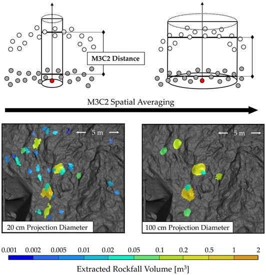
1.5. Multiscale Model-to-Model Cloud Comparison (M3C2)

The M3C2 algorithm calculates a local average cloud-to-cloud distance for a point in the reference cloud, termed the core point, through the use of a search cylinder projected along a locally oriented normal vector (Figure 1) [34]. Then, the distance is assigned as an attribute of the core point.

The entire reference cloud can be defined as core points, or a subsampled set of the reference cloud. The original resolution of both point clouds is used in the M3C2 computations regardless of whether the data is subsampled in the process. The core point’s normal vector is estimated from its surrounding neighborhood, which should be of a scale such that it captures the surface geometry without being sensitive to local surface roughness [34]. Points encompassed by the search cylinder are used to compute the average position of Cloud 1 and Cloud 2. The distance between the average positions (along the normal vector) is the M3C2 distance (Figure 1). The search cylinder geometry is defined by the user, which controls the degree of spatial averaging that occurs, as shown in Figure 1, where two different projection diameter sizes are depicted. If there are no Cloud 2 points captured within the cylinder, no distance is computed. The projection diameter size is chosen based on the application, point spacing, and surface complexity [34]. Readers are referred to Lague et al. [34] for further details on the M3C2 algorithm.

1.6. Study Objectives

Although there has been much research utilizing M3C2 to monitor and extract changes in terrain, there is little guidance on the optimal parameters to be used. Furthermore, there is a lack of reporting of the M3C2 parameters used in various studies. M3C2 parameters should be chosen as a function of the type and magnitude of the process that is being investigated, the density of data, and the complexity of the terrain [34]. This study aims to help users select appropriate M3C2 parameters for effective extraction of rockfall. The impact of the M3C2 projection diameter on semi-automated rockfall inventory results is investigated. Included in this study are the following:

• An overview of a five-year TLS monitoring campaign for an active rock slope along the Fraser River, in the interior of British Columbia, Canada;
• The full presentation of the semi-automated workflow used in this work for extracting rockfall and computing 3D volume and shape;
• The creation of six different rockfall inventories using different M3C2 projection diameters ranging from two times the average point spacing to ten times the average point spacing;
• An analysis of the impact that the M3C2 projection diameter has on automated rockfall extraction;
• A discussion on the considerations that should be made when selecting appropriate M3C2 parameters for future work;
• Recommendations for improvements on automated rockfall extraction.

1.7. Study Site

The study site, Canadian National (CN) Ashcroft Mile 109.4, is a rock slope located along the Fraser River in the interior of British Columbia (BC), Canada, approximately 150 km northeast of Vancouver, BC. The study site spans roughly 250 m of the CN track, which traverses the base of the slope (Figure 2). The Trans-Canada Highway lies above the top of the rock slope.

The slope morphology largely consists of exposed bedrock with areas of talus, scattered vegetation, and an overlying layer of soil on the upper reach of the slope. The bedrock is part of the Jackass Mountain Group, a thick succession of Cretaceous shallow-water deltaic sedimentary rock [49], with bedding that dips at moderate angles into the slope [50]. The slope is comprised of the following five units: a highly fractured greyish brown argillite, a sandy siltstone, a thin black shale layer, a sandstone, and a thick bedded pebble conglomerate. The five units and a bedrock geology model are presented in Figure 3. The mean slope angle ranges from 45 to 55° [51]. There are four major joint sets which contribute to sliding, wedge, and toppling failures [50,51] plotted in Figure 4.

Mile 109.4 has been of particular interest due to the high activity of slope movements, most notably a 53,000 m³ rockslide occurring in November 2012 (Figure 5a,b). The rockslide was bounded by two local faults which crosscut the slope [50]. The rockslide covered the track with more than 15 m³ of debris and destroyed the pre-existing rock shed [52]. An 80 m long rock shed was designed and completed in the fall of 2014. The design allows for a talus cone to build on top of the structure, which then guides future failures over top of the track (Figure 5c,d). For more information on the geological units and the 2012 rockslide, readers are referred to Sturzenegger et al. [50].

2. Materials and Methods

2.1. Data Collection

2.1.1. Terrestrial Laser Scanning

Terrestrial laser scanning was conducted at CN Ashcroft Mile 109.4 at weekly to seasonal intervals from November 2013 to December 2018. The survey consisted of a singular scan position approximately 400 m from the study slope across the Fraser River, on a soil slope above the CP track (Figure 2 and Figure 6). Additional scan positions with a suitable viewpoint of the slope were not possible due to site accessibility and obstruction by dense vegetation. Two time-of-flight TLS systems were used to collect data at the site throughout the 5-year monitoring period. A timeline of the TLS data acquisitions is outlined in Figure 6.

Monitoring began in November of 2013 using an Optech Ilris 3D time-of-flight system (Figure 6a). The Optech Ilris 3D system has a manufacturer-specified accuracy of 7 mm in range, and 8 mm in vertical and horizontal directions from a distance of 100 m [53]. The maximum range at 20% target reflectivity is approximately 800 m [54]. A total of 23 scans were taken from November 2013 to late August 2017 with the Optech system. Monitoring with the Riegl VZ-400i time-of-flight system (Figure 6b) commenced in early September 2017. Laser scanning hardware influences the error in the spatial terrain information captured; the wavelength the systems are operating at, the precision and accuracy of the systems, beam divergence at range, the minimum angular increment both in vertical and horizontal, the maximum range at select target reflectivity, in addition to the environmental sensitivities of the systems [55]. Therefore, a separate Riegl baseline scan was taken after the last Optech scan, to avoid comparing datasets from different scanners. The Riegl VZ-400i scanner has a manufacturer-specified accuracy of 5 mm and precision of 3 mm from a distance of 100 m [56]. The maximum range with a 100 Hz pulse rate and 20% target reflectivity is approximately 400 m [56]. A total of 8 scans were taken with the Riegl system from early September 2017 to December 2018. Figure 6c shows the total number of days on which various portions of the slope were monitored. The extents of the scan area generally increased over time. Additional variations were due to the fact that the scan extents were uniquely defined during each site visit by different personnel.

With each TLS scan, the associated intensity of the reflected laser pulse was dependent on surface characteristics (color, roughness, and moisture), the beam wavelength, and the presence of atmospheric particles such as dust and water [9,55], as well as ash and smoke from forest fires. Conducting TLS surveys when there was no moisture on the slope was not possible through late fall and winter months due to higher amounts of precipitation in the region. As a result, scans taken during less optimal weather conditions have poor returns and holes in the data. A total of 4 scanning dates were omitted from the study in order to optimize the spatial resolution of datasets without overly increasing the time intervals between scans.

Optech Ilris scans were parsed using Optech Parsing software. Vegetation and non-stable infrastructure (i.e., slide detector fences and metal mesh installed on the slope surface) were manually removed from the raw point clouds using the Polyworks PIFEdit module [57]. Then, the cleaned point clouds were aligned to the November 2013 baseline using the Polyworks IMAlign module [57]. First, a coarse alignment was performed by manual point picking of stable areas of the slope with sharp identifiable geometry, such as stable bedrock and infrastructure. The coarse alignment was followed by a fine alignment process using Polyworks’ iterative surface matching based on the iterative closest point (ICP) algorithm [58]. Areas of significant known change were manually removed from the fine alignment process to improve the quality of alignment [52]. The Riegl VZ-400i scans were processed in a similar fashion solely using the RiScan Pro software package [59]. Coarse and ICP fine alignment was conducted to align the scans to the September 2017 baseline. The registration error for all the datasets varied between 1 and 2 cm. The point spacing typically ranged between 3 cm and 10 cm across the site for all datasets.

2.1.2. High-Resolution Panoramic Photography

High-resolution panoramic photos were generated from a series of photos captured during each field campaign to aid in the interpretation of TLS data. High-resolution photographs were taken from the scan position (Figure 2 and Figure 6) using a 36 megapixel Nikon D800 full frame (November 2013 to September 2017) and a Nikon 24 megapixel D7200 cropped (September 2017 to December 2018) DSLR camera, both equipped with a Nikkor 135 mm f/2.0 prime lens. The camera was mounted onto a Gigapan Epic Pro motorized panoramic head [60]. The photos were stitched together using the GigaPan Stitch software, resulting in a seamless high-resolution panoramic photo of the rock slope.

2.1.3. Oblique Helicopter Photogrammetry

An oblique aerial photogrammetry survey from helicopter (OAP-H) was conducted in December 2014 after two 200 m³ rockfall events and a 3300 m³ event [51]. Photos were captured using a Nikon D800 full-frame DSLR camera equipped with a Nikkor 50 mm prime lens. Structure-from-motion multi-view-stereo (SfM-MVS) photogrammetry was used to build a model from 162 photos using the Agisoft PhotoScan Professional V.1.3.2 software package [61]. The point cloud was built using a typical SfM-MVS workflow [62,63]. The point cloud was aligned and scaled to the September 2017 Riegl TLS baseline using point picking coarse alignment and ICP fine alignment within CloudCompare [48], resulting in a root mean square error of approximately 3.3 cm. To improve the results, areas of significant known change were excluded from the alignment procedure.

2.2. Rockfall Extraction and Database Aggregation

The rockfall extraction process is depicted in Figure 7. Change detection was conducted to outline active areas of change due to rockfall. Change forward in time (A to B) highlights the back surfaces of areas of loss. Change backwards in time (B to A) highlights the fronts of changing features. A limit of detection threshold was used to extract the fronts and backs of loss features. The extracted features were merged to create an unorganized point cloud of loss objects. Clutter and change detection artifacts were manually removed from the point cloud. Clutter was generated as a result of random noise within the TLS datasets and change detection. Artifacts were generated as a result of systematic errors within the M3C2 change detection algorithm, mainly edge effects near occlusions and noise caused by the search cylinder passing through multiple separate surfaces [24]. Objects attributed to talus, soil, and vegetation movements were also manually removed, resulting in an unorganized point cloud of solely rockfall objects. Density-based clustering was used to give a unique ID to each of the rockfall objects, and to remove any remaining noise left over. For each object, 3D volume and shape were computed, and the lithology was classified by comparing the rockfall centroids to a mapped 3D geological model of the site. Lastly, false positive rockfalls were filtered out using: (1) a ratio threshold of positive to negative points and (2) a lowest volume threshold [14]. These steps were conducted for each sequential TLS dataset, resulting in 25 clustered rockfall datasets, each containing the extracted rockfall events with the numerous computed attributes. Further details of the rockfall extraction workflow are explained in the following subsections.

2.2.1. M3C2 Batch Change Detection

M3C2 change detection was conducted for all 26 sequential TLS datasets using a Python batching script to access the command line API of CloudCompare. An intermediate affine transformation was applied to the TLS datasets prior to the M3C2 distance computation to align the point clouds with a Cartesian axis, which ensures the correct orientation of normal vectors. Core points were defined at a subsampled point spacing of 10 cm, representing the maximum point spacing across the datasets. Subsampling normalized the point spacing across the study site and was important for the use of a density-based clustering algorithm in a later step of the workflow. The full resolution of the clouds was used for the normal vector estimation and distance computations, even though the data was subsampled. The projection diameter was varied at the following six different multiples of the point spacing: 20, 30, 40, 50, 75, and 100 cm. The projection length was fixed at 15 m for all computations. In order to ensure that the normal vector orientation is not affected by roughness, it has been recommended that the normal search diameter, D, is at least 20–25 times larger than the roughness computed at the equivalent scale [34]. The normal search diameter was fixed at 1 m, which was approximately 30 times the average surface roughness.

2.2.2. Extraction of 3D Loss Objects

M3C2 calculations were conducted for all sequential datasets, forward in time. Negative change areas corresponded to rockfall back scarps and areas of talus or soil depletion. Significant negative change was extracted using a consistent 5 cm limit of detection at 95% confidence (LoD₉₅), representing two times the maximum root mean square error determined during the point cloud alignment procedure. Then, M3C2 calculations were conducted for all sequential datasets, backward in time. Similarly, positive change extracted using the LoD₉₅ delineated the fronts of rockfalls, talus, or soil movements. For each pair of sequential datasets, the extracted negative and positive change were merged together, resulting in a point cloud of 3D loss objects yet to be clustered. Clutter and artifact points could remain in the loss object cloud, as a result of their M3C2 distances being larger than the LoD₉₅.

2.2.3. Classification of Rockfall and Removal of Clutter and Artifacts

Objects that were not the result of rockfalls had to be removed, such as remaining low-lying vegetation, talus, and soil. The classification of points corresponding to rockfall can be automated by comparing extracted objects to a 3D classified mask, as demonstrated by Bonneau et al. [17]. Work has been undertaken to start automatically classifying point clouds into areas of vegetation, soil, talus, and bedrock [64], although in complex terrain such as at Mile 109.4, automated classification methods may not be sufficiently robust to have complete confidence in the resulting mapping. Additionally, the study site has undergone significant natural and engineered slope changes throughout the period of the monitoring program (Figure 5). A singular bedrock classification mask would likely not suffice for accurate automated rockfall classification. Therefore, this step was done manually to maximize the accuracy of classification, and to prevent the omittance of events or inclusion of false positives as a result of potential systematic error within an automated workflow.

Points not attributed to rockfall were removed in CloudCompare using the snipping tool. Gigapixel panoramic photos taken with each data acquisition were used to identify loss features that were located in areas of talus, soil, and vegetation. Additional tools within CloudCompare were used to aid in classifying the change signatures. These tools included the visualization of normal vectors and slope angle in an underlying terrain model, and the visualization of accumulation areas in previous change detection time intervals. For a singular change detection time interval, the point clouds corresponding to all six projection diameters were processed simultaneously to ensure the equal treatment of each dataset.

Remaining clutter and artifacts were removed in parallel with the rockfall classification. This included edge effects near the borders of occluded data (areas not in the line of sight of the scanner), noise as a result of high scanner incidence angles and positional uncertainty, and noise generated by the M3C2 projection cylinder contacting multiple surfaces [24]. This process was a much simpler task as compared with rockfall classification, as these points were apparent with strong linear features or noisy sporadic magnitudes of change, with little to no defined geometry.

2.2.4. Clustering Individual Rockfalls

As discussed by Tonini and Abellan [11], an adaptation of the density-based spatial clustering of applications with noise (DBSCAN) algorithm [65] was used to cluster individual rockfall events from the unorganized input point cloud. The DBSCAN algorithm is depicted in Figure 8. The clustering algorithm uses a search radius and a minimum number of points to define a cluster. These two parameters were tested in a trial and error process using datasets of varying difficulty, and the results were visualized in CloudCompare. Similar to the findings by van Veen et al. [14], it was determined that the DBSCAN algorithm performed optimally when using a minimum of 12 points and a 30 cm search radius. The DBSCAN algorithm was implemented in C++. The clustering process resulted in a point cloud of grouped rockfall objects, each with a unique ID.

2.2.5. Volume Calculations

Surface reconstruction was used to compute the volume of each rockfall 3D object extracted. This study used the alpha-shape algorithm developed by Edelsbrunner and Mücke [66]. An alpha shape is a generalization of the convex hull of a point set. An alpha shape is defined as the union of all simplices covered by its alpha complex, where the alpha complex comprises all Delaunay tetrahedra (and encompassing faces, edges, points) which have empty circumspheres, with radii less than the defined alpha radius. Therefore, for a set of points, there exists a family of alpha shapes, with each member corresponding to a different value of alpha radius, ranging from zero to infinity. An infinite alpha radius produces the convex hull of the set of points, and thus simplifies the geometry. An alpha radius of zero results in solely the set of points, with no edges or faces defined, thus, having no geometry. Therefore, an optimal alpha radius is required to best approximate the geometry of the object. Readers are referred to Edelsbrunner and Mücke [66] for further details and discussions of alpha shapes.

As mentioned earlier, the triangulated mesh resulting from surface reconstruction needs to be manifold and fully watertight in order to ensure the accuracy and reliability of volume calculations. The alpha-shape approach does not guarantee either of these characteristics. Therefore, the iterative alpha-shape approach, by Bonneau et al. [16], was implemented to guarantee that all resulting alpha shapes were fully watertight and manifold. This was performed by iterating through each member of the alpha shape family and finding the lowest alpha radius which satisfied the aforementioned criteria. A lower alpha radius also results in a better approximation of the surface geometry of the rockfall object, as well as a better estimation of volume. The iterative alpha shape surface reconstruction was implemented in MATLAB [67].

2.2.6. Shape Calculation

The shape of a rockfall can provide insight into the structure of the sourcing rock and the failure mechanics. With a new generation of 3D rockfall modeling software, the shape of a rockfall and the quality of the rock can also give insight into its chaotic interaction with terrain and the potential runout of the fragment(s) [20,21,22]. Blott and Pye [68] described shape using four important characteristics; form, roundness, irregularity, and sphericity. The quantification of form involved the measurement of the length, breadth, and thickness of a particle, typically with all measurements being mutually orthogonal [68]. In 1958, Sneed and Folk [69] proposed a ternary diagram to classify the form of pebbles into 10 categories, as relations among the longest (A), intermediate (B), and shortest (C) axes. This study, in addition to several other studies [14,25,28], used the Sneed and Folk classifications to classify the shape of 3D rockfalls extracted from TLS. The Sneed and Folk ternary diagram and classifications are shown in Figure 9.

The rockfall shape was computed using the adjusted bounding box algorithm from Bonneau et al. [17]. The rockfall point cloud is rotated to align the direction of maximum variance with the x-axis in Cartesian space, and its axes are computed using a bounding box. In contrast to a regular bounding box approach, this method guarantees that the A-axis is the longest dimension of the object [17].

2.2.7. Lithology Classification

The extracted rockfalls were also classified into different lithologies by comparing the source area to a geological model. Due to logistical and safety constraints, field mapping of the study slope was not possible. Therefore, a 3D geological model was created by visually mapping the OAP-H point cloud in Agisoft PhotoScan into the five lithology classes defined previously (Figure 3). Various visual aids, in addition to the colored 3D point cloud, were used to improve the geological interpretation. These included the use of gigapixel panoramic photos where lithological features were prominent, and reference to the geological interpretation and field mapping conducted as part of the study by Sturzenegger et al. [50]. Each rockfall object centroid was computed and compared to the geological model [17]. A vote was conducted using nine nearest neighboring points to give each rockfall a hard classification of lithology.

2.2.8. Filtering

The last step in the rockfall extraction process was filtering and removal of false positive rockfall events. First, the rockfalls were filtered based on the ratio of positive to negative points (M3C2 distance), to ensure all rockfall clusters were 3D objects with fronts and backs. A minimum ratio of 1:3 was selected [14]. Secondly, volume filtering was conducted to remove rockfalls which were, theoretically, too small to be extracted given the workflow and data density. A minimum volume of 0.001 m³ was defined, suggesting a 12-point rectangular prism with dimensions 30 by 10 by 5 cm, corresponding to the 10 cm point spacing, 5 cm limit of detection, and 12-point minimum cluster size used in the DBSCAN algorithm.

3. Results

A total of six rockfall inventories were created for the 20, 30, 40, 50, 75, and 100 cm M3C2 projection diameters. All inventories contained 25 scan intervals, although in two intervals no rockfall activity was identified. The centroids of each rockfall in the 20 cm projection diameter inventory are plotted in Figure 10, with their date range of occurrence and volume discretized.

Table 1. The number of rockfalls extracted and filtered for each inventory with differing M3C2 projection diameters.

Number of Rockfalls	20 cm	30 cm	40 cm	50 cm	75 cm	100 cm
Conglomerate	12	11	11	10	8	5
Sandstone	923	866	804	689	487	308
Shale	897	820	750	639	455	290
Sandy siltstone	1547	1436	1287	1124	815	531
Argillite	262	247	230	200	147	95
Total filtered	14	16	10	11	9	7
Grand total	3641	3380	3082	2662	1912	1229

summarizes the number of rockfall events extracted in each inventory and

Table 2. Rockfall volume properties of each inventory with differing M3C2 projection diameters.

Rockfall Volume [m3]	20 cm	30 cm	40 cm	50 cm	75 cm	100 cm
Minimum	1.01 × 10−3	1.02 × 10−3	1.03 × 10−3	1.25 × 10−3	1.11 × 10−3	1.43 × 10−3
Maximum	3850	3852	3856	3859	3913	3862
Median	1.19 × 10−2	1.27 × 10−2	1.50 × 10−2	1.92 × 10−2	3.64 × 10−2	7.39 × 10−2
Average	1.63	1.76	1.96	2.28	3.30	5.19
Total	5944	6002	6113	6186	6443	6582

summarizes the rockfall volume properties for each inventory. The study site has been fairly active over the five years of monitoring, likely due to the major slope changes that occurred prior to the beginning of the monitoring campaign. There is a significant variation in the number of rockfalls in each of the inventories. As the projection diameter increases, the total number of extracted rockfall events decreases. This decrease is attributed to a higher degree of spatial averaging occurring with larger projection diameters, which makes smaller changing features less prominent, and therefore less likely to be clustered into individual rockfall events.

Table 2 demonstrates the calculated volume of the rockfall events, depending upon the projection diameter. Increased projection diameters cause the minimum, median, and average rockfall volumes to increase. The cumulative rockfall volume also increases as the projection diameter increases, and therefore is controlled by the uncertainties on larger rockfall events, rather than the omittance of many low magnitude rockfall events. The increase in uncertainty is likely due to spatial averaging resulting in the extraction of points which are not part of the rockfall area. Extraction of additional points expands the convex hull of the object, and therefore expands the domain of the alpha shape, and its volume. Interpolation error following the iterative alpha-shape surface reconstruction can result in a higher volume captured [16], shown by the volume of the largest event increasing as the projection diameter increases (Table 2). Interestingly, the maximum rockfall magnitude begins to decrease between the 75 and 100 cm inventories, suggesting that each rockfall has a projection diameter which maximizes its boundary and volume estimate. Beyond the volume-maximizing projection diameter, the degree of spatial averaging begins to reduce the object’s convex hull, therefore, reducing the boundary of its alpha shape and subsequent volume.

Another consideration is the production of larger magnitude rockfalls by the coalescence of multiple smaller rockfalls, as a result of spatial averaging in M3C2. This would be possible through the intermediate points separating multiple rockfalls in close proximity, if their calculated M3C2 distances exceed the LoD₉₅ due to spatial averaging. The intermediate points would be extracted and allow for the multiple density-based clusters to be connected across them. The trends interpreted and discussed from Table 1 and Table 2 are further illustrated in Figure 11, where the volumetric distributions of rockfall for each inventory are shown.

An increase in the projection diameter significantly reduces the number of lower magnitude rockfalls that are extracted, specifically in the range of 10⁻³ to 4 × 10⁻¹ m³, shown by the downward shift in the early portion of the cumulative frequency-magnitude relationships in Figure 12. The linear portions of all the cumulative frequency-magnitude relationships are similar for the tested projection diameters. The relative deviations in volume are higher at the magnitudes of 5 to 400 m³, causing the cumulative frequency-magnitude curves to diverge. The curves converge again at the largest magnitude event recorded, where there is less relative deviation in volume.

Figure 13 and Figure 14 show the reduction of lower magnitude rockfall events, spatially, at select areas of the study site. As the M3C2 projection diameter increases, the smaller rockfalls are not captured in the inventories. Remaining rockfalls begin to lose their defined shape as the change detection signature can appear ”blurred” as a result of the spatial averaging. In special cases of multiple discrete rockfall events in close proximity to one another, the blurring of the change detection signature causes events to be coalesced into one clustered rockfall.

The shift in the change detection signatures resulting from increasing the spatial averaging is further reflected in the shape of the extracted rockfall events. The shape of each rockfall was computed using the adjusted bounding box approach discussed in the Methods section. Two distinctly different lithologies, the shale and the sandy siltstone, were analyzed to see how the M3C2 projection diameter influences the shapes of the rockfall events. The average shape for (a) the sandy siltstone rockfalls and (b) the black shale rockfalls is plotted in Figure 15. The average rockfall shape for both the sandy siltstone and the shale tended to be bladed, with the shale being slightly more bladed. It is noted that the average shape of rockfall, ranging from 10⁻³ to 1 m³, generally becomes more platy as the projection diameter is increased. The extraction of more points bordering the rockfall events is a result of the spatial averaging. These additional points increase the A and B axes of the shape (Figure 13 and Figure 14), while the C axis (which is typically the thickness for bladed rockfalls) exhibits little change. The end result is the shapes becoming more platy.

The last comparison among the databases discusses the spatial relationship between rockfall events and the potential implications of M3C2 projection diameter on our ability to understand progressive failure of the rock mass. Precursor rockfalls bounding the zone of an eventual failure have been detected [37]. A 16.7 m³ rockfall was captured between 12 October 2016 and 8 April 2017; over the preceding several years, precursor rockfalls bounded the area of the eventual failure. The rockfall event is outlined in Figure 16.

The precursor rockfall activity is illustrated in Figure 17. As with the previous results, the lower magnitude rockfall events are no longer extracted by the inventories using larger M3C2 projection diameters; this is noticeable at the projection diameter of 75 cm (or 7.5 times the average point spacing). Too much spatial averaging therefore reduces some precursor rockfall indicators.

4. Discussion

This study shows that rockfalls can be extracted in 3D from sequential TLS datasets utilizing a semi-automated workflow, developed with the consideration and inclusion of methods from several of the aforementioned studies. The workflow removes the aforementioned censoring issues that are present in visual inspection-based rockfall inventories, however, there is a limitation of the spatial coverage with a terrestrial laser scanning platform. A similar rockfall extraction workflow could be utilized on large mobile laser scanning datasets to increase the spatial coverage of the 3D rockfall inventories, assuming that the mobile scanner is positioned to be able to capture oblique views of near-vertical rock slopes [25].

There are many processes within the 3D rockfall extraction workflow, all of which can certainly have an impact on the resulting rockfall inventory (Figure 7). Here, we show that the M3C2 projection diameter is a key consideration for 3D rockfall extraction and analysis. Six rockfall inventories were created using M3C2 projection diameters ranging from two times the point spacing to ten times the point spacing. The key findings are summarized as follows:

• Smaller projection diameters result in more detailed change objects delineated. More rockfalls can be captured and extracted, at the cost of accepting more random noise in the computed distances.
• A projection diameter which is large in comparison to the footprint of a rockfall reduces the likelihood that the rockfall can be extracted. Spatial averaging causes the changing feature’s outer boundary M3C2 distances to fall beneath the LoD₉₅. This ultimately reduces the likelihood that the rockfall’s extracted points meet the density-based cluster criteria.
• Missed lower magnitude events inhibit our ability to identify and document precursor rockfall activity observed prior to the occurrence of larger magnitude rockfalls.
• An increased projection diameter results in the average shape of rockfalls in sedimentary sequences to become more platy.
• Spatial averaging causing an expansion of a rockfall feature footprint can challenge clustering algorithms in cases where multiple discrete events have occurred in close proximity.

To extract the optimal rockfall data from sequential TLS datasets, the best projection diameter is, therefore, the smallest possible diameter which guarantees that at least one point is captured by the projected cylinder. This diameter would be one to two times the point spacing, depending on the expected variability in point spacing. For example, Williams et al. [24] found that a projection diameter of 0.15 m (approximately the point spacing) was found to be optimal to capture the shape of rockfalls, however, they found that a 0.25 m search diameter was able to approximate the shape of the rockfalls while ensuring at least one point was consistently captured within the search cylinders.

Although a diameter that is one to two times the point spacing extracts the most rockfalls from the TLS datasets, it may not be the most optimal value to be incorporated in a semi-automated workflow. There is a benefit with spatial averaging, which is, that it reduces the amount of random noise left over in the M3C2 distances. The amount of noise generated from M3C2 increases with a smaller projection diameter and an increasingly irregular rough surface [25]. Ample noise which satisfies cluster criteria results in the inclusion of false positive rockfalls. Moreover, noise that is included in a clustered rockfall object can increase its boundary, its alpha shape, and ultimately, its volume. Therefore, the presence of noise is potentially a setback which would make users opt for a larger diameter. In this study, the majority of clutter (artifacts and noise) was very diligently removed by an experienced 3D program user. This is certainly inefficient and infeasible in circumstances where there are larger numbers of TLS datasets. Therefore, the optimal selection of the M3C2 projection diameter for rockfall extraction depends on numerous factors as follows:

• Point spacing;
• Complexity and roughness of the terrain (generates more noise);
• Quality of data (precision, accuracy, atmospheric conditions, human processing error);
• Importance of preserving rockfall geometry;
• Effectiveness of noise removal by the combined effort of filtering and clustering algorithms;
• The minimum rockfall volume that is of interest for the particular rockfall inventory/study.

As noted, the purpose of the inventory can influence the projection diameter selection. For example, CN Rail utilizes a rockfall hazard and risk assessment system (CNRHRA) where rockfall fragments with largest dimensions of 0.3 to 1 m are a concern for potential derailment; this fragment range is capable of wedging underneath locomotives [70]. A projection diameter able to effectively capture the equivalent minimum volume would be acceptable in the scope of the CNRHRA analysis. In contrast, if highly focused active monitoring were to be conducted, on a pit wall for example, a smaller projection diameter able to pick up small precursor activity would be more suitable for the application. To this date, however, no studies have utilized automated precursor rockfall extraction, in addition to deformation, to forecast rockfall.

The selection of the projection diameter utilized within an automated framework is case dependent and, to some degree, subjective. Future users of this methodology should be aware of the information that they are able to extract and the impact that parameter selection in their workflow can have on resulting inventories. These impacts include low magnitude rockfall censoring, coalescing events, volume overestimation, and skewed rockfall shape estimates. Semi-automated rockfall inventories derived from TLS datasets should be presented with reference to their limitations and with a complete disclosure on the methods and parameters used. It is likely that practitioners will find a use for remotely sensed rockfall inventories, particularly for frequency-magnitude studies and regional hazard assessments in areas where there are few records of rockfall activity. Inaccurate or undisclosed methods can result in an incomplete assessment of rockfall hazard, which jeopardizes the effectiveness of a risk management framework.

As discussed earlier, M3C2 is a preferred change detection methodology for rock slopes with challenging geometries, because it computes distances along locally oriented normal vectors, instead of arbitrary vectors determined by the nearest points (C2C), mesh facets (C2M), or by a predetermined raster grid orientation (DoD). M3C2 normal vectors are computed using a plane fitted to the core point’s equidistant local neighborhood (Figure 1). The geometry of blocky rock masses, with discrete boundaries, thus, are not well represented with these equidistant normal vector computations. Points proximal to discrete changes in surface orientation have normal vectors influenced by multiple differing surfaces. Whether the M3C2 surface normal vectors are accurate and suitable, is therefore a site-specific question. The development of methods for automatic mapping of geological structures and segmenting planes in point clouds has been an active area of research [71,72]. The incorporation of structural information into M3C2 operations would make the change detection more suitable for rock masses with well-defined structures at variable scales.

Another consideration for automated rockfall extraction is to have adequate temporal frequency. Williams et al. [29] noted the effect of coalescing rockfalls on the cumulative frequency-magnitude power law relation, which had a significant shift downwards (reduction in the frequency of large magnitude events) once acquisition intervals were reduced below 12 h. van Veen et al. [14] also noted this trend, but to a lesser extent, as their data acquisition frequencies ranged from 38 to 461 days. Because reducing the data acquisition frequency is not feasible for most monitoring programs, methods should be investigated to increase the accuracy of remotely sensed rockfall inventories which have infrequent data collection. Such methods should include different clustering algorithms that are capable of separating coalescing change detection features. All of the studies to date have utilized variations of the DBSCAN algorithm [65], however, other approaches exist that are more robust at separating clusters in close proximity or touching one another. Utilization of these other approaches requires information regarding how the rockfall occurred. In other words, was it a discrete event or a series of smaller events? Unless there is a high enough temporal frequency of data acquisition to determine this question, practitioners are forced to select either a method which lumps all the events together or which potentially induces artificial breaks that may not exist. This phenomenon is one of the central issues associated with the presented approaches to date; the workflow at present cannot distinguish between these two potential types of false positive rockfall events. Future work is suggested to investigate the implications of using alternative clustering algorithms and the implications on database development. However, as demonstrated with the present study, all of this work is predicated on having confidence in the parameters used in the change detection process to minimize noise and capture true slope activity.

5. Conclusions

Rockfall inventories are essential for capturing rockfall activity and understanding hazard. TLS platforms have resulted in detailed monitoring and documentation of rockfall activity at a new level of accuracy and detail. Automation of workflows to automatically extract rockfall as 3D objects and conduct analysis on their shape and volume have improved the accuracy and efficiency of remotely sensed rockfall inventories. The initial step of the rockfall extraction workflow relies on the extraction of moving features using change detection and limit of detection thresholding. M3C2 has become the preferred change detection method with two key input parameters: (1) the normal search diameter and (2) the cylindrical projection diameter. The projection diameter and its influence on semi-automated rockfall extraction was analyzed in the presented study. Six rockfall inventories were produced by varying the M3C2 projection diameters from two times the point spacing to ten times the point spacing. It was determined that the projection diameter has a substantial impact on the automated rockfall inventories. The largest number of rockfalls are captured with the smallest possible projection diameter that is able to consistently capture at least one point within the searching cylinder; roughly one to two times the normalized point spacing. Increasing the projection diameter beyond this optimal size results in substantial censoring of lower magnitude rockfall events. Complex terrain and rough surfaces can generate a considerate amount of noise within the M3C2 distances which cannot be filtered through a limit of detection threshold of 95% confidence. Therefore, increasing the diameter beyond the optimal level could be preferred in certain circumstances, as long as users understand the features that are not extracted. With advancements in technology allowing for higher spatial and temporal resolutions of TLS datasets [8], we can decide to observe earth surface processes at higher levels of detail, or to leverage the resolution for a higher confidence in the changing features we detect. For automated rockfall extraction, improvements can be made which include the determination and incorporation of normal vectors indicative of rock structure to be used in M3C2 change detection, incorporation of clutter and smart artifact removal, further automation of change detection feature classification, and use of clustering algorithms capable of separating coalescing rockfall events. Future methods to reduce the effect of coalescing rockfalls captured with infrequent data acquisition should be investigated.

References

1. Hungr, O.; Leroueil, S.; Picarelli, L.; Article, R. The Varnes Classification of Landslide Types, an Update. Landslides 2014, 11, 167–194. [Google Scholar] [CrossRef]
2. Volkwein, A.; Schellenberg, K.; Labiouse, V.; Agliardi, F.; Berger, F.; Bourrier, F.; Dorren, L.K.A.; Gerber, W. Rockfall Characterisation and Structural Protection—A Review. Nat. Hazards Earth Syst. Sci. 2011, 2617–2651. [Google Scholar] [CrossRef] [Green Version]
3. Hungr, O.; Evans, S.G.; Hazzard, J. Magnitude and Frequency of Rock Falls and Rock Slides along the Main Transportation Corridors of Southwestern British Columbia. Can. Geotech. J. 1999, 36, 224–238. [Google Scholar] [CrossRef]
4. Government of Canada. Transportation in Canada. Available online: https://www.tc.gc.ca/eng/policy/anre-menu-3041.htm (accessed on 4 June 2020).
5. Guzzetti, F.; Reichenbach, P.; Ghigi, S. Rockfall Hazard and Risk Assessment Along a Transportation Corridor in the Nera Valley, Central Italy. Environ. Manag. 2004, 34, 191–208. [Google Scholar] [CrossRef] [PubMed]
6. Corominas, J.; Moya, J. A Review of Assessing Landslide Frequency for Hazard Zoning Purposes. Eng. Geol. 2008, 102, 193–213. [Google Scholar] [CrossRef]
7. Lemmens, M. Geo-Information—Technologies, Applications and the Environment. In Technologies, Applications and the Environment; Gatrell, J., Jensen, R., Eds.; Springer: Dordrecht, The Netherlands, 2011. [Google Scholar]
8. Telling, J.; Lyda, A.; Hartzell, P.; Glennie, C. Review of Earth Science Research Using Terrestrial Laser Scanning. Earth-Science Rev. 2017, 169, 35–68. [Google Scholar] [CrossRef] [Green Version]
9. Abellán, A.; Oppikofer, T.; Jaboyedoff, M.; Rosser, N.J.; Lim, M.; Lato, M.J. Terrestrial Laser Scanning of Rock Slope Instabilities. Earth Surf. Process. Landforms 2014, 39, 80–97. [Google Scholar] [CrossRef]
10. Rosser, N.; Lim, M.; Petley, D.; Dunning, S.; Allison, R. Patterns of Precursory Rockfall Prior to Slope Failure. J. Geophys. Res. 2007, 112, F04014. [Google Scholar] [CrossRef]
11. Tonini, M.; Abellan, A. Rockfall Detection from Terrestrial LiDAR Point Clouds: A Clustering Approach Using R. J. Spat. Inf. Sci. 2014, 2014, 95–110. [Google Scholar] [CrossRef]
12. Carrea, D.; Abellan, A.; Derron, M.; Jaboyedoff, M. Automatic Rockfalls Volume Estimation Based on Terrestrial Laser Scanning Data. In Engineering Geology for Society and Territory-Volume 2; Springer International Publishing: Cham, Switzerland, 2015; pp. 425–428. [Google Scholar] [CrossRef]
13. Benjamin, J.; Rosser, N.; Brain, M. Rockfall Detection and Volumetric Characterisation Using LiDAR. In Landslides and Engineered Slopes. Experience, Theory and Practice: Proceedings of the 12th International Symposium on Landslides; CRC Press: Naples, Italy, 2016; pp. 389–395. [Google Scholar] [CrossRef]
14. Van Veen, M.; Hutchinson, D.J.; Kromer, R.; Lato, M.; Edwards, T. Effects of Sampling Interval on the Frequency-Magnitude Relationship of Rockfalls Detected from Terrestrial Laser Scanning Using Semi-Automated Methods. Landslides 2017, 14, 1579–1592. [Google Scholar] [CrossRef]
15. Berger, M.; Tagliasacchi, A.; Seversky, L.M.; Alliez, P.; Levine, J.A.; Sharf, A.; Silva, C.T. State of the Art in Surface Reconstruction from Point Clouds. In Eurographics 2014-State of the Art Reports; Lefebvre, S., Spagnuolo, M., Eds.; The Eurographics Association: Strasbourg, France, 2014; pp. 161–185. [Google Scholar] [CrossRef]
16. Bonneau, D.; DiFrancesco, P.-M.; Hutchinson, D.J. Surface Reconstruction for Three-Dimensional Rockfall Volumetric Analysis. ISPRS Int. J. Geo-Inf. 2019, 8, 548. [Google Scholar] [CrossRef] [Green Version]
17. Bonneau, D.A.; Hutchinson, D.J.; DiFrancesco, P.-M.; Coombs, M.; Sala, Z. Three-Dimensional Rockfall Shape Back Analysis: Methods and Implications. Nat. Hazards Earth Syst. Sci. 2019, 19, 2745–2765. [Google Scholar] [CrossRef] [Green Version]
18. Glover, J. Rock-Shape and Its Role in Rockfall Dynamics. Ph.D. Thesis, Durham University, Durham, UK, 2015. [Google Scholar]
19. Sala, Z. Game-Engined Based Rockfall Modelling: Testing and Application of a New Rockfall Simulation Tool. Master’s Thesis, Queen’s University, Kingston, ON, Canada, 2018. [Google Scholar]
20. Caviezel, A.; Lu, G.; Demmel, S.E.S.; Ringenbach, A.; Bühler, Y.; Christen, M.; Bartelt, P. RAMMS: ROCKFALL—A Modern 3-Dimensional Simulation Tool Calibrated on Real World Data. In 53rd U.S. Rock Mechanics/Geomechanics Symposium; American Rock Mechanics Association: New York, NY, USA, 2019. [Google Scholar]
21. Harrap, R.; Hutchinson, D.J.; Sala, Z.; Ondercin, M.; Difrancesco, P.-M. Our GIS is a Game Engine: Bringing Unity to Spatial Simulation of Rockfalls. Geomcomputation 2019. [Google Scholar] [CrossRef]
22. Sala, Z.; Hutchinson, D.J.; Harrap, R. Simulation of Fragmental Rockfalls Detected Using Terrestrial Laser Scans from Rock Slopes in South-Central British Columbia, Canada. Nat. Hazards Earth Syst. Sci. 2019, 19, 2385–2404. [Google Scholar] [CrossRef] [Green Version]
23. Olsen, M.J.; Wartman, J.; McAlister, M.; Mahmoudabadi, H.; O’Banion, M.; Dunham, L.; Cunningham, K.; Banion, M.S.O.; Dunham, L.; Cunningham, K. To Fill or Not to Fill: Sensitivity Analysis of the Influence of Resolution and Hole Filling on Point Cloud Surface Modeling and Individual Rockfall Event Detection. Remote Sens. 2015, 7, 12103–12134. [Google Scholar] [CrossRef] [Green Version]
24. Williams, J.G.; Rosser, N.J.; Hardy, R.J.; Brain, M.J.; Afana, A.A. Optimising 4-D Surface Change Detection: An Approach for Capturing Rockfall Magnitude-Frequency. Earth Surf. Dyn. 2018, 6, 101–119. [Google Scholar] [CrossRef] [Green Version]
25. Benjamin, J. Regional-Scale Controls on Rockfall Occurrence. Ph.D. Thesis, Durham University, Durham, UK, 2018. [Google Scholar]
26. Kromer, R.A.; Abellán, A.; Hutchinson, D.J.; Lato, M.; Edwards, T.; Jaboyedoff, M. A 4D Filtering and Calibration Technique for Small-Scale Point Cloud Change Detection with a Terrestrial Laser Scanner. Remote Sens. 2015, 7, 13029–13058. [Google Scholar] [CrossRef] [Green Version]
27. Kromer, R.A.; Abellán, A.; Hutchinson, D.J.; Lato, M.; Chanut, M.A.; Dubois, L.; Jaboyedoff, M. Automated Terrestrial Laser Scanning with Near-Real-Time Change Detection-Monitoring of the Séchilienne Landslide. Earth Surf. Dyn. 2017, 5, 293–310. [Google Scholar] [CrossRef] [Green Version]
28. Williams, J.G. Insights into Rockfall from Constant 4D Monitoring. Ph.D. Thesis, Durham theses, Durham University, Durham, UK, 2017. [Google Scholar]
29. Williams, J.G.; Rosser, N.J.; Hardy, R.J.; Brain, M.J. The Importance of Monitoring Interval for Rockfall Magnitude-Frequency Estimation. J. Geophys. Res. Earth Surf. 2019, 124, 2841–2853. [Google Scholar] [CrossRef] [Green Version]
30. Abellán, A.; Jaboyedoff, M.; Oppikofer, T.; Vilaplana, J.M. Detection of Millimetric Deformation Using a Terrestrial Laser Scanner: Experiment and Application to a Rockfall Event. Nat. Hazards Earth Syst. Sci. 2009, 9, 365–372. [Google Scholar] [CrossRef] [Green Version]
31. Wheaton, J.M.; Brasington, J.; Darby, S.E.; Sear, D.A. Accounting for Uncertainty in DEMs from Repeat Topographic Surveys: Improved Sediment Budgets. Earth Surf. Process. Landforms 2010, 35, 136–156. [Google Scholar] [CrossRef]
32. Barnhart, T.B.; Crosby, B.T. Comparing Two Methods of Surface Change Detection on an Evolving Thermokarst Using High-Temporal-Frequency Terrestrial Laser Scanning, Selawik River, Alaska. Remote Sens. 2013, 5, 2813–2837. [Google Scholar] [CrossRef] [Green Version]
33. Girardeau-Montaut, D.; Roux, M.; Marc, R.; Thibault, G. Change Detection on Point Cloud Data Acquired with a Ground Laser Scanner. Int. Arch. Photogramm. Remote Sens. Spat. Inf. Sci. 2005, 36, 30–35. [Google Scholar]
34. Lague, D.; Brodu, N.; Leroux, J. Accurate 3D Comparison of Complex Topography with Terrestrial Laser Scanner: Application to the Rangitikei Canyon (N-Z). ISPRS J. Photogramm. Remote Sens. 2013, 82, 10–26. [Google Scholar] [CrossRef] [Green Version]
35. Nourbakhshbeidokhti, S.; Kinoshita, A.M.; Chin, A.; Florsheim, J.L. A Workflow to Estimate Topographic and Volumetric Changes and Errors in Channel Sedimentation after Disturbance. Remote Sens. 2019, 11, 586. [Google Scholar] [CrossRef] [Green Version]
36. Guerin, A.; Hantz, D.; Rossetti, J.-P.; Jaboyedoff, M. Brief Communication: Estimating Rockfall Frequency in a Mountain Limestone Cliff Using Terrestrial Laser Scanner. Nat. Hazards Earth Syst. Sci. Discuss. 2014, 2, 123–135. [Google Scholar] [CrossRef]
37. Kromer, R.A.; Hutchinson, D.J.; Lato, M.J.; Gauthier, D.; Edwards, T. Identifying Rock Slope Failure Precursors Using LiDAR for Transportation Corridor Hazard Management. Eng. Geol. 2015, 195, 93–103. [Google Scholar] [CrossRef]
38. D’Amato, J.; Hantz, D.; Guerin, A.; Jaboyedoff, M.; Baillet, L.; Mariscal, A. Influence of Meteorological Factors on Rockfall Occurrence in a Middle Mountain Limestone Cliff. Nat. Hazards Earth Syst. Sci. 2016, 16, 719–735. [Google Scholar] [CrossRef] [Green Version]
39. Bonneau, D.A.; Hutchinson, D.J. The Use of Terrestrial Laser Scanning for the Characterization of a Cliff-Talus System in the Thompson River Valley, British Columbia, Canada. Geomorphology 2019, 327, 598–609. [Google Scholar] [CrossRef]
40. Zimmer, B.; Liutkus-Pierce, C.; Marshall, S.T.; Hatala, K.G.; Metallo, A.; Rossi, V. Using Differential Structure-from-Motion Photogrammetry to Quantify Erosion at the Engare Sero Footprint Site, Tanzania. Quat. Sci. Rev. 2018, 198, 226–241. [Google Scholar] [CrossRef]
41. Lercari, N. Monitoring Earthen Archaeological Heritage Using Multi-Temporal Terrestrial Laser Scanning and Surface Change Detection. J. Cult. Herit. 2019, 39, 152–165. [Google Scholar] [CrossRef] [Green Version]
42. Cook, K.L. An Evaluation of the Effectiveness of Low-Cost UAVs and Structure from Motion for Geomorphic Change Detection. Geomorphology 2017, 278, 195–208. [Google Scholar] [CrossRef]
43. James, M.R.; Robson, S.; d’Oleire-Oltmanns, S.; Niethammer, U. Optimising UAV Topographic Surveys Processed with Structure-from-Motion: Ground Control Quality, Quantity and Bundle Adjustment. Geomorphology 2017, 280, 51–66. [Google Scholar] [CrossRef] [Green Version]
44. Warrick, J.A.; Ritchie, A.C.; Adelman, G.; Adelman, K.; Limber, P.W. New Techniques to Measure Cliff Change from Historical Oblique Aerial Photographs and Structure-from-Motion Photogrammetry. J. Coast. Res. 2017, 33, 39. [Google Scholar] [CrossRef] [Green Version]
45. Esposito, G.; Mastrorocco, G.; Salvini, R.; Oliveti, M.; Starita, P. Application of UAV Photogrammetry for the Multi-Temporal Estimation of Surface Extent and Volumetric Excavation in the Sa Pigada Bianca Open-Pit Mine, Sardinia, Italy. Environ. Earth Sci. 2017, 76, 1–16. [Google Scholar] [CrossRef]
46. Anders, K.; Winiwarter, L.; Lindenbergh, R.; Williams, J.G.; Vos, S.E.; Höfle, B. 4D Objects-by-Change: Spatiotemporal Segmentation of Geomorphic Surface Change from LiDAR Time Series. ISPRS J. Photogramm. Remote Sens. 2020, 159, 352–363. [Google Scholar] [CrossRef]
47. Crawford, A.J.; Mueller, D.; Joyal, G. Surveying Drifting Icebergs and Ice Islands: Deterioration Detection and Mass Estimation with Aerial Photogrammetry and Laser Scanning. Remote Sens. 2018, 10, 575. [Google Scholar] [CrossRef] [Green Version]
48. Girardeau-Montaut, D. CloudCompare (Version 2.11 Alpha). 2019. Available online: http://cloudcompare.org (accessed on 4 June 2020).
49. MacLaurin, C.I.; Mahoney, J.B.; Haggart, J.W.; Goodin, J.R.; Mustard, P.S. The Jackass Mountain Group of South-Central British Columbia: Depositional Setting and Evolution of an Early Cretaceous Deltaic Complex 1 This Article Is One of a Series of Papers Published in This Special Issue on the Theme of New Insights in Cordilleran. Can. J. Earth Sci. 2011, 48, 930–951. [Google Scholar] [CrossRef]
50. Sturzenegger, M.; Keegan, T.; Wen, A.; Willms, D.; Stead, D.; Edwards, T. Engineering Geology for Society and Territory-Volume 6; Lollino, G., Giordan, D., Thuro, K., Carranza-Torres, C., Wu, F., Marinos, P., Delgado, C., Eds.; Springer International Publishing: Cham, Switzerland, 2015. [Google Scholar] [CrossRef] [Green Version]
51. Kromer, R.; Lato, M.J.; Hutchinson, D.J.; Gauthier, D.; Edwards, T. Managing Rockfall Risk through Baseline Monitoring of Precursors with a Terrestrial Laser Scanner. Can. Geotech. J. 2017, 54, 953–967. [Google Scholar] [CrossRef]
52. Lato, M.J.; Hutchinson, D.J.; Gauthier, D.; Edwards, T.; Ondercin, M. Comparison of Airborne Laser Scanning, Terrestrial Laser Scanning, and Terrestrial Photogrammetry for Mapping Differential Slope Change in Mountainous Terrain. Can. Geotech. J. 2015, 52, 129–140. [Google Scholar] [CrossRef]
53. Teledyne Optech. ILRIS Summary Specification Sheet; Teledyne Optech Incorporated: Vaughan, ON, Canada, 2014. [Google Scholar]
54. Pesci, A.; Teza, G.; Bonali, E. Terrestrial Laser Scanner Resolution: Numerical Simulations and Experiments on Spatial Sampling Optimization. Remote Sens. 2011, 3, 167–184. [Google Scholar] [CrossRef] [Green Version]
55. Jaboyedoff, M.; Oppikofer, T.; Abellán, A.; Derron, M.H.; Loye, A.; Metzger, R.; Pedrazzini, A. Use of LIDAR in Landslide Investigations: A Review. Nat. Hazards 2012, 61, 5–28. [Google Scholar] [CrossRef] [Green Version]
56. Riegl Laser Measurement Systems. Riegl VZ-400i Datasheet; RIEGL Laser Measurement Systems GmbH: Horn, Austria, 2019. [Google Scholar]
57. Innovmetric. Polyworks. Quebec City. 2016. Available online: https://www.innovmetric.com (accessed on 4 June 2020).
58. Besl, P.; McKay, N. A Method for Registration of 3-D Shapes. IEEE Trans. Pattern Anal. Mach. Intell. 1992, 239–256. [Google Scholar] [CrossRef]
59. Riegl Laser Measurement Systems. RiSCAN Pro 2.0. Horn, Austria. 2019. Available online: http://www.riegl.com/products/software-packages/ (accessed on 4 June 2020).
60. Lato, M.J.; Bevan, G.; Fergusson, M. Gigapixel Imaging and Photogrammetry: Development of a New Long Range Remote Imaging Technique. Remote Sens. 2012, 4, 3006–3021. [Google Scholar] [CrossRef] [Green Version]
61. Agisoft. PhotoScan Professional. St. Petersburg, Russia. 2017. Available online: https://www.agisoft.com/ (accessed on 4 June 2020).
62. Westoby, M.J.; Brasington, J.; Glasser, N.F.; Hambrey, M.J.; Reynolds, J.M. “Structure-from-Motion” Photogrammetry: A Low-Cost, Effective Tool for Geoscience Applications. Geomorphology 2012, 179, 300–314. [Google Scholar] [CrossRef] [Green Version]
63. Smith, M.W.; Carrivick, J.L.; Quincey, D.J. Structure from Motion Photogrammetry in Physical Geography. Prog. Phys. Geogr. Earth Environ. 2016, 40, 247–275. [Google Scholar] [CrossRef]
64. Weidner, L.; Walton, G.; Kromer, R. Geomorphology Generalization Considerations and Solutions for Point Cloud Hillslope Classi Fi Ers. Geomorphology 2020, 354, 107039. [Google Scholar] [CrossRef]
65. Ester, M.; Kriegel, H.; Sander, J.; Xu, X. A Density-Based Algorithm for Discovering Clusters in Large Spatial Databases with Noise. In Proceedings of the Second International Conference on Knowledge Discovery and Data Mining, Portland, OR, USA, 2–4 August 1996; Simoudis, E., Fayyad, U., Han, J., Eds.; AAAI Press: Menlo Park, CA, USA, 1996; pp. 226–231. [Google Scholar]
66. Edelsbrunner, H.; Mücke, E.P. Three-Dimensional Alpha Shapes. ACM Trans. Graph. 1994, 13, 43–72. [Google Scholar] [CrossRef]
67. Mathworks. Matlab (Version R2019a). 2019. Available online: https://www.mathworks.com/ (accessed on 4 June 2020).
68. Blott, S.J.; Pye, K. Particle Shape: A Review and New Methods of Characterization and Classification. Sedimentology 2008, 55, 31–63. [Google Scholar] [CrossRef]
69. Sneed, E.; Folk, R. Pebbles in the Lower Colorado River, Texas a Study in Particle Morphogenesis. J. Geol. 1958, 66, 114–150. [Google Scholar] [CrossRef]
70. Abbott, B.; Bruce, I.; Savigny, W.; Keegan, T.; Oboni, F. A Methodology for the Assessment of Rockfall Hazard and Risk along Linear Transportation Corridors. In Engineering Geology: A Global View from the Pacific Rim; A A Balkema Publishers: Rotterdam, The Netherlands, 1998; pp. 1195–1200. [Google Scholar]
71. Lato, M.; Diederichs, M.S.; Hutchinson, D.J.; Harrap, R. Optimization of LiDARscanning and Processing for Automated Structural Evaluation of Discontinuities in Rockmasses. Int. J. Rock Mech. Min. Sci. 2009, 46, 194–199. [Google Scholar] [CrossRef]
72. Riquelme, A.J.; Abellán, A.; Tomás, R.; Jaboyedoff, M. A New Approach for Semi-Automatic Rock Mass Joints Recognition from 3D Point Clouds. Comput. Geosci. 2014, 68, 38–52. [Google Scholar] [CrossRef] [Green Version]
Figure 1. A depiction of the steps involved in multiscale model-to-model cloud comparison (M3C2) distance computation. (a) In Step 1, the local normal vector, N, is estimated from Cloud 1 by fitting a plane to the points within a radius of D/2 from Pcore; (b) In Step 2, a cylinder is projected from Pcore along the normal vector. The average position is computed for each cloud, along the normal vector, using the points encompassed within the search cylinder. The difference in the average positions is the M3C2 distance. The projection diameter da and the maximum search length La are defined by the user; (c) Step 2 is shown with a larger projection diameter db, resulting in more spatial averaging in the distance computation. A larger search length, Lb, is also shown. Modified from Crawford et al. [47]. In reality, the search cylinder is projected in both directions, looking for Cloud 2.
Remotesensing 12 01885 g001
Figure 2. Site map of CN Ashcroft Mile 109.4. Inset image displays site location within the province of British Columbia.
Remotesensing 12 01885 g002
Figure 3. Overview of the five lithological units of the CN Ashcroft Mile 109.4, depicted in a photogrammetry point cloud, high-resolution photographs, and a mapped bedrock model. The photogrammetry point cloud was generated from a series of photographs taken from a helicopter. Further information involving the construction of the photogrammetry dataset and subsequent geological mapping is presented in Section 2.1.3 and Section 2.2.7, respectively.
Remotesensing 12 01885 g003
Figure 4. A stereonet plot of the four major joint sets present at CN Ashcroft Mile 109.4. Modified from Sturzenegger et al. [50].
Remotesensing 12 01885 g004
Figure 5. Site photos showing major natural and engineered slope changes at CN Ashcroft Mile 109.4 in the previous number of years. (a) 36 h before the 53,000 m3 rockslide; (b) 12 h following the rockslide which buried the track, destroyed a protective structure, and put the track out of service for 4 days [50] photos courtesy of Tom Edwards; (c) The construction of the rock shed. A drape mesh can be seen above the structure which was installed to protect the construction area; (d) The eventual talus cone buildup over the shed allowing for rockfall fragments to traverse overtop of the track.
Remotesensing 12 01885 g005
Figure 6. Data acquisition timeline. (a) The Optech ILRIS 3D-ER system; (b) The RIEGL VZ-400i system; (c) Hillshade site map colorized to show the monitoring duration with respect to slope extents. Warmer colors indicate areas that have been scanned more frequently and through longer time intervals.
Remotesensing 12 01885 g006
Figure 7. Flow chart of the semi-automated rockfall extraction process.
Remotesensing 12 01885 g007
Figure 8. The DBSCAN algorithm and two generated clusters. There are three types of points as follows: key points (red) are points that satisfy the cluster criteria (termed core points by Ester et al. [65]); border points (blue) do not satisfy the cluster criteria but are within a key point’s reach; noise points (grey) are neither of the two aforementioned types. The DBSCAN algorithm uses the two following rules: (1) points within the search radius of a key point are part of its cluster and (2) key points which share common border points are part of the same cluster, shown for p1 and p2 in Cluster 1. Adapted from Tonini and Abellan [11].
Remotesensing 12 01885 g008
Figure 9. The Sneed and Folk ternary diagram, adapted from Blott and Pye [68]. (a) A visual representation of the different shapes on the depicted on the diagram. The relations between the shape axes A, B, and C are shown along each ternary axis; (b) The 10 classifications of shape, given by Sneed and Folk [69].
Remotesensing 12 01885 g009
Figure 10. (a) The photogrammetry model; (b) The centroids of each extracted rockfall event from the 20 cm projection diameter inventory. This inventory contains the most extracted events. Centroids are colorized and sized based on their date range of occurrence and their volume, respectively. Volume size references are shown in the legend. Rockfalls that appear on the rock shed and talus cone occurred in the early intervals of monitoring prior to the construction of the structure and eventual talus buildup. Areas that appear less active could have been monitored for shorter durations (Figure 6).
Remotesensing 12 01885 g010
Figure 11. Visual representation of the distribution of rockfall events with respect to their volume and lithology, for each of the six rockfall inventories. (a) The oblique helicopter photogrammetry point cloud; (b) The photogrammetry point cloud classified by lithology; (ch) Histograms for each of the six rockfall inventories using different M3C2 projection diameters. Rockfalls are binned according to their volume. The colors in the histograms correspond to the lithologies mapped in (b).
Remotesensing 12 01885 g011
Figure 12. Cumulative frequency-magnitude curves for all six inventories. The larger projection diameters cause a downward shift in the beginning of the curve. The linear portion of each curve are similar, but diverge at magnitudes greater than 5 m3.
Remotesensing 12 01885 g012
Figure 13. A depiction of the effect of spatial averaging on the rockfall inventories as a result of increasing the M3C2 projection diameter. Individual rockfall point clouds are colorized by binning their volume as shown in the color scale. Cooler colors indicate smaller volumes and warmer colors indicate larger volumes. Each cluster of a distinct color represents a single rockfall event. All change detection timesteps are plotted at once.
Remotesensing 12 01885 g013
Figure 14. A second depiction of the effect of spatial averaging on the rockfall inventories as a result of increasing the M3C2 projection diameter. Individual rockfall point clouds are colorized by binning their volume as shown in the color scale. Cooler colors indicate smaller volumes and warmer colors indicate larger volumes. Each cluster of a distinct color represents a single rockfall event. All change detection timesteps are plotted at once.
Remotesensing 12 01885 g014
Figure 15. Sneed and Folk ternary plots showing the average shape of the extracted rockfalls for each projection diameter. Average shapes are plotted with color corresponding to the projection diameter. (a) The average sandy siltstone rockfall shape; (b) The average shale rockfall shape. The rockfalls were sorted into bins of differing orders of magnitude, considering that interaction of different joint sets is responsible for differing rockfall magnitudes and shapes.
Remotesensing 12 01885 g015
Figure 16. A 16.7 m3 rockfall occurred at interbeds between the argillite and sandy siltstone layers, displayed in gigapixel photographs and in TLS data. (a) Rockfall data with the area of interest circled; (b) Pre-failure photograph and surface model overlaid with the outline of the post failure rockfall boundary; (c) Post-failure identification of the rockfall back scarp.
Remotesensing 12 01885 g016
Figure 17. Precursor rockfall activity seen prior to the 16.7 m3 event, which can be seen outlined by the white dashed line. All six inventories are shown, and events are colored according to their time range of occurrence. Events within the perimeter of the eventual failure correspond to fragments which failed off the face of the eventual 16.7 m3 event.
Remotesensing 12 01885 g017