Effects of Spring–Neap Tidal Cycle on Spatial and Temporal Variability of Satellite Chlorophyll-A in a Macrotidal Embayment, Ariake Sea, Japan

Abstract

We investigated the spatio-temporal variability of chlorophyll-a (Chl-a) and total suspended matter (TSM) associated with spring–neap tidal cycles in the Ariake Sea, Japan. Our study relied on significantly improved, regionally-tuned datasets derived from the ocean color sensor Moderate Resolution Imaging Spectroradiometer (MODIS) Aqua over a 16-year period (2002–2017). The results revealed that spring–neap tidal variations in Chl-a and TSM within this macrotidal embayment (the Ariake Sea) are clearly different regionally and seasonally. Generally, the spring–neap tidal variability of Chl-a in the inner part of the Ariake Sea was controlled by TSM for seasons other than summer, whereas it was controlled by river discharge for summer. On the other hand, the contribution of TSM to the variability of Chl-a was not large for two areas in the middle of Ariake Sea where TSM was not abundant. This study demonstrates that ocean color satellite observations of Chl-a and TSM in the macrotidal embayment offer strong advantages for understanding the variations during the spring–neap tidal cycle.

1. Introduction

The spring–neap tidal cycle is an important factor for the variability of chlorophyll-a (Chl-a) in macrotidal ecosystems [1,2,3,4]. During a spring–neap tidal cycle, which is about 15 days long, sea level increases (decreases) and tidal mixing is enhanced (weakened) during spring (neap) tide. In some macrotidal embayments, it has been suggested that the concentration of total suspended sediment (TSM) increases (decreases) in spring (neap) tide, which consequently influences the variability of Chl-a during a spring–neap tidal cycle. This may be explained by the phenomenon whereby strong tidal mixing during spring tide induces the resuspension of sediments in shallow water, causing high turbidity, which reduces light availability for the growth of phytoplankton. On the other hand, the stratification that occurs during neap tide reduces the resuspension of sediments, which increases light availability and thus promotes phytoplankton growth [3,5,6]. However, most previous studies were primarily based on in situ data from only a few observation stations and on short-term time scales, which makes it difficult to understand the mechanisms of spring–neap tidal variability of Chl-a for a whole embayment and for longer time scales. Satellite ocean color products are now routinely used to investigate variations in phytoplankton biomass and productivity, both in coastal and open ocean systems. One significant advantage of satellite remote sensing over traditional shipboard measurements is their broad synoptic coverage and frequency of observations. Thus, satellite ocean color products have been used extensively for the detection and monitoring of phytoplankton biomass indicated by Chl-a as well as water turbidity and TSM concentrations in coastal waters [7,8,9,10]. However, at present, only a few studies have focused on the variation in satellite ocean color during the spring–neap tidal cycle. One example is the study by Shi et al. [11], which investigated the spring–neap tidal effects on Moderate Resolution Imaging Spectroradiometer (MODIS) Aqua-derived normalized water leaving radiance spectra (nLw(λ)), water diffuse attenuation coefficient at 490 nm (Kd(490)), and TSM in Bohai Sea, Yellow Sea, and East China Sea between 2002 and 2009. Another example is the study by Su et al. [12], which investigated the relationship between variation in net phytoplankton growth and tidal resuspended events using the daily Medium Resolution Imaging Spectrometer (MERIS) data from 2003 to 2004 in the German Bight. The authors proposed that spring–neap tidal resuspension supplied nutrients and thus enhanced phytoplankton growth, which was different from the findings in the above-mentioned studies [3,5,6], indicating that the effect of spring–neap tidal cycle on the variability of Chl-a varies in regions with different characteristics.

The Ariake Sea is a macrotidal embayment (~20 km wide and 10 km long) located in the Kyushu Island of Japan (Figure 1). It is a shallow bay with an average depth of ~ 15 m and a depth of ~5 m in the onshore area. The range of spring–neap tides in the Ariake Sea is the largest among the Japanese coastal waters, and it can reach to ~6 m during the spring tide in the inner part of the bay [13]. The large tidal range produces strong tidal currents and large tidal flat areas. As a result, strong tidal currents lead to high turbidity zones around the tidal flat areas. Some rivers also discharge into Ariake Sea and supply large amounts of nutrients and suspended sediments to the Sea [14]. The largest river (143 km long and 2860 km² in area) that empties into the Ariake Sea is the Chikugo River which connects to the northern part of the bay (Figure 1). The spring–neap tidal range and tidal mixing varies in different regions, and they are largest off Saga, located in the northern part of Ariake Sea. Isahaya Bay, which is the small bay at the western side of the Ariake Sea, used to be known as one of the largest tidal flats in Japan, but its topography was changed following the Isahaya Reclamation Project (Figure 1) [15,16]. For the off-Kumamoto area, which is in the middle and eastern part of Ariake Sea, is surrouded by the two main rivers discharge (Figure 1), and the tidal flat is mostly sandy [13].

There have been previous attempts to study the influence of the spring–neap tidal cycle on Chl-a variability in Ariake Sea. For instance, in the study by Tanaka et al. [17], the variation forced by the spring–neap tidal cycle in phytoplankton biomass was measured by Chl-a fluorescence and turbidity data at four stations in the northern part of inner Ariake Sea. The authors reported that phytoplankton biomass increased during the neap tide and decreased during the spring tide. They also suggested that the increase and decrease was the result of changes in available light by tidally resuspended TSM. However, it is not known whether the impact of spring–neap tides is significant over the larger area of Ariake Sea and over the whole year.

Additionally, river discharge was reported to be an important factor for the seasonal variability of Chl-a for the whole Ariake Sea based on the standard Sea-Viewing Wide Field-of-View Sensor (SeaWiFS) Chl-a data from May 1998 to December 2001 [10]. However, the standard in-water algorithms of satellite ocean color sensors, such as SeaWiFS and MODIS-Aqua, for this region are prone to errors, and the remote sensing blue band reflectance (Rrs) values are inaccurate. In a previous study [18], we showed that the accuracy of MODIS-Aqua Rrs and Chl-a for the Ariake Sea could be significantly improved by a Rrs recalculation method and a local Chl-a switching algorithm. The Rrs recalculation method first estimated the value of MODIS Rrs(412), from which the standard MODIS Rrs(412) was subtracted to obtain the error in MODIS Rrs(412). Then, the errors in MODIS Rrs(λ) (λ = 443, 488 nm) were calculated based on the assumption that they were linear to the error in MODIS Rrs(412) between 412 and λ nm. Finally, the error in MODIS Rrs(λ) was added to the standard MODIS Rrs(λ) to obtain the recalculated MODIS Rrs(λ). This Rrs recalculation method is simple and effective to reduce the errors in the standard MODIS Rrs(λ) (λ = 412, 443, 488) and therefore Chl-a. In addition, a local Chl-a switching algorithm was developed, which was based on the in situ Chl-a and the maximum blue-to-green band ratio with Rrs(443), Rrs(488), and Rrs(547), for the turbid (Rrs(667) > 0.005 sr⁻¹) and non-turbid (Rrs(667) <= 0.005 sr⁻¹) waters of the Ariake Sea. The local Chl-a switching algorithm significantly improved the Chl-a estimates over that possible by the standard MODIS-Aqua in-water algorithm (OC3M). Moreover, it was superior to the near-infrared to red band ratio [19] and the red-to-green band ratio [20] algorithms in terms of the accuracy of the estimated Chl-a.

In this study, we hypothesized that there were regional and seasonal differences in the spring–neap tidal variability of Chl-a associated with TSM and river discharge for Ariake Sea. Therefore, we investigated the spring–neap tidal variability of MODIS-Aqua Chl-a for the three regional areas—i.e., off Saga, Isahaya Bay, and off Kumamoto—as well as the whole Ariake Sea, from 2002 to 2017. The impact of TSM and river discharge on the spring–neap tidal variability of Chl-a was quantitatively evaluated using locally tuned MODIS data.

2. Materials and Methods

2.1. Satellite Data and Preprocessing

For our study, reprocessed (2018.1) MODIS-Aqua level 2 products (July 2002–December 2017) were downloaded from the NASA Ocean Biology Processing Group data portal at https://oceancolor.gsfc.nasa.gov/. The spatial and temporal resolution was 1 km and daily, respectively. Before data processing, data quality control was carried out to exclude some of the questionable data. The data flagged by LAND, HIGLINT, HILT, HISATZEN, CLDICE, HISOLZEN, LOWLW, MAXAERITER, and NAVFAIL, (https://oceancolor.gsfc.nasa.gov/atbd/ocl2flags/), were discarded. We also eliminated the data at the edge of satellite view because it is known that they are influenced by a long atmospheric path and that they form a larger pixel size. Besides, we did not use the coverage of less than 20% of the study area because of the possible noise from the cloud edge. With this data quality control and filtering approach, all available daily MODIS-Aqua images (1582) were reduced to 899 images, which were then processed by the Rrs recalculated method and the local Chl-a switching algorithm [18]. Following the reprocessing, pixel values of Chl-a which were spotty and more than three times higher than the adjacent pixel values were defined as outliers and were masked. Then, pixel values of Chl-a more than 100 mg m⁻³ were set to be 100 mg m⁻³ because the maximum in situ Chl-a for the algorithm development was around this value.

Finally, the data frequency and number of observations in each pixel based on all the daily data from 2002 to 2017 were calculated to evaluate the spatial distribution of all the data. The data number was lower inshore and increased to the middle of the bay (Figure S1). This different distribution of data numbers may cause bias for the later data analysis, and thus the areas where the data number was less than 450 were masked.

Regarding the estimation of TSM, an empirical TSM algorithm was developed based on the relationship between in situ TSM and Rrs(667)/Rrs(547) [21] (Figure 2a). The in situ data were the same as those used in [18]. MODIS-derived TSM was obtained by applying the TSM algorithm to the recalculated MODIS-Aqua Rrs, and then validated by comparing it with matching in situ TSM data which were different from the data set used for the development of the TSM algorithm. The matches were derived with the same matching criteria as that used in [18]. The formulas of RMSE and bias were the same as those for Chl-a in [18]. Besides, we also calculated the mean absolute percentage error (MAPE) for the estimated TSM, and the formula was expressed as follows:

$$\mathrm{M}\mathrm{A}\mathrm{P}\mathrm{E}=\frac{1}{\mathrm{N}}{\displaystyle \sum _{\mathrm{t}=1}^{\mathrm{N}}\left|\frac{{\mathrm{A}}_{\mathrm{t}}-{\mathrm{F}}_{\mathrm{t}}}{{\mathrm{A}}_{\mathrm{t}}}\right|}$$

(1)

where N is the data number and A_t and F_t represent the in situ and estimated TSM concentrations (in log-scale), respectively.

2.2. Tidal Level Data

The hourly tidal level data (cm) over the same time period as the whole satellite data set was downloaded from the Japan Oceanographic Data Center (2002–2010; https://www.jodc.go.jp/jodcweb/JDOSS/index_j.html) and the Japan Meteorological Agency (2011–2017; https://www.data.jma.go.jp/gmd/kaiyou/db/tide/suisan/index.php). We used the data from observation station Oura (Figure 1). Based on the tidal level data, the time periods of each tidal cycle from 2002 to 2017 were identified, and each spring–neap tidal cycle was divided into four tidal stages—namely spring to neap (SN), neap (N), neap to spring (NS), and spring (S) tide—by the tidal range. The tidal level decreased during SN tide, decreased further during N tide, then increased during NS tide, and further increased during S tide. Therefore, N and S tides were the trough and peak of the tidal range, respectively, and SN and NS tides were the transitional tides during each spring–neap tidal cycle.

2.3. Satellite Composite Data

The Chl-a and TSM composites were initially made for the four tidal stages (SN, N, NS, and S tides) for all the individual events of spring–neap tidal cycles (2002-2017). Subsequently, composites of the four tidal stages were made for the annual and seasonal climatology data. The procedure of producing the satellite composite data is described in a schematic flow (Figure 3) following steps 1 to 4 below.

(1)

From the daily data, composites were made for each tidal stage of each individual spring–neap tidal cycle to derive all the individual spring–neap tidal cycle data (four tidal stages (per tidal cycle) × two tidal cycles (per month) × 12 months × 16 years).

(2)

The individual spring–neap tidal cycle data was averaged for each month of each year, and then the data in the same month were averaged for all the years to obtain the monthly climatology data of each tidal stage (four tidal stages × 12 months).

(3)

Meanwhile, the individual spring–neap tidal cycle data were averaged for each year first, and then the data were averaged for all the years to derive the annual climatology data of each tidal stage (four tidal stages).

(4)

An average of the annual climatology of each tidal stage’s data was made to obtain the annual climatology data (one data point).

Furthermore, the spatially-averaged Chl-a and TSM were calculated and compared over the spring–neap tidal cycle for the whole sea (Figure 4), and the three regional areas; i.e., off Saga, Isahaya Bay, and off Kumamoto (Figure 1). The accuracies of the MODIS-Aqua Chl-a were discussed in [18]. To understand the resuspension mechanism of Chl-a and TSM over the spring–neap tidal cycle for the Ariake Sea, the ratio of Chl-a to TSM (Chl-a:TSM) was analyzed [8,22]. In [22], the authors proposed that TSM was phytoplankton-dominated when the ratio was between 1:600 and 1:275 and was suspended sediment-dominated when the ratio was lower than 1:600 for Tokyo Bay, which was once applied to the East China Sea (ECS) to study the seasonal and interannual dynamics of Chl-a and TSM [8].

2.4. River Discharge Data

Daily river discharge data was downloaded from the website of Water Information System of the Japanese Ministry of Land, Infrastructure, Transport and Tourism (http://www1.river.go.jp/). Twelve rivers were selected for the seven main river systems, namely Chikugo, Yabe, Rokkaku, Kase, Kikuchi, Shirakawa, Midori and Kuma Rivers (Figure 1). In addition, total daily and monthly river discharge data were calculated. The total daily river discharge data were derived as the sum of the daily data from all the rivers, and then they were averaged for each month of all years from 2002 to 2017 to obtain the total monthly river discharge data. Missing daily data for a certain river were estimated based on the correlation between the daily river discharge from that river and that from the other rivers (0.891 < R² < 0.998). However, for several years (2005, 2007, 2013, 2014 and 2016), large amounts of missing data diminished the usefulness of this data, and these years were therefore excluded from further analysis. Interannual variations of the monthly river discharge were quantified by the variation bars (Figure S2), and they were small in terms of the standard deviation of the interannual monthly river discharge except for June and July.

3. Results

3.1. Annual Climatology of Chl-a and TSM

The annual climatology data showed higher Chl-a in the three regional areas—i.e., off Saga, Isahaya Bay, and off Kumamoto—than that in the middle part of the Ariake Sea (Figure 4a). However, the difference in the magnitude of the spatially-averaged Chl-a for the areas off Saga (7.66 mg m⁻³), Isahaya Bay (7.55 mg m⁻³), and off Kumamoto (7.59 mg m⁻³) was small. In contrast, the averaged TSM was much higher (4.93 g m⁻³) in the area off Saga than that in Isahaya Bay (2.61 g m⁻³) and off Kumamoto (3.06 g m⁻³) (Figure 4b). In addition, spatially-averaged Chl-a (6.77 mg m⁻³) and TSM (3.20 mg m⁻³) values were calculated for the whole sea by excluding the southern part of the sea where the validation of the satellite Chl-a and TSM was missing.

Differences in Chl-a and TSM over the spring–neap tidal cycle were observed (Figure 5 and Figure 6a). For Chl-a, the variability was larger in the three regional areas—i.e., off Saga, Isahaya Bay, and off Kumamoto—than that in the middle-western areas, and they were slightly higher during NS and S tide than in SN and N tide. The TSM was also higher during NS and S tide than that during SN and N tide, and the variability of TSM was larger especially off Saga than in other areas. Note that the standard deviations of the spatial averages of all the interannual data were calculated to assess the significance of the difference of the spatial average of the annual data during each tidal stage (Figure 6a). All the standard deviations were smaller than the difference of the spatial averages of the annual data, indicating that the differences of the spatial averages were significant.

Furthermore, the relation between annual Chl-a and TSM over the spring–neap tidal cycle was investigated (Figure 6). For the whole sea, and especially for off Saga (Figure 6a), TSM was low in SN and N, and then dramatically increased in NS and S tide. In contrast, for Isahaya Bay and off Kumamoto (Figure 6a), the variability of TSM was not consistent with the spring–neap tidal cycle. Besides, the ratios of Chl-a:TSM were lower compared over the spring–neap tidal cycle (Figure 6b). For the whole sea and off Saga, the ratio increased from SN to N, then decreased to NS, and then further to S tide. Moreover, the ratios were lower than 1:600 except for N tide for off Saga due to the high concentration of TSM (>4 g m⁻³) during the spring tide in this area. For the whole sea, the ratios were all between 1:600 and 1:275. For Isahaya and off Kumamoto, the variability of the ratios was between 1:600 and 1:275 and much smaller than off Saga, and TSM almost linearly increased with Chl-a.

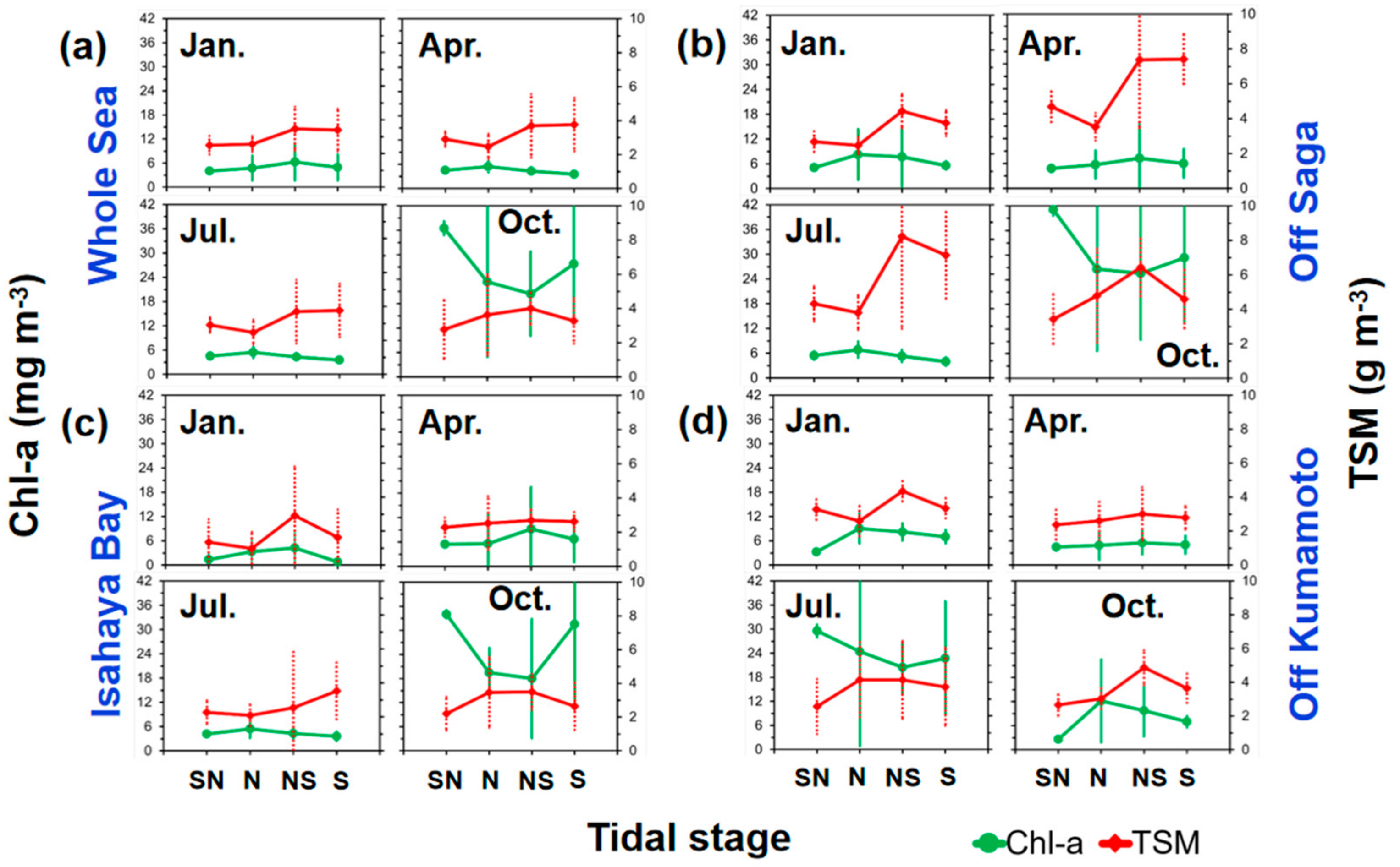
3.2. Monthly Climatology of Chl-a and TSM

The magnitude of Chl-a showed seasonal variations: it was generally lowest in winter (December, January, February), increased in spring (March, April, May), reached its height in summer (June, July, August), and then decreased in autumn (September, October, November) (Figure S3). For each season, the spring–neap tidal variability of monthly Chl-a showed similar patterns. Therefore, the middle months of each season were chosen as representative months (Figure 7). In winter and spring, Chl-a was much higher (>7 mg m⁻³) for the areas off Saga, Isahaya Bay and off Kumamoto, whereas in summer, high Chl-a expanded to the whole sea, and then began to be restricted to the areas off Saga, Isahaya Bay and off Kumamoto in October and November. The seasonal variability of TSM was much less than that of Chl-a. In addition, TSM was generally much higher (>6 g m⁻³) off Saga than that in other areas of the sea (<4 g m⁻³).

The relationship between the monthly Chl-a averaged over the spring–neap tidal cycle and the monthly river discharge were also examined (Figure 8) because river discharge was suggested to be one of the important factors for seasonal variation [10]. The monthly Chl-a was strongly and positively correlated with the monthly river discharge from all the rivers for the whole sea, off Saga, Isahaya and off Kumamoto (R² = 0.88, 0.89, 0.78 and 0.87; p < 0.05). The magnitude of Chl-a was much higher in summer and highest in July when the river discharge was highest. This suggests that river discharge could be one of the important factors for the large seasonal variability of Chl-a in all of the regions.

The relationship between monthly Chl-a and TSM over the spring–neap tidal cycle was separately investigated for the four areas (Figure 9; Figure 10;

Table 1. Statistics of the peaks within the spring–neap tidal cycles made for the monthly climatology of Chl-a and TSM for the whole sea, off Saga, Isahaya Bay, and off Kumamoto. A value of “1” indicates the occurrence of peaks.

Chl-a Peaks	Whole Bay				Off Saga				Isahaya Bay				Off Kumamoto
Month	SN	N	NS	S	SN	N	NS	S	SN	N	NS	S	SN	N	NS	S
Dec.			1			1					1			1
Jan.			1				1				1				1
Feb.				1		1				1						1
Mar.				1				1			1				1
Apr.		1				1				1				1
May			1			1					1				1
Jun.			1				1				1				1
Jul.	1				1				1				1
Aug.	1						1		1				1
Sep.			1				1				1				1
Oct.		1				1				1				1
Nov.			1				1					1			1
TSM Peaks	Whole Bay				Off Saga				Isahaya Bay				Off Kumamoto
Month	SN	N	NS	S	SN	N	NS	S	SN	N	NS	S	SN	N	NS	S
Dec.			1				1				1				1
Jan.			1				1				1				1
Feb.				1				1				1				1
Mar.				1				1				1				1
Apr.				1				1				1			1
May				1				1			1					1
Jun.				1				1				1				1
Jul.			1				1				1			1
Aug.			1				1					1			1
Sep.			1				1					1			1
Oct.			1				1				1				1
Nov.				1				1			1				1

). All the standard deviations were smaller than the difference of the spatial averages of the monthly data, suggesting that the differences of the spatial averages were significant. The variability of monthly Chl-a showed clear seasonal differences for all the four areas. The magnitude of Chl-a over the spring–neap tidal cycle was much higher (Figure 9) in July, which represented summer, than in other months, which corresponded to a higher river discharge in summer, especially in June (Figure 8). The Chl-a peaks within each tidal cycle occurred at SN or NS tides for summer, whereas the Chl-a peaks generally occurred at N or NS tides for other seasons, for all areas (Table 1). In contrast, the Chl-a peaks all occurred at N or NS tides for the annual climatology data. For the variability of monthly TSM over the tidal cycle, seasonal differences were relatively small compared with the regional difference as well as the monthly variation in Chl-a (Figure 9), and the TSM peaks all occurred at NS or S tide (Table 1).

The variability of the Chl-a:TSM ratios also showed seasonal and regional differences (Figure 10). For summer, the ratios were much higher and were almost above 1:600 for all areas, which was due to the high Chl-a (7.74~41.08 mg m⁻³). For other seasons, the ratios were generally highest at N tide and lowest at S tide and were almost below 1:600 for the whole sea and off Saga (Figure 10a,b), which was due to the high TSM (2.02~9.51 g m⁻³); in contrast for Isahaya and off Kumamoto (Figure 10c,d), the variability of the ratios over the tidal cycle was small, and the ratios were mostly between 1:600 and 1:275 due to the lower TSM.

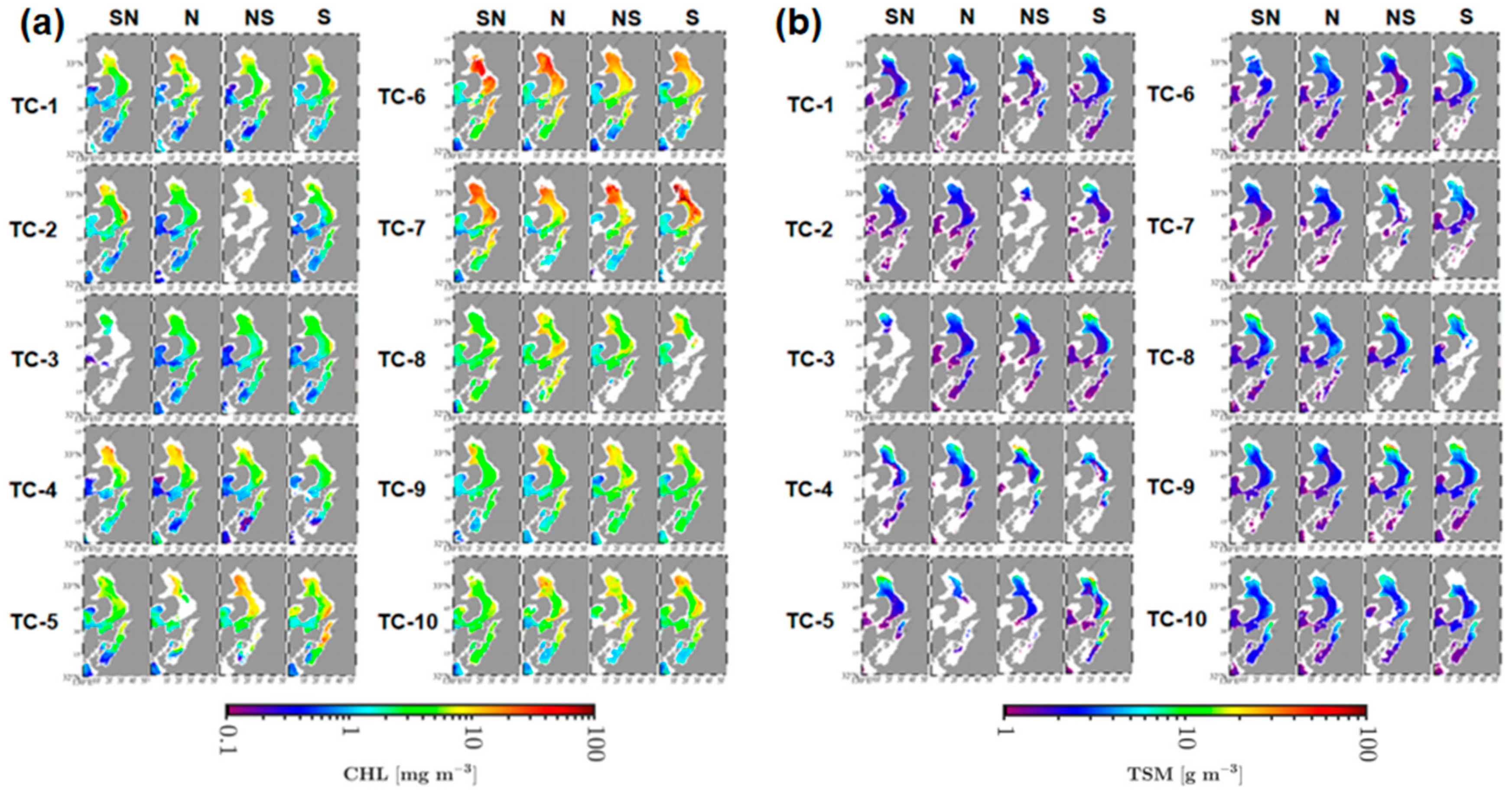
3.3. Individual Events of Spring–Neap Tidal Cycle Variability of Chl-a

The annual and monthly composite analysis indicated that there were strong spring–neap tidal cycles in Chl-a variation, which further varied regionally and seasonally. Therefore, the individual events of spring–neap tidal cycles from 2002 to 2017 were investigated. Because much of the Chl-a data were missing over the spring–neap tidal cycles, only 10 individual events had data available for all spring–neap tidal stages (

Table 2. Statistics of the spatially-averaged Chl-a and TSM values from the individual events of spring–neap tidal cycles, and river discharge during all ten tidal cycles. SD stands for standard deviation.

Tidal Cycle ID			Chl-a (mg m−3)				TSM (g m−3)						Chl-a:TSM						River Discharge (m3 s−1)
	Time Period	Month	SN	N	NS	S	Mean	SD	SN	N	NS	S	Mean	SD	SN	N	NS	S	Mean	Peak	Peak/Mean
TC-1	11/27/2003-12/11/2003	Dec.	6.06	7.72	7.85	6.53	7.04	0.88	3.07	2.64	5.27	4.58	3.89	1.41	1:472	1:365	1:511	1:495	198.43	311.33	1.57
TC-2	1/26/2004-2/10/2004	Feb.	8.06	3.73	8.66	4.04	6.12	2.60	2.45	2.29	2.27	2.78	2.45	0.10	1:304	1:613	1:262	1:689	138.46	161.54	1.17
TC-3	2/11/2004-2/23/2004	Feb.	2.73	3.36	3.23	3.49	3.20	0.33	3.59	2.52	3.34	4.79	3.56	0.56	1:1316	1:750	1:1034	1:1373	130.77	173.24	1.32
TC-4	3/26/2012-4/10/2012	Apr.	8.45	7.38	5.51	4.10	6.36	1.94	3.87	3.88	5.84	3.19	4.19	1.13	1:457	1:526	1:1059	1:777	429.34	1359.58	3.17
TC-5	4/28/2005-5/10/2005	May	3.98	7.39	11.29	8.19	7.71	3.00	4.15	3.17	3.15	5.83	4.07	0.57	1:1042	1:429	1:279	1:711	426.58	1533.01	3.59
TC-6	8/14/2010-8/28/2010	Aug.	30.81	20.96	12.54	12.20	19.13	8.78	2.64	3.29	2.57	3.97	3.12	0.40	1:86	1:157	1:205	1:325	255.59	428.56	1.68
TC-7	7/24/2008-8/5/2008	Jul.	17.58	12.78	17.89	32.97	20.31	8.76	2.26	2.68	4.98	3.47	3.35	1.46	1:129	1:210	1:278	1:105	289.92	639.89	2.21
TC-8	9/29/2003-10/12/2003	Oct.	4.94	8.17	6.07	6.67	6.46	1.35	5.11	3.55	5.58	5.49	4.93	1.06	1:1036	1:435	1:918	1:824	186.76	200.17	1.07
TC-9	10/13/2003-10/27/2003	Oct.	5.37	6.22	7.45	5.82	6.21	0.89	3.41	2.62	6.47	4.65	4.29	2.03	1:634	1:421	1:869	1:800	174.64	226.01	1.29
TC-10	11/16/2004-11/28/2004	Nov.	5.42	8.20	7.37	8.51	7.37	1.39	3.56	2.93	3.70	3.08	3.32	0.41	1:656	1:357	1:502	1:362	257.59	428.62	1.66

). The data were missing in some of the three target regional areas (Figure 11); thus, spatially-averaged Chl-a and TSM values were only calculated for the whole sea (Table 2).

The individual events of the spring–neap tidal cycles also suggested the seasonal variability of Chl-a over the spring–neap tidal cycle (Figure 11). In other words, the magnitude of Chl-a was generally low in winter (TC-1 to TC-3), spring (TC-4 to TC-5), and autumn (TC-8 to TC-10) and high in summer (TC-6 to TC-7); higher Chl-a (>7 mg m⁻³) generally occurred in the area off Saga, Isahaya Bay and off Kumamoto in winter and spring, expanded to the whole sea in summer, and was reduced to the area off Saga, Isahaya and off Kumamoto in autumn. This seasonal variability of Chl-a over the spring–neap tidal cycle was similar to that of the monthly climatology data.

The spring–neap tidal cycle variability of Chl-a and TSM was observed for the whole area (Figure 12; Table 2). In general, the spring–neap tidal variation was much smaller in winter, spring, and autumn than that in summer for Chl-a in terms of standard deviation. Daily river discharge data from two weeks before the first tidal stage (SN tide) was also used to investigate its influence on Chl-a (Figure 12). To quantify the variation of the river discharge, the ratio of the maximum:average of river discharge was calculated for each tidal cycle (Table 2). For TC-1 to TC-3, and TC-8 to TC-10, the river discharge peaks were low (ratio < 1.67), and Chl-a generally increased from SN to N or NS tide, and decreased during S tide; TSM was generally low during SN and N tide, and increased during NS or S tide. This variability of Chl-a and TSM was similar to that of the spatially-averaged monthly climatology data for the region off Saga and for the whole sea except for summer.

For the other tidal cycles, i.e., TC-4 and TC-7, the river discharge peaks were high (ratio > 1.67), and the river discharge peaks occurred before SN tide for TC-4, TC-6, and TC-7, while a peak occurred between NS and S tides for TC-5. For TC-5, the temporal variability of Chl-a and TSM was similar to that for TC-1 to TC-3, and TC-8 to TC-10, and the high river discharge had no influence on the Chl-a variation during the tidal stages before S tide. On the other hand, for TC-4, TC-6, and TC-7, after the high river discharge peak, Chl-a decreased continuously from SN to S tide except for TC-7. This may be due to the increase of Chl-a associated with high river discharges before the SN tide. TSM increased slightly from SN to N tide, then peaked at NS or S tide, which was similar to that exhibited for other tidal cycles. Furthermore, for TC-6 and TC-7, the Chl-a:TSM ratios (Table 2) were much higher than for other tidal cycles, indicating the dominance of phytoplankton in TSM for these two tidal cycles. These results indicate that high river discharge (ratio > 1.67) influenced the variation of Chl-a and TSM after during summer (TC-6 to TC-7), and that the occurrence of high river discharges can also influence the individual tidal cycles of Chl-a for other seasons (TC-4).

4. Discussion

4.1. Use of Satellite Data to Investigate the Spring–Neap Tidal Variations in Chl-a and TSM

Previous studies of the variability of Chl-a and TSM over spring–neap tidal cycles have primarily relied on in situ observations [3,4,17,23], and there are few studies based on satellite data [11,12,24]. In addition, previous studies of the Ariake Sea were only focused on the area off Saga, where the tidal range is larger than in other regions of the sea. Because of the observation method, those studies were limited to a few stations and a few spring–neap tidal cycles. Our study is different in that it relies on ocean color satellite data (MODIS-Aqua) to investigate the variability of Chl-a over the spring–neap tidal cycle, and we examine the tidal impacts on Chl-a for the whole Ariake Sea and specifically focus on three regional areas; i.e., off Saga, Isahaya Bay, and off Kumamoto. We used ocean color data from 2002 to 2017 to understand the annual and seasonal climatology as well as some events corresponding to spring–neap tidal cycles. This approach reveals that there are significant regional and seasonal differences in the Chl-a variability influenced by spring–neap tidal cycles. One of the known difficulties in using the standard MODIS Chl-a product for shallow coastal waters, such as the Ariake Sea, is the inadequacy of atmospheric correction schemes for obtaining accurate satellite-based Rrs that can be used to calculate Chl-a. It is also known that the present standard in-water algorithms for Chl-a estimates are biased in turbid waters. Here, we applied the Rrs recalculation method used in [25,18] and a local switching in-water algorithm for MODIS data to improve Chl-a retrievals in the Ariake Sea [18]. We also developed a TSM algorithm suitable for this area in this study. We have shown previously [18] that this recalculation method for Rrs and the improved empirical in-water algorithm significantly enhance the accuracy of the Chl-a retrievals from MODIS-Aqua. Our results showed the independent behavior of Chl-a and TSM over the spring–neap tidal cycle, which was consistent with previous studies for off Saga [13,14,17], suggesting that the influence of TSM on the satellite estimation of Chl-a was minimal, and the accuracy of our algorithms was adequate for our objective although imperfect.

To understand the influence of the spring–neap tidal cycle on Chl-a and TSM variability, we divided the spring–neap tidal cycle into four tidal stages (SN, N, NS and S tides). For each tidal stage, we produced annual and monthly climatology data and individual events of spring–neap tidal cycles of MODIS-Aqua Chl-a and TSM (2002–2017). This analysis made it possible for us to understand the seasonal and regional variations of tidal cycles of Chl-a and TSM, although there were much missing data in the spatial and temporal scales for many individual events of spring–neap tidal cycles over the 16 years.

4.2. Spatial and Seasonal Variability of the Spring–Neap Tidal Cycle

Tidal currents have been reported to be an important factor for the resuspension and transport of Chl-a and TSM into macrotidal environments, such as embayments, estuaries and tidal flats [4,23,26,27,28]. Using in situ data collected at several stations in the inshore area off Saga (October 2002–April 2003), in [17], the authors reported that Chl-a increased from N to NS and decreased during S tide, whereas TSM increased during S and decreased during N tide in the northern part of the Ariake Sea. The variability of TSM was explained by the resuspension of the sediment caused by the strongest tidal current during the S tide and re-sedimentation due to the weakest tidal current during N tide. The increase of Chl-a was explained by the increased light availability due to the reduction of TSM for the phytoplankton growth during N tide and the reduced light availability due to the increase of TSM during S tide [4,17].

Our results showed that the SN tidal resuspension in the Ariake Sea varied in space and time. Chl-a increased from SN to NS and decreased in S when TSM was high off Saga during fall, winter and spring when river discharge was low (Figure 7; Figure 8). This tidal cycle of Chl-a and TSM is consistent with a previous study [17]. The high TSM in this area reduces light availability and therefore limits phytoplankton growth, specifically during the spring tide when the resuspension of the sediment increased. This relation between the light availability and TSM is supported in a study by Ooshima et al. [29], in which it was reported that the attenuation coefficient in the surface water of the Ariake Sea was strongly and positively correlated with suspended sediment in winter, suggesting that light availability declines when the suspended sediment is higher. Moreover, the low Chl-a:TSM ratio (Figure 10b) during the spring tide indicates that the non-phytoplankton particles in particular suspended sediments are the dominant TSM during the S tide. In contrast, in [12], the authors reported that phytoplankton growth was enhanced due to the increased nutrients supplied by the spring tidal resuspension in German Bight. This suggests that the spring–neap tidal variability of Chl-a varied by regions. In Isahaya Bay and off Kumamoto also, Chl-a increased from SN to NS and decreased in S during fall, winter and spring, and the variation was still similar to that in the area off Saga (Figure 9c,d). However, the variations in TSM in terms of magnitude over the spring–neap tidal cycle were smaller than off Saga, suggesting that there may not be a large-scale resuspension of the sediment. This is consistent with the spatial variation of TSM (Figure 4; Figure 5; Figure 7), which shows a high TSM off Saga, with relatively low values in Isahaya Bay and off Kumamoto. The lower TSM in Isahaya Bay and off Kumamoto may be related to the reduction of the tidal flat of this area by the construction of a dike and sandy tidal flat caused by the lower tidal current, respectively [17]. The Chl-a:TSM ratio was higher than that off Saga, and Chl-a and TSM were highly correlated during the spring–neap tidal cycles (Figure 10). This indicates that the small variations in TSM were mostly composed of phytoplankton and that resuspended TSM was not the controlling factor for phytoplankton variation. Therefore, there might be different mechanisms, such as the advection of phytoplankton, which explain the spring–neap tidal variation in Chl-a and TSM for those regional areas. For example, in [27], it was reported that diatom blooms during winter were advected from the estuaries connected to off Saga to the middle parts of the Ariake Sea. In order to understand the mechanism for the spring–neap tidal variations in Chl-a for those two areas, further investigations may be required.

For the whole sea, the spring–neap tidal variability of Chl-a and TSM was similar to that off Saga (Figure 9 and Figure 10). This is probably due to the fact that both Chl-a and TSM values were higher off Saga than that in Isahaya Bay and off Kumamoto as well as in the middle-western areas. The similar spring–neap tidal variability of Chl-a and TSM between the whole sea and off Saga indicates that the influence of the tidal cycle-induced TSM was mostly important off Saga, whereas tidal cycle-driven variations in Chl-a were important over the whole sea. Even in the enclosed bay, it is clear that the tidal influence of the variability of Chl-a was different in each region.

4.3. Seasonal Influence of River Discharge to the Spring–Neap Tidal Variations in Chl-a

In estuaries and coastal systems, river discharge containing nutrients and suspended sediments can either positively or negatively influence Chl-a. The positive and negative relationship between river discharge and Chl-a is largely dependent on the dominant influence of either nutrients or irradiance on phytoplankton growth [30,31,32,33,34,35].

Our results showed that the monthly climatology data of river discharge were strongly and positively correlated with the spatially-averaged monthly climatology data of Chl-a over the spring–neap tidal cycle for the whole sea and regional areas (Figure 7). River discharge was also an important factor for the variability of Chl-a over the individual events of spring–neap tidal cycles, as our results showed that river discharge was probably the major driver of the variability of Chl-a in TC-4 and TC-6 (Figure 11). This suggests that river discharge promotes high phytoplankton growth in the Ariake Sea, which is consistent with previous studies [10,13].

The effects of spring–neap tidal cycle on the variability of Chl-a and TSM was not very clear during summer when the river discharge was high. The variation caused by the high river discharge during summer can mask the tidal cycle variation of Chl-a and TSM. The high correlation between Chl-a and river discharge indicates that the increase in Chl-a was caused by the possible nutrient input from the events of river discharge. We also observed that the Chl-a:TSM ratio was extremely high after the river discharge, and the values were often higher than 1:275–1:600, which is the range of phytoplankton-dominated water in Tokyo Bay [22]. The high ratio also reflects possible differences in the physiological conditions of phytoplankton after the river discharge.

5. Conclusions

As the spring–neap tidal variability of satellite Chl-a associated with TSM has not been investigated for a broad area and with a long-term data set, we investigated the spring–neap tidal variability of Chl-a on the basis of annual and monthly climatology data and individual events of spring–neap tidal cycles using an improved MODIS-Aqua data set (2002-2017). Spatially-averaged Chl-a and TSM and daily and monthly river discharge values were calculated to quantify the influence of TSM and river discharge on Chl-a for the whole sea and three regional areas (off Saga, Isahaya Bay and off Kumamoto).

The errors in MODIS-Aqua-derived Rrs and Chl-a for the Ariake Sea were effectively reduced by applying the methods in [11]. Therefore, we recalculated the 16-year MODIS-Aqua Rrs and Chl-a data with the same methods developed for this area used in [11]. Moreover, a local TSM algorithm was developed in this study, and then it was applied to the improved MODIS-derived Rrs to obtain the MODIS-derived TSM. The variability of Chl-a and TSM over the spring–neap tidal cycle off Saga was reasonable and was consistent with the field-based observations in previous studies, suggesting that the recalculated Chl-a and MODIS-derived TSM were separable.

The results of this study suggested seasonal and regional differences in the factors controlling the variability of Chl-a over the spring–neap tidal cycle. In general, the variability of Chl-a over the tidal cycle was controlled by river discharge during summer. In other seasons, it was controlled by the tidally resuspended TSM for off Saga and possibly by direct tidal transportation and tidal mixing in Isahaya Bay and off Kumamoto, respectively. In summary, this study suggests that satellite ocean color data offers an effective means for understanding the mechanisms of seasonal and regional Chl-a variability in coastal ecosystems that come under the influence of tides and river discharge.

This study also reveals that satellite ocean color data can discern the effects of spring–neap tidal cycles on Chl-a and TSM. However, we found different correlations between Chl-a and TSM in the Ariake Sea, confirming that the feature of spring–neap tidal cycles can vary in different areas. In addition, this is the first study to investigate the spring–neap tidal variability of Chl-a and TSM using satellite ocean color data in the Ariake Sea. Given the broad coverage and frequent sampling by satellites, our results reveal that satellite ocean color data can contribute significantly to our knowledge and understanding of the environmental dynamics caused by spring–neap tidal cycles in the Ariake Sea. The availability of these datasets offers the potential for the better management of the water quality of enclosed embayments such as the Ariake Sea.

References

1. Aoki, K.; Onitsuka, G.; Shimizu, M.; Matsuo, H.; Kitadai, Y.; Ochiai, H.; Yamamoto, T.; Furukawa, S. Interregional difference in spring neap variations in stratification and chlorophyll fluorescence during summer in a tidal sea (Yatsushiro Sea, Japan). Estuar. Coast. Shelf Sci. 2016, 180, 212–220. [Google Scholar] [CrossRef]
2. Azhikodan, G.; Yokoyama, K. Spatio-temporal variability of phytoplankton (Chlorophyll-a) in relation to salinity, suspended sediment concentration, and light intensity in a macrotidal estuary. Cont. Shelf Res. 2016, 126, 15–26. [Google Scholar] [CrossRef]
3. Cloern, J.E.; Powell, T.M.; Huzzey, L.M. Spatial and temporal variability in south San Francisco Bay (USA), II, Temporal changes in salinity, suspended sediments, and phytoplankton biomass and productivity over tidal time scales. Estuar. Coast. Shelf Sci. 1989, 28, 599–613. [Google Scholar] [CrossRef]
4. Koh, C.H.; Khim, J.S.; Araki, H.; Yamanishi, H.; Mogi, H.; Koga, K. Tidal resuspension of microphytobenthic Chlorophyll-a in a Nanaura mudflat, Saga, Ariake Sea, Japan: Flood−ebb and spring−neap variations. Mar. Ecol. Prog. Ser. 2006, 312, 85–100. [Google Scholar] [CrossRef]
5. Monbet, Y. Control of phytoplankton biomass in estuaries: A comparative analysis of microtidal and macrotidal estuaries. Estuaries 1992, 15, 563–571. [Google Scholar] [CrossRef]
6. Wofsy, S.C. A simple model to predict extinction coefficients and phytoplankton biomass in eutrophic waters. Limnol. Oceanogr. 1983, 28, 1144–1155. [Google Scholar] [CrossRef]
7. Feng, L.; Hu, C.; Chen, X.; Song, Q. Influence of the Three Gorges Dam on total suspended matters in the Yangtze Estuary and its adjacent coastal waters: Observations from MODIS. Remote Sens. Environ. 2014, 140, 779–788. [Google Scholar] [CrossRef]
8. Yamaguchi, H.; Ishizaka, J.; Siswanto, E.; Baek Son, Y.; Yoo, S.; Kiyomoto, Y. Seasonal and spring interannual variations in satellite-observed chlorophyll-a in the Yellow and East China Seas: New datasets with reduced interference from high concentration of resuspended sediment. Cont. Shelf Res. 2013, 59, 1–9. [Google Scholar] [CrossRef] [Green Version]
9. Gons, H.J.; Auer, M.T.; Effler, S.W. MERIS satellite chlorophyll mapping of oligotrophic and eutrophic waters in the Laurentian Gt Lakes. Rem. Sens. Environ. 2008, 112, 4098–4106. [Google Scholar] [CrossRef]
10. Ishizaka, J.; Kitaura, Y.; Touke, Y.; Sasaki, H.; Tanaka, A.; Murakami, H.; Suzuki, T.; Matsuoka, K.; Nakata, H. Satellite detection of red tide in Ariake Sound, 1998–2001. J. Oceanogr. 2006, 62, 37–45. [Google Scholar] [CrossRef]
11. Shi, W.; Wang, M.; Jiang, L. Spring-neap tidal effects on satellite ocean color observations in the Bohai Sea, Yellow Sea, and East China Sea. J. Geophysic. Res. 2011, 116. [Google Scholar] [CrossRef]
12. Su, J.; Tian, T.; Krasemann, H.; Schartau, M.; Wirtz, K. Response patterns of phytoplankton growth to variations in resuspension in the German Bight revealed by daily MERIS data in 2003 and 2004. Oceanologia 2015, 57, 328–341. [Google Scholar] [CrossRef] [Green Version]
13. Tsutsumi, H. Critical events in the Ariake Sea ecosystem: Clam population collapse, red tides, and hypoxic bottom water. Plankton Benthos Res. 2006, 1, 3–25. [Google Scholar] [CrossRef] [Green Version]
14. Hayami, Y.; Maeda, K.; Hamada, T. Long term variation in transparency in the inner area of Ariake Sea. Estuar. Coast. Shelf Sci. 2015, 163, 290–296. [Google Scholar] [CrossRef]
15. Unoki, S. Why did the tide and the tidal current decrease in Ariake Sea? Oceanogr. Japan 2002, 12, 85–96. (In Japanese) [Google Scholar] [CrossRef] [Green Version]
16. Unoki, S. The results of re-examining the recent decay of tide in Ariake Sea, based on smoothed data of observations. Oceanogr. Japan 2003, 12, 307–313. (In Japanese) [Google Scholar] [CrossRef] [Green Version]
17. Tanaka, K.; Kodama, M. Effects of resuspended sediments on the environmental changes in the inner part of Ariake Sea, Japan. Bull. Fish Res. Agency 2007, 19, 9–15. [Google Scholar]
18. Yang, M.M.; Ishizaka, J.; Goes, J.I.; Gomes, H.R.; Maúre, E.R.; Hayashi, M.; Katano, T.; Fujii, N.; Saitoh, K.; Mine, T.; et al. Improved MODIS-Aqua chlorophyll-a retrievals in the turbid semi-enclosed Ariake Sea, Japan. Remote Sens. 2018, 10, 1335. [Google Scholar] [CrossRef] [Green Version]
19. Gitelson, A.A.; Schalles, J.F.; Hladik, C.M. Remote chlorophyll-a retrieval in turbid, productive estuaries: Chesapeake Bay case study. Remote Sens. Environ. 2007, 109, 464–472. [Google Scholar] [CrossRef]
20. Le, C.; Hu, C.; Cannizzaro, J.; Duan, H. Long-term distribution patterns of remotely sensed water quality parameters in Chesapeake Bay. Estuar. Coast. Shelf Sci. 2013, 128, 93–103. [Google Scholar] [CrossRef]
21. Binding, C.E.; Bowers, D.G.; Mitchelson-Jacob, E.G. Estimating suspended sediment concentrations from ocean color measurements in moderately turbid waters; The impact of variable particle scattering properties. Remote Sens. Environ. 2005, 94, 373–383. [Google Scholar] [CrossRef]
22. Kishino, M.; Tanaka, A.; Ishizaka, J. Retrieval of Chlorophyll-a, suspended solids and colored dissolved organic matter in Tokyo Bay using ASTER data. Remote Sens. Environ. 2005, 99, 66–74. [Google Scholar] [CrossRef]
23. Ito, Y.; Katano, T.; Fujii, N.; Koriyama, M.; Yoshino, K.; Hayami, Y. Decreases in turbidity during neap tides initiate late winter large diatom blooms in a macrotidal embayment. J. Oceanogr. 2013, 69, 467–479. [Google Scholar] [CrossRef]
24. Valente, A.S.; da Silva, J.C.B. On the observability of the fortnightly cycle of the Tagus estuary turbid plume using MODIS ocean colour images. J. Mar. Sci. 2009, 75, 131–137. [Google Scholar] [CrossRef]
25. Hayashi, M.; Ishizaka, J.; Kobayashi, H.; Toratani, M.; Nakamura, T.; Nakashima, Y.; Yamada, S. Evaluation and improvement of MODIS and SeaWiFS-derived chlorophyll-a concentration in Ise-Mikawa Bay. J. RSSJ 2015, 35, 245–259, (In Japanese with English Abstract). [Google Scholar]
26. Demers, S.; Therriault, J.C.; Bourget, E.; Bah, A. Resuspension in the shallow sublittoral zone of a macrotidal estuarine environment: Wind influence. Limnol. Oceanogr. 1987, 32, 327–339. [Google Scholar] [CrossRef]
27. Black, K.S. Suspended sediment dynamics and bed erosion in the high shore mudflat region of the Humber Estuary, UK. Mar. Pollut. Bull. 1998, 37, 122–133. [Google Scholar] [CrossRef]
28. DeJonge, V.N.; Vanbeusekom, J.E.E. Wind-and-tide-induced resuspension of sediment and microphytobenthos from tidal flats in the Ems estuary. Limnol. Oceanogr. 1995, 40, 766–778. [Google Scholar]
29. Ooshima, I.; Abe, K. Estimation method for the attenuation coefficient in the surface layer of the Ariake Sea. Oceanogr. Japan 2005, 14, 593–600, (In Japanese with English Abstract). [Google Scholar] [CrossRef] [Green Version]
30. Lohrenz, S.E.; Dagg, M.J.; Whitledge, T.E. Enhanced primary production at the plume/oceanic interface of the Mississippi River. Cont. Shelf Res. 1990, 10, 639–664. [Google Scholar] [CrossRef]
31. Smith, W.O.; DeMaster, D.J. Phytoplankton biomass and productivity in the Amazon River plume: Correlation with monthly river discharge. Cont. Shelf Res. 1996, 16, 291–319. [Google Scholar] [CrossRef]
32. Dortch, Q.; Whitledge, T.E. Does nitrogen or silicon limit phytoplankton production in the Mississippi River plume and nearby regions? Cont. Shelf Res. 1992, 12, 1293–1309. [Google Scholar] [CrossRef]
33. Cloern, J.E.; Cole, B.E.; Wong, R.L.; Alpine, A.E. Temporal dynamics of estuarine phytoplankton: A case study of San Francisco Bay. Hydrobiologia 1985, 129, 153–176. [Google Scholar] [CrossRef]
34. DeMaster, D.J.; Knapp, G.B.; Nittrouer, C.A. Effect of suspended sediments on geochemical processes near the mouth of the Amazon River: Examination of biogenic silica uptake and the fate of particle-reactive elements. Cont. Shelf Res. 1986, 6, 107–125. [Google Scholar] [CrossRef]
35. Cole, J.C.; Caraco, N.F.; Peierls, B.L. Can phytoplankton maintain a positive carbon balance in a turbid, freshwater, tidal estuary? Limnol. Oceanogr. 1992, 37, 1608–1617. [Google Scholar] [CrossRef] [Green Version]
Figure 1. Location of Ariake Sea, Japan (a). The water depth of the bay is shown in light to dark blue (b). The seven main rivers, Rokkaku, Kase, Chikugo, Yabe, Kikuchi, Shira, Midori, and Kuma, are indicated by the arrows. The three regional areas—i.e., off Saga, Isahaya Bay, and off Kumamoto—are highlighted by the red boxes. The dike and the reclamation area within Isahaya Bay are represented by the brown line and meshed lines, respectively. The observation station for tidal level data of Ariake Sea, named Oura, is represented by the magenta filled circle.
Remotesensing 12 01859 g001
Figure 2. (a) Regression of the total suspended matter (TSM) algorithm based on the in situ TSM and Rrs667:Rrs547, and (b) the comparison between the in situ and Moderate Resolution Imaging Spectroradiometer (MODIS)-derived TSM data. The red lines are the regressions of the data in each plot, and the red dashed line represents the regression of the TSM algorithm. Equations of each regression and error statistics are also shown.
Remotesensing 12 01859 g002
Figure 3. Schematic flow of satellite composite data processing. The individual spring–neap tidal cycle, monthly and annual climatology of chlorophyll-a (Chl-a) and TSM were obtained from the MODIS-Aqua data set (2002–2017). Data of interannual and monthly, and interannual tidal cycle were the intermediate data. SN: spring to neap; N: neap; NS: neap to spring; S: spring.
Remotesensing 12 01859 g003
Figure 4. Satellite imagery of annual climatology of chlorophyll-a (Chl-a) (a) and total suspended sediment (TSM) (b). The whole sea, where spatially-averaged Chl-a and TSM were calculated, is marked in red.
Remotesensing 12 01859 g004
Figure 5. Satellite images of annual climatology of Chl-a (a) and TSM (b) over the spring–neap tidal cycle.
Remotesensing 12 01859 g005
Figure 6. Change of spatially-averaged annual climatology of Chl-a and TSM over the spring–neap tidal cycle (a) and the scattering plot (b) for the whole sea, off Saga, Isahaya Bay and off Kumamoto. The vertical lines in (a) represent the standard deviations of the spatial averages, and the dashed and dotted lines in (b) represent the Chl-a:TSM ratios of 1:600 and 1:275, respectively.
Remotesensing 12 01859 g006
Figure 7. Satellite images of monthly climatology of Chl-a (a) and TSM (b) over the spring–neap tidal cycle. The four months—i.e., Jan., Apr., Jul., and Oct.—represent winter, spring, summer, and autumn, respectively.
Remotesensing 12 01859 g007
Figure 8. Monthly climatology of Chl-a averaged over the spring–neap tidal cycle against the monthly climatology of river discharge. The data in winter, spring, summer, and autumn are represented by red, green, blue, and yellow markers, respectively. The lines are regression lines.
Remotesensing 12 01859 g008
Figure 9. The time-series of monthly climatology of spatially-averaged Chl-a over the spring–neap tidal cycle for (a) the whole Araike Sea, (b) off Saga, (c) Isahaya Bay, and (d) off Kumamoto. The vertical lines in each plot are standard deviations of spatial averages of all the interannual data.
Remotesensing 12 01859 g009
Figure 10. Scatter plots of monthly climatology of Chl-a and TSM over the spring–neap tidal cycle for the whole Sea (a), off Saga (b), Isahaya Bay (c) and off Kumamoto (d). The data for the four tidal stages—SN, N, NS and S tides—are represented by yellow, purple, magenta and light blue markers, respectively. The dashed and dotted line represents the Chl-a:TSM ratios of 1:600 and 1:275, respectively.
Remotesensing 12 01859 g010
Figure 11. Composite Chl-a (a) and TSM (b) images of the spring–neap tidal stages for the ten selected individual tidal cycles, i.e., TC-1 to TC-10. TC-1 to TC-3 were from winter, TC-4 to TC-5 were from spring, TC-6 to TC-7 were from summer, and TC-8 to TC-10 were from autumn.
Remotesensing 12 01859 g011
Figure 12. Time series of whole area-averaged Chl-a and TSM, and the daily river discharge for the ten representative individual events of tidal cycles: TC-1 to TC-3 (winter), TC-4 to TC-5 (spring), TC-6 to TC-7 (summer), and TC-8 to TC-10 (autumn). Chl-a and TSM in the four tidal cycles were represented by red and green markers, respectively. The river discharge, from two weeks before the tidal cycle to the end of the tidal cycle, is represented by the blue marked line. The average data was the average of all the daily data in each tidal stage. For each tidal cycle, the four Chl-a and TSM data from left to right were for SN, N, NS and S tides, respectively.
Remotesensing 12 01859 g012