Closing the Phenotyping Gap: High Resolution UAV Time Series for Soybean Growth Analysis Provides Objective Data from Field Trials

Abstract

Close remote sensing approaches can be used for high throughput on-field phenotyping in the context of plant breeding and biological research. Data on canopy cover (CC) and canopy height (CH) and their temporal changes throughout the growing season can yield information about crop growth and performance. In the present study, sigmoid models were fitted to multi-temporal CC and CH data obtained using RGB imagery captured with a drone for a broad set of soybean genotypes. The Gompertz and Beta functions were used to fit CC and CH data, respectively. Overall, 90.4% fits for CC and 99.4% fits for CH reached an adjusted R² > 0.70, demonstrating good performance of the models chosen. Using these growth curves, parameters including maximum absolute growth rate, early vigor, maximum height, and senescence were calculated for a collection of soybean genotypes. This information was also used to estimate seed yield and maturity (R8 stage) (adjusted R² = 0.51 and 0.82). Combinations of parameter values were tested to identify genotypes with interesting traits. An integrative approach of fitting a curve to a multi-temporal dataset resulted in biologically interpretable parameters that were informative for relevant traits.

1. Introduction

It has been demonstrated that close remote sensing approaches in combination with appropriate experimental designs and data integration can increase accuracy, precision, and throughput of on-field phenotyping experiments while also reducing cost and labor requirements [1]. These high throughput phenotyping approaches can also be implemented in crop breeding to determine architectural/morphological and physiological traits to aid early detection of desirable genotypes [2]. In these areas, the use of unmanned aerial vehicles (UAVs) is increasing steadily, as UAVs are suitable for use in complex field environments (e.g., muddy soil), are non-invasive, flexible in use (e.g., not restricted in use to particular field plots), and are available at a low cost [3]. UAV flights can be scheduled in function of the needs of the breeding program or experiment, using combinations of sensors that are suitable to investigate the traits of interest. In one of the most straightforward applications, canopy cover (CC) and canopy height (CH) data can be derived from images obtained using an RGB camera mounted on an UAV [4]. Canopy cover, defined as the ratio of the projected plant area to the total area considered, goes through changes from crop establishment to senescence. CC yields information regarding seedling emergence, early vigor, or senescence [5] and is therefore an important criterion in a breeding context [6]. Furthermore, CC data can be used to estimate canopy photosynthesis and transpiration [7] or to evaluate crop responses to abiotic stresses (e.g., drought stress; [8]). Canopy height (CH) is also dynamic and linked to growth, crop development, and yield [9,10].

One of the main advantages of UAV-based imaging approaches is the high precision and throughput for data acquisition and processing in comparison to the manual ruler measurements or scoring systems that have been traditionally used to analyze crop growth and development. By performing UAV flights throughout the entire growing season, accurate crop data can be obtained at a high spatio-temporal resolution, delivering dynamic information on crop growth and performance [11]. For example, in Yu et al. (2016) [12], data of five time points (using RGB and modified RGB-NIR imaging) were combined to classify soybean populations in different maturity groups and to estimate final yield. In Holman et al. (2016) [13], a method for deriving crop height and growth rate from multi-temporal 3D digital surface models of winter wheat field trials was developed. In Pugh et al. (2018) [14], UAV-based approaches to estimate height in sorghum and maize were determined and growth curves were fitted for different groups of breeding material. Similarly, in Chang et al. (2017) [15] sigmoidal curves were fitted to UAV-derived multi-temporal height data of sorghum. Multi-temporal height data (four flights) have also been used in combination with clustering analysis methods to detect different growth patterns in maize varieties [16].

These examples illustrate the value of multi-temporal data to describe crop growth and to predict specific parameters such as maturity, growth rate (in the above examples this was restricted to estimations considering two consecutive measurements) or yield. Up to now, however, little attention was paid to the biological interpretation of the growth curves built using UAV-based information. Nevertheless, the possibility for such interpretation represents one of the main advantages of this integrative approach. Multi-temporal data at high resolution can be of great value for sophisticated plant and crop modeling approaches. This is because crop models typically contain a large number of parameters that need to be estimated in an identifiable manner [17] based on preferentially large quantities of objective experimental (field) data. Furthermore, mathematical models can be fitted to multi-temporal data to link growth patterns to relevant environmental and developmental clues for a precise description of crop performance from sowing to harvest. This might also enable derivation of ‘hidden’ variables as phenome descriptors that are useful in a breeding context (e.g., determinacy).

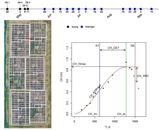
In this study, we demonstrate this concept using a soybean (Glycine max (L.) Merr.) experiment with 454 field plots comprising a diverse set of genotypes. More specifically, we fit mathematical models to multi-temporal data of CC and CH obtained for each plot and explore the possibilities of a global description of crop growth and development throughout the season in the context of breeding applications. First, CC and CH from each flight are estimated. Second, curves are fitted considering multi-temporal data per plot to extract biologically relevant information. Third, the correlation/complementarity of the model-based parameters obtained are evaluated. Fourth, parameters are examined for a possible relation to seed yield and maturity. Finally, an example to illustrate how the data could be used in a breeding context is developed to select interesting plots or to depict variability in the collection of genotypes evaluated.

2. Materials and Methods

2.1. Field Trial

An experimental field located in Melle (ILVO, Belgium, latitude 50.59 N, longitude 3.47 E) was used. The trial was established in 2018 in the context of the EU project EUCLEG (http://www.eucleg.eu/) and comprised 359 soybean genotypes randomized in a row-column-block augmented design in which three reference genotypes were replicated nine times, nine reference genotypes were replicated six times, and 13 reference genotypes were replicated three times. The remaining 334 genotypes were not replicated, rendering a total of 454 plots of 0.50 x 1.20 m (0.60 m²) or 0.80 x 0.75 m (0.60 m²), depending on the group to which the genotype belongs (Figure 1A). Within the 454 plots, there were 12 border plots (located between groups sections in Figure 1A) that were not considered in our analysis. This design was used to achieve the highest possible genotypic variation for an association mapping study in which genomic and phenotypic data will be combined. The genotypes used were classified beforehand in four groups that were sown on four different dates in an attempt to synchronize flowering of early maturing and late maturing types: April 20 (GP1), May 3 (GP2), May 8 (GP3), and May 11 (GP4) (Figure 1C). Each plot consisted of three rows; only the middle row was considered for the measurements. The seeds were inoculated with rhizobium bacteria (BiodozTM, De Sangosse, France) and the field was fertilized with 36 kg N ha^-1, 20 kg P2O5 ha^-1, 140 kg K2O ha^-1, and 20 kg MgO ha^-1. For weed control, 910 g ha^-1 pendimethaline and 72 g ha^-1 clomazone was applied directly after sowing (on the four sowing dates). A manual correction on June 13 was applied to ensure that no weeds developed that could hamper the growth of the crop or influence UAV-based measurements.

2.2. Data Acquisition

2.2.1. UAV Flights

Between May 28 and September 14, UAV flights were performed once per week when weather conditions allowed (Figure 1C), using a dodecacopter model Onyxstar HYDRA-12 (AltiGator, Belgium) equipped with a RGB (visible spectral range) camera (α6000, Sony Corporation, Japan), with 6000 × 4000 pixels and a 35 mm lens (f/1.8 Sony Corporation, Japan). Per flight, a set of nadir images was collected from a height of 30 m above ground level (raw image resolution of 3.35 mm/pix), ensuring an overlap of 70% in both directions (forward-longitudinal-lap and side-lap) at a flight speed of 2.5 m/s. The RGB camera settings (shutter speed, aperture, and ISO) were adjusted before each trial, set in manual mode, and triggered automatically according to the designed flight route. Depending on the weather conditions (light intensity and wind), shutter speed was ≤1/1000 s and ISO was ≤800.

In total, 14 flights were executed around 13:00h (local time) and the required images were captured in less than 20 minutes. A graph thermal time (°C d) versus time for the growing season is included in the Supplementary Materials (Figure S1). Correction for white balance and exposure was applied to the images. Processing of the 14 sets of images and building of geo-referenced orthophotos and digital elevation models (DEMs) were done using Agisoft Photoscan v1.2.6 Professional Edition (Agisoft LLC, Russia) based on 10 Ground Control Points (GCPs) geo-referenced with an RTK GPS (Stonex S10 GNSS, Stonex SRL, Italy). The resulting RGB ortho-mosaicked images had a planimetric spatial resolution of 0.5 cm; the DEMs had an altimetric resolution of 1.25 cm. Spatial resolutions were defined when both products (orthophotos and DEMs) were exported to ensure that products from different flights had the same resolution. Digital elevation models were used to build a Canopy Height Model (CHM) for each date. A triangulated irregular network (TIN) interpolation of 25 GCPs distributed all over the trial was used as Digital Terrain Model (DTM). The CHM was obtained by subtracting the DTM from the DEM.

2.2.2. On-Ground Measurements

Traits commonly recorded by breeders to track growth and reproductive development were monitored during the growing season by experienced UAV operators. The percentage of emergence was calculated by dividing the number of emerged plants by the total seed density. Plots with a percentage of emergence lower than 50% were discarded. The reproductive stage (from R1 to R6) was recorded at five fixed dates for each plot, as described in Fehr and Caviness (1977) [18]. The date of maturity (R8) was recorded separately by frequent visits to the field trial at the end of the growing season. R1 corresponds to beginning bloom (one open flower at any node on the main stem) and R8 is full maturity (95% of the pods have reached their mature pod color). As the R1 stage of each of the plots did not always coincide with one of the five time points considered, we estimated it by linear regression of the reproductive stage (five time points) and thermal time at time of scoring. Thermal time was calculated as the daily accumulation of the difference between the mean daily temperature and a base temperature (6 °C) over a period of time (°C d). Plots for which R² was lower than 0.7 were discarded, as the determination of R1 stage was considered inaccurate. In total, 324 plots remained for further analysis after the discards related to emergence rate and R1 stage.

At maturity, five plants of the middle row of each plot were harvested by hand and were threshed together to determine average seed yield and number of seeds per plant.

2.3. Data Handling and Statistical Analysis

The different analysis steps are presented schematically in Figure 1D. First, canopy cover (CC) and canopy height (CH) data were extracted per plot. Second, sigmoid growth curves were fitted to CC and CH data using the 14 time points available and variables were estimated (see Section 2.3.2). Third, a principal component analysis (PCA) was carried out to investigate the complementarity of parameters describing the genotypes. Last, predictive models were built for seed yield (SY) and R8 using multiple linear regression (MLR) models.

QGIS v2.18.26-Las Palmas (QGIS Geographic Information System; Open Source Geospatial Foundation Project) was used to extract information from the images. Georeferenced polygons with the dimension of the plot middle row were defined in QGIS to ensure that data were extracted from the same location for each and every flight and that only the information of the middle row was captured (Figure 1). The curve fitting and the statistical analyses were carried out in R v3.5.1 using RStudio v1.1.456 (RStudio: Integrated Development Environment for R, RStudio Inc., USA) coding customized functions for fitting the curves and using packages such as FactoMineR and optimx for the PCA and optimization of the functions, respectively. These customized functions can be shared, upon request to the corresponding author.

2.3.1. Canopy Cover and Canopy Height

The canopy cover was calculated per time point and plot using the Excess Green vegetation index (ExG, [19]). Pixels corresponding to vegetation were differentiated from pixels corresponding to soil (Figure 1B) using a simple thresholding, and the proportion of pixels classified as vegetation was then calculated.

CHMs were built for each date (described in Section 2.2.1) and used to estimate the 90th percentile (P90) of the canopy height for each plot. Only pixels corresponding to vegetation (the pixel classification described in the previous paragraph was used to build masks) were considered for this calculation.

2.3.2. Model Fitting and Parameter Estimation

Canopy cover and canopy height data extracted for the 14 time points considered (timeline Figure 1C) were used to fit curves describing their temporal evolution in 324 plots. After reaching the maximum value, subsequent time points were only considered for fitting if the difference in value was not greater than 10% from the maximum canopy cover, and 20% from the maximum plant height. When plants get older and start to senesce, they gradually lose leaves and the CC and/or CH is reduced. These criteria prevented any excess influence of these changes on the CC and/or CH fits, as our interest was to fit the sigmoid part of canopy development. The last two time points were excluded by default, because senescence was already observed in a majority of plots. This implies that a maximum of 12 time points were included in each fit. For the fits, we chose curves that have parameters that are biologically interpretable [20] and that reach a “plateau” that defines growth stop.

For the canopy cover (CC) data the Gompertz function [21] was used. In this function, an initial value (at the beginning of the growing season) is assumed. In the present experiment, the first drone flight was carried out when the plants had already emerged (canopy cover >0%). From the Gompertz fits, two parameters were extracted (Figure 2A, formula 1): maximum cover (CC_Cmax) and thermal time when growth rate was maximal (CC_tm). The Gompertz function used for CC has the following equation:

$$CC=CC\_C_{max}{e}^{e^{-k\left(t-CC\_t_m\right)}},$$

(1)

where CC_Cmax [%] is the maximum CC value attained, t is the thermal time [°C d], k [°C-1 d-1] is a constant that determines the curvature of the growth pattern, and CC_tm [°C d] is the inflection point at which the growth rate reaches its maximum value.

For the canopy height (CH) data, the Beta function defined in Yin et al. (2003) [22] was chosen because it has more flexibility than Gompertz at the beginning of the growing season. In addition, for the Beta function the limit is not known in advance, while the CC data values are restricted by definition to the range 0–100. The Beta function was used to estimate the following parameters (Figure 2B, formula 2): maximum height (CH_Hmax), thermal time when maximum canopy height was achieved (CH_te), and thermal time when the growth rate was maximal (CH_tm). The Beta function used for CH has the following equation:

$$CH=CH\_H_{max}\left(1+\frac{CH\_t_e-t}{CH\_t_e-CH\_t_m}\right){(\frac{t}{CH\_t_e})}^{\frac{CH\_t_e}{CH\_t_e-CH\_t_m}}$$

(2)

where CH_Hmax [m] is the maximum value of CH reached at CH_te [°C d], t is the thermal time [°C d], and CH_tm [°C d] is the inflection point at which the growth rate reaches its maximum value.

The accuracy of the fitting was evaluated by adjusted R² (CC_RsqA and CH_RsqA). Plots with an adjusted R² lower than 0.70 were discarded, resulting in 291 remaining plots (when both datasets were merged) for further analysis.

2.3.3. Derived Phenotypic Parameters

Using the fitted growth curves, additional phenotypic parameters were derived (Figure 2). These phenotypes are more difficult to measure in the field. From the CC growth function, we calculated the maximum absolute growth rate (CC_AGRmax) as the first derivative of the function (which is the slope), the canopy cover six weeks after emergence (CC_6W; related to the capacity of the genotype to suppress weeds) and the thermal time needed to reach 75% of full canopy cover (CC_75PCT; related to canopy closure).

From the CH growth function, maximum absolute growth rate (CH_AGRmax) was calculated and the degree of determinacy (CH_DET) was estimated by calculating the thermal time difference between the CH_te and the R1 stage (based on visual scores). According to this calculation, a high CH_DET value indicates a longer period of growth and a lower level of determinacy.

Finally, the senescence rate was calculated as the difference between the maximum value of the fitted curve and the average value of the last two time points. Calculations were performed for CC and CH (CC_SNC and CH_SNC, respectively).

To determine whether a significant difference is present between the groups, a multiple pairwise comparison using Wilcoxon rank sum was carried out for all phenotypic variables.

2.3.4. Relations Among Phenotypic Parameters

A PCA analysis was performed to investigate the relation between the different phenotypic parameters and to find out which ones were correlated or complementary. Twelve phenotypic parameters obtained from the UAV imagery were included (

Table 1. Overview of the phenotypic parameters.

Data Source		Abbreviation	Description
UAV Orthophoto	Canopy Cover (CC)	CC_tm	Thermal time when maximum growth rate is achieved
		CC_Cmax	Maximum cover
		CC_AGRmax	Maximum absolute growth rate
		CC_6W	Cover percentage after six weeks emergence
		CC_75PCT	Thermal time when 75% of cover is achieved
		CC_SNC	Senescence rate calculated with CC data (CC_Cmax – average cover two last time points)/CC_Cmax
Digital Elevation Model	Canopy Height (CH)	CH_tm	Thermal time when maximum growth rate is achieved
		CH_Hmax	Maximum height
		CH_te	Thermal time when CC_Hmax occurred
		CH_AGRmax	Maximum absolute growth rate
		CH_DET	Determinacy calculated as CH_te – R1
		CH_SNC	Senescence rate derived from CH data (CC_Hmax—average height two last time points)/CC_Hmax
Breeders	Field observations	EP	Percentage of emergence
		SY	Seed yield
		R1	Thermal time when R1 stage starts (beginning bloom)
		R8	Thermal time when R8 stage is reached (full maturity)

) and three on-ground determined variables (as quantitative supplementary variables). The four groups (GP1 to GP4) were considered together. To prevent a specific GP from determining the results, an equal number of plots per group were chosen at random (avoiding plots that corresponded to replicates of the same genotype) to ensure a balanced dataset. This resulted in a set of 148 plots. Pairwise correlations were also calculated between the parameters for the same set of plots.

In addition, pairwise correlations per GP were estimated separately. When one genotype was represented by more than one plot (see Section 2.1), only one was retained to prevent the replicates from influencing the correlation output.

2.3.5. Seed Yield and R8 Stage Prediction from UAV Data

From a breeding perspective it is important to know which variables act as driver for seed yield (SY) or influence the thermal time needed to reach maturity (R8). Therefore, two backward multiple linear regression (MLR) models were built for SY and R8 with different sets of variables. The first MLR model was built using the values of the 12 phenotypic parameters that were determined from the curve fitting, whereas the second MLR model was built on the raw data of the 14 time points (flights). In both cases, the group classification was included as a dummy variable for the basic model to be used as starting point. To avoid collinearity between the phenotypic variables in building the first MLR model, variables were selected based on expert knowledge. Consequently, the variables CC_6W and CH_DET were discarded as they are highly correlated with CC_75PCT and CH_te. For the second MLR model, no expert variable selection was done since the raw data set is difficult to interpret in terms of redundancy. The MLR models were built using subset selection regression including a 10 k-fold cross validation. The variables for both datasets were normalized. In each subsequent step, the number of variables included was increased by one, while considering all possible combinations of variables and the best model was chosen based on the lowest RMSE.

3. Results

3.1. Model Fitting for Canopy Cover and Canopy Height

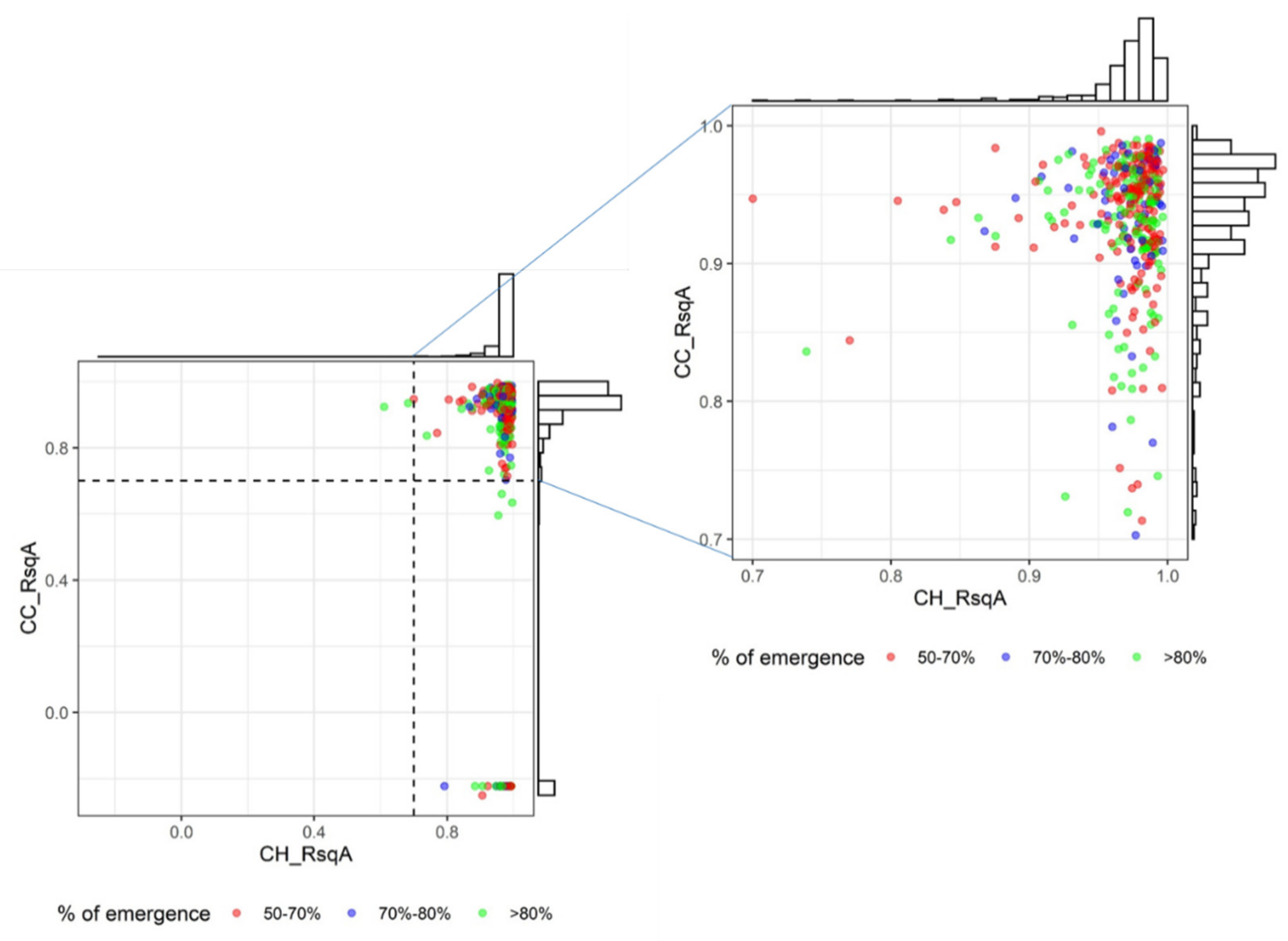
In an exploratory data analysis of CC and CH data, after discarding plots with emergence <50% or R² < 0.7 in the estimation of R1 stage, different growth patterns per group were observed (data not shown), which was confirmed in the subsequent analysis.

Fitting of CC data using the Gompertz function resulted in 90.4% fits with an adjusted R² > 0.70. For the CH data to which the Beta model was fitted, 99.4% fits had an adjusted R² > 0.70. Combining the 0.7 limits for both fits, rendered 291 plots that fulfilled both criteria (89.8%), with a median CC_RsqA of 0.95 and CH_RsqA of 0.98 (Figure 3).

The parameter values for CC are presented in

Table 2. Mean, median, standard deviation (Stdev) and coefficient of variation (cv) of the phenotypic parameters derived from fitting the canopy cover data. Data are presented per group (GP1-4). For the abbreviations, see Table 1.

		UAV Parameters
		Estimated Parameters		Derived Parameters
		CC_tm (°C d)	CC_Cmax (%)	CC_AGRmax (% °C−1 d−1)	CC_6W (%)	CC_75PCT (°C d)	CC_SNC (-)
GP1	Mean	390	94.1	0.518	79.5	509	0.315
	Median	446	94.2	0.660	65.8	525	0.074
	Stdev	69	2.6	0.300	21.8	64	0.230
	cv	15.9	2.8	45.3	36.7	11.9	129.5
GP2	Mean	390	94.1	0.518	79.5	509	0.315
	Median	378	94.2	0.475	81.0	499	0.238
	Stdev	51	2.3	0.217	11.5	65	0.300
	cv	13.1	2.4	41.9	14.5	12.8	95.1
GP3	Mean	329	95.3	0.807	93.3	401	0.493
	Median	324	95.6	0.761	94.6	372	0.483
	Stdev	59	1.8	0.293	5.2	57	0.262
	cv	17.9	1.9	36.6	5.5	14.3	53.1
GP4	Mean	306	94.6	0.689	90.6	399	0.715
	Median	299	94.8	0.577	93.4	379	0.815
	Stdev	56	3.1	0.348	9.1	81	0.235
	cv	18.2	3.3	50.4	10.1	20.3	32.9

. For CC_tm (°C d) the median values ranged from 299 to 446; for CC_Cmax (%) the values ranged from 94.2 to 95.6. On average, CC_tm was lower for the later-sown groups GP3 and GP4 than for the groups GP1 and GP2 (Figure 4A).

For CH, the parameter values are presented in

Table 3. Mean, median, standard deviation (Stdev) and coefficient of variation (cv) of the phenotypic parameters derived from fitting the canopy height data. Data are presented per group (GP1-4). For the abbreviations, see Table 1.

		UAV Parameters
		Estimated Parameters			Derived Parameters
		CH_tm (°C d)	CH_Hmax (m)	CH_te (°C d)	CH_AGRmax (m °C−1 d−1)	CH_DET (°C d)	CH_SNC (-)
GP1	Mean	753	0.96	1333	0.00118	636	0.274
	Median	735	0.93	1312	0.00118	595	0.245
	Stdev	113	0.21	258	0.00025	293	0.139
	cv	15.1	21.5	19.3	20.9	46.0	50.9
GP2	Mean	695	0.95	1280	0.00121	675	0.336
	Median	699	0.96	1272	0.00119	644	0.261
	Stdev	112	0.18	248	0.00025	262	0.181
	cv	16.1	19.2	19.4	21.0	38.8	53.9
GP3	Mean	627	0.91	1029	0.00151	402	0.427
	Median	609	0.91	989	0.00149	389	0.379
	Stdev	72	0.14	150	0.00026	156	0.173
	cv	11.6	15.0	14.6	16.9	38.7	40.4
GP4	Mean	535	0.77	897	0.00149	340	0.637
	Median	547	0.76	901	0.00155	339	0.639
	Stdev	92	0.18	170	0.00035	181	0.186
	cv	17.2	23.3	19.0	23.5	53.2	29.1

. For CH_tm (°C d) this resulted in a range from 547 to 735, for CH_Hmax (m) from 0.76 to 0.96 and for CH_te (°C d) from 901 to 1312.

To complete the results presented in Figure 4; Figure 5, we checked whether the differences between groups were significant. For CC_Cmax, the only pair with a significant difference was GP2-GP3. All pairwise comparisons were significant for CC_tm.

In the case of CH_Hmax only GP4 showed significant differences with the other three groups. All six pairwise combinations were significant for CH_tm. Almost the same results were found for CH_te— except GP1-GP2, which was not significantly different.

3.2. Extra Phenotypic Parameters Derived from the Fitted Curves

As models were fitted to the time series, we could derive phenotypic parameters that correspond to traits that are hard to observe or measure in the field such as growth rate, weed suppression, determinacy or senescence.

The median of the CC_AGRmax (% °C⁻¹ d⁻¹) ranged from 0.475 to 0.761 when different GPs were considered. Although the four groups differed in CC_AGRmax (Figure 4C) almost all their plots reached high CC_Cmax > 90–95% (Figure 4B) as can be expected because standard deviations are <3.1%. Based on the canopy cover growth curve, a value related to weed suppression (Table 2 and Figure 4D) was derived by estimating the percentage of canopy cover reached six weeks after emergence (CC_6W (%)). The median values varied between 65.8 and 94.6 for the four groups considered. Strikingly, a large spread of values in GP1 and GP2 was observed, indicating a slow canopy development for some of the genotypes contained in these groups. Thermal time values when 75% of canopy coverage was reached (CC_75PCT; °C d) ranged from 372 to 525, meaning that GP1 and GP2 needed more time (were slower) to close canopy. A group effect was also present here, with considerable variation found within each group (Figure 4D,E).

The median values for CH_AGRmax (m °C⁻¹ d⁻¹) ranged from 0.00118 to 0.00155. The two groups with the highest CH_AGRmax were GP3 and GP4; they reached their maximum height earlier (lower CH_te), but the other two groups showed a higher CH_Hmax (Figure 5B–D). The determinacy values are summarized in Table 3 and Figure 5E. This variable indicates how long the plants kept growing after reaching R1. The median CH_DET values ranged from 339 to 644 (°C d). Figure 5E shows that GP3 and GP4 contained more determinate genotypes than GP1 and GP2, but again with a large variation.

Finally, based both on the canopy cover and the height fits, senescence was estimated (Table 2; Table 3 and Figure 4F and Figure 5F). These senescence parameters describe the ratio of decrease for CC and CH between the maximum value derived from the model fitting and the average value of the two last flights. In other words, the higher the values, the more senescence was observed. For CC_SNC median values ranged from 0.074 to 0.815, and in the case of CH_SNC, the median values ranged from 0.245 to 0.639. GP4 showed the highest CC_SNC and CH_SNC values followed by GP3 (Figure 4F and Figure 5F). Taken together with results for determinacy, we can conclude that GP3 and GP4 contained more determinate genotypes that senesce earlier in the environment tested. The histograms of all parameters are available in the Supplementary Materials (Figure S2 and Figure S3).

The analysis to identify significant differences between groups resulted in the following. In the case of CC_AGRmax, all six pairwise comparisons were significant, except GP1-GP4. For CC_6W and CC_SNC, all pairwise comparisons were significant. For CC_75PCT, all pairwise comparisons significant except for the comparison GP3-GP4. In the case of CH_AGRmax the two pairs that were not significantly different were GP1-GP2 and GP3-GP4. For CH_DET and CH_SNC all comparisons were significant except for GP1-GP2.

3.3. Relations between Phenotypic Parameters

To visualize the relations and complementarity among all phenotypic data, a PCA was carried out (Figure 6) and pair-wise correlations were calculated (Figure 7). The PCA (for all GP together) explained 81.7% of the variance present using the first four dimensions. Positively correlated variables were CC_75PCT with CC_tm, CH_DET with CH_tm and CH_SNC with CC_SNC. Examples of negatively correlated variables were CC_75PCT and CC_6W (Figure 6A and Figure 7E). Variables that show an orthogonal relation in the PCA graphs provide complementary data, for example CH_Hmax and CC_6W, indicating that the maximum height achieved is not correlated with the canopy development in early stages. Based on the contributions of the variables to the two first principal components (Figure 6A), the most important variables to explain the variability in the data set were CH_tm, CH_te and CC_75PCT for the first principal component and CH_Hmax and CC_AGRmax for the second principal component. The total variance in the PCA is further explained by the CH derived parameters than the CC ones (57.9% versus 42.1%, data not shown). A large overlap between GPs was observed when the plots were plotted in the two first dimensions of the PCA (Figure 6B) and similar patterns were observed when correlations were calculated per GP (Figure 7), indicating no clear-cut differentiation among GPs.

SY, R, and R8 values obtained using ground-based methods were plotted on top of the PCA carried out with the phenotypic variables derived from UAV-based data (Figure 6, red arrows). SY and R8 are positively correlated, both with each other as well as largely with CH_te, CH_tm, and CH_DET. SY and R8 are negatively correlated with CC_SNC and CH_SNC. This is consistent with the results shown in Figure 7. The low correlation of CC_max with all variables was expected, as all plots reached a high maximum canopy cover, resulting in a small variance. Lower correlations between SY, R1, and R8 with all the other variables were observed for GP4 compared to the other groups (Figure 7D).

3.4. Linking UAV-Based and Breeder Information

In

Table 4. Statistics and coefficients of the normalized variables for the MLRs for seed yield (SY) and R8 stage based on the phenotypic parameters and the raw flight data.

	RMSE	Adj R2	Int.	GP2	GP3	GP4	Variables Included in Model
SY							CC_SNC	CH_te	CH_AGRmax
	4.650	0.486	17.68	−2.94	−7.55	−6.13	−1.70	1.74	1.77
							CC_246	CC_228	CH_199
	4.579	0.501	18.31	−3.96	−9.10	−6.09	2.05	0.93	1.05
							CC_157	CC_199
							−0.92	−0.59
R8							CC_SNC	CH_Hmax	CH_tm
	63.463	0.804	1777.51	−112.73	−169.99	−208.54	−44.05	14.69	17.60
							CC_Cmax
							10.29
							CC_246	CH_235	CC_206
	56.944	0.842	1790.79	−122.79	−200.07	−221.49	43.234	30.626	14.227
							CC_228	CC_177	CC_171
							11.07	−24.76	30.40
							CH_164	CH_177
							−28.45	16.67

, the results of the four MLR models built for SY and R8 with different sets of variables are presented. Higher adjusted R² value and lower RMSE were obtained for R8 compared to SY. The similar adjusted R² between the MLR models based on different datasets indicated that SY and R8 could be estimated with similar performance either using the phenotypic parameters (from curve fitting) or the 14 time points (flights), with a trend towards a better prediction based on the raw data, but resulting in models that are less interpretable.

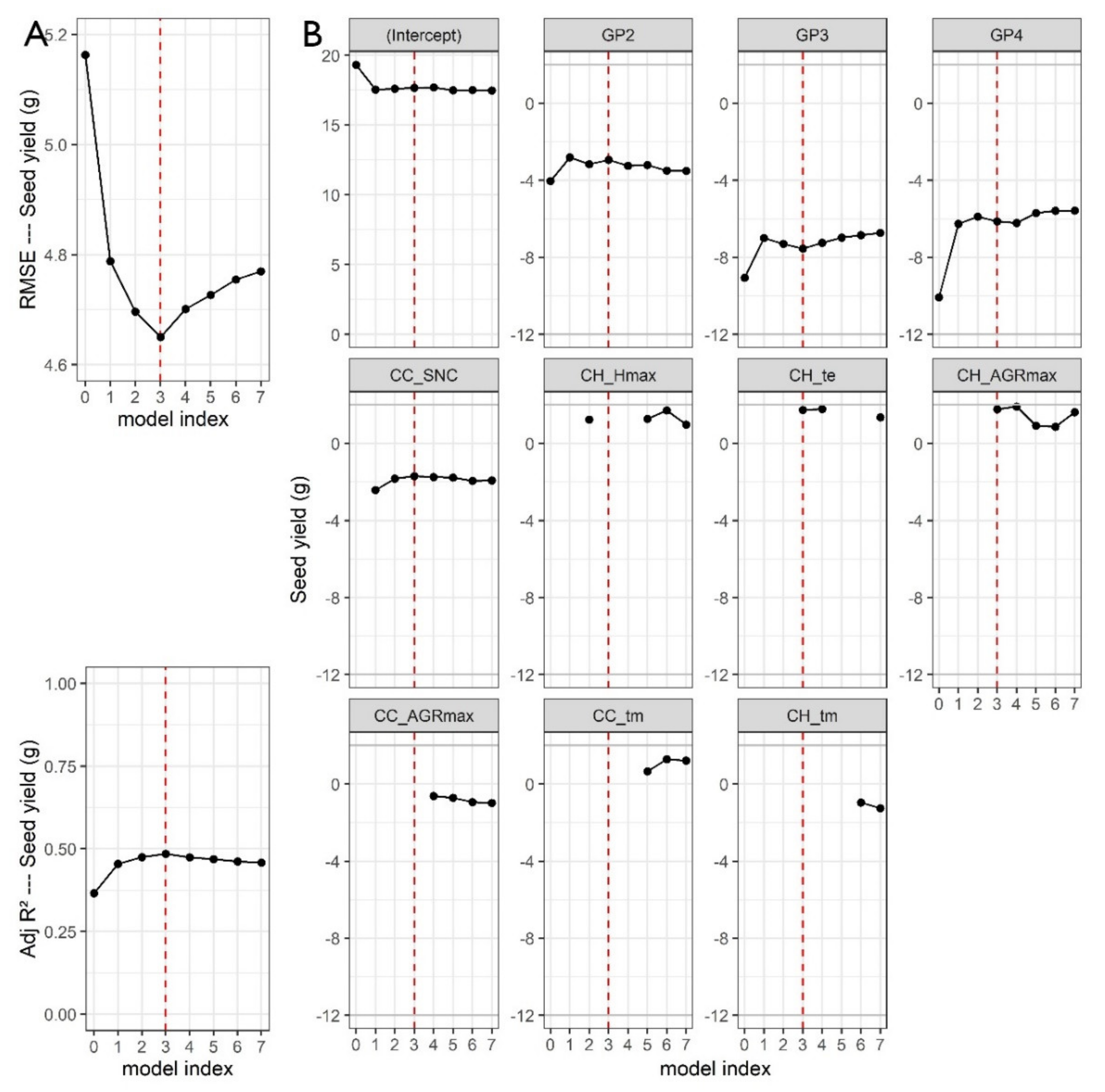
When UAV phenotypic variables were used in the MLR building, the best result for SY was achieved when using three variables: CC_SNC (senescence ratio), CH_te (thermal time when maximum height is reached) and CH_AGRmax (maximum growth rate) with an RMSE of 4.65 g (9% improvement compared to the basic model). In Figure 8A, the RMSE evolution in response to adding a variable is visualized, whereas Figure 8B shows the intercept, the coefficients for each GP and the variables included in each model. The red dashed line indicates the best model with three extra variables compared to the basic model. Figure 8 and Table 4 demonstrate that the models for SY show stable coefficients for the groups, independently of the number of variables added. This indicates a separate effect explained by the dummy variables. The coefficients for CC_SNC, CH_te and CH_AGRmax in the final model have the same magnitude and have consequently comparable importance. The negative coefficient for CC_SNC indicates that an earlier senescence reduces SY. A positive coefficient for CH_te and CH_AGRmax suggests that a later date to achieve the maximum canopy height and a higher AGRmax are linked with a higher SY In the case of R8, a similar figure is presented and a best model with four phenotypic variables resulted in a RMSE of 63.46 (23% improvement compared to the basic model). The variables included in the model were CC_SNC, CH_Hmax, CH_tm and CC_Cmax. Figures for the other three MLR models are included in the Supplementary Materials (Figures S4–S6).

In the case of SY, using the 14 time points, five variables were selected as the best model obtaining a RMSE of 4.58 g (11% improvement compared to the basic model). Four of these variables corresponded to CC data. For R8, eight variables were selected including CC and CH data and RMSE was 56.94 (improvement of 31% compared to the basic model).

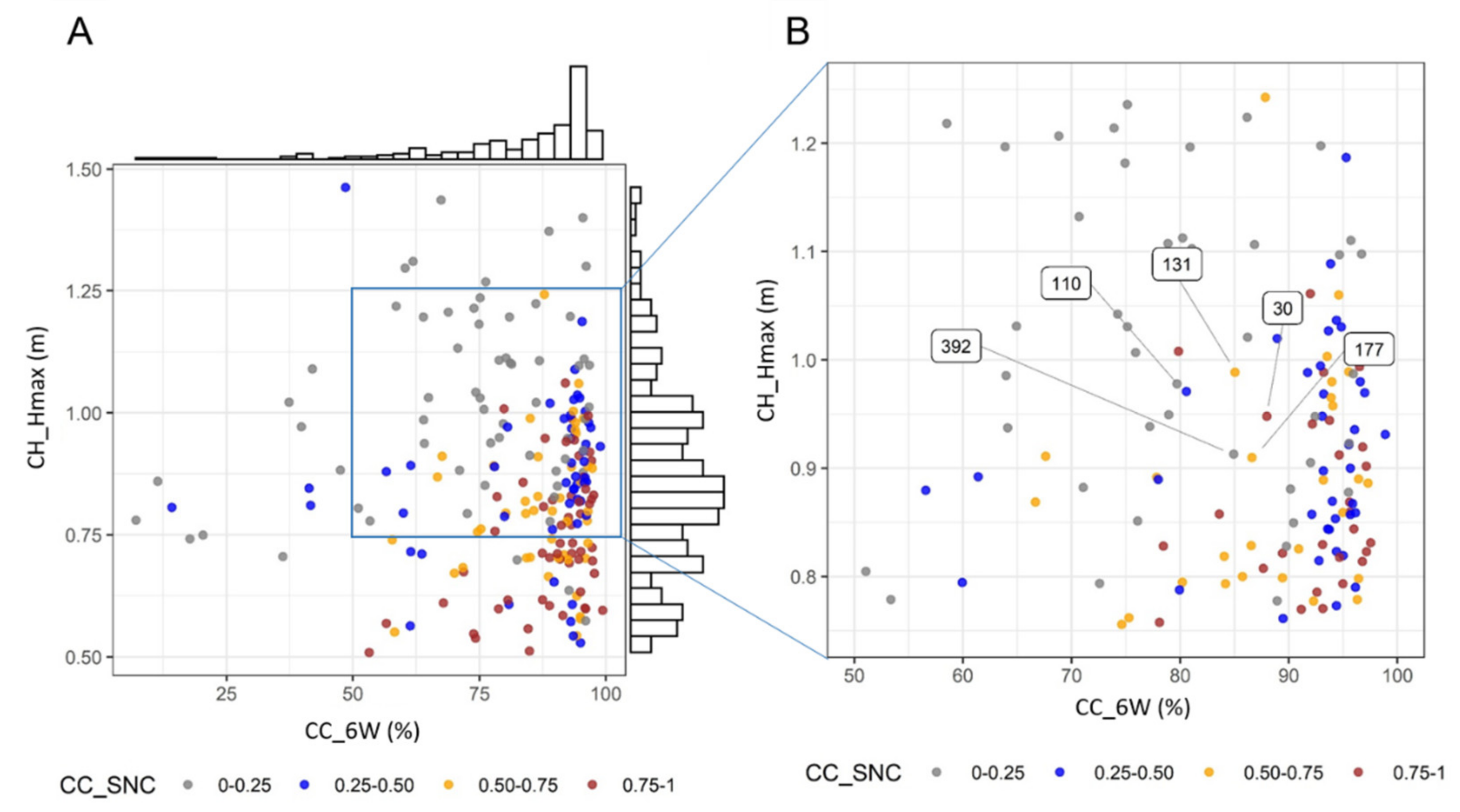
In a next step, we explored the information obtained in a breeding context to detect any plots displaying interesting traits. For example, by plotting genotypes/plots in terms of relevant complementary trait values (e.g., CH_Hmax, CC_6W and CC_SNC; maximum height reached, fast soil coverage and the rate of senescence, respectively) (Figure 9A). As apparent in Figure 9, taller genotypes have a tendency to senesce later. Based on the values obtained, breeders could select a plot with a high CC_6W (good weed suppression), not too tall (low sensitivity to lodging), not too small (strong correlation with seed yield) and a fast senescence. As indicated in Figure 9B, plot number 30 fulfils these criteria (plots 110, 131, 177, and 392 are also not too tall and display a good weed suppression, but they senesce later).

4. Discussion

4.1. General Assessment of the Methodology Developed

Weekly flights (n = 14) of a UAV equipped with an RGB sensor allowed to phenotype a large field trial during the entire growing season in terms of the dynamics of canopy cover based on the calculation of the vegetation index Excess Green (ExG), and canopy height based on the Structure from Motion (SfM) photogrammetry with high temporal and spatial resolution. These data were used to fit sigmoid curves (Gompertz and Beta function) in an automated fashion using R scripts. Model parameters to objectively describe the different soybean plots/genotypes were extracted. The methodology presented here is suitable for the efficient phenotyping of a large number of genotypes under field conditions and can provide breeders with trait information that may be difficult to obtain using other methods, e.g., maximum absolute growth rate, weed suppressive ability, onset and evolution of senescence or determinacy. Large differences were observed among the four groups considered, and high variability was present within the groups (~genotypes). The full canopy cover was reached starting from day of the year (DOY) 165 (mid-June). A decrease in cover and height was observed starting from DOY 200 (mid/end July) and was related to the onset of senescence.

By fitting a sigmoid growth function such as the Gompertz or the Beta function to multi-temporal data, it is possible to determine reliable parameters with a straightforward biological meaning enabling characterization of between-plot differences in growth and developmental processes [22]. An extra advantage of curve fitting to multi-temporal data is that possible small errors at one time point are smoothed out using the entire time series. However, model choice is critical because use of the wrong model can introduce bias [23]. The success rate reached for model fitting was 91.0% for canopy cover and 99.6% for canopy height, hence the models chosen were appropriate for fitting these data. The majority of the cases that did not reach a good fit, originated from CC data mainly from genotypes of GP1, the group first sown. Thus, a bad fit was most likely a combination of having only two data points in the increasing phase of the Gompertz model fit for CC data, the first data point having already a canopy cover of >15%, and the reduced flexibility of the Gompertz function to properly fit the first time points. These first time points are important for the model fit, as these present bigger differences because of rapid growth. This suggests that for UAV based phenotyping using time series, flights should start early enough, at plant emergence, and should last long enough to enable full senescence of all treatments. This sometimes conflicts with traditional experimental methods. In this case, bird netting was used to cover the field trial at the time of emergence to prevent bird damage. This of course interferes with UAV imaging, requiring removal and replacement of large areas of netting at the starting phase of the experiment. Near the end of the experiment, full senescence is not always required in a breeding trial before harvests are performed. Therefore, before starting the experiment, these issues should be discussed carefully between the breeders and the phenotyping researchers. A gap in the dataset can happen too—in this study, no flights were possible between July 25 and August 16. This was solved by the curve fitting, as the values during the two weeks gap were estimated. On July 25 the canopy was fully closed, and on August 16 senescence has been initiated only for some plots. Potentially, this could affect the parameters CC_SNC and CH_SNC, but not all other parameters, as full canopy and maximum height were reached before that gap. Scripting the models in R proved appropriate to automatize the fitting step for large sets of plots. Nevertheless, care should be taken to define appropriate initialization values for the Gompertz model as an optimization was not always achieved with the optimx function in R. In our case different values needed to be tested. Regarding canopy height, some datasets contained close to zero or even negative values for some plots in the first and the second flight. This can be explained by the intrinsic altimetric error and the difficulty of detecting small objects in the photogrammetry process of a flight [10]. This “noise” cannot be corrected or removed, but is in our opinion acceptable (x-y-z average error is 0.07 m).

4.2. Describing General Growth Patterns in the Different Groups

Using the derived and estimated phenotypic parameters (Figure 4; Figure 5), it was possible to detect and quantify differences among the groups. A relevant trait is the canopy cover at six weeks after emergence (CC_6W) as this is related to weed suppression capacity and row closure. In this study, most of the plots of GP3 and GP4 had CC_6W values >90% and closed the row faster than the other two groups. Senescence was also different among groups, with fast senescence for GP4. For CH_AGRmax comparable values were observed for GP3 and GP4 and for GP1 and GP2, but at different thermal times (CH_tm). By combining the results obtained for CH_Hmax and CH_te, we can conclude that plots of GP4 did not grow tall (relatively lower CH_Hmax) but grew faster (lower CH_te in combination with higher CH_AGRmax) than plots in other groups. This confirms our expectations, as GP4 comprised genotypes expected to develop quickly and mature early, according to the information available beforehand. We can thus conclude that the pipeline developed to characterize the seasonal growth and development of soybean is functional and suitable for implementation in real-time breeding applications.

Determinacy describes the extent to which a plant continues to produce extra internodes and consequently extra possibilities to produce pods and seeds after entering the generative phase (R1). Indeterminacy or semi-determinacy can be a favorable trait in soybean for cultivation in Northwest Europe as it represents an ‘insurance policy’ if a period of unfavorable weather conditions occurs, such as low temperature during flowering or drought in the summer months. Based on experience, determinate genotypes perform less well under Northwestern European conditions [24,25]. In contrast, a high level of determinacy contributes to a synchronous seed maturation, avoiding variable moisture content in the harvested seed that could cause quality problems. In soybean, determinate cultivars are used in areas with long growing seasons while indeterminate cultivars are more suited to short growing seasons [26]. Detailed information on this trait is therefore very useful for soybean breeders. Here, we present a method to estimate determinacy in a straightforward way that could be implemented routinely in soybean breeding. Overall, genotypes included in groups 1 and 2 had a higher level of indeterminacy and kept growing during a longer thermal time.

4.3. Estimating SY and Maturity Using UAV-Derived Information

In Northwest Europe, early maturity (quick progress to R8) in combination with high seed yield and a high protein content are important breeding targets. We evaluated if seed yield (SY) and the R8 stage could be predicted by an MLR with the individual time series data points or with the estimated and derived phenotypic parameters as variables. Similar adjusted R² values were obtained using the data of the different flights and using the derived phenotypic parameters. This demonstrates that the phenotypic parameters captured all variance present. Seed yield is influenced by canopy cover because a longer lasting canopy cover most likely results in more photosynthesis for optimal SY at the end of the growing season. This is supported by the presence of CC_SNC in the first MLR model and because four out of five time points included were CC data for the second model. Canopy height also plays a role in terms of growth rate and the moment when maximum height is reached. An early senescence decreases SY and the later the maximum height is reached, the higher the chances for a higher SY.

Maturity (R8) was determined by more CC time points (five dates, DOY range 164–246) than CH time points (three dates were included). The phenotypic variable CC_SNC has the most influence on R8 followed by CH_tm. Similar results related to maturity prediction classification (93% accuracy) were achieved in Yu et al. 2016 [12] using RGB and NIR drone data. In the present study we obtained similar results using higher resolution RGB imagery but by using simpler statistical methods (MLR). Soybean agronomic traits such as yield, maturity, and height were predicted in Yuan et al. (2019) [27] using six flights over four locations by color and texture features. Resulting R² values were 0.68, 0.76, and 0.27, respectively, using five regression modeling techniques, i.e., Partial Least Squares Regression, Random Forests, Cubist, Artificial Neural Networks, and Support Vector Regression. In our case, seed yield and R8 estimated by MLR achieved an adjusted R² of 0.51 and 0.85, respectively, which is slightly lower for SY but higher for maturity.

4.4. Perspectives for Practical Applications

The UAV-estimated and derived phenotypic data can be used directly in a breeding context, as they are related to relevant traits, e.g., weed suppression capacity, fast canopy establishment, early vigor, growth rates, maximum plant height, risk for lodging, determinacy, etc., for each genotype. For example, maximum plant height contributes negatively to lodging resistance, while it is positively correlated with the number of internodes, which in turn is positively correlated with the number of pods. Therefore, breeders should find a compromise considering different traits. For example, the combination of CC_6W, CH_Hmax, and CC_SNC makes it possible to identify genotypes that combine appropriate values for the different traits.

Besides the use in a breeding context, multi-temporal data can be highly valuable for plant and crop modeling. Time series of different traits have been found to be essential for proper and identifiable parameter estimation [17]. Large amounts of data can be gathered using UAV with a high temporal resolution.

4.5. Practical Lessons Learned and Future Perspectives

The high spatial resolution achieved from the UAV flights (0.5 cm pixel size for the orthophotos and 1.25 cm for the DEM) revealed the variability present within the plot and yielded a higher number of measurements in comparison to manual data-gathering. High resolution imagery does require a longer processing time, however. To reduce the processing time, a lower spatial resolution could be defined if the aim of the study does not require highly detailed information. Future research could investigate which resolution is sufficient without influencing the predictability of traits.

In this study, we considered 14 flights spread over the entire growing season at regular intervals. This time interval was short in comparison to similar studies, which included an average of only four to 10 dates (e.g., [13,16]). During data processing and interpretation, we noticed that a different flight scheme may have been more appropriate. For example, in some cases, as senescence occurred in a short period of time, it could have been appropriate to add to extra flights at the end of the growing season. Similarly, when rapid changes (e.g., fast growth) are expected, extra time points are welcome to ensure a good fit. In this regard, the date of the first flight should also be carefully chosen to capture the entire growing season. In conclusion, planning the flights according to the expected development of the crop may yield more useful data than regular intervals between flights.

5. Conclusions

In this study we collected UAV data of a soybean field trial at an unprecedented temporal resolution. The time series data allowed us to fit growth curves with high accuracy (>90%) and to derive relevant traits. The trait data that became available in this study by combining multi-temporal UAV with curve fitting will allow for a better biological interpretation of the differential response of a large set of soybean genotypes. In addition, we developed a methodology to predict seed yield and to estimate the moment at which each accession reached the R8 stage.

Furthermore, this developed strategy may be applied in the future to the analysis of multi-temporal data obtained using other sensors, e.g., multispectral, hyperspectral and thermal, to evaluate responses to abiotic and biotic stresses. This would enable the development of more resilient plant varieties at a faster pace.

References

1. Mir, R.R.; Reynolds, M.; Pinto, F.; Khan, M.A.; Bhat, M.A. High-throughput phenotyping for crop improvement in the genomics era. Plant Sci. 2019, 282, 60–72. [Google Scholar] [CrossRef] [PubMed]
2. Shakoor, N.; Lee, S.; Mockler, T.C. High throughput phenotyping to accelerate crop breeding and monitoring of diseases in the field. Curr. Opin. Plant Biol. 2017, 38, 184–192. [Google Scholar] [CrossRef] [PubMed]
3. Yang, G.; Liu, J.; Zhao, C.; Li, Z.; Huang, Y.; Yu, H.; Xu, B.; Yang, X.; Zhu, D.; Zhang, X.; et al. Unmanned Aerial Vehicle Remote Sensing for Field-Based Crop Phenotyping: Current Status and Perspectives. Front. Plant Sci. 2017, 8, 1111. [Google Scholar] [CrossRef] [PubMed]
4. Araus, J.L.; Kefauver, S.C. Breeding to adapt agriculture to climate change: Affordable phenotyping solutions. Curr. Opin. Plant Biol. 2018, 45, 237–247. [Google Scholar] [CrossRef] [PubMed]
5. Walter, A.; Liebisch, F.; Hund, A. Plant phenotyping: From bean weighing to image analysis. Plant Methods 2015, 11, 14. [Google Scholar] [CrossRef] [Green Version]
6. Yu, K.; Kirchgessner, N.; Grieder, C.; Walter, A.; Hund, A. An image analysis pipeline for automated classification of imaging light conditions and for quantification of wheat canopy cover time series in field phenotyping. Plant Methods 2017, 13, 15. [Google Scholar] [CrossRef]
7. Mullan, D.J.; Reynolds, M.P. Quantifying genetic effects of ground cover on soil water evaporation using digital imaging. Funct. Plant Biol. 2010, 37, 703. [Google Scholar] [CrossRef]
8. Sayed, M.A.; Schumann, H.; Pillen, K.; Naz, A.A.; Léon, J. AB-QTL analysis reveals new alleles associated to proline accumulation and leaf wilting under drought stress conditions in barley (Hordeum vulgare L.). BMC Genet. 2012, 13, 61. [Google Scholar] [CrossRef] [Green Version]
9. Viljanen, N.; Honkavaara, E.; Näsi, R.; Hakala, T.; Niemeläinen, O.; Kaivosoja, J. A Novel Machine Learning Method for Estimating Biomass of Grass Swards Using a Photogrammetric Canopy Height Model, Images and Vegetation Indices Captured by a Drone. Agriculture 2018, 8, 70. [Google Scholar] [CrossRef] [Green Version]
10. Borra-Serrano, I.; De Swaef, T.; Muylle, H.; Nuyttens, D.; Vangeyte, J.; Mertens, K.; Saeys, W.; Somers, B.; Roldán-Ruiz, I.; Lootens, P. Canopy height measurements and non-destructive biomass estimation of Lolium perenne swards using UAV imagery. Grass Forage Sci. 2019, 74, 356–369. [Google Scholar] [CrossRef]
11. Zhang, C.; Kovacs, J.M. The application of small unmanned aerial systems for precision agriculture: A review. Precis. Agric. 2012, 13, 693–712. [Google Scholar] [CrossRef]
12. Yu, N.; Li, L.; Schmitz, N.; Tian, L.F.; Greenberg, J.A.; Diers, B.W. Development of methods to improve soybean yield estimation and predict plant maturity with an unmanned aerial vehicle based platform. Remote Sens. Environ. 2016, 187, 91–101. [Google Scholar] [CrossRef]
13. Holman, F.H.; Riche, A.B.; Michalski, A.; Castle, M.; Wooster, M.J.; Hawkesford, M.J. High throughput field phenotyping of wheat plant height and growth rate in field plot trials using UAV based remote sensing. Remote Sens. 2016, 8, 1031. [Google Scholar] [CrossRef]
14. Pugh, N.A.; Horne, D.W.; Murray, S.C.; Carvalho, G.; Malambo, L.; Jung, J.; Chang, A.; Maeda, M.; Popescu, S.; Chu, T.; et al. Temporal Estimates of Crop Growth in Sorghum and Maize Breeding Enabled by Unmanned Aerial Systems. Tppj 2018, 1. [Google Scholar] [CrossRef]
15. Chang, A.; Jung, J.; Maeda, M.M.; Landivar, J. Crop height monitoring with digital imagery from Unmanned Aerial System (UAS). Comput. Electron. Agric. 2017, 141, 232–237. [Google Scholar] [CrossRef]
16. Han, L.; Yang, G.; Yang, H.; Xu, B.; Li, Z.; Yang, X. Clustering Field-Based Maize Phenotyping of Plant-Height Growth and Canopy Spectral Dynamics Using a UAV Remote-Sensing Approach. Front. Plant Sci. 2018, 9, 1–18. [Google Scholar] [CrossRef] [Green Version]
17. De Swaef, T.; Bellocchi, G.; Aper, J.; Lootens, P.; Roldán-Ruiz, I. Use of identifiability analysis in designing phenotyping experiments for modelling forage production and quality. J. Exp. Bot. 2019, 70, 2587–2604. [Google Scholar] [CrossRef]
18. Fehr, W.; Caviness, C. Stages of Soybean Development; Iowa State University: Aldrich Ames, IA, USA, 1977; p. 87. [Google Scholar]
19. Woebbecke, D.M.; Meyer, G.E.; Von Bargen, K.; Mortensen, D.A. Color indices for weed identification under various soil, residue, and lighting conditions. Trans. ASAE 1995, 38, 259–269. [Google Scholar] [CrossRef]
20. Zeide, B. Analysis of Growth Equations. For. Sci. 1993, 39, 594–616. [Google Scholar] [CrossRef]
21. Gompertz, B. On the nature of the function expressive of the law of human mortality, and on a new mode of determining the value of life contingencies. In a letter to Francis Baily, Esq. F. R. S. &c. Philos. Trans. R. Soc. Lond. 1825, 182, 513–583. [Google Scholar]
22. Yin, X.; Goudriaan, J.; Lantinga, E.A.; Vos, J.; Spiertz, H.J. A flexible sigmoid function of determinate growth. Ann. Bot. 2003, 91, 361–371. [Google Scholar] [CrossRef] [PubMed]
23. Thorney, J.H.M. A New Formulation of the Logistic Growth Equation and Its Application to Leaf Area Growth. Ann. Bot. 1990, 66, 309–311. [Google Scholar] [CrossRef]
24. Schori, A.; Charles, R.; Peter, D. Soja: Sélection, agronomie et production en Suisse. Rev. Suisse d’Agronomie 2003, 35, 69–75. [Google Scholar]
25. Aper, J.; De Clercq, H.; Baert, J. Agronomic characteristics of early-maturing soybean and implications for breeding in Belgium. Plant Genet. Resour. Characterisation Util. 2016, 14, 142–148. [Google Scholar] [CrossRef]
26. Ping, J.; Liu, Y.; Sun, L.; Zhao, M.; Li, Y.; She, M.; Sui, Y.; Lin, F.; Liu, X.; Tang, Z.; et al. Dt2 is a gain-of-function MADS-domain factor gene that specifies semideterminacy in soybean. Plant Cell 2014, 26, 2831–2842. [Google Scholar] [CrossRef] [Green Version]
27. Yuan, W.; Wijewardane, N.K.; Jenkins, S.; Bai, G.; Ge, Y.; Graef, G.L. Early Prediction of Soybean Traits through Color and Texture Features of Canopy RGB Imagery. Sci. Rep. 2019, 9, 1–18. [Google Scholar] [CrossRef] [Green Version]
Figure 1. Schematic overview of (a) the trial with group locations (white boxes, GP1-4), (b) zoom of two plots, marked by a red box in A, with the mask applied to the images to select pixels corresponding to vegetation, (c) timeline of the sowing dates (per GP) and UAV flights and (d) workflow followed in the manuscript.
Remotesensing 12 01644 g001
Figure 2. Schematic representation of the phenotypic parameters derived from the curve fitting for (a) canopy cover using the Gompertz function and (b) canopy height using the Beta function. For abbreviations and explanations of the parameters, see Table 1.
Remotesensing 12 01644 g002
Figure 3. Adjusted R2 of the curve fitting for canopy cover (CC_RsqA) and canopy height (CH_RsqA) data of all plots. A color code is used to show the percentage of emergence. Zoom of the plot distribution with an adjusted R2 higher than 0.70 (n = 291 plots remaining for further analysis) is included.
Remotesensing 12 01644 g003
Figure 4. Boxplots of the phenotypic parameters (af) derived from the curve fitting of canopy cover data. The data is presented per group (GP 1–4) and all groups together (All). For abbreviations see Table 1.
Remotesensing 12 01644 g004
Figure 5. Notched boxplots of the phenotypic parameters (af) derived from the curve fitting of canopy height data. The data is presented per group (GP 1–4) and all groups together (All). For abbreviations see Table 1.
Remotesensing 12 01644 g005
Figure 6. PCA of (a) UAV derived phenotypic parameters and field observations (in red) and (b) individual plots (n = 148) with color code related to the group/sowing date. For the abbreviations, see Table 1.
Remotesensing 12 01644 g006
Figure 7. Correlograms between the UAV derived phenotypic parameters and field observations per group (ad, GP1-4) and grouped (e) (n = 148). For the abbreviations, see Table 1.
Remotesensing 12 01644 g007
Figure 8. MLR model building overview for SY with RMSE and Adj. R2 evolution (a). The red dashed line indicates the selected (best) model with the lowest RMSE. The subset selection regression with normalized UAV phenotypic variables included a 10 k-fold cross validation. In each subsequent step one variable was added, and all possible combinations were evaluated. The model index = 0 included only the groups (GP1-4, GP1 is the reference group) as dummy variables. For the abbreviations, see Table 1. Graphs are provided per variable with the value of their respective coefficients (b).
Remotesensing 12 01644 g008
Figure 9. Representation of how data could be used to select interesting plots in a breeding program based on phenotypic data using three parameters: CC_6W, CH_Hmax, and CC_SNC (a). Zoom of the plot distribution based on a applicable values range for selection (b). For the abbreviations, see Table 1.
Remotesensing 12 01644 g009