ROSACE: A Proposed European Design for the Copernicus Ocean Colour System Vicarious Calibration Infrastructure

Abstract

The European Copernicus programme ensures long-term delivery of high-quality, global satellite ocean colour radiometry (OCR) observations from its Sentinel-3 (S3) satellite series carrying the ocean and land colour instrument (OLCI). In particular, the S3/OLCI provides marine water leaving reflectance and derived products to the Copernicus marine environment monitoring service, CMEMS, for which data quality is of paramount importance. This is why OCR system vicarious calibration (OC-SVC), which allows uncertainties of these products to stay within required specifications, is crucial. The European organisation for the exploitation of meteorological satellites (EUMETSAT) operates the S3/OLCI marine ground segment, and envisions having an SVC infrastructure deployed and operated for the long-term. This paper describes a design for such an SVC infrastructure, named radiometry for ocean colour satellites calibration and community engagement (ROSACE), which has been submitted to Copernicus by a consortium made of three European research institutions, a National Metrology Institute, and two small- to medium-sized enterprises (SMEs). ROSACE proposes a 2-site infrastructure deployed in the Eastern and Western Mediterranean Seas, capable of delivering up to about 80 high quality matchups per year for OC-SVC of the S3/OLCI missions.

1. Introduction

As of 2020, a number of low-earth-orbit satellites together provide systematic coverage of ocean colour radiometry (OCR) observations over the world’s oceans and coastal zones. Two programmes among this constellation are operational, which means that they are expected to maintain delivery of their observations and products over the long-term, in order to sustain a variety of uses, from, e.g., science of the long-term, climate-driven trends of the marine ecosystem, to services to government and industry users, e.g., water quality monitoring. These two programmes are the joint polar satellite system (JPSS) of the US National Oceanographic and Atmospheric Administration (NOAA), and the European Copernicus programme. The JPSS satellites carry the visible infrared imaging radiometer suite (VIIRS), delivering OCR observations in eight spectral bands in the visible and near infrared (VisNIR) spectral region. The Copernicus Sentinel-3 (S3) satellites carry the ocean and land colour instrument (OLCI), delivering OCR observations in twenty spectral bands in the VisNIR.

For these and any other OCR missions to deliver products of the desired accuracy, a system vicarious calibration (SVC) programme has to run over their entire lifetime [1], which is also a requirement for other types of Earth observation missions that intend to address climate change related questions [2]. Ocean colour SVC (OC-SVC) consists of adjusting the prelaunch mission spectral calibration coefficients of the onboard radiometers through comparison of the top-of-atmosphere (TOA) radiance measured by the mission, to the same quantity derived from using high-quality radiometry data collected in the field and radiative transfer computations to propagate the bottom-of-atmosphere field measurements to TOA [3]. SVC therefore requires a sustained post-launch field programme to collect the necessary data, with the aim of maintaining the level of uncertainty of the derived satellite products within predefined requirements [4,5,6,7]. This need for SVC has been demonstrated since the early times of the satellite OCR era [8]. Modern satellite OCR observations must indeed provide the water-leaving radiance in the blue part of the electromagnetic spectrum with a < 5% accuracy over meso- to oligotrophic waters [9,10], which translates as an uncertainty of about 0.002 in reflectance at 443 nm [11] when reflectance is modelled from chlorophyll following [12]. Since the marine signal is generally < 10% of the TOA radiance measured by the spaceborne sensor, achieving this goal requires that the instruments be calibrated to better than 1% uncertainty. This cannot be reached using only onboard calibration devices such as sun diffusers, hence the need for OC-SVC. It is worth remembering that OC-SVC is not an absolute calibration of the sensor. It is an adjustment of the overall response of the sensor plus the atmospheric correction algorithm [1,8]. The goal is to absorb residual uncertainties in order to obtain final products, e.g., the normalized water-leaving reflectance or radiance with the desired accuracy.

Until now, two field programmes have provided space agencies with OC-SVC-quality field observations, both using a moored optical buoy. The marine optical buoy (MOBY [13,14]) has been in operation since 1995 off the island of Lanaï in the Hawaiian archipelago. It continuously delivers hyperspectral reflectance for SVC of the NASA and NOAA instruments (sea-viewing wide field-of-view sensor, SeaWiFS, moderate resolution imaging spectroradiometer, MODIS and VIIRS), and has also been used by international missions, e.g., the European Space Agency (ESA) medium resolution imaging spectrometer (ENVISAT/MERIS), and the Japan Aerospace Exploration Agency (JAXA) global change observation mission-climate, second generation global imager (GCOM-C/SGLI). Another SVC programme was set up to support European OCR missions, at that time the ESA ENVISAT/MERIS. This programme is named BOUSSOLE (“BOUée pour l’acquiSition d’une Série Optique à Long termE” [15,16]) and has been operating continuously since 2003 at an open ocean site in the Northwestern Mediterranean Sea. It is currently used for SVC of the Copernicus Sentinel-3A and -3B OLCI instruments and for the GCOM-C/SGLI. Data from both programmes have also been used for the SVC of satellite sensors not specifically designed for ocean colour applications such as the thematic mapper (TM) on Landsat 5 and 7, the operational land imager (OLI) on Landsat 8, and the multispectral instrument (MSI) on Sentinel-2A&B [17,18,19].

The European Organisation for the Exploitation of Meteorological Satellites (EUMETSAT) is in charge of the S3/OLCI marine ground segment as part of Copernicus operations. As such, they envision having a fully independent European in situ OC-SVC infrastructure deployed and operated for the long-term, as has been recommended for the support of Copernicus ocean colour missions [20]. In order to properly set up this significant investment, they first commissioned a study in 2017 to summarize requirements for such an infrastructure [21]. They then called for ideas for what this European OC-SVC infrastructure could be through an invitation to tender (ITT) in 2018, from which they commissioned two studies that worked in parallel during 2019 and delivered their proposed preliminary designs by December of the same year.

This paper summarises the main characteristics of one of the proposed OC-SVC infrastructures, named ROSACE, which stands for “Radiometry for Ocean colour Satellites Calibration and community Engagement”. The high-level rationale for the proposed solution is presented first. The characteristics of the two sites that compose the field segment are then detailed along with the deployment platform, followed by the overall strategy and equipment for the optical system and its calibration. The methodology used to assess the preliminary uncertainty budget of the proposed system is then summarised and results presented. Finally the organisation of the ground segment and the infrastructure operations are outlined. In addition, an autonomous platform capable of hosting the optical system is presented as an option to improve the overall capacity of the infrastructure.

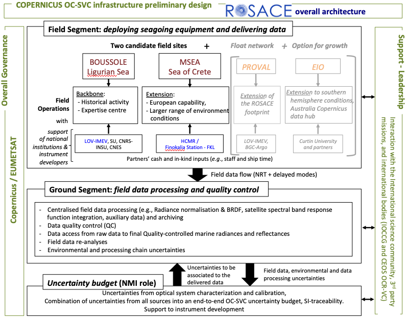
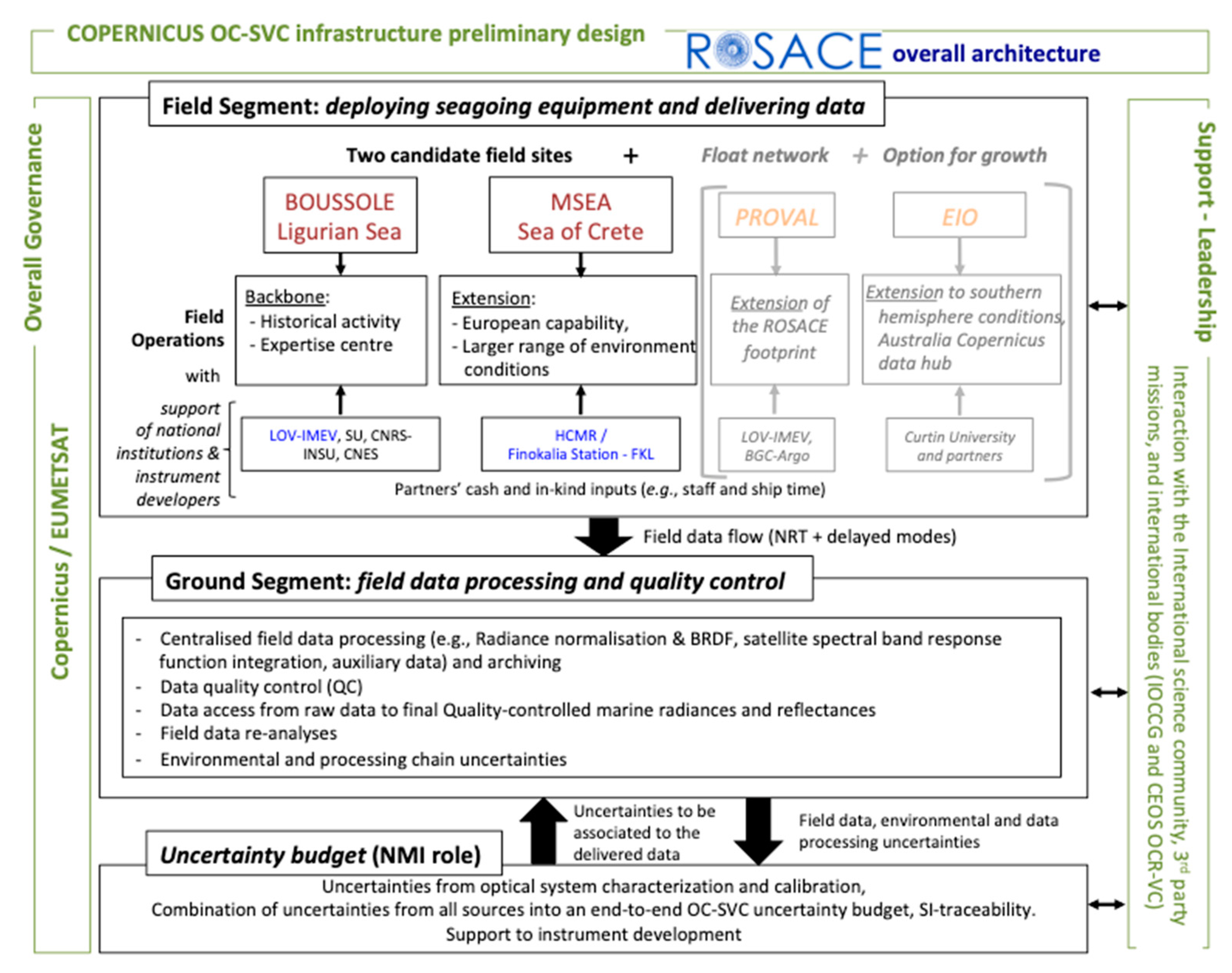
2. High-Level Rationale for the Proposed ROSACE OC-SVC Infrastructure

The high-level rationale underlying the ROSACE preliminary design (Figure 1) is to:

• Take advantage as much as possible of existing European expertise in OC-SVC that has been developed in the past two decades under European (ESA in particular) and national funding, including field operations, SI-traceability and evaluation of uncertainties, associated data quality assurance and quality control and processing and generation of satellite matchups and OC-SVC gains.
• Reinforce the above and, in addition, build a new European capability in the domain of OC-SVC field radiometry, in order to ensure long-term sovereignty and stability of the Copernicus SVC infrastructure. This includes two sites, collaboration with a national metrology institute (NMI), and new technology developments. The two field sites are in the Ligurian Sea (BOUSSOLE heritage) and the Cretan Sea (MSEA). They were selected by the ESA “Fiducial Reference Measurements For Satellite Ocean Colour” (FRM4SOC [22,23]) study as the two of the best European locations among those currently under evaluation, in part because significant logistical capabilities adapted to maintaining an OC-SVC infrastructure already exist at these sites.
• Rely on strong national support in conjunction with the main Copernicus funding to ensure that the ROSACE OC-SVC infrastructure is backed by long-term sustainable staff, capability and logistical resources.
• Be ready to incorporate additional partnerships in order to improve redundancy inside the OC-SVC infrastructure, to enlarge the database onto which the uncertainty budget is built, to improve, if needed, the methodological baseline used to compute the SVC gains, and to increase the matchup capacity of the OC-SVC infrastructure.

In this logic, collaboration with a possible third site in the Eastern Indian Ocean (EIO, off Western Australia) is envisaged, which has also been identified by the FRM4SOC study (see also [24]). This is an option for future extension of the infrastructure, only possible if the EIO site would have the technical capability. Additionally, included in the preliminary design is the possibility to increase the capacity of the infrastructure to deliver in situ data by deploying autonomous profiling floats [25].

5.

Ensure close communication with international bodies that work on establishing OC-SVC requirements and fostering international collaboration (e.g., the International Ocean Colour Coordinating Group, IOCCG and the Committee on Earth Observation Satellites Ocean Colour Virtual Constellation, CEOS OCR-VC).

6.

Maintain development activities that are vital to allow improvement in data acquisition and processing procedures and ultimately improve the data quality of the OC-SVC infrastructure, and also to better secure national support for this European infrastructure.

The rationale supporting ROSACE is rather simple. It consists of leveraging the two-decade-long experience as well as previous European investments in order to be in a position to deliver an operational system meeting the Copernicus requirements in the time frame anticipated by EUMETSAT, i.e., likely in line with the launch of the Sentinel-3 C and D units and beyond (from 2023/2024).

That is why ROSACE capitalises on the single existing European OC-SVC infrastructure, i.e., the BOUSSOLE site and project, as the backbone that supports the development of a more European-integrated system, including a second European site in the best suited location of the European Seas for OC-SVC, i.e., the MSEA site. This strategy appears as the most robust approach to achieve, in a safely managed way, the full compliance with the stringent requirements of an operational programme like Copernicus/Sentinels, including lowering the uncertainties in OC-SVC.

ROSACE also incorporates innovative solutions, in the development of specifically designed European instruments and calibration devices that will fully match the OC-SVC requirements and fulfils the need for modularity, and the possibility to integrate a network of autonomous profiling floats to complement the fixed sites.

The success of such a long-term service for the Copernicus programme also depends on adequate competence transfers and periodic training. This is one of the roles assigned to universities and public research institutions involved in ROSACE, i.e., to transfer knowledge, and it constitutes a fundamental task for building a long-term infrastructure that will operate across generations.

3. The Field Segment

3.1. Metrology Rationale

At the present time, SVC is the only means to achieve the uncertainties needed for remotely sensed OCR observations. It is well established that the SVC reference system (radiometry measurements) needs to be robustly tied to the International System of Units (SI) and be collected in meso- to oligotrophic waters, ideally from a location with stable oceanographic conditions [6,8]. Provided that there are enough reliable observations of the site from space for any given sensor to allow statistically reliable calibration, it could be argued that the SVC requirements can be achieved by a single infrastructure, in a single location. This would also require that the instrumentation, maintenance and recalibration, is unequivocal and guaranteed to be operational in this manner for the foreseeable future. In the case of climate monitoring and the Copernicus series of sensors this timescale must span many decades. This guarantee must stand irrespective of funding and unexpected events, either natural or manmade. The 2020 global pandemic [26] is an example where large numbers of assets had to be recovered from sea because their servicing or emergency recovery were no longer feasible during lockdown measures taken by many governments (e.g., [27]). Equipment or site redundancy and autonomous platforms can help in such circumstances.

It soon becomes clear that implementation of a single site infrastructure is of high risk and in engineering terms considered a single critical point of failure. Even if multiple spares are ready and waiting to be deployed, a single (non-independently checked) calibration route provides a risk that no metrology institute would safely rely upon for any measurement. Primary radiometric scales and ancillary measurements are regularly checked across international borders through formal comparison with peers to ensure consistency and avoidance of any potential errors, (standards/procedures/typographical). This comparison process is a fundamental requirement to ensure international consistency of measurements and trade.

It thus becomes apparent that a minimum requirement to ensure long term consistency and reliability of a reference measurement system for OC-SVC is two independently calibrated systems of similar performance and in different geographical locations. It is also clear that providing the two independent measurement systems always agree (within their uncertainties) then this strategy of two measurement systems can probably be relied upon. However, as anyone making comparative measurements knows, if the two references disagree then you are left with the question of which one do you believe?

For this reason it is normal practise, for any reference, e.g., a standard light source (FEL lamp) or detector, to consist of a group of a minimum of three entities, to provide redundancy and the likelihood of at least two being consistent and a probabilistic indicator of closeness to the truth. The recent redefinition of the kilogram for example was only considered reliable and acceptable once there were three independent measurements made that were consistent within their uncertainties (also below a prescribed minimum level) and that at least two of the measurements had to be from a completely different traceability route. A robust long-term reference for OC-SVC should follow the same minimal metrological rigour, i.e., at least three independent measurement infrastructures and at least two independent traceability paths. The ROSACE proposal of two linked European sites, when added to the existing North American MOBY infrastructure, meets both these metrological requirements.

There are many other benefits, such as a redundancy from unforeseen system failures, increased number of matchup opportunities, randomisation of environmental effects, etc. but fundamentally, a global system of just two sites would be metrologically and operationally high risk. Following the same metrological rationale, ROSACE will allow “built in” systematic round robin intercalibration exercises to validate (1) the calibration procedures between the two field sites and a third independent calibration system operated by the Tartu Observatory and (2) the consistency of measurements and uncertainties between the two sites with an independent transfer profiling radiometer (see also Section 7.1).

3.2. Practical Considerations, Specific Role of Each Site

Other elements, of a more practical type, have also been considered in selecting two sites to develop the ROSACE OC-SVC infrastructure. Essentially, what we proposed was not a simple doubling of identical (twin) sites. It rather takes advantage of specific aspects present at the two locations in order to leverage their complementarity. These elements are:

• Geophysical properties are similar yet different enough at the two sites, so that they are complementary, not simply redundant (see the sites descriptions in Section 3.3 and Section 3.4).
• Expertise in deploying and maintaining large oceanographic buoys is similar at the two sites, i.e., the Laboratoire d’Océanographie de Villefranche from the Institut de la Mer de Villefranche (LOV-IMEV) and the Hellenic Centre for Marine Research (HCMR). However, a longer and more developed experience with optics, radiometry and OC-SVC exists at LOV-IMEV.
• BOUSSOLE buoys and instrumentation exist at LOV-IMEV, ready to be used (until improved versions become available) in continuation of the present effort and to host the new optical system for testing, and ensure continuity of the time series.

Therefore, the logic is to use the BOUSSOLE site not only for operational delivery of OC-SVC data, which certainly remains a main objective, but also as a development and test site, where:

• Improvements in the buoy structure can be tested before new versions are built and operationally deployed at MSEA and BOUSSOLE.
• The new optical system can be deployed in parallel to the one currently used (SeaBird HyperOCR radiometers). This is not to qualify the new radiometer system, which will be of superior radiometric quality to that of the current one, but rather is an opportunity to ensure continuity of the time series between MERIS and OLCI observations.
• Testing of new equipment or further improvement of the optical system, can be carried out on one site before being transitioned to permanent upgrades at both sites.

3.3. The BOUSSOLE Site

3.3.1. Location and General Characteristics

The BOUSSOLE site is located at 32 nmi (59 km) offshore from Nice (France) in the NW Mediterranean Sea (43°22′ N, 7°54′ E; Figure 2). Water depth at the site is about 2440 m. This site has been already described in detail in [28], which readers are referred to. Here we provide a summary of the features that are most relevant to OC-SVC. Time series, histograms and climatological values of a number of parameters can be found in [29].

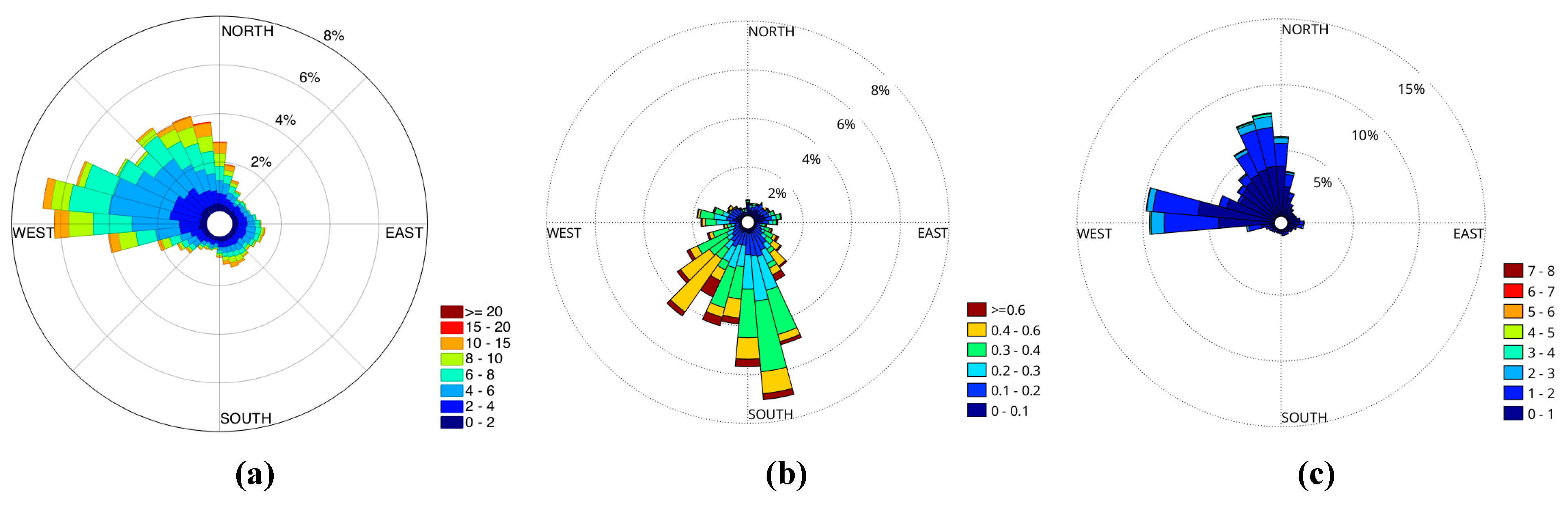
3.3.2. Weather and General Hydrology

Wind speeds at BOUSSOLE are generally moderate (Figure 3a). Over the past 15 years, only 3% of recorded wind speeds were greater than 15 m s⁻¹, and 16% of records were above 10 m s⁻¹. These higher wind speeds, and the associated larger waves are concentrated in the 5 months from November to March. Dominant wind directions are from the west to southwest and from the northeast sectors (Figure 3b). These are channelled into these two main directions on the one hand by the general atmospheric circulation of the region, and, on the other hand, by the topography formed by the Alps and Corsica.

Significant wave heights at BOUSSOLE were mostly less than 2 m, although values as high as 5 m could be occasionally recorded (Figure 3c). The wave period (not shown) was around 4–6 s, which is typical of the Mediterranean Sea.

This site was selected in particular because currents are extremely low. This peculiarity is due to the position close to the centre of the cyclonic circulation that characterizes the Ligurian Sea. The northern branch of this circulation is the Ligurian current, forming a jet flowing close to the shore in the NE to SW direction and creating a front whose position is seasonally varying, closer to the shore in winter than in summer. The southern branch is a SW to NE current flowing north of Corsica and the eastern part of the circulation is simply imposed by the geometry of the basin. The 17 years of BOUSSOLE deployments have confirmed the low-current character of the site (high currents would have been identified as strong buoy tilts). Stronger currents have been very occasionally revealed through observing the buoy plunging unusually deep. This situation occurred only four times during the 17 years of deployment and, for each instance, the event lasted generally less than a day.

The temperature and salinity conditions at BOUSSOLE are illustrated in Figure 4a. The minimum sea surface temperature (SST) was about 12.7 °C (associated with a salinity of 38.4 psu), which is a constant value reached in the coldest winters when the water mass was fully mixed down to the bottom. This deep mixing contributed to the formation of the bottom waters of the Western Mediterranean Sea.

3.3.3. Phytoplankton Chlorophyll-a, Water Type and Inherent Optical Properties

The seasonality of the physical forcing drove the seasonal changes of nutrients and phytoplankton, as illustrated here by the surface nitrate and total chlorophyll-a concentrations ([TChl-a], Figure 4b). Oligotrophic conditions prevailed during the summer with undetectable nitrate levels and [TChl-a] lower than 0.1 mg m⁻³ (with a minima around 0.05 mg m⁻³). The higher concentrations are on average in the range 0.8-1.7 mg m⁻³ (with a maxima up to about 5 mg m⁻³), during the early spring bloom (February to March or April) when surface waters are nitrate replete. Moderate [TChl-a], between 0.1 and 0.2 mg m⁻³, characterize most of the other periods of the year. Interannual variability of physical forcing, specifically the depth of the winter convection, determines the magnitude of the phytoplankton spring bloom [30].

An important consequence of the above characteristics, in particular water depth, circulation, and distance from shore, is that waters at the BOUSSOLE site are permanently of the Case-1 category (following [31]). This assertion is quantitatively evaluated by plotting the irradiance reflectance at 560 nm, determined from the buoy measurements, as a function of [TChl-a] (Figure 5), and superimposing on top of the data a theoretical upper limit of this reflectance for Case-1 waters [32]. With the exception of a few outliers, all data points are below the curve, demonstrating that waters permanently belong to the Case-1 type at the BOUSSOLE site.

Inherent optical properties (IOPs) measured at the BOUSSOLE site include the particulate absorption coefficient (a_p, from samples collected during monthly cruises), the particulate backscattering coefficient, b_bp, and the particulate beam attenuation coefficient, c_p. Average seasonal cycles are displayed in Figure 6. These parameters also clearly illustrate the seasonal variability at BOUSSOLE, consistent with the description already provided for [TChl-a]. This is expected for typical Case-1 waters.

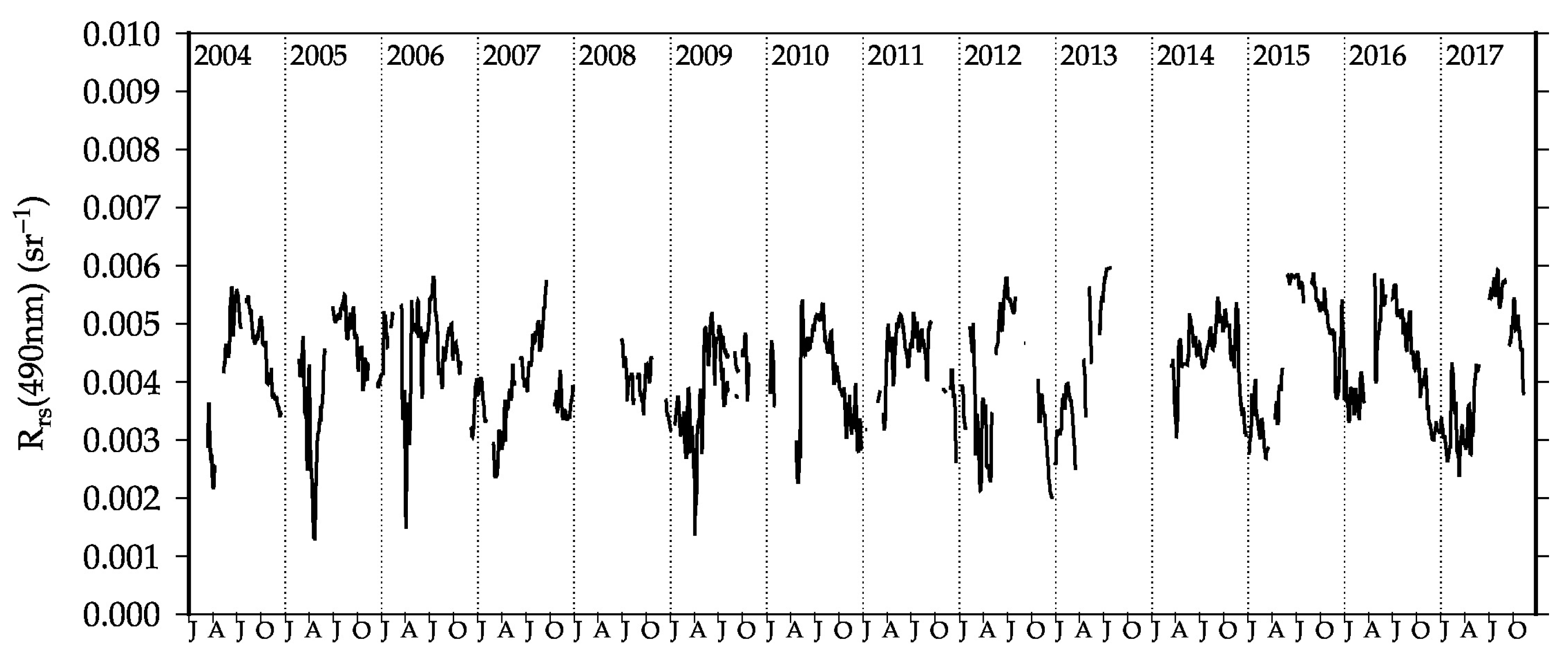
3.3.4. Remote-Sensing Reflectance

Underwater downward and upward irradiances, upwelling nadir radiances and above-water downward irradiances have been measured continuously at BOUSSOLE since September 2003, initially with 7-band multispectral radiometers (Satlantic 200-series; wavelengths 412, 443, 490, 510, 560, 670 and 683 nm) and, from 2007, also using hyperspectral radiometers (Satlantic HyperOCR series; 350–850 nm with a 3 nm resolution). The multispectral instruments have been decommissioned at the end of 2017.

Apparent optical properties (AOPs) are derived from these measurements, such as the diffuse attenuation coefficient for downward irradiance or the remote sensing reflectance [16,28]. The latter is shown in Figure 7, for λ = 443 nm, as an example illustrating the seasonal signal as well as the quasi-systematic observations through the 14 years displayed here.

3.3.5. Atmospheric Parameters

BOUSSOLE benefits from the general conditions prevailing in the Mediterranean Sea, which is known for being a rather clear-sky area. Seasonal cycles derived from the MODIS cloud fraction products are displayed in Figure 8a and they clearly illustrate these characteristics.

The aerosol optical depth (AOD) and aerosol Angstrom exponent have been derived both from measurements at a coastal AERONET site (Cap Ferrat; 43°41′ N, 7°20′ E; automatic CIMEL CE318 sun photometer) and from measurements at the BOUSSOLE site offshore, using a hand-held CIMEL CE317 sun photometer. These measurements reveal that AODs are actually extremely similar at both sites (Figure 8b), with seasonal values from around 0.05 to 0.1 at 865 nm. The Angstrom exponents, which are determined by the aerosol types and their size distribution, are however markedly different, with values steadily around 1.4 at the Cap Ferrat station and around 0.6 at the BOUSSOLE site. This is also expected, because coastal aerosols include a larger proportion of small particles of continental origin than marine aerosols, and therefore have a larger Angstrom exponent.

The total ozone content over BOUSSOLE varied from about 290 to 400 Dobson units (DU, not shown), with maxima generally in winter and minima at the end of summer. Average values in summer were around 340 DU. These values were derived from data of the NASA AIRS (Atmospheric Infrared Sounder), also indicating a decline of concentrations since around 2011.

3.3.6. Spatial Homogeneity

In situ measurements have a horizontal sampling scale on the order of tens of metres, whereas satellite-derived quantities have sampling scales of hundreds of metres to 1 km. Therefore, when comparing parameters derived from both approaches, an important aspect to consider is the spatial homogeneity of the measurement site.

Spatial surveys have, therefore, been conducted during BOUSSOLE monthly cruises [34], by following a grid pattern of about one square nautical mile centred on the buoy site, during which along-track fluorescence measurements were performed. Changes of this small-scale spatial variability of the chlorophyll-a fluorescence are illustrated in Figure 9 (see also Figure 4 in [28]). They show that the variability is, as expected, low during the oligotrophic summer (around ±10%). The horizontal gradients can reach larger values during the spring bloom and during fall, with values from −70% to +35% (not shown).

A ±10% change of chlorophyll when chlorophyll was initially 0.1 mg m-3 (oligotrophic conditions at BOUSSOLE) translates into changes in reflectance at 443 nm of the order of 0.0015 (3.5%).

3.3.7. Summary of the BOUSSOLE Site Characteristics Relevant to OC-SVC

The above sections have shown that BOUSSOLE is a fully characterised site in all aspects that are needed to define relevance for OC-SVC. Extremely few examples such as this exist globally, where hydrology, IOPs, AOPs, biogeochemical quantities (e.g., [TChl-a]) and atmospheric properties have been continuously sampled for nearly two decades.

The site’s main geophysical characteristics are:

• Low currents.
• Moderate wind speed/wave height.
• Case-1 waters throughout the year.
• [TChl-a] concentration < 0.1–0.2 mg m⁻³ in summer and fall.
• Characterised kilometre-scale spatial variability.
• High occurrence of clear skies.
• Low atmospheric aerosol load throughout the year.

As for the logistics:

• Well-established oceanographic institute (>130 years) close to the site (LOV-IMEV, Villefranche-sur-Mer, France).
• Well-established expertise in marine optics (>60 years).
• Well-trained permanent staff.
• Ships and other necessary equipment all available.
• Proven capacity to manage the BOUSSOLE platform.
• Proven record (>16 years) of uninterrupted acquisition of OC-SVC-quality observations.
• Field site identified on marine charts within an area identified for scientific work.
• Meteorological buoy managed by the French weather forecast agency 2 nmi from BOUSSOLE.

3.4. The MSEA Site

3.4.1. Location and General Characteristics

The MSEA site (Cretan Passage, South Sea of Crete; Figure 10) has been suggested by the global evaluation work of Zibordi and Melin [24], Zibordi et al. [20] and the FRM4SOC international OC-SVC workshop report [22] as the best region in the European Seas for OC-SVC. A more detailed analysis of available in situ oceanographic, optical, atmospheric and satellite data demonstrated very similar conditions in the Cretan Sea (north of Crete Island) and that a field infrastructure meeting the requirements for Copernicus OC-SVC can be deployed there.

When combined with logistical considerations, the best site in the Cretan Sea is in the vicinity of the HCMR operational physical and biogeochemical monitoring buoy (E1-M3A) [35]. This location, referred to as MSEA similarly to [24], is at 35°44′ N, 25°20′ E approximately 26 nmi (48 km) north of the HCMR headquarters in Crete. Specifically, it is 10 nmi east of the E1-M3A buoy to optimize the position with respect to Sentinel-3A and B overpasses.

The site has open ocean characteristics representative of a wider area of the Eastern Mediterranean [36], and a water depth of 1400–1500 m. HCMR has operated the E1-M3A buoy in this locale for over 20 years within the framework of the Monitoring, Forecasting and Information System for the Greek Seas (POSEIDON) network [37] and as part of the European contribution to the global ocean observing system (GOOS) ocean sites operational network [38]. From this buoy, a vast array of oceanographic and biogeochemical data has been, and continues to be, gathered for the area. Augmenting the data from the buoy itself are monthly sampling site visits, FerryBox data from the Athens-Crete ferry that passes to the west of the buoy, multiple deployment Argo profiler data of the local area and data from an AUV/glider that is autonomously and continuously operating on transects past the buoy [35].

The proximity of the 6000 m² HCMR-Crete research centre to the buoy provides the extensive support facilities, in terms of laboratories, human resources and research vessel support (62 m R/V Aegaeo; 24m R/V Philia), that are necessary for OC-SVC buoy operations. Furthermore, the waters surrounding the island of Crete, in the Eastern Mediterranean, are characterized by very low suspended particle concentrations, and correspond to a “no bloom” trophic regime according to [39]. The Eastern Mediterranean, including the Cretan Sea, is generally characterized by oligotrophy throughout the year making it very similar in this respect to the MOBY site near Hawaii [14]. The following sections further detail the site’s characteristics that support its prime suitability for Copernicus OC-SVC.

3.4.2. Weather and General Hydrology

In general, weather and circulation conditions at the MSEA site were calm and stable with very few extremes. Wind speeds at MSEA were generally lower and varied less than at the BOUSSOLE site. Over the 11-year period analysed (2007–2018) very few days were recorded with an established wind speed above 15 m s⁻¹. The average wind speed at the site was only 5.3 m s⁻¹ and the majority were within the range 2–8 m s⁻¹. High wind speeds (> 15 m s⁻¹) and the associated large swells were rare and might occur in the winter season from November to February. Dominant winds were from the W–NW (Figure 11a), and were channelled into this main direction by the general atmospheric circulation of the region. The Meltemi/Etesian N or NW winds are a repeating summer event for the Cretan Sea, occurring mainly in August. They are rarely very intense and average around 6 m s⁻¹. Air temperature and pressure 11 year averages were 20.09 °C (min. 2 °C; max. 32 °C; standard deviation (SD) 4.63 °C) and 1015.20 hPa (min. 995 hPa; max. 1035 hPa; SD 5.73 hPa).

Surface current data were collected from the MSEA site using an acoustic Doppler current profiler (ADCP) installed at 1 m over the last 11 years. The currents were extremely low, i.e., in the entire Cretan Sea the flows away from the coast were on the order of 0.1–0.3 m ⁻¹, in contrast to the Levantine Basin, where the meso-scale circulation structures at the near-surface layers were characterized by higher velocities reaching 0.4–0.5 m ⁻¹ [40]. Thus the majority of the currents at the MSEA site were of this low order with a measured average over the last 11 years of 0.23 m ⁻¹. The dominant currents were from the NNW towards the SSE (Figure 11b) and this was dependent on the position of the semi-permanent slow-moving anticyclonic circulation feature in the Cretan Sea [41].

Wave direction generally follows the prevailing wind direction with a slight offset further west and further north. Significant wave heights also followed the wind strength of the area with nearly all waves under 3 m since 2007 and on average less than 1 m (Figure 11c). High swell and high waves (4–7 m) were extremely rare and occurred sporadically in the winter season from November to February. The wave period for the majority of the 11 years analysed falls within the range of 2–6 s with an average of 3.96 s.

Average surface water temperature and salinity levels at the MSEA site were 21.35 °C and 39.23 psu respectively. The minimum surface temperature was 15 °C (associated with a salinity of 38.6 psu), which was a constant value reached in winter when the water mass was fully mixed down to the bottom. This deep mixing contributes to the formation of the bottom waters of the Eastern Mediterranean Sea. During summer the maximum surface temperature was 29 °C (associated with a salinity of 39.65 psu). Assimilation of these data together with Ferrybox and glider measurements around MSEA into the POSEIDON models have also allowed a better description of the hydrodynamics of the site and the wider southern Aegean area [42].

3.4.3. Phytoplankton Chlorophyll-a, Water Type and Inherent Optical Properties

In the Cretan Sea, low concentration [TChl-a] maxima tended to occur during late winter to early spring, i.e., late February to March, associated with a very limited phytoplankton spring “bloom”. Monthly in situ sampling of essential biogeochemical variables since 2010 and the deployment of a sediment trap at the site contribute to the study of ecosystem functioning and carbon export potential at MSEA [35].

Phytoplankton surface values of [TChl-a] in the offshore Cretan Sea waters varied between <0.05 and 0.2 mg m⁻³, during the stratified and mixing periods, with values < 0.1 mg m⁻³ being dominant throughout the year. Subsurface maxima (around 20 m) may rarely reach 1 mg m⁻³ during the spring bloom while deep chlorophyll maxima (below 75 m) are consistently formed for most of the year [43] and annual primary production values yield < 25 g C m⁻² [44]. This very low level of surface chlorophyll was confirmed through the analysis of bottle samples collected from the location of the MSEA site since the end of 2012. The HPLC data were considered the most accurate and the triangles in Figure 12 confirmed that chlorophyll concentrations rarely rose above 0.2 mg m⁻³ and values < 0.1 mg m⁻³ dominate.

Based on productivity and light attenuation data, Ignatiades [44] found that the waters of the Cretan Sea have a deep blue colour and an average value of the spectral attenuation coefficient (K_d), at 480 nm, of 0.040 m⁻¹. During the EU-funded CINCS project (Pelagic-Benthic Coupling in the oligotrophic Cretan Sea), five oceanographic cruises were conducted in the central Cretan Sea, focusing on the marine sector from the coast off Heraklion and up to 1700 m depth. Transmissometry profiles (at 660 nm) and bottle data from these revealed the presence of very faint nepheloid layers and very low suspended particulate matter concentrations (SPM <1.5 mg m⁻³) [45].

In terms of hyperspectral data of IOPs and AOPs a few unpublished profiles exist for the MSEA site. These were derived mostly from the EU FP7 project PERSEUS research cruises in the area in 2013. The first results from the analysis of the complete data set revealed that the Aegean, including the Cretan Sea and MSEA site, has similar backscatter properties to the rest of the Eastern Mediterranean [46], with b_bp at low levels across the visible spectrum (0.001–0.003 m⁻¹). The CDOM concentrations were also found to be insignificant with values of around 3–5 ppb. The data therefore shows that MSEA has oligotrophic clear oceanic waters that fit into Jerlov’s definition of the most transparent deep blue waters (Case-1) [47].

3.4.4. Remote-Sensing Reflectance

HCMR runs a marine optics suite that has been taking profiles of underwater downward irradiance, upwelling nadir radiance and above-water downward irradiance, as well as IOPs, in the Eastern Mediterranean from various research cruises since 2012 [48,49,50,51]. Recently, a move towards fiducial reference measurements for Sentinel-3/OLCI validation from this optical suite has been made by HCMR, with high quality Rrs satellite matchup analysis carried out using the radiometry profiles taken in the waters around Crete from the PERLE-2 oceanographic cruise (February-March 2019) [52]. Furthermore, in the immediate area surrounding E1-M3A and MSEA a ProVal float was deployed between 26/09/2019 and 17/10/2019 and took potential OC-SVC quality radiance and irradiance profiles (see Section 8.1). Figure 13 shows an example of one of the upwelling radiance profiles down to 150 m depth and the average derived surface Rrs spectra from all the ProVal profiles. These results compare very well with the validation spectra and radiometry profiles of [53], all with low diffuse attenuation coefficients (Kd and K_u) and high penetration of light across the visible spectrum, indicative of the oligotrophic and clear transparent waters at MSEA.

3.4.5. Atmospheric Parameters

Figure 8a (Section 3.3.4) emphasizes that outside of the winter months of November to February, where all sites suffer from overcast skies, MSEA had significantly more clear skies than all other sites. This is a significant advantage for MSEA as an OC-SVC site because atmospheric clarity is one of the key factors in enabling enough relevant in situ to satellite matchup data.

An AERONET station has been running at HCMR-Crete since 2003 [53]. As already mentioned this is on the northern coast of Crete approximately 26 nmi directly south from the proposed MSEA buoy site and therefore considered to be representative of the atmosphere above the site. In general the AERONET data indicate a typical clear marine atmosphere averaging 0.11 AOD at 870 nm with very occasional maxima above 0.4–0.5, which probably coincide with infrequent Saharan dust events that the entire Mediterranean basin experience [54]. Water vapour values are generally low, with maxima in summer (August) where clear skies and high levels of solar insolation lead to higher evaporation from the sea surface and the warmer air above the sea being able to hold more moisture. The value of the Angstrom exponent is also an indicator of aerosol particle size [55]. Values of α ≤ 1 indicate size distributions dominated by coarse mode aerosols (radii ≥ 0.5 μm) that are typically associated with marine aerosols, and values of α ≥ 2 indicate size distributions dominated by fine mode aerosols (radii ≤ 0.5 μm) that are usually associated with urban pollution and biomass burning [56,57,58]. For MSEA the average Angstrom exponent over the period 2003–2018 was 1.11 ranging between almost 0 (likely clouds or dust events) and 2 (probably due to the coastal location of the AERONET station and the fact that coastal aerosols include a larger proportion of small particles of continental origin than marine aerosols). Nevertheless, these aerosol figures were indicative that MSEA had a clean Mediterranean maritime environment where there was little to no urban pollution or biomass burning and the dominant aerosol was water vapour.

In 2017, the HCMR-Crete AERONET station was moved further east along the coast to Finokalia (35°20′ N, 25°40′ E) to be colocated with the rest of the international atmospheric monitoring equipment of this European supersite [59]. The Environmental Chemical Processes Laboratory (ECPL) of the University of Crete (UoC) has operated the Finokalia station since 1993, participating in the most important international research networks of atmospheric research such as ACTRIS [60], ICOS [61], GAW [62] and EMEP [63]. Ozone monitoring at Finokalia started by the end of 1997 [64,65,66,67] and continuous PM10 observations in 2004 [68], while several intensive campaigns have taken place at the site during the past 25 years. Thus, Finokalia observatory is now well characterized and documented as representative of the Eastern Mediterranean background and MSEA site atmosphere. In addition to AERONET and a fully equipped scientific weather station, its great range of atmospheric measurement equipment allows a detailed characterization and monitoring of the atmosphere over the MSEA site. For example, the aerosol scattering coefficient from Finokalia (Figure 14) shows an annual cycle with maximum values observed during summer, minima during winter, while during spring secondary maxima were observed, which were attributed to the infrequent dust transport towards the Eastern Mediterranean. The absorption coefficient presents minimum values during winter, a local maximum was observed in spring followed by a local minimum in June. Maximum values were observed during summer. The same trend was observed for elemental carbon (EC) concentrations, suggesting that EC determines the levels in the area [69].

In situ Finokalia and satellite observations show that dust events over the MSEA (Crete) site are infrequent and short-lived [69,71]. The frequency of desert dust events from 2000 to 2016 over the whole Mediterranean can be seen from [72,73]. On average over the MSEA site there were 1–3 dust events per year based on the data between 2000 and 2016. The results of these analyses for the Eastern Mediterranean were supported by the AOD data from the HCMR-Crete AERONET station. Furthermore, dust transport to this part of the Mediterranean region is rather a phenomenon of episodic nature with each event lasting no more than two days [69]. At the Finokalia station the dust events are well captured and identified from a variety of instruments and methods and therefore each event can be identified and characterized with high temporal resolution, which will facilitate their removal from the OC-SVC process. In addition to the ground-based observations at Finokalia, it is quite easy to identify the dust events from the satellite OCR observations themselves [74], and then to discard contaminated observations and not use them in the OC-SVC process.

Similarly, the air quality is very good over the MSEA site. Significant pollution from the oxides of nitrogen gases and other urban and industrial emissions that could adversely affect the clarity of the atmosphere for optical measurements were not evident at MSEA from satellite measurements, model simulations, or in situ measurements at Finokalia. Seasonal means varied between 0.20 ± 0.16 ppbv in winter and 0.56 ± 0.60 ppbv in summer, which agreed with the low tropospheric columns of NO₂ seen by satellites (e.g., TROPOMI on Sentinel-5P) over the MSEA local area [75,76,77].

3.4.6. Spatial Homogeneity

Figure 15 indicates stable levels of top of the atmosphere radiance as measured by S3A/OLCI over the area of the MSEA site, both temporally and spatially. Through the 3-year analysis of the S3A/OLCI time series and across the area of interest around the MSEA site, a consistent median of 0.13 W m⁻² sr⁻¹ was found with an SD of only 0.03–0.045 W m⁻² sr⁻¹. Furthermore, the combined spatio-temporal analysis also confirmed these stable levels with the standard deviation varying between similar levels of 0.03 and 0.04 W m⁻² sr⁻¹.

Evidence for high spatial homogeneity has also been obtained from surface [TChl-a] estimations for the wider area around Crete Island, with a low spatial and temporal variability during an annual cycle [44,78].

3.4.7. Summary of the MSEA Site Characteristics Relevant to OCR-SVC

MSEA represents the most appropriate and stable open ocean calibration target in European Seas in terms of atmospheric clarity and in situ measurement conditions. This translates into the possibility of achieving a greater number of good matchups with the Copernicus OCR satellite sensors than at any other site in Europe. Furthermore, oligotrophic conditions like those at MOBY and MSEA facilitate very precise tracking of the calibration of in situ optical instruments, which is fundamental to accurate satellite ocean colour system vicarious calibration.

3.5. The Deployment Structure

3.5.1. General Architecture and Design

To the best of our knowledge there are no commercially available off-the-shelf solutions for deployment structures that fully answer the requirements that an OC-SVC infrastructure must meet. These requirements, as a minimum, include:

• Minimizing shading on underwater instruments.
• Maximizing stability (low tilt, no vertical movements), under the specific weather conditions encountered at the deployment site (in terms of currents, tides, wind and wave characteristics).
• Being deployable on a deep-water site.
• Giving easy access to divers for handling and cleaning instruments.
• Keeping above-water radiometers far enough from the sea surface to minimize sea spray.
• Installing in-water radiometers close enough to the sea surface to enable a proper extrapolation of measured quantities to the “0-” level and far enough from the sea surface to minimize possible impacts from storms and occasional yachting activity.

The BOUSSOLE mooring plus buoy [79] (Figure 16) was conceived precisely to meet these requirements. It was also designed to cope with the wave heights, wave periods and currents specific to BOUSSOLE, which a tethered buoy solution could not cope with. Readers are referred to [80] for a full description of the existing design and deployment procedures.

This design and construction have proven to be robust and efficient through (as of today) a 17-year uninterrupted deployment time series, providing adapted hosting conditions for high-quality radiometry measurements. Therefore, the reasons why it is recommended to continue using it in the frame of ROSACE are:

• The concept has been theoretically evaluated, then tested on a reduced-scale model, and then deployed successfully in real conditions.
• The concept has been further validated by external experts [80,81].
• The concept has been demonstrated to be successful. Maintenance procedures effectiveness has been proven over the long-term.
• Options for further improvement of the structure’s behaviour at sea (reducing tilt) have been identified (see the next section).

In addition, analyses of the buoy tilt under actual current conditions at BOUSSOLE combined with records of currents at MSEA also showed that this concept is suitable for deployment on both sites. The same superstructure design would therefore be used at both sites, with the only difference being the length of the mooring line cable, allowing HCMR to capitalize on more than fifteen years of experience in the use and optimization of this European OC-SVC infrastructure. This is an additional justification of reusing the BOUSSOLE concept.

Furthermore, a strategy to further improve the appropriateness of the current BOUSSOLE structure design has been created for ROSACE, so as to increase the capacity to deliver OC-SVC matchups.

3.5.2. Upgrade of the BOUSSOLE Buoy

The design of the BOUSSOLE buoy has undergone some preliminary modifications for ROSACE in order to optimize stability and reduce tilt. Such improvements will increase the percentage of observations for which the uncertainty meets the requirements for OC-SVC matchups. The structural variables to be modified to increase the buoy stability are:

• The overall buoyancy, which is primarily determined by the volume of the main buoyancy sphere (about 95% of the total buoyancy).
• The distance between the centre of buoyancy of the entire buoy and the connection point to the mooring cable.
• The platform plus payload mass.
• The distance between the centre of gravity (determined by the distribution of masses) and the connection point of the buoy to the mooring cable.

Improving stability and decreasing tilt is obtained by increasing either (1) or (2) or both and by decreasing either (3) or (4) or both.

By design, the BOUSSOLE buoy tilt is highly correlated with oceanic currents [81,82], through:

$${\mathrm{tilt}=\tan }^{-1}\left(\alpha {\mathrm{v}}^2\right)$$

(1)

where v is the current speed (m s⁻¹), and α is a constant specific to the buoy design, its volumes and masses.

This equation has been used to derive surface currents from the entire record of the tilt at BOUSSOLE, because currents are not available there from direct measurements. This calculation showed that current speeds are similar at BOUSSOLE compared to MSEA, where they are directly measured (Figure 17a). This result supports the deployment of a BOUSSOLE-type buoy at MSEA.

Furthermore, using either the inferred (BOUSSOLE) or measured (MSEA) currents, we have calculated the tilt distribution that would be obtained on both sites with the improved design, i.e., where the distance between the centre of buoyancy and the connection point to the mooring cable is increased (which essentially ends up with the α constant in Equation (1) being lowered as compared to the current BOUSSOLE design). Results are displayed in Figure 17b, and show a modal buoy tilt of 2° and about 70% of data with a tilt < 5° at BOUSSOLE. The numbers for MSEA are even better with a modal value of 0.5° and 83% of data with a tilt < 5° (Figure 17c).

This exercise will be refined during a final design phase and confirmed through reduced-scale model tests in water tanks (as was done for the initial BOUSSOLE design).

3.6. Matchup Potential of the Two Sites

Two complementary studies were performed with the aim of evaluating the matchup potential of both the BOUSSOLE and MSEA sites. By “matchup potential” we mean the potential number of collocations between a satellite overpass (here S3A) and a field measurement that both respect current criteria used for the determination of OC-SVC gains.

This potential was evaluated for the MSEA site for the first time here, and is somewhat known for BOUSSOLE, which is already used for the SVC of S3A&B/OLCI. We nevertheless included BOUSSOLE in this study because the improvements in the superstructure that we proposed for ROSACE have a great potential to improve the number of days where the field data are qualified for OC-SVC. The matchup potential of BOUSSOLE would be consequently increased as compared to its current status.

The first approach is similar to that of Zibordi and Mélin [24], except it used the S3A orbit characteristics and products, instead of SeaWiFS products. This approach gives a potential number of SVC-qualified matchups at both sites assuming that field data of the appropriate quality are available at the time of each of the selected satellite overpasses.

The second approach uses real field observations, i.e., eleven years of data collected at BOUSSOLE from 2007 to 2017, combined with typical overpass predictions of S3A. It allows analysing the impact on the number of matchups of various criteria related to the quality of the field data at both sites (such as the buoy tilt or the sun zenith angle, SZA).

3.6.1. Potential for OC-SVC Matchups: Satellite Approach

For this approach, all S3A overpasses for 2016, 2017 and 2019 were considered as potential matchups, regardless of the field measurement conditions (e.g., buoy tilt, wind). The year 2018 was not included due to technical issues delaying the access to S3A data. It should be noted that for the sake of comparison the MOBY site was also included in the exercise.

Satellite data might be used for OC-SVC when (see [3,4]):

• The SZA is lower than 70°.
• There is no sun glint or saturation of the image.
• There is no cloud contamination in the image or whitecaps.
• The viewing zenith angle (VZA) is lower than 56°.

Two additional criteria were also considered:

• Aerosol optical thickness (AOT) < 0.15 at 865 nm (low enough so that atmospheric correction has a chance to perform well).
• [TChl-a] concentration < 0.2 mg m⁻³ (meso- to oligo-trophic waters).

To estimate the most sensitive parameter at MSEA and at BOUSSOLE, these criteria were considered sequentially (e.g., one by one) and then globally when all were applied. The annual number of matchups satisfying the conditions was compared to the number of overpasses. To do that, the total number of matchups was divided by the number of months covered by this study (i.e., all months covered in 2016 + 2017 + 2019) and then multiplied by 12, to get an annual estimation. Results are summarized in

Table 1. Impact of each selection criterion when taken individually, and when combined together (last column) with the threshold values indicated in the text. The percentage reductions (rounded to integers) are calculated from the number of matchups after excluding the glint risk (so N = 123 for BOUSSOLE, 103 for MSEA and 81 for MOBY). GLO corresponds to the OC4ME algorithm and Med to the MedOC4ME algorithm.

	N Overpass	SZA	Glint	Cloud	AOT	[TChl-a]		All Criteria
						GLO	Med	GLO	Med
BOUSSOLE
N matchup	149	134	123	80	59	45	74	12	20
% reduction		10	17	46	60	70	50	92	87
MSEA
N matchup	144	144	103	95	57	88	95	32	32
% reduction		0	28	34	60	39	34	78	78
MOBY
N matchup	111	111	81	66	58	74		31
% reduction		0	27	40	48	33		72

. Note that the VZA criterion was not included because it did not eliminate any data.

Considering all OC-SVC requirements, adding MSEA to BOUSSOLE allows increasing the number of matchups by a factor of 3 as compared to a BOUSSOLE-only scenario. Therefore, 44 potential matchups per year might be expected when both sites are combined.

Both sites appeared to be strongly affected by the criterion on the AOT, which eliminated 60% of matchups on average for MSEA and BOUSSOLE. This was actually inconsistent with the field measurements of AOT at BOUSSOLE and MSEA, which showed average values at 865 nm generally <0.1, with very few situations where it was >0.15. This clearly indicates an overestimation of AOT by OLCI. Therefore, the AOT criterion has to be considered with caution.

The second most influencing criterion was the total chlorophyll-a concentration. It was somewhat less critical for MSEA, with 39% of matchups eliminated compared to BOUSSOLE with 70%. This estimation was obtained with the global chlorophyll algorithm (OC4Me, [82]), however, which was known to significantly overestimate the chlorophyll concentration in the Mediterranean Sea, in particular for low-chlorophyll waters (e.g., [83]). Performing the same exercise using the MedOC4ME regional algorithm [84] greatly decreased the impact of the [TChl-a] criterion, ending up with only 50% of discarded matchups at BOUSSOLE and 34% at MSEA (i.e., comparable to MOBY where the percentage was 31%), for a total of 52 potential matchups for the whole infrastructure. These numbers were confirmed by the study using the BOUSSOLE field measurement (see the subsequent section). The MSEA site was also clearly shown as the one where clear skies most often occurred.

3.6.2. Potential for OC-SVC Matchups: Field Data Approach

For this study, we used the actual 2017 S3A overpasses over BOUSSOLE and MSEA, and we matched these times with the field observations at BOUSSOLE for each and every one of the eleven years from 2007 to 2017. This means that for the MSEA site we assumed that a buoy would have been deployed there and would have provided the same in situ time series as BOUSSOLE, except for the [TChl-a] and buoy tilt. The total chlorophyll-a was replaced by the MODIS chlorophyll-a at MSEA for the period 2007–2017. The tilt was computed from the measured current speeds at MSEA using the tilt vs. current equation. The same method was applied for both the current and improved buoy designs. Performing the analysis in this way, we did not take into account the slight shift that occurs year after year in the overpass times, yet this was not critical inasmuch as we used 11 years of field observations, which allowed the calculation of a relevant average of how many field observations would qualify for a matchup.

The parameters that were considered to determine whether a matchup pair (overpass and field observation) is suitable for OC-SVC were the sun zenith angle at the time of the overpass, the satellite view angle, whether there is a glint risk, the buoy tilt, a clear sky index (corresponding to the cloud elimination with the satellite approach), the wind speed and the total chlorophyll-a concentration. The last four parameters were taken from the field measurement closest to the satellite overpass (maximum allowed time difference is 3 h). Note that, by virtue of the buoy design, the wind speed and tilt criteria were somewhat redundant because the wind speed largely determines the surface currents at BOUSSOLE and MSEA. For BOUSSOLE, the clear-sky index was calculated as the absolute value of one minus the ratio of the measured above-water downward irradiance to its value modelled for a clear sky [85]. Therefore, values lower than, e.g., 0.1, mean that downward irradiance is within 10% of its theoretical clear sky value. For MSEA, this index was calculated using AERONET data and a radiative transfer model.

The following thresholds were used [3,4]:

• No glint risk.
• SZA at the time of the satellite overpass < 70°.
• VZA < 56°.
• Clear-sky index < 0.1 at BOUSSOLE and MSEA, as in [3].
• [TChl-a] < 0.2 mg m⁻³.
• Buoy tilt < 5°.
• Wind speed < 7.5 m s⁻¹.

These thresholds are the ones currently used for OC-SVC or recommended here for selecting data with the lowest uncertainties. For both sites, we evaluated the matchup numbers using both the observed buoy tilt and the modelled buoy tilt that the proposed design adaptations would provide (see Section 3.5.2). Results are displayed in Figure 18 and in the following we only refer to results obtained with the modelled tilt for brevity.

With such a selection, the average number of matchups was 29 at BOUSSOLE and 42 at MSEA (

Table 2. Statistics of matchups reduction following quality criteria.

Elimination Criteria
	Collocation	Satellite Measurements		Field Measurements				All
		Glint	SZA	Clear-sky	[TChl-a]	Buoy Tilt	Wind Speed	83% rate	100% rate
BOUSSOLE
N matchups	175	133	120	55	88	89	96	29	36
% reduction		24	10	58	34	34	28	78	73
MSEA
N matchups	168	115	115	52	109	98	84	42	52
% reduction		30	0	54	6	14	28	63	55

). These numbers were obtained with the actual BOUSSOLE time series, during which the buoy collected data on average during 83% of the time (was 90%–100% in many years, and down to a minimum of 58% in 2008 when a ship collision occurred). If we assume a fully operational system working 100% of the time, the number of matchups increases to 36 at BOUSSOLE and 52 at MSEA.

Therefore, a conservative estimate of the matchup potential for the ROSACE infrastructure was of about 70 matchups every year and about 90 matchups for a fully operational infrastructure.

Table 2 shows the impact of each criterion when taken individually. Accounting for the "glint risk" eliminated about 24% of all satellite overpasses at BOUSSOLE, and 32% at MSEA. This difference is a direct effect of MSEA being at a lower latitude, making it slightly more prone to sun glint than BOUSSOLE. This criterion determines a fixed starting point in terms of the number of potentially usable matchups, before other criteria are taken into account.

Table 2 also shows that the observation and sun geometries were not critical. All matchups at MSEA were below the thresholds for the SZA and VZA at the time of the satellite overpass. Only 10% of matchups were eliminated at BOUSSOLE for the SZA being larger than 70° and none at MSEA.

The parameter with the strongest impact on the number of matchups was the clear-sky index. Note, however, that it was set to a rather low value here so the estimate is conservative. The [TChl-a], wind speed and tilt criteria had roughly the same impact at BOUSSOLE. For MSEA, [TChl-a] was not a significant criterion at that site as it was low throughout the year. The analysis was not repeated for Sentinel-3B because similar, actually probably identical, numbers can be anticipated inasmuch as the orbit characteristics are globally the same as those for S3A.

It should be remembered that this exercise uses thresholds on various parameters for the selection of in situ data. This is not what is eventually recommended for the future Copernicus OC-SVC infrastructure, where the selection should be driven by the uncertainty associated with each measurement. It is foreseeable that data not included here, on the sole basis of how they compare to thresholds on selected parameters, could actually be selected if their uncertainty was accounted for (i.e., because it was revealed to be low). The rather stringent criteria (thresholds) we have used here make the opposite situation very unlikely (i.e., where data selected here would eventually be revealed as not appropriate). In the end, the number of matchups is likely to be equivalent to what we found here, i.e., between 70 and 90 each year for the combined ROSACE infrastructure (MSEA + BOUSSOLE).

4. The Optical System and Calibration Strategy and Equipment

4.1. Technical Requirements for the Field Radiometers

The technical requirements for a field radiometer dedicated to providing measurements in support of OC-SVC were defined in [21]. These can be summarised as:

• The radiometers have to measure the underwater nadir radiance, L_u, the above-water downward irradiance, E_s, and the underwater downward irradiance, E_d. The latter is not strictly speaking used for OC-SVC, yet is needed to allow the determination of the diffuse attenuation coefficient for downward irradiance, K_d, as a proxy for absorption, itself useful for self-shading assessment.
• Spectral coverage should be sufficient to cover both the in-band and full-band spectral characteristics of the satellite sensor, specifically 380–900 nm for S3/OLCI, S2/MSI and ideally from 340 nm for the future NASA Plankton, Aerosol, Cloud and ocean Ecosystem (PACE) mission. The measurements should be hyperspectral, i.e., sampling the full spectral range at a resolution better than 3 nm, with a sampling interval of about 1 nm. The spectral calibration and its stability must allow maintaining the radiometric accuracy of the retrieved products (typically 0.2 nm for each channel of the field spectrometer).
• Stray light shall be characterised for each radiometer, so that appropriate correction can be applied to measurements.
• Radiometric calibration of the radiometers (in air) must be held to 1%–2% uncertainty in the VIS domain (above 400 nm) and traceable to SI units.
• For underwater radiance radiometers, the half-angle field of view (FOV) should be < 10°, although this requirement can be relaxed in open ocean waters as far as the instrument does not see the deployment platform.
• The immersion factors should be experimentally determined for each radiometer.
• The temperature response of the detectors shall be determined, and the internal temperature of the instrument measured continuously so that temperature effects are known, quantified and can be corrected.
• The polarisation sensitivity of the radiometers must be less than 1% and fully characterised.
• Dark signals shall be measured and corrected.
• The linearity of the detectors must be characterised and corrected to have an uncertainty of less than 0.1%.
• The cosine response of the surface irradiance radiometers shall be characterised, so that appropriate correction can be applied to measurements.

These requirements cannot be met with commercial, off-the-shelf instrumentation [86], which is why ROSACE includes development of new European radiometers specifically dedicated to OC-SVC. Besides the need to match stringent technical requirements, this development also conforms to the long-term vision of ROSACE, which implies that we assume and maintain control of the instrumentation we use. European expertise in developing high-quality optical and radiometric instrumentation for EO and in related domains is at the highest level and its use is strongly recommended.

4.2. Predesign of the Optical System

A spectrometer-based solution is proposed to meet the requirements previously summarised. In order to properly cover the spectral range and to avoid low signal-to-noise ratio (SNR) in a given part of the spectrum when the other part is optimised, two spectrometers are included, one for the blue part of the spectrum and the other one for the longer wavelengths, similarly to what was developed for MOBY [14]. After an evaluation of various manufacturer designs, preliminary specifications for radiance and irradiance sensors that meet the OC-SVC needs have been defined and are provided in

Table 3. Preliminary specification of the radiometers based on commercially available spectrometer modules.

Characteristics	Preliminary Specifications
Field of view	Radiance half angle: 7° (9° in air) Irradiance: cosine response in fused silica diffuser
Detectors	2048 × 1 CMOS/2048 × 20 Back-thinned CCD
Entrance slit	10 × 750 µm
Pixel size	14 × 200 µm/14 × 14(×64) µm
Bandwidth range	340–1100 nm
Spectral sampling	0.3 nm/pixel
Spectral accuracy	0.2 nm
Spectral resolution	1 nm
Stray light	<0.03% @ ± 40 nm from peak
Temperature shift	<0.02 nm/°C
Acquisition module	16 bit ADC
Integration time	>10 ms
Frame rate	Typical 6 Hz- Programmable (remote, depends on spectrometer driver and processing)
Power requirements	<5 W without cooling (to be confirmed with real measurement)
Housing	Black anodized aluminium
Size	300 mm long (not including connector) 100 mm diameter
Weight	<2 kg
Operating temperature	−10 to +50 °C

.

The radiance instrument predesign is shown in Figure 19a. It uses a Gershun tube design coupled to a multimode fibre located between the collector and the spectrometer. Three components follow on the optical path: a motorized beam shutter allowing precise measurement of the dark signal, a short pass filter with cut-on wavelength at 900 nm to block NIR illumination (especially for calibration with a high power FEL lamp), and a dichroic beam splitter that separates the red and blue parts of the spectrum. Each of the two beams is coupled into a multimode fibre that is connected to each spectrometer.

The irradiance instrument (Figure 19b) shares most of the predesign of the radiance instrument, apart from being equipped with a flat cosine diffuser. The above-surface radiometer will also be equipped with a heat sink (dissipater) to avoid excessive heating of the instrument body when exposed to direct sun.

More detailed characteristics of the radiance instrument predesign are as follows:

• The optics is made of fused silica (HPFS 7980 or 8655) with minimum 92% internal transmission in the whole spectral range (340–900 nm). The standard MgF₂ coating as a broadband antireflection coating will be used.
• The Gershun tube includes four levels of black anodized aluminium baffles, for FOV definition and geometric stray light reduction. The half FOV is set at 7° in water.
• The shutter is mounted in a translation/rotation stage. It is made of black anodized aluminium on both sides.
• To avoid light scattering into pixels from the high intensity of the incandescent calibration source in the NIR domain, a short-pass filter is inserted in the optical path with a cut-off wavelength centred at 900 nm.
• The dichroic beam splitter is a broadband dichroic mirror with wavelength cutting at 500 nm. All beam splitters have little dependence on polarization at 45° with a cone half angle of 7°.

The fibre optics are kept as short as possible, and include a loop to ensure good depolarization. They have a multilayer, armed black protection to ensure no stray light from outside of the fibre. They are linked via a coaxial connector (SMA905 type), have a broadband anti reflection hard coating and are solarisation resistant. The SNR is dependent on the signal (S), on the dark signal (D) and on the reading noise (read N_p). The uncertainty is given by the same parameters and the number of pixels used for the dark (N_d). N_p and t_int are the number of pixels used for the signal and the integration time respectively. The equation for the SNR is therefore:

$$\frac{S}{N}=\frac{S{t}_{int}{N}_p}{\sqrt{\left(S+D\right)t_{int}{N}_p}+read{N}_p}$$

(2)

and the relative uncertainty is given by:

$$\frac{\mathsf{\Delta }S}{S}=\frac{1}{S{t}_{int}{N}_p}\left(N+\frac{\sqrt{D{t}_{int}{N}_d}+read{N}_d}{N_d}\right)$$

(3)

With this approach, we neglected the noise introduced by analog-to-digital conversion (ADC). The ADC is chosen carefully enough not to degrade the signal to noise ratio. Typical SNR values are provided in

Table 4. Signal to noise ratio at 2 s acquisition duration for average (L_typ) and maximum (L_max) levels of radiance recorded at BOUSSOLE and associated uncertainties.

	SNR		Uncertainty (%)
2 s	Ltyp	Lmax	Ltyp	Lmax
683	511	1797	0.211	0.057
665	503	1772	0.214	0.058
560	2327	7564	0.044	0.013
510	2216	7214	0.046	0.014
490	2170	7069	0.047	0.014
443	2059	6717	0.050	0.015
412	1982	6474	0.052	0.016

, for an integration time of 2 s (accumulation of 20 measurements each at 0.1 s of integration time), and a pixel binning leading to a 1 nm spectral resolution. The slit size was 10 × 750 μm.

4.3. Predesign of the Radiometers and Data Acquisition and Transmission System

Each radiometer (Figure 20) was equipped with the following components:

• The light collecting optics.
• Two spectrometers and their drivers.
• A depth sensor.
• Three temperature/relative humidity sensors.
• One-stage Peltier systems to thermally stabilize the spectrometers.
• Radiators in contact with the structure for heat dissipation (above-water instrument only).
• A 2-axis tilt sensor.
• A driver for the motorized shutter.
• An acquisition and communication card.
• A power supply card.
• Standard marine connectors.

The diameter of the instrument housing was minimized to reduce self-shading. Protection against biofouling will be provided by the use of UV diodes. Power requirements were less than 5 W peak without the thermoelectric cooling.

The central acquisition system will use an embedded Linux system, which will have the capability to drive the acquisition scenario (automatic and manual modes), to process any kind of data from all the instruments (data compression without loss, data reduction by analysis). The communication between most of the components will use serial protocols. The system will be able to check the state of every component, to start and shut it down if necessary, and to reboot the complete buoy system. There was no risk of loss of data due to the use of redundant flash memory (4 TB × 2) with and/or without connectors. The embedded software will be configurable and upgradable through remote control.

The transmission system will be separated from the central acquisition system to avoid any electromagnetic perturbations. It will provide a secured remote access of all components through a Wi-Fi connection (useful for maintenance from a ship). It will have a GPS system and be able to communicate via satellite bidirectional communication (typically iridium). Priority will be given to near real-time (NRT) transmission of diagnostic data about the platform behaviour, and essential subsets of radiometry measurement. The entire full resolution data set will be downloadable during buoy servicing.

Power will be supplied by three 75 W solar panels (similar to what BOUSSOLE currently uses). One of the defining parameters is how much energy will be needed for the spectrometer cooling. The produced energy will go through a charge regulation system to protect the batteries. High-performance LiFePO₄ batteries will be used, allowing a high number of charge cycles.

Adapted versions of the radiometers will be developed for use on a free-fall profiling system to be deployed from ships during servicing cruises to the mooring sites. This profiling system will be conceived as a transfer radiometer, also allowing inter-comparisons to be performed between the infrastructure sites and other similar OC-SVC sites, e.g., MOBY.

4.4. Absolute and Relative Calibration and Characterization: Strategy and Equipment

4.4.1. General Architecture

The characterization and calibration strategy must allow the OC-SVC uncertainty requirements to be met for the field instrumentation. For this to be accomplished, many steps of absolute and relative calibration and characterisation of the field radiometers are required. This is why the ROSACE infrastructure involves an NMI, i.e., the United Kingdom National Physical Laboratory (NPL), which will be responsible for SI traceability—providing absolute calibration standards and overall supervision and realisation of the full characterisation and calibration process.

For absolute radiometric calibration of irradiance sensors at the field site facilities (LOV-IMEV and HCMR), we proposed to use FEL lamps as irradiance standards. FEL is the American National Standards Institute (ANSI) designation for a standard 1000 W quartz tungsten halogen lamp. These lamps are commonly used as calibration sources and will be routinely calibrated at NPL using the spectral radiance and irradiance primary spectroradiometer (SRIPS) facility [87].

For the radiance sensors we proposed a new absolute radiometric calibration system based on the spectroscopically tuneable absolute radiometric calibration and characterisation optical ground support equipment (STAR-CC-OGSE; Figure 21 and Figure 22) facility that is currently under development at NPL. STAR-CC-OGSE will be used for the initial characterization and calibration of the new radiometers by NPL. The use of the STAR-CC-OGSE system allows very low uncertainty absolute radiometric calibrations for the optical system of ROSACE, including detector nonlinearity, polarisation sensitivity and stray light.

Then for the routine radiance sensor calibrations we proposed to build a smaller integrating sphere-based system (SMART-CC; Figure 23) that will be based at the field site facilities (LOV-IMEV and HCMR) and used more regularly.

This laboratory-based equipment will be complemented by a hand-held, field deployable, radiometric stability monitoring device (IN-SITU-SC), to be deployed during monthly servicing of the buoy and “in air” intercalibration facilities for comparisons between radiometers against common natural or standard targets for pre- and post-deployment verifications in realistic conditions.

The main characteristics of these innovative elements are provided in the three subsequent sections.

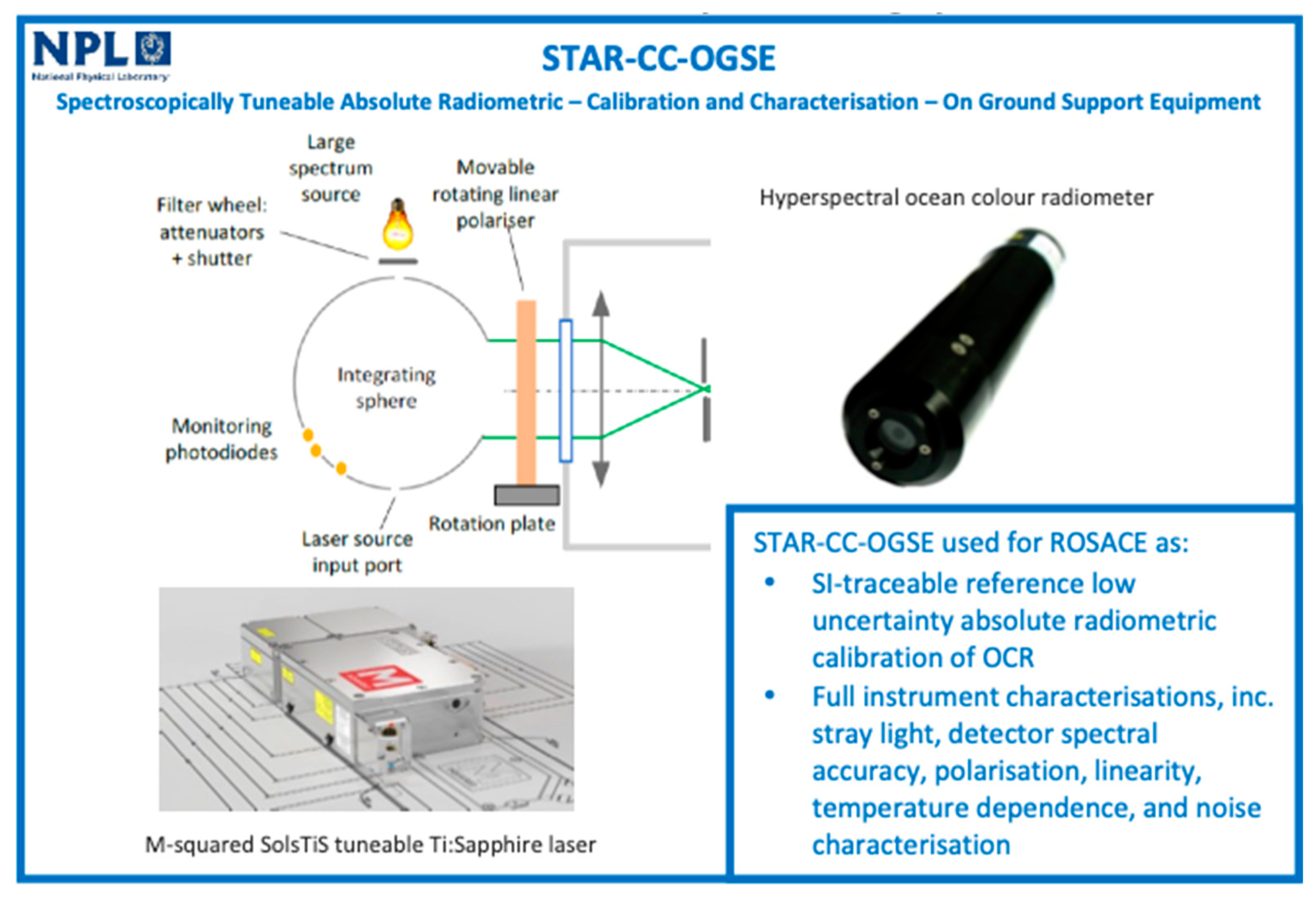
4.4.2. NMI Primary Absolute Radiometric Calibration and Characterisation: The STAR-CC-OGSE System

The STAR-CC-OGSE is a versatile facility for the radiometric calibration and characterisation of various sensors. This system is comprised of an integrating sphere fed by a tuneable Ti-Sapphire based laser (including harmonic generation) to produce a monochromatic radiance source. It allows monochromatic continuous tunability from 260 to 2700 nm (although more commonly available in more limited spectral ranges to suit customer applications). In addition, the same sphere includes a set of calibrated and uncalibrated lamps to produce a broadband (white light) radiation source extending over the same spectral extent. The sphere output is monitored by a set of monitoring photodiodes. The radiance of this system at chosen wavelengths can be calibrated with an uncertainty of better than 0.5% via a silicon trap detector that is itself calibrated against the NPL cryogenic radiometer [88]. The laser radiation is despeckled, depolarised and intensity stabilised.

The STAR-CC-OGSE comprises of two illumination systems each able to deliver broadband and monochromatic radiation:

• A large aperture SI-traceable calibrated integrating sphere source primarily for radiometric calibration and characterisation.
• A collimated beam source, equipped with an interchangeable, position fine-tuneable feature mask for optical performance characterisation. The features of the mask can be readily customised to suit various applications.

The main radiometric specifications of the STAR-CC-OGSE are listed in

Table 5. Main radiometric specifications of the STAR-OGSE-CC.

Radiometric source aperture size	Max. 200 mm diameter
Monochromatic spectral range	260–2700 nm
Broadband spectral range	250–2700 nm (equivalent to 3000 K blackbody).
Monochromatic typical radiance (radiometric sphere)	Over full spectral range 0.05 W m−2 sr−1 (laser bandwidth)−1 to 5 W m−2 sr−1 (laser bandwidth)−1 Corresponds to input laser power of 10 mW to 1 W
Broadband typical radiance	Variable in steps (ten times 10%) spectrally invariant. Max. > 3000 W m−2 sr−1 μm−1
Radiometric accuracy	<0.5% (in air/vacuum)
Radiance spatial uniformity	Typically <0.15% PV (application dependent)
Radiance temporal stability	<0.1% duration of a measurement
Monochromatic source line width	<0.2 pm
Monochromatic source tuning step size	<1–5 pm
Monochromatic source wavelength calibration	<0.2 pm (PV)
Calibrated TVAC-compatible radiance monitor	<0.5% (k = 1) [TBC]
Collimator focal length and F/#	1000 mm and F/5 (max collimated beam size 200 mm diameter)

.

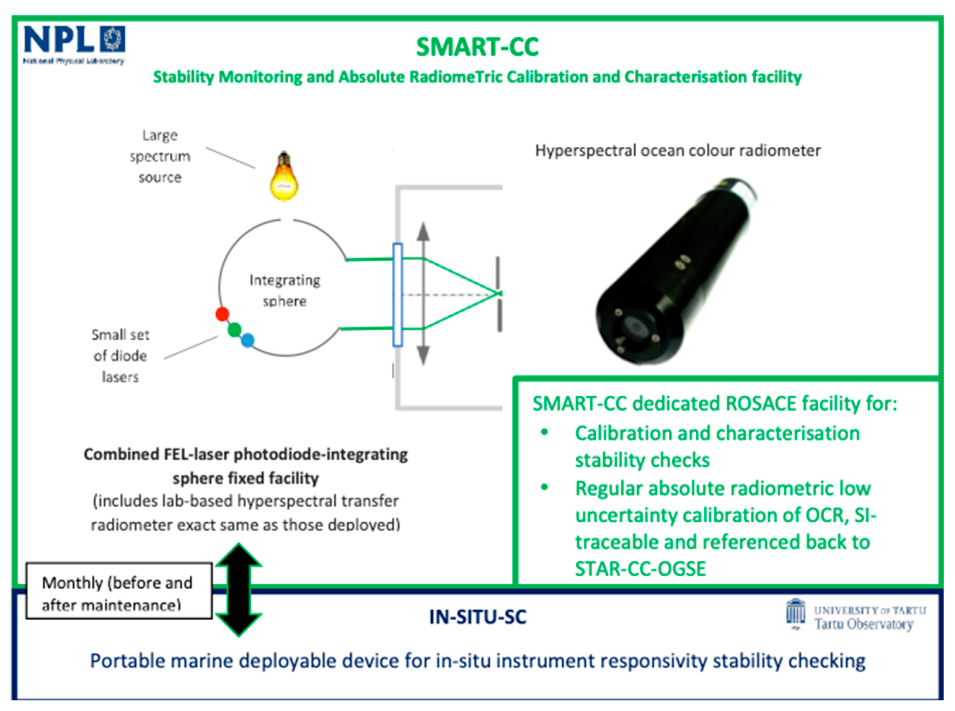
4.4.3. Site-Based Routine Absolute Radiometric Calibration: The SMART-CC System

This system will be developed by NPL and be permanently placed at LOV-IMEV and HCMR’s ROSACE calibration laboratories to allow for routine calibration and stability checks without the need for the instruments to be shipped. Using an integrating sphere-based system will reduce time and repeatability issues related to the traditional FEL and panel calibrations by minimising alignment efforts. The SMART-CC (Figure 23) will be an integrating sphere-based system allowing for absolute radiometric calibration, instrument stability checks and stray light and spectral calibration checks using a few key wavelengths. It can be seen as a mini version of the STAR-CC-OGSE without the tuneable laser option. This system will be calibrated at NPL on the SRIPS facility and will provide a broadband calibration source. It will have an accompanying calibrated radiometer to check for stability variance. In addition, diode lasers will be fed into the sphere providing a monochromatic source for selected wavelengths. Thus, this system will allow detection of any changes in spectral accuracy or stray light for the selected wavelengths. Any inconsistency detected using the SMART-CC system will have to be fully investigated by the STAR-CC-OGSE.

Some practical aspects of using the SMART-CC system are:

• Radiometer mounting: custom designed self-centring mounts to ensure the same position to within a few microns between calibrations.
• Light sources: the broadband source will be a quartz-tungsten-halogen (QTH) lamp. This may simply be a QTH bulb positioned at one of the sphere ports and powered with a suitable, stable power supply. For the greatest stability it is best to use a lamp in a housing with a feedback loop provided by an internal, thermoelectrically cooled photodiode. In addition, to minimize the use of the sphere surface for coupling, quasi-monochromatic sources such as temperature controlled single mode lasers, will feed into the sphere via optical fibre.
• Room stray light: to ensure external stray light does not affect the calibration of the radiometers, the SMART-CC system will be enclosed to block the ambient light during measurements.
• Sphere monitoring: silica detectors are well known to be linear over several decades’ incident optical power and stable over long periods of time. Use of a trap detector in the accompanying radiometer will allow identifying any drift in the SMART-CC system in excess of 0.2%.

4.4.4. Routine Relative Calibration in the Field: IN-SITU-SC

In order to follow possible changes in calibration and also biofouling contamination, a portable, field-deployable, relative calibration source will be developed for ROSACE. It will be used during buoy servicing to characterize the responsivity of complete instruments (including entrance optics) before and after cleaning. While the relative calibration source does not have to be SI-traceable, it must be well characterized and have good short-term stability (i.e., the duration of the cleaning and source measurements). Long-term stability of the source, i.e., stability across successive 6-month deployments of the radiometers, is not strictly required, but desirable and will be monitored with the SMART-CC.

A broadband emission in the VisNIR spectral range is needed and should not change with time or temperature. The radiant flux level and/or spectral shape will be easily switchable between pre-sets for validation of different instrument modes (e.g., upwelling radiance, downward irradiance). The instrument will be operable down to 20 m, be easily mounted onto underwater radiometers, and have an operating ambient temperature range of 10–30°. It will be battery powered and have slightly positive buoyancy so it is not lost in case of accidental release.

The solution proposed is based on LEDs, whose optical power and thermal control are needed to ensure constant intensity and spectral shape of the emitted light. The optical design concept suggested is presented in Figure 24a. The radiant flux from a white LED source is directed towards a diffusing window. The radiometer being tested measures the flux that is transmitted through the diffuser and is scattered forward towards the fore optics of the radiometer. An optical feedback photodiode (PD) measures the radiant flux that is backscattered from the diffuser. The photocurrent generated by the PD is used for adjusting the LED current.

The optical power and thermal control of the light source, the user interface for switching modes, and battery management will be handled by a main control unit (MCU). The MCU will also take care of monitoring and logging of internal environmental parameters (temperature and humidity) as well as light source operating parameters (current, voltage and LED temperature). All the logs will be time stamped using an internal real time clock and stored in a non-volatile memory for retrieval via the external interface after the field deployment. The subsystem module diagram of the IN-SITU-SC is shown in Figure 24b.

The mechanical design must be robust enough to tolerate field operations and moderate overpressure, yet light enough to be able to float on water and not sink if accidentally released by the diver. In addition, the mechanical design must be corrosion-resistant in a marine environment and provide sufficiently good heat transfer between the thermoelectric cooler of the LED and the surrounding water. The mechanical design should ensure a precise and repeatable mechanical fit to the spectrometer fore optics while blocking all possible ambient radiation. The surroundings of the optical output window must allow air bubbles to escape easily and prevent them getting trapped between the IN-SITU-SC and the entrance of the radiometer being validated.

4.4.5. Summary of the Calibration Strategy

In summary, the main elements of the calibration strategy for ROSACE are:

• STAR-CC-OGSE, allowing very low uncertainty absolute radiometric calibration and full radiometric characterisation using the new NPL tuneable laser system, to be used on brand new radiometers and then as needed (for example if a radiometer had to be repaired).
• SMART-CC: low uncertainty (1%–1.5%) regular calibration stability checks and absolute radiometric recalibrations of radiance sensors via instrument swap-out using the NPL designed non-tuneable laser-integrating sphere-FEL based system. If the results of these regular calibration and stability tests are unsatisfactory, for example showing significant change in radiometer responsivity, then the instruments are sent to NPL for recalibration/recharacterisation using the STAR-CC-OGSE.
• FEL lamps: regular calibration stability checks and absolute radiometric calibration of irradiance sensor using standard 1000 W quartz tungsten halogen lamps. These standards are regularly recalibrated at NPL after maximum 50 h of use.
• IN-SITU-SC: a field deployable relative calibration source to check stability of the optical instrumentation in situ during monthly maintenance cruises.
• In-air reality checks: a custom intercalibration bench will be developed to allow relative comparison between radiometers before and after deployment in realistic conditions. This will be realized by acquiring data with radiometers pointing toward the sun or a common target (calibrated blue fabric) in a natural environment (in air) not perturbed by reflections and shadowing and with a spectrum closer to what the instruments experience when deployed. These verifications extend the strict laboratory conditions in which the calibration is realized in order to detect possible anomalies in the radiometer response.

4.5. Biofouling Mitigation

At least three types of biological perturbations have to be taken into account when making radiometry measurements from an ocean buoy: biofouling on instrument collectors and housings, large biological organism shading/reflections, and biological waste.

Biofouling is unavoidable at sea and can have a strong impact on optical measurements. Several mitigation devices have been used in the past and have proven to be instrumental in increasing the number of bio-optical observations not affected by growing bacteria and larger marine organisms, for example the use of copper sheets, plates or robotic shutters and pulses of ultraviolet radiation. A combination of the copper and UV approach will be used for ROSACE [89,90].

Birds occasionally rest on buoys, which can generate shadow or deposit biological waste. The possibility to adapt existing auditory or mechanical devices to the marine environment for keeping birds away from the mooring will be considered [91]. Comparing the relative temporal changes in the above-water E_s and in-water E_d is also an efficient way to detect such anomalies, when both diverge in their changes (implemented for the BOUSSOLE data processing).

Moorings also unavoidably attract marine life. While very large marine organisms like cetaceans only occasionally swim close to moorings, smaller size fishes habitually find shelter and food close to moorings and can potentially perturb radiometric measurement. They can generate “peak” shadows or reflections, which are easily removed by filtering the raw data (because data are recorded at a high frequency during the acquisition sequences that last at least one minute). The presence of those fishes does not modify the bulk optical properties of the water mass, however.

5. Uncertainty Budget

5.1. Methodology

The guide to the expression of uncertainty in measurement (GUM) [92] provides a framework for how to determine and express the uncertainty of the measured value of a given measurand (the quantity that is being measured). Within the GUM framework, uncertainty analysis begins with understanding the measurement function and is then performed by considering in turn each of the different input quantities to the measurement function. Each input quantity may be influenced by one or more error effects, which are described by an uncertainty distribution. These separate distributions may then be combined to determine the uncertainty of the measurand, using the analytical method called the law of propagation of uncertainties or the numerical method using a Monte Carlo method (MCM) simulation that is summarized in the GUM supplement [93]. An example of BOUSSOLE’s in situ radiometric measurement uncertainty budget using MCM is described in [93].

In addition, we proposed to use a recently developed framework within the fidelity and uncertainty in climate data records from Earth observations (FIDUCEO) [94] project. This framework applies rigorous GUM-based metrological methods to satellite sensor fundamental climate data records (FCDRs) [95], where a schematic representation of the measurement function, called the uncertainty tree diagram, formed the basis of the analysis (Figure 25).

At the centre of this diagram is the measurement function—here with the measurand as water-leaving radiance, $L_w$, and input quantities such as underwater upwelling radiance at depth z₁, $L_{u,z_1}$, and the attenuation coefficient for the nadir upward radiance, $K_u$. From this function, branches spread out from each input quantity, which may themselves be determined by their own measurement functions (for example here $K_u$ is determined from the upwelling radiance measurements acquired at two different depths), to their uncertainty. This uncertainty can be traced back through to its impact on the measurand by the sensitivity coefficients on each branch. Finally, the effects that cause each respective uncertainty are connected to the end of each branch.

Note that we should also consider the extent to which the measurement function describes the true physical state of the instrument, which is accounted for by including the term +0 at the end of the measurement function. This explicitly represents effects that are expected to have a zero mean and are not captured by the measurement function (i.e., there is an uncertainty associated with this quantity being zero).

Each of the effects identified at the end of each of the branches should then be understood, quantified and reported in an “Effects Table” that documents:

• The uncertainty associated with the given effect.
• The sensitivity coefficient required to propagate the uncertainties associated with that effect to uncertainty associated with the measurand.
• The correlation structure over spatial, temporal and spectral dimensions for errors from this effect.

Table 6. Table for codifying the uncertainty due to an error effect and its correlation structure.

Table Descriptor		How This is Codified
Name of effect		A unique name for each source of uncertainty in a term of the measurement function
Affected term in measurement function		Name and standard symbol of affected term
Instruments in the series affected		Identifier of the specific instrument/deployment where this effect matters
Correlation type and form	Temporal within deployment	Forms of correlation described in detail in [96]
	Temporal between deployments
	Spectral (hyperspectral in-situ)
Correlation scale	Temporal within deployment	In units of spectral pixels, measurements or deployments in time—what is the scale of the correlation shape?
	Temporal between deployments
	Spectral (hyperspectral in-situ)
Channel/band	List of channels affected	OLCI channel names in standard form
	Error correlation coefficient matrix	OLCI cross-channel correlation matrix
Uncertainty	PDF shape	Functional form of estimated error distribution for the term
	units	Units in which PDF shape is expressed
	magnitude	Value(s) or parameterisation estimating the PDF width
Sensitivity coefficient		Value, equation or parameterisation of sensitivity of measurand to term

shows an adapted form of the FIDUCEO “Effects Table” for use in describing error effects in the OC-SVC process, with description of how it should be populated.

A full description of all components presented in Figure 25 and examples of their effects tables are provided in Appendix A.

To propagate uncertainty for the measurands of interest (water-leaving radiance, downward irradiance, water-leaving reflectance and normalised water-leaving reflectance) we proposed the following approach.

Measurement functions are defined based on the tree diagrams, including all raw inputs (see Figure 25), and which are defined as quantities that can have an influence on the measurand values. These were used for all processing steps rather than intermediate quantities (for example $K_u$ in the calculation of $L_w$). All raw inputs have their standard uncertainty identified in terms of magnitude (value) and probability distribution function (PDF). Due to the complexity of the measurement function it is challenging to derive all sensitivity coefficients analytically (for example $\frac{\partial L_w}{\partial Chl}$ or $\frac{\partial L_w}{\partial z_{sensor}}$ would be extremely difficult), thus we proposed using MCM to propagate the raw inputs uncertainties using a measurement function. We handled the partial correlation between some input quantities (for example, the absolute radiometric calibration coefficients of the different instruments) by decomposing these to a set of variables that are independent of each other (though these independent variables may themselves be correlated through time).

The final uncertainty value will be derived from the PDF of the output values generated through the MCM. All uncertainties will be reported with the k = 1 coverage factor. The uncertainties will be evaluated for water-leaving radiance, downward irradiance and water-leaving reflectance as an output of the field segment, and normalised water-leaving reflectance as the input to the gains calculation. They will be reported as one value for each of these outputs, and then split into three categories of random, fully correlated within one deployment and fully correlated within a satellite mission’s lifetime.

The evaluation of the uncertainties of individual matchup and mission average OC-SVC gains will not be under the responsibility of the OC-SVC infrastructure. However, we recommended estimating the uncertainties of the mission averaged OC-SVC gains including different temporal correlation terms:

$$u^2\left(\overline{g}\right)=\frac{{{\displaystyle \sum }}_i{u}_{\mathrm{rand}}^2\left(g_i\right)}{N}+\frac{{{\displaystyle \sum }}_j{\left[\frac{1}{N_j}{{\displaystyle \sum }}_k{u}_{\mathrm{d}\mathrm{sys}}\left(g_k\right)\right]}^2}{M}+{\left[\frac{1}{N}{\displaystyle \sum }_i{u}_{\mathrm{sys}}\left(g_i\right)\right]}^2$$

(4)

where $\overline{g}$ is the mission average gain, $g_i$ is individual matchup gains, $N$ is the total number of matchups and $M$ is a number of deployments that have correlated inputs. $N_j$ is the number of matchups in a given deployment, $j$, where $g_k$ are the subset of individual matchups in that deployment.

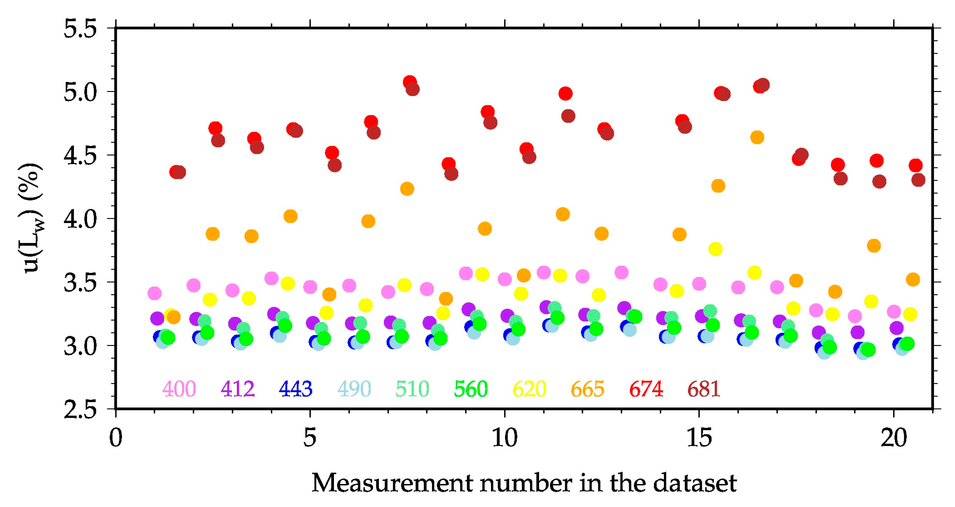
5.2. Preliminary Uncertainty Budget

A demonstration data set was created from BOUSSOLE in situ hyperspectral data, by selecting data that are considered a priori suitable for the OC-SVC process based on environmental parameters such as the buoy tilt or the SZA. This data set covers the period from May 2016 to March 2017, during which 20 valid matchups were found for the S3A/OLCI overpasses.

The uncertainties were evaluated using the measurement equation presented in Figure 25 and the method described in [94]. The existing absolute calibration capabilities were used to estimate radiometric calibration uncertainties. In addition, instrument characteristics such as stray light and detector linearity were incorporated into the model and corrected for using the methods presented in [96]. Relative uncertainty for water-leaving radiance is shown in Figure 26 for twenty in situ measurements and the first ten S3A/OLCI spectral bands. The results indicate uncertainties generally below 3.5% for the spectral bands 1-7 covering the spectral range from 400 to 620 nm, then increasing to about 5% for longer wavelengths.

Table 7. Relative uncertainties (%, k = 1) in water-leaving radiance for the matchup number 15.

OLCI Band (nm) and band (no.)	400 (1)	412.5 (2)	442.5 (3)	490 (4)	510 (5)	560 (6)	620 (7)	665 (8)	673.75 (9)	681.25 (10)
Current BOUSSOLE radiometers	3.5	3.2	3.1	3.1	3.3	3.2	3.8	4.3	4.9	4.9
Anticipated new ROSACE radiometers	2.8	2.4	2.3	2.3	2.6	2.5	3.1	3.8	4.6	4.6

presents the results of the same simulation run for the hypothetical new optical system with a new calibration facility for measurement number 15. The environmental conditions for this measurement seem to be close to perfect as the measured buoy tilt was −1.3° and 1.2° for x and y axes, respectively, and [TChl-a] was 0.11 mg m⁻³.

A significant reduction in uncertainty values could be anticipated for the shorter wavelengths where the instrument-related effects, which were small, had a larger relative impact on the overall uncertainty values. The reduction was smaller for the longer wavelengths for which the environmental conditions and modelling applied in the processing chain were the main relative contributors to the uncertainty values.

The proposed methodology addresses in detail the uncertainty propagation process, considering the temporal scale correlations present in mission averaged gain calculation. The practical realization of this method can be incorporated in the data processing chain and would enable evaluation of an uncertainty per measurement, always including appropriate ancillary data. This method therefore provides a concept of dynamic uncertainty per in situ measurement and matchup that we considered the most appropriate for both MSEA and BOUSSOLE as Copernicus OC-SVC.

6. The Ground Segment

6.1. Role and General Architecture

The ROSACE ground segment sits at the interface between the OC-SVC field component (field sites) and the ground segment of the satellite mission. It takes raw data from the field sites and performs all processing and quality control (QC) operations needed to generate the fully qualified data that the OC-SVC process requires. This section described the preliminary design of this ground segment, which will be located in, and operated from, ACRI-ST premises in Sophia Antipolis, France (Figure 27). The ground segment included near-real time, adjusted and delayed modes of data processing (NRT, AM and DM, respectively).

• The NRT processing was performed as soon as the data were received from the buoys, with products generated on the fly along with their quality flag and uncertainty estimates, following automatic and documented procedures (including QC. See Section 6.4 and Section 6.5). An additional functionality will allow the site operator to change the QC flags through a semisupervised quality control interface. This information, i.e., the change of flag and its old and new value, will be incorporated into the NRT product.
• The adjusted mode (AM) products were generated by using data collected during monthly servicing cruises, when the instrumentation onboard the ROSACE buoys were cleaned, checked and maintained. During these operations, in situ sampling and radiometric profiles will be carried out. These data will be used for adjusting the instrument calibration for data collected during the previous month, and therefore to readjust the processing. Existing data products were thus reprocessed with these updated inputs.
• The delayed mode (DM) products will be generated through reanalysis of a longer time series of data, typically every 6 months at each rotation of instrumentation. This processing step allows better assessment of the overall consistency of the data (e.g., by examining seasonality, trends and comparison with climatology). The results of this reanalysis might lead to changes in the products’ annotations.

Each of the data product types will by default contain the value of the parameter and its time of acquisition, its uncertainty and QC flags.

6.2. Data Products and Levels

Raw data (RD) from the radiometric, optical and physical payloads were received in near-real time (NRT) from the buoys. They were converted into geophysical units with instrument-specific calibration coefficients, which are part of the auxiliary data (AD). These RD could be processed to derive statistically representative values at a lower frequency than the initial data, referred to as basic products (BP). For instance, a single representative value of L_u(z) at a given depth was derived from the (60 × v) individual measurements available from a 1-min acquisition sequence of an instrument collecting data at frequency v (Hz).

As for the radiometry measurements, these BP will include the upwelling nadir radiance and the downward irradiance at the measurement depths, L_u(z) and E_d(z), and the above-water downward irradiance (E_s) at the native spectral resolution of the ROSACE radiometers. BP will also include diagnostic and ancillary data useful to monitor the status of the deployment platform and instruments in NRT.

Primary and secondary products (PP and SP, respectively) were then derived from the BP in conjunction with the data from instrument characterisation, modelling or other external sources (also included in the definition of AD). The SP was the same radiometric quantities corrected for instrument and environmental errors, data used for QC or by-products used to generate the PP. These included for example the diffuse attenuation coefficients for radiance and downward irradiance (K_L and K_d respectively, (m⁻¹)).

The PP were the highest-level products, to be directly ingested into the SVC process generated both at full spectral resolution and for the spectral bands of any satellite instrument under consideration, through convolution with the spectral bands response functions of that sensor (here the OLCI instruments aboard the S3 satellite series):

• The spectral fully-normalised water-leaving radiance, [L_w]_N (W m⁻² nm⁻¹ sr⁻¹).
• The remote-sensing reflectance, R_rs (sr⁻¹).

The equations involved in the derivation of PP and SP are available in [16,28] and were not detailed here.

These radiometric data products were stored along with other data in a single database that eventually included:

• Optical data products, including the normalized water leaving radiance used for OC-SVC.
• Platform data products, e.g., buoy tilt.
• Metocean data products, e.g., wave conditions and wind speed.
• Calibration and correction data, e.g., calibration gains.
• Configuration management parameters, e.g., processor version.
• Logbooks including operators’ comments on specific situations and the local environmental background.

Data will be safeguarded using an archival system that includes a daily automatic backup of the in situ datasets. A 50 TB shared disk space is available at ACRI-ST, which is secured due to a Quantum iScalar 80 library of LTO5 drives. This system will be used to backup the entire ROSACE data and software, avoiding data losses.

6.3. Data Processing and Storage

The data processing in the ROSACE ground segment is illustrated in Figure 27 (note that for readability, archiving and storage are not shown). It will be a centralised entity, linked to local transmission centres that are dedicated to each of the OC-SVC field segments. In addition, it is intended to be almost fully automatic and triggered by data availability, with no human interaction other than the following exceptions:

• The configuration (e.g., of calibration or correction, depending on [TChl-a], etc.) may evolve from one rotation of the optical system or buoy to the other and then the corresponding parts of the database will need to be updated (manually) by maintaining the versioning in the database.
• The QC macro flags can be updated by an operator through a semisupervised quality control (SSQC— see Section 6.4.
• The data need to be reprocessed (back in time) each time there is an update in the configuration files.

6.4. Semisupervised Quality Control

As soon as the raw data are processed and available to the database, the operator can visualize them through a dashboard. The main capabilities of this tool are, in short:

• To check the product at each stage of its elaboration (from raw data to the final product).
• To check its consistency with respect to previous acquisitions and/or ancillary information from on-site campaigns or Metocean or satellite data.
• To visualize all related contextual information (e.g., sea state, platform behaviour) and auxiliary products that have been used to derive the consolidated product, its uncertainty and its quality annotation.

The dashboard will also allow the operator to:

• Annotate the product with a specific text comment that will be stored in the equivalent of a logbook.
• Raise a new quality flag on the product. This new flag will be added in parallel to the flag that was given automatically by the processing system (i.e., the initial flag is not replaced). This allows traceability of flagging.

Note that by ‘operator’ we mean a user who is an expert on the particular site and has been given relevant access rights to the system and database. Access to this dashboard will be allowed to any user after registration but will be limited to data consultation (no annotation) and, after a period of time, dedicated to product consolidation.

A similar SSQC system is operated for the biogeochemical (BGC-) Argo floats through a system available on-line (www.seasiderendezvous.eu [97]). In summary the ROSACE SSQC will have a similar functionality that will include:

• A hierarchical visualization web tool allowing any operator to navigate from a higher level product down to initial raw data while at the same time having access to all associated uncertainties and contextual information.
• The capability to annotate the data by adding a new QC flag value, and/or providing a comment in a textual form that will be stored in a log book.
• The capability to edit and consult the logbook.
• The capability to communicate with other operators, at other sites, through a simple chat system. This capability is also extended to communication between operators and the ROSACE ground segment manager.
• The capability to extract information in a simple file format (e.g., csv) to allow extra analysis.

6.5. Final QC

This final stage (stage 8—see Figure 27) represents a key component in the data product elaboration and evaluation. It consists of assigning confidence metrics and uncertainty to the final product that is delivered to the OC-SVC processing system.

Qualitative assessment:

All elementary flags that were evaluated at each stage of the process (stages 1 to 7—see Figure 27) will be combined to derive a global QC flag for each of the final products. These flags will follow the standard that has been adopted in the in situ thematic assembly centre (INSTAC) of the Copernicus marine service (i.e., (0) no QC applied, (1) good data, (2) probably good data, (3) bad data potentially correctable, (4) bad data and (5) value changed). The algorithm and rules that will be used to combine the elementary flags will be defined during the specification and design phase. Qualitative assessment is seen as a confidence rating attached to ROSACE products ensuring that all elements entering into the product derivation have been in line with acceptable ranges and expectations.

Quantitative assessment:

A model has been developed to provide estimates of the uncertainty (as an absolute value or percentage) of the final product used in the OC-SVC process [94]. This uncertainty model will be refined to be in line with the final data processing (Section 5.1). The final purpose is to quantitatively assess the data products and deliver three levels of data quality (Q1, Q2 and Q3) depending on their relative uncertainty, and to do this for each processing mode (NRT, AM and DM). In addition, a flag will identify products suitable for matchup analyses based on a combination of criteria (e.g., cloud filtering etc.).

Table 8. Examples of data quality levels as a function of the data uncertainty.

PHASE	Q1	Q2	Q3
NRT	u% < 3	3 ≤ u% ≤ 5	u% > 5
DM	u% < 3	3 ≤ u% ≤ 5	u% > 5
AM	u% < 3	3 ≤ u% ≤ 5	u% > 5

shows an example of how the different phases and quality levels might combine according to relative uncertainty levels (u%). Different u% could be attributed to different wavelengths.

Both quantitative and qualitative evaluations will be attached to the final products delivered to the OC-SVC centre, allowing an informed selection of which set of measurements are eventually used for the gain computations.

7. Infrastructure Operations

7.1. Field Segment

The two field sites, BOUSSOLE and MSEA, will be coordinated by LOV-IMEV and HCMR, respectively. As such, they will be responsible for the calibration, deployment, monitoring, maintenance and recovery of the optical system radiometers (OSR) at the two sites. Each site will have three OSR sets available to rotate in the field. This will be with the support of NPL for the characterization of the OSR and recalibration of standards, of CIMEL for OSR and acquisition/transmission unit refurbishment and UT-TO and NPL for yearly round robin intercalibrations. LOV-IMEV and HCMR, with the support of ACRI-IN, will also be responsible for the deployment, monitoring, maintenance, recovery and refurbishment of the full mooring line, buoy upper superstructure and buoy lower superstructure, as well as the installation of the OSR on the platform.

LOV-IMEV and HCMR will conduct monthly cruises at the buoy site for maintenance, deployment of the IN-SITU-SC and of ship-deployed optical systems (free-fall profiling radiometers). They will ensure transfer of information to the ground segment for all aspects that might have an impact on data quality. They will transmit auxiliary and cruise data to the ground segment. LOV-IMEV and HCMR will also organize on demand cruises for extraordinary maintenance of the buoys’ optical system and platform. LOV-IMEV and HCMR will also ensure transfer of information to the ground segment for all aspects that might have an impact on data quality and will transmit auxiliary and cruise data to the ground segment.

These activities at both sites will be supported by human and material resources committed by the national institutes as a significant in-kind support. For instance, these contributions have represented half of the total budget needed to run BOUSSOLE on average over 2003–2019. Funding of the other half was equally shared between ESA and the French space agency (CNES). A similar model is proposed for ROSACE.

Absolute calibration of the three OSR at each site will be performed before and after their deployment at sea with a 6-month rotation that is independent from the platform deployment (i.e., divers can swap out instruments in the field). Pre- and post-calibrations will be complemented by reality checks of the instrumentation, which consist of “in air” relative intercalibrations of OSR against the sky or a diffuser target. These verification and calibration processes will be the basis to decide whether or not the instrument needs on demand module replacements/repairs at CIMEL and recharacterisation at NPL.

Visual inspection of the OSR in the field will also be performed on a monthly basis by divers and technical staff. Refurbishment of the OSR will be performed at CIMEL after every three rotations in the field. The profiling system radiometers (PSR) will be calibrated at the same time as the OSR. A systematic refurbishment of the PSR every 2 years will also be performed at CIMEL. In-air intercalibration of the PSR will be integrated with the OSR in-air intercalibration.

An intercalibration round robin will be performed every year with a profiling transfer radiometer. This will consist of absolute calibration at LOV-IMEV, HCMR and UT-TO, and field deployment at BOUSSOLE and MSEA along with the PSR in the vicinity of the buoys. CIMEL and UT-TO will also act as a technology work group to maintain the state of the art of the optical system, whereas NPL will have the same role for absolute calibration standards and protocols. LOV-IMEV and HCMR will act as the technology work group for field segment operational activities in connection with the supervisor of platform maintenance.

7.2. Ground Segment

The operational ROSACE ground segment (GS) will be run by ACRI-ST. This GS will operate in both a NRT and an off-line mode. The NRT mode will process the field segment data as soon as they are available, and the off-line mode will reprocess the data back in time from the starting date when a new configuration has been applied.

Preventive maintenance, i.e., adaptation to information technology and operating system evolutions, will take place at a frequency of 6 months to one year during operations. Adaptive maintenance will also occur during the operations, and includes implementation of new or improved algorithms and QC procedures.

LOV-IMEV and HCMR will contribute to development of the data processing and quality control procedures in connection with the ground segment team.

7.3. Governance

A consortium of European Institutions and SMEs proposes the ROSACE infrastructure. With such an involvement of several entities, an appropriate governance structure has to be put in place, so that coordination of all activities is ensured, the overall schedule of the project is maintained, and possible evolutions of the infrastructure are adequately phased in.

A project office will oversee the activity, working closely with the five teams dedicated to the main technical functions of the infrastructure. These five teams will manage the optical system and calibration, the deployment platform, the field segment, the ground segment, and the SI-traceability, metrology aspects and uncertainty budget. The project office will be the main interface with EUMETSAT on scientific, administrative and financial matters. It will evaluate and validate the project deliverables and reports, coordinate the project on a day-to-day basis, monitor the overall progress and milestones, organise reviews and meetings, manage all administrative and financial matters.

A steering committee will be responsible for the strategic management and decision making in the project, which will include recommending possible directions/choices for the ROSACE project, evaluating the results achieved and making recommendations about strategic directions, performing risk assessment and suggesting strategies if issues arise, ensuring links with the scientific community and international groups (e.g., IOCCG) and anticipating evolutions in OC-SVC.

A technical advisory board composed of a team of international independent experts will support the development of the infrastructure, by providing recommendations, expertise and by reviewing the activity in an on-going manner.

The project office and steering committee will also promote the scientific exploitation of data collected by the ROSACE OC-SVC infrastructure via dedicated research projects, with attention to improvements in optical measurement protocols, uncertainty estimates, correction methodologies, QC procedures and the OC-SVC process.

Possible innovations will be discussed within the steering committee under EUMETSAT and Copernicus oversight. They will be tested for a sufficiently long time in parallel to operational standards in order to ensure continuity and a robust evaluation before integration into the operational activities.

8. The Profiling Float Network Option

8.1. Increasing the Matchup Capacity of the Infrastructure

Collecting radiometry measurements from autonomous profiling floats is gaining increasing attention in the oceanographic and Earth observation communities. Such floats, whose initial use was for measuring temperature and salinity over the global oceans (Argo programme [98]), now come with various payload configurations including an increasing number of instruments [99]. Some of these floats include radiometers, and their data have been used for satellite OCR validation purposes [100,101]. An advanced float including a specifically designed radiometer system has recently been proposed as an option that meets most of the requirements for the OC-SVC of the future NASA PACE mission [102].

Our approach here was not to use profiling floats as a central element of the OC-SVC infrastructure, but as an option to improve the matchup capacity of the infrastructure and eventually extend its footprint beyond the fixed sites. This extension allows confirmation of the OC-SVC gains and uncertainties, and will allow increasing the matchup capability during the commissioning phase of future elements of the Sentinel-3 constellation (e.g., S3C and S3D). About 50 matchups are needed to get stable OC-SVC gains [3]. A network of floats working in conjunction with the fixed sites could help reach this number faster. For this combination to be effective, the radiometry from the floats should, however, be fully consistent with the radiometry from the fixed sites. This is among the specifications that have been set for the development of the new ROSACE radiometer.

8.2. The ProVal Float and its ROSACE Upgrade

The development of a float dedicated to satellite OCR validation started in 2011 at LOV-IMEV. The float is named ProVal [25] and uses a two-arm configuration inspired by the BOUSSOLE mooring. It allows for two identical radiometers to be hosted on either side of the float. Both sensors measure the downward irradiance (E_d) and the upwelling nadir radiance (L_u). With this configuration the irradiance sensors are at 21 cm depth and the radiance sensors at 45 cm depth when the float is at surface, which is referred to as the “buoy mode”. Platform shading issues are mitigated by always having one sensor outside of the float’s shadow. This configuration also ensures data redundancy, which is helpful to monitor the relative behaviour of the instruments over time and for QC.

Vertical E_d and L_u profiles are acquired during the ascending phase with increasing depth resolution from parking depth to surface (e.g., every 1 m up to 60 m and every 10 cm up to the surface). When the float reaches the surface, one minute of data acquisition occurs in “buoy mode”. Four instances of the remote sensing reflectance (R_rs) are generated from the collected data. Two are obtained by extrapolating to the surface the vertical E_d and L_u profiles of both pairs of radiometers, and two are generated from the data collected by both pairs of radiometers during the “buoy mode”. The profiling sequence can be modified remotely, following trade-offs between the amount of data to be transmitted, the available energy and the data transmission costs. Rescheduling the float mission is also feasible remotely, including maintaining the float at surface for recovery.

The profiling mode described above would generate about 140 KB per profile, which would take 12 min to be sent back to the ground segment via satellite transmission. A single float will have enough energy to perform 300 such profiles.

First deployments of ProVal floats exhibited very good navigation behaviour in terms of tilt, vertical ascent speed and capacity to target a particular surfacing time. They also show a very good matchup probability with S3/OLCI of about 20% (

Table 9. Matchups ratio for three deployments in the Mediterranean Sea with S3 OLCI.

Mission ID	Deployment Start Date	Area	Number of Profiles	Matchups Ratio
Lovapm006f	09/06/2017	BOUSSOLE	81	29%
Lovapm006h	11/06/2018	Ionian Sea	101	18%
Lovapm006i	26/09/2019	MSEA	35	23%

), which expresses how many profiles are needed to generate a matchup. Note that the difference in matchups ratio between BOUSSOLE and MSEA may be related to the season. A July deployment at MSEA would likely end up with a higher matchup ratio. The matchup processing is described in [25] and mainly follows validation criteria.

Modifications of the current ProVal platform will be necessary to meet the ROSACE requirements. These include:

• Implementation of the new fit-for-purpose CIMEL radiometer, which will require, in particular, an increased depth rating as compared to the version to be installed on the buoys.
• Development of on-board data processing in order to make NRT transmission possible despite the large amount of data generated by hyperspectral radiometers. A new acquisition board is under development for the next generation of ProVal floats, which will be used for the ROSACE floats. The full data set can be downloaded at float recovery.
• Inclusion of a rechargeable battery. Opening a float to swap batteries is time consuming and may compromise waterproofness of the float, so we will implement a rechargeable battery as is done now on gliders [103].

8.3. Minimum Configuration and Operations

One float will be available at each site to increase the sampling and matchup capability during operation of the Sentinel constellation, in particular during the satellite’s critical phases, e.g., commissioning phase or programmed band shifts. These floats may also be used as a backup in case the main mooring is unavailable.

The human resources required to operate a float depends essentially on how often it is repositioned on site. At the BOUSSOLE site, a repositioning every two weeks will probably be sufficient but this frequency may have to be higher for MSEA because of the proximity of small islands. This will be adjusted according to the season and prevailing circulation patterns. During each recovery, the float will be cleaned and the sensors compared with the portable, field-deployable, relative calibration source. Every 150 profiles, the float will be brought back to the laboratory to recharge the batteries and recalibrate the sensors. Nonetheless the centralized ground segment and the simplicity of deployment/recovery of such a platform, make it flexible enough to envision different scenarios of operations to fit the evolving requirements of OC-SVC and Copernicus marine services.

9. Conclusions

A European solution was proposed for an infrastructure serving the OC-SVC needs of the Copernicus Sentinel-3 operational missions. It is named ROSACE, which stands for radiometry for ocean colour satellites calibration and community engagement, and has been described in this paper. Key features that can be highlighted in these concluding remarks are that ROSACE:

• Answers all OC-SVC requirements that were established in [21].
• Includes two sites (BOUSSOLE and MSEA) that are demonstrably suited to providing a large number of OC-SVC-quality matchups every year.
• Minimises risks because it builds on an existing quasi-operational capability (BOUSSOLE).
• Minimises the development time, because of the above point, plus it exploits existing expertise and elements that can still be used in the meantime before a new system becomes fully operational.
• Minimises costs for delivering the requirement of multiple sites.
• Maintains, optimises and expands current European expertise in order to provide a coordinated effort and sovereignty for the Copernicus OCR SVC infrastructure.

High-level rationales and features were presented in this paper, while details of existing elements forming the base of the proposed infrastructure were not repeated when already available in the literature, e.g., the full description of the BOUSSOLE buoy design and testing [80,81,82], the associated overall project structure and realisations [16,28], the details of published surveys indicating MSEA as the best location for OC-SVC in European waters [20,22,23,24], the data processing protocols [28], the approach to delivering per-measurement uncertainties [94] or the characteristics and preliminary achievements of the ProVal floats [25]. Further details about the proposed new elements, e.g., the fit-for-purpose hyperspectral radiometers or the MSEA site, will become available and published in the open literature when mature enough.

The emphasis was put here on the main items that demonstrate compliance of the proposed infrastructure with OC-SVC requirements described in [29]. This report includes 62 requirements, the compliance of ROSACE with all relevant ones (numbers 9–62) having been demonstrated in [29]. The corresponding compliance matrix was not replicated here. This full compliance was reached by combining outstanding expertise and knowledge in OC-SVC gained over the past 20 years at BOUSSOLE with a number of new developments. The growth from a long-term project run by essentially a single research group (BOUSSOLE) to an integrated and operational European infrastructure (ROSACE) is feasible through bringing together European expertise of partners who already have a history of collaboration, and through including new elements and technology.

As a matter of conclusion, we show the combined OC-SVC matchup capability of BOUSSOLE and MOBY (Figure 28), which is likely the best way of demonstrating the above claims about what ROSACE could deliver with BOUSSOLE and MSEA working together. The capability illustrated in Figure 28 for BOUSSOLE is already significant and indeed is used in support of the Copernicus Sentinels [104], although it is actually below the minimum capability of the proposed ROSACE infrastructure, which has the potential of delivering up to about 80 high-quality matchups every year from the combination of BOUSSOLE and MSEA.