Article

Detection of Collapsed Buildings in Post-Earthquake Remote Sensing Images Based on the Improved YOLOv3

1
Aerospace Information Research Institute, Chinese Academy of Sciences, Beijing 100101, China
2
University of Chinese Academy of Sciences, Beijing 100101, China
*
Author to whom correspondence should be addressed.
Remote Sens. 2020, 12(1), 44; https://doi.org/10.3390/rs12010044
Submission received: 4 November 2019 / Revised: 12 December 2019 / Accepted: 16 December 2019 / Published: 20 December 2019

Abstract

:
An important and effective method for the preliminary mitigation and relief of an earthquake is the rapid estimation of building damage via high spatial resolution remote sensing technology. Traditional object detection methods only use artificially designed shallow features on post-earthquake remote sensing images, which are uncertain and complex background environment and time-consuming feature selection. The satisfactory results from them are often difficult. Therefore, this study aims to apply the object detection method You Only Look Once (YOLOv3) based on the convolutional neural network (CNN) to locate collapsed buildings from post-earthquake remote sensing images. Moreover, YOLOv3 was improved to obtain more effective detection results. First, we replaced the Darknet53 CNN in YOLOv3 with the lightweight CNN ShuffleNet v2. Second, the prediction box center point, XY loss, and prediction box width and height, WH loss, in the loss function was replaced with the generalized intersection over union (GIoU) loss. Experiments performed using the improved YOLOv3 model, with high spatial resolution aerial remote sensing images at resolutions of 0.5 m after the Yushu and Wenchuan earthquakes, show a significant reduction in the number of parameters, detection speed of up to 29.23 f/s, and target precision of 90.89%. Compared with the general YOLOv3, the detection speed improved by 5.21 f/s and its precision improved by 5.24%. Moreover, the improved model had stronger noise immunity capabilities, which indicates a significant improvement in the model’s generalization. Therefore, this improved YOLOv3 model is effective for the detection of collapsed buildings in post-earthquake high-resolution remote sensing images.

Graphical Abstract

1. Introduction

Acquiring information on building damage immediately after an earthquake is key to rescue and reconstruction efforts [1]. Although the accuracy and degree of confidence of the acquitted data via traditional manual field survey methods are relatively high, there are certain shortcomings, such as large workload, low efficiency, the high cost associated with acquisition, and data unfit for presentations, that render these methods unable to conform to the requirements for rapid acquisition of the information of interest [2]. With progress in sensor and space technologies, remote sensing techniques can acquire detailed spatial and temporal information of the target area, which is widely used to monitor natural disasters [3,4]. Previous studies have proven that remote sensing data can extract relatively accurate information on building damage [5].
For the extraction of information on building damage from remote sensing images, previous studies have investigated numerous methods, which can currently be divided into multi- and single-temporal evaluation methods. The multi-temporal evaluation method is mainly based on detecting changes to evaluate the information on building damage. Gong et al. [6] used high-resolution remote sensing images from before and after the 2010 Yushu earthquake as examples for the extraction of information on building damage based on the object-oriented change detection, pixel-based change detection, and principal component analysis-based change detection methods. The results showed that the object-oriented change detection method had the highest accuracy for extracting information on building damage. However, due to effects from data acquisition, such as revisit cycles, shooting angle, time, and other factors, the application of the multi-temporal evaluation method is difficult in practice [7]. For the single-temporal evaluation method, data acquired via remote sensing after an earthquake has less constraints, such that it has become an effective technical means that can be directly used to extract and evaluate information on building damage [8]. Janalipour et al. [9] used high spatial resolution remote sensing images as background to manually select and extract features based on the fuzzy genetic algorithm, establishing a semi-automatic detection system for building damage. This system has increased robustness and precision compared with machine learning methods, such as the random forest (RF) and support vector machine (SVM). However, the single-temporal evaluation method is also characterized by certain problems, such as difficulties associated with feature space selection. Moreover, due to certain factors, such as background noise and illumination changes in remote sensing images, classifier performance is seriously affected [10], resulting in problems with obtaining accurate extractions of information on building damage via traditional detection methods.
In recent years, object detection methods based on deep learning have made significant breakthroughs for natural images, which can be divided into region- and regression-based methods. Since the breakthrough of the region-based convolutional neural network (R-CNN) [11] for natural images, the combination of a region-based extractor and detection network has become a classic paradigm. In region-based object detection methods, the proposed object box can be generated and then transmitted to the deep convolutional neural network (CNN) for classification and location regression in the second stage. Although the accuracy of methods, such as Faster R-CNN [12] and Mask R-CNN [13] are relatively high, they are unable to conform to the requirements of real-time applications. Apart from region-based object detection methods, we have regression-based methods, including You Only Look Once (YOLO) [14], Single Shot Multi-Box Detector (SSD) [15], YOLOv2 [16], and YOLOv3 [17], among others. These methods use a single CNN to simultaneously predict the boundary box and classify, and transform the object detection problem into a regression problem. Therefore, the regression-based object detection method can significantly shorten the time required for detection, which is feasible in practical applications. As the capability of generalization of features extracted by the CNN is much higher than traditional artificial features, the CNN can be rapidly applied to object detection of remote sensing images. Han et al. [18] proposed an improved Faster R-CNN algorithm, which performed an integration process by sharing the characteristics of the region proposal and object detection phases. This improved the Faster R-CNN method, which has a higher accuracy than other CNN-based models for datasets with a spatial resolution of 10 meters (NWPU (Northwestern Polytechnical University) VHR (very-high-resolution)-10 [19]) labeled by Northwestern Polytechnical University. Zheng et al. [20] improved the structure of YOLOv3 and tested aircraft high- and low-quality (due to overexposure and cloud occlusion) remote sensing images. The results showed that the improved framework yielded 99.72% and 98.34% for the accuracy and recall rate respectively, which was better than the original YOLOv3 model. Especially for the low-quality remote sensing images, there was a significant improvement in the accuracy. However, the current object detection method based on the CNN has rarely been applied to the extraction of information on damaged buildings affected by earthquakes, and mainly stays at the classification of damaged buildings with CNN. Duarte et al. [21] combined satellite images with manned and unmanned aerial vehicle (UAV) aerial images to construct samples of damaged buildings, which improved the quality and quantity of the samples, and adopted the CNN framework based on the residual connection and expansion convolution to improve the classification effect. Ji et al. [22] used the CNN and building vector boundary to classify buildings from post-earthquake satellite images and identify collapsed buildings. They proposed solutions to the sample imbalance problem between collapsed and non-collapsed buildings. However, this method requires a building vector map, which has certain restrictions for applications.
These studies have shown that the YOLO series of algorithms have a better generalization capability and faster detection speed than the R-CNN series of algorithms. Therefore, to achieve higher efficiency and precision when detecting single-collapsed buildings in post-earthquake remote sensing images, we use the YOLOv3, a CNN-based object detection method. The main aim of this study is to use the YOLOv3 model to efficiently and accurately detect collapsed buildings in post-earthquake remote sensing images. We not only investigate ways to use the model to detect collapsed buildings, but also improve a part of its network structure and loss function to improve the efficiency and accuracy of detection.
The rest of this paper is organized as follows. Section 2 describes the study area and details of the model improvements. Section 3 describes the results evaluation indicators and experimental settings. Section 4 presents the analysis of the experimental results. Section 5 discusses the improved model. Finally, Section 6 concludes this paper.

2. Materials and Methods

2.1. Dataset

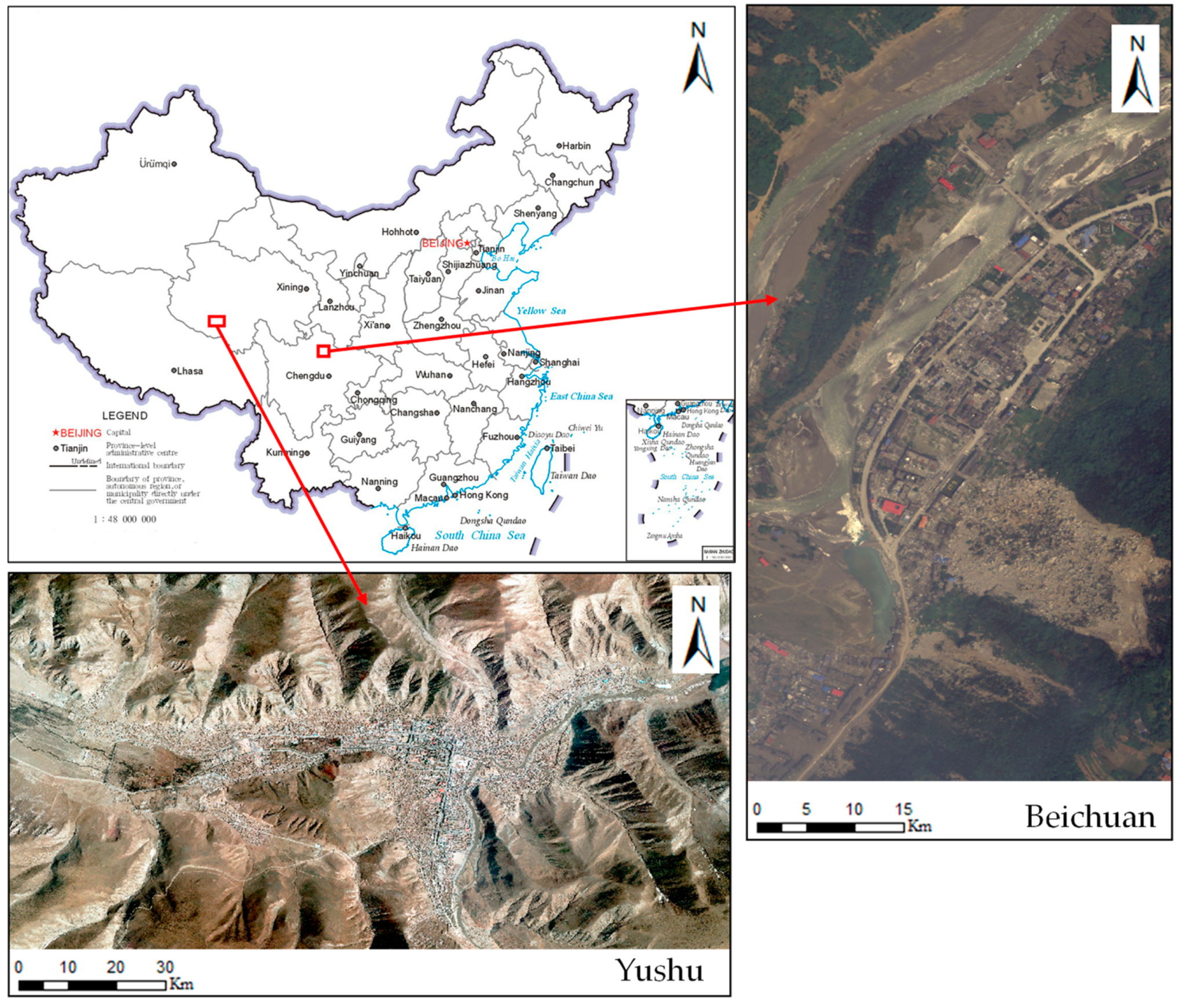
2.1.1. Remote Sensing Data Acquisition

Materials to test the effectiveness of the proposed method, we selected aerial remote sensing images acquired on the second day after the 7.1 magnitude earthquake that occurred in the Yushu Tibetan Autonomous Prefecture of the Qinghai Province on 14 April 2010 and aerial remote sensing images from Beichuan County after the Wenchuan earthquake that occurred on 12 May 2008. These images included a large number of collapsed and non-collapsed buildings with a data resolution of 0.5 m. The location of the study area is shown in Figure 1.

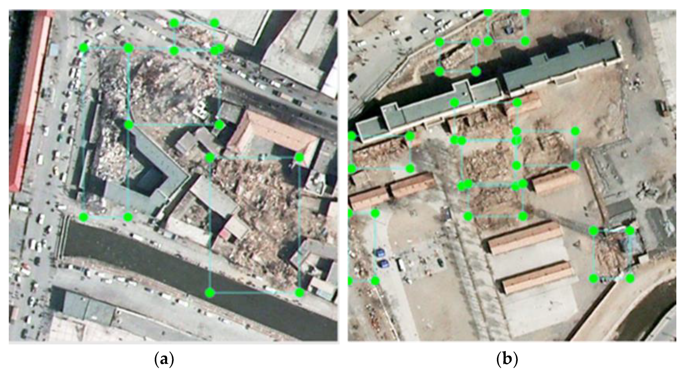
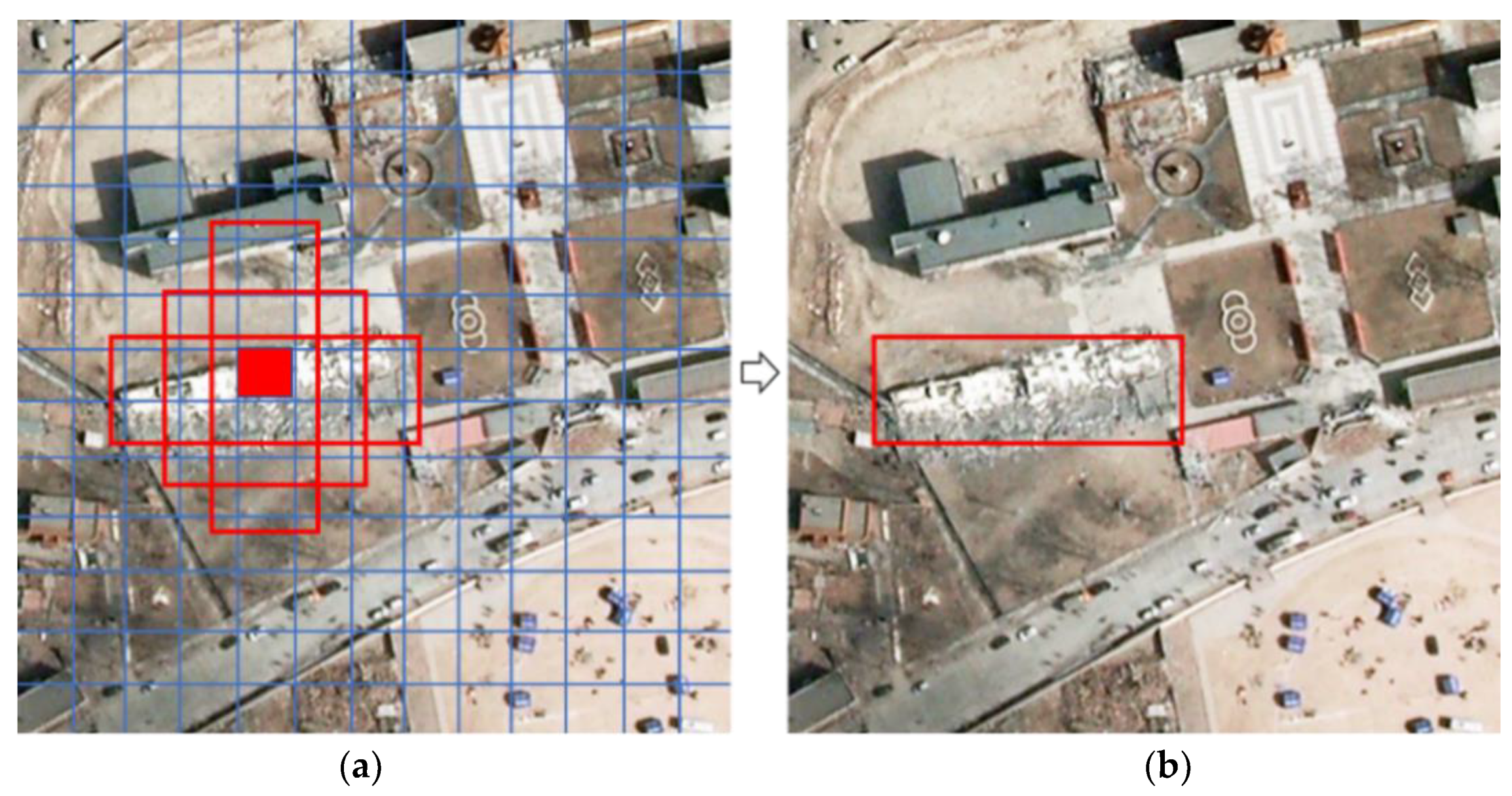
2.1.2. Dataset Production

The acquired remote sensing images cannot be directly input into the deep learning model. They need to be cut to obtain image blocks of the size specified in the YOLOv3 model. Therefore, image blocks each of 416 pixels × 416 pixels were first cut out of the large remote sensing images, each containing a certain number of collapsed and non-collapsed buildings. Subsequently, the LabelImg software was used to label collapsed buildings in the image block in PASCAL VOC [23] format, as shown in Figure 2.

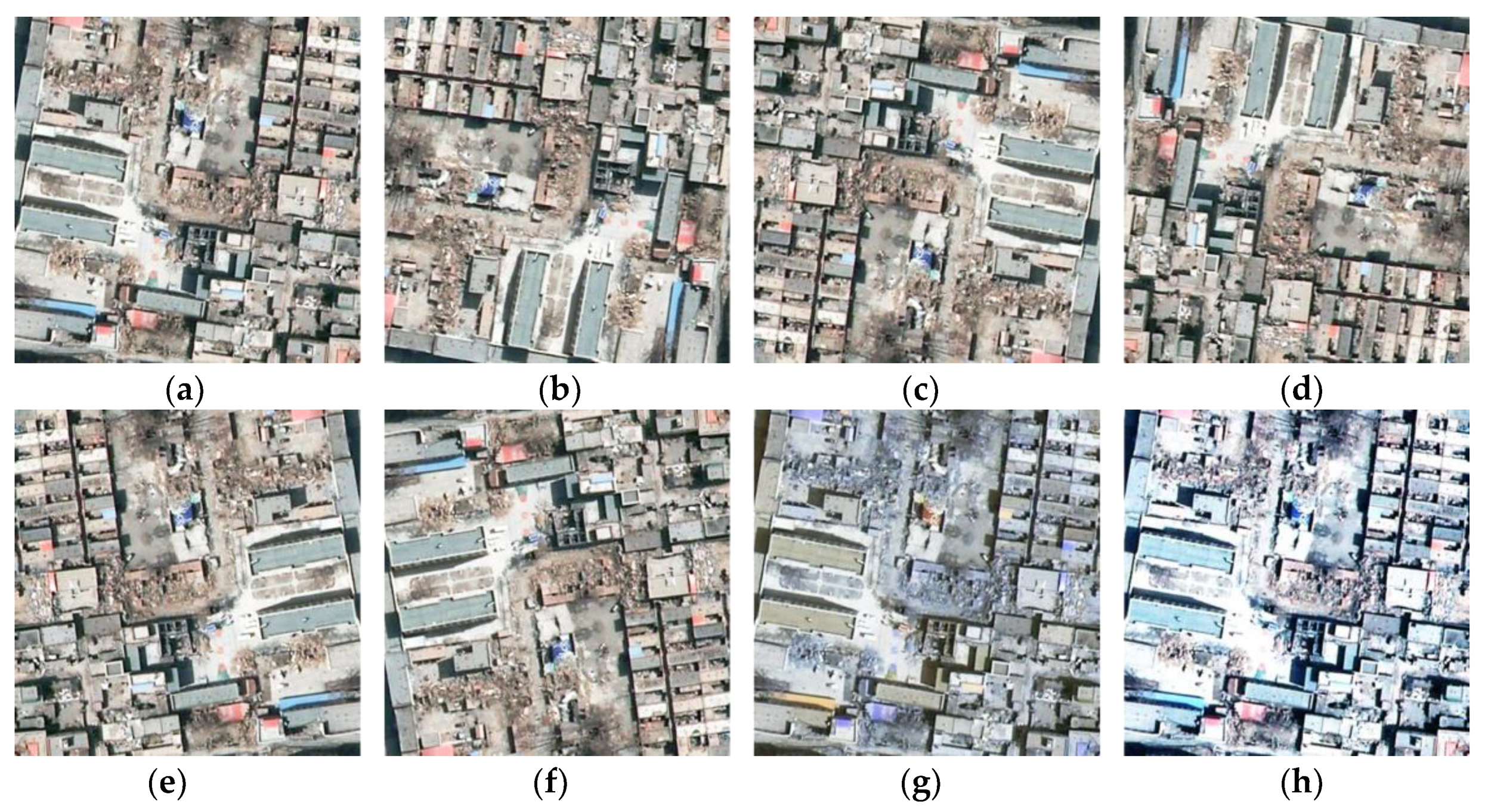
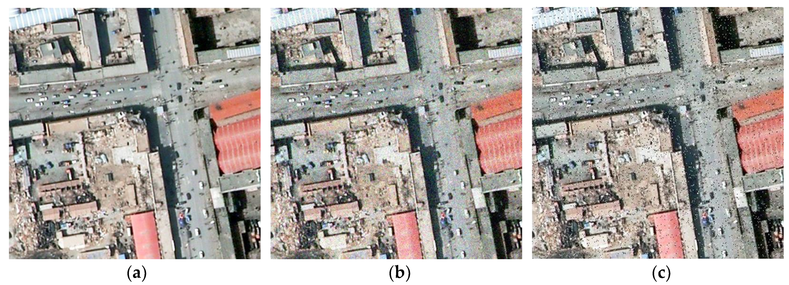
2.1.3. Dataset Enhancement
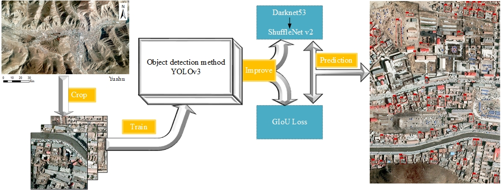
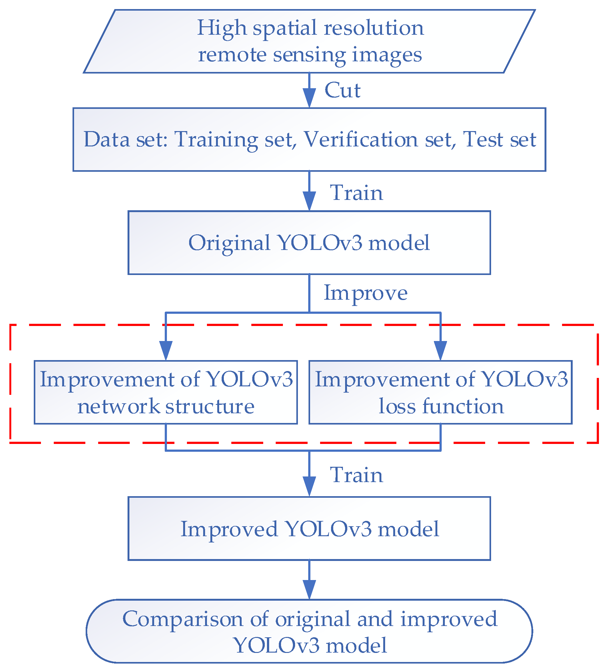
Data enhancement for deep learning datasets is usually performed in a way similar to natural images, and involves rotation, flipping, increasing noise, and color transformation, among other [24]. For image rotation and flipping, the main operations are the rotations by 90, 180, and 270 degrees, horizontal, and up-and-down flipping. The rotated and flipped images can improve the detection performance of the model. For image color transformation, because the color of the image obtained under different sensors and environments will be biased, color transformation is needed to eliminate the influence of color deviation on model performance. However, there are some differences between the enhancement methods for remote sensing images and those for natural images. For example, most objects in natural images typically only rotate at small angles, whereas, in this study, the buildings can be rotated at any angle. In addition, remote sensing images are often displayed after stretching, such that the data after stretching and enhancements can yield a more robust model.
After screening, the final selected enhancement methods were image rotation, image flip, color transformation, and image stretching, as shown in Figure 3. Through enhancement, a total of 2180 sample images were obtained, which were then divided into three groups, namely the training set for training the model, the verification set for verifying the model during training, and the test set for evaluating the model. Many collapsed buildings are included in the sample images, the specific number of which is shown in Table 1.

2.2. Method Flow

The main aim of this study was to use the YOLOv3 model to efficiently and accurately detect collapsed buildings in post-earthquake remote sensing images. However, to detect only collapsed buildings, the parameters of the feature extraction layer in the YOLOv3 network are too complex and redundant, which may lead to over-fitting, i.e., the training accuracy is high, while the test accuracy is low. Therefore, the network structure of YOLOv3 model was improved to reduce the complexity of network structure. In addition, based on the improvement of YOLOv3 network structure, the loss function was also optimized. Finally, the method flow in this paper is shown in Figure 4. The red dotted line in the figure is the improvement and optimization of the network structure and loss function of the YOLOv3 model.

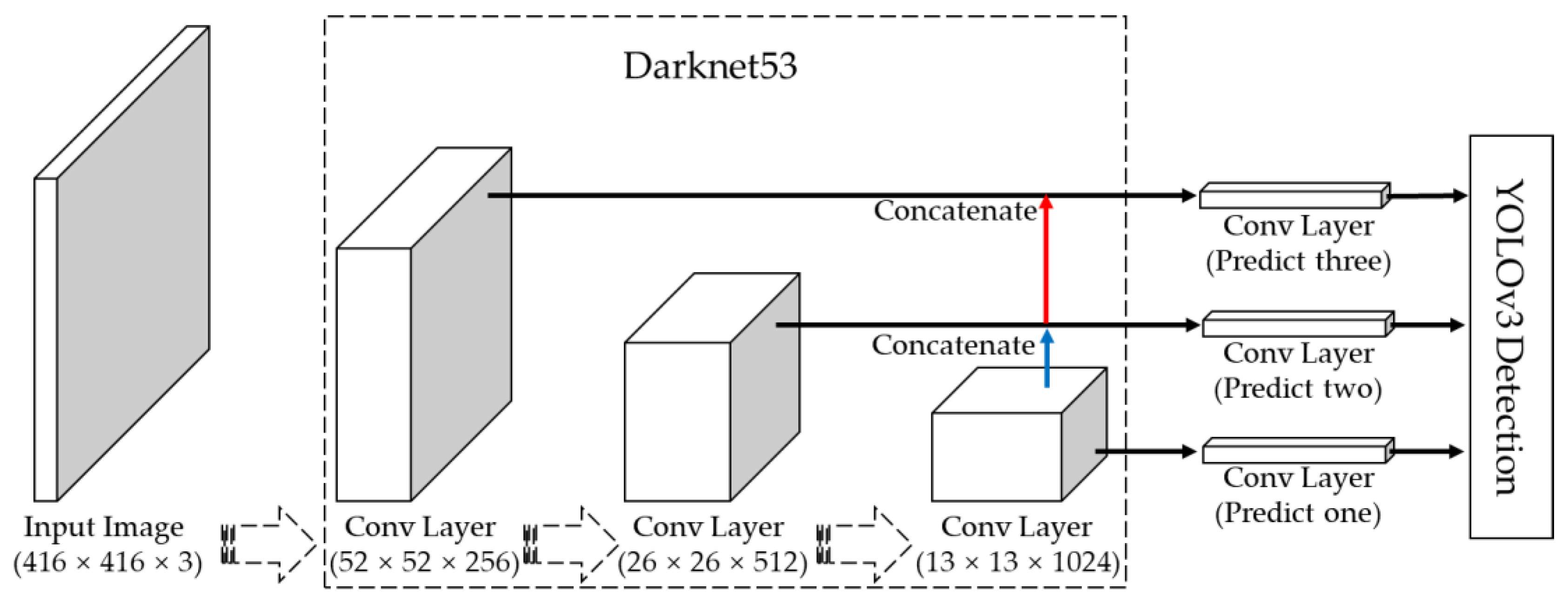
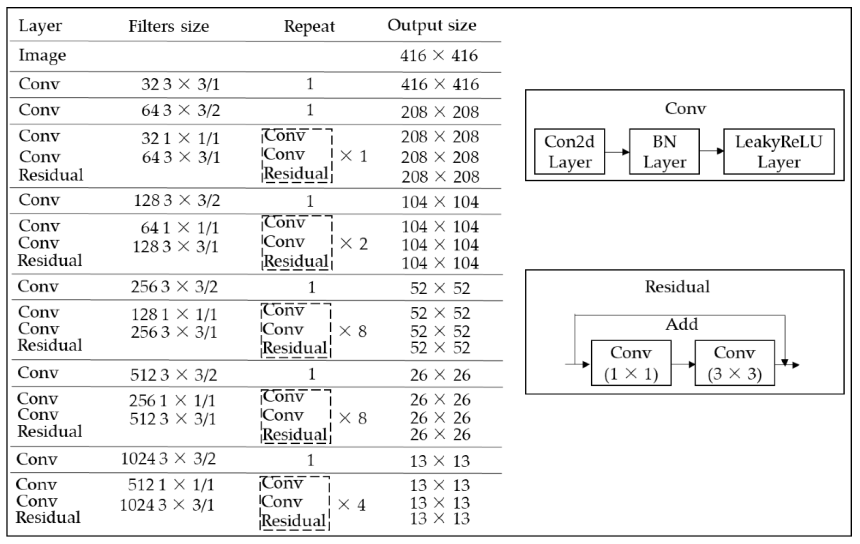
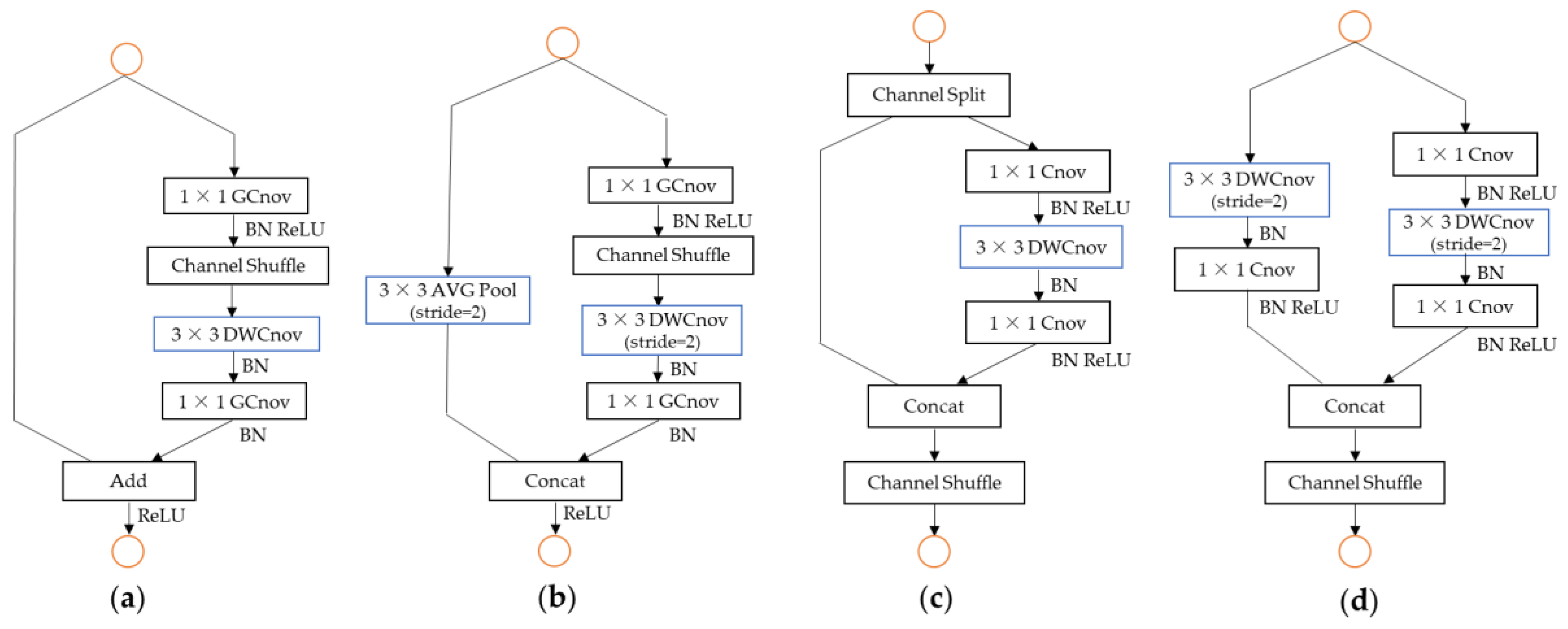
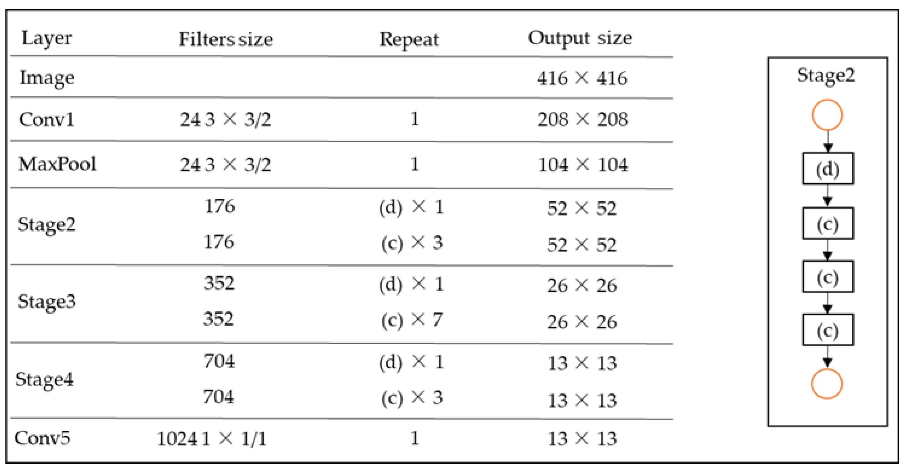
2.3. Improved YOLOv3 Network Structure

The YOLO series algorithms are originally target recognition methods based on regression proposed by Redmon et al. [14]. By 2018, YOLO had been developed into its third generation, i.e., YOLOv3, which has a rapid detection speed and high detection accuracy for small and dense targets. YOLOv3 uses the multi-scale prediction method to improve the defects of YOLOv2 for small target recognition, significantly improving the recognition accuracy of small targets while maintaining the rapid detection speed of YOLOv2. Therefore, YOLOv3 has a high detection accuracy and fast speed. Figure 5 shows the YOLOv3 network structure. First, YOLOv3 scale the original image to a size of 416 pixels × 416 pixels. After extraction of features with Darknet53, the original image is transformed into a feature map with a size of 13 × 13. Three feature maps are formed by combining two feature maps with sizes of 26 × 26 and 52 × 52. In other words, detection is performed on three scales, such that the feature map is transmitted to the two adjacent scales using twice the up-sampling. On each feature map, each cell predicts three bounding boxes by means of three anchor boxes, finally selecting the most suitable bounding box, which is shown in Figure 6. For each bounding box, the network predicts its center point (XY), width and height (WH), confidence, and category. For an input image, the final output dimension is 1 × ((13 × 13 + 26 × 26 + 52 × 52) × 3) × (5 + k) = 1 × 10,647 × (5 + k), where k represents the number of categories.
In YOLOv3, the Darknet53 convolution network is the feature extractor, which is shown in Figure 7. Darknet53 is mainly composed of a series of convolution layers at dimensions of 1 × 1 and 3 × 3, with a total of 53 layers (including the last fully connected layer but excluding the residual layer). Each convolution layer is followed by a batch normalization (BN) [25] layer and LeakyReLU layer. A number of residual network modules were introduced in Darknet53, i.e., the residual layer shown in Figure 7, which was derived from ResNet [26]. The purpose of adding the residual layer is to solve the gradient disappearance or gradient explosion problems in the network, such that we can more easily control the propagation of the gradient and perform network training.
In Darknet53, although numerous 1 × 1 convolution kernels were introduced and 3 × 3 convolution kernels, with a step size of 2, were used instead of the maximum pooling, the number of parameters was reduced a lot. However, to detect the single-class objects in this study, the Darknet53 network still appeared to be slightly complicated and redundant. To reduce the number of parameters in the YOLOv3 model and improve its detection speed, we replaced the Darknet53 feature extraction network with the lightweight ShuffleNet v2 [27] network in this study.
ShuffleNet v2 is a lightweight classification network proposed in 2018, which introduced the idea of depth-wise convolution [28] and group convolution. The shuffling and grouping operations in ShuffleNet v1 [29] are continually used, which allowed ShuffleNet v2 to perform at a higher precision while increasing the running speed. In ShuffleNet v2, Ma et al. [27] proposed the following four conclusions as criteria to improve the running speed:
  • Conclusion 1. When the feature channels of the convolution layer for the input and output are equal, the MAC (memory access cost) is the smallest, whereas the model speed is the fastest.
  • Conclusion 2. Excessive grouping convolution will increase the MAC and slow down the model’s running speed.
  • Conclusion 3. Fewer branches in the model results in a more rapid model running speed.
  • Conclusion 4. The time consumption of the element-wise operations is much higher than that of the floating-point operations. Therefore, it is necessary to reduce the element-wise operations as much as possible.
Based on these four conclusions, the basic unit of ShuffleNet v2 was proposed, which is shown in Figure 8c–d. Among the units, Figure 8a–b is the basic units of ShuffleNet v1. Based on a comparison of Figure 8a,c, it shows as follows: first, Figure 8c added a channel split operation at the beginning, which had the same number of input and output channels, corresponding to Conclusion 1. Second, in Figure 8c, the grouping operation in the 1 × 1 convolution layer was cancelled. At the same time, the channel split operation was added to the front to only divide the number of channels into two groups, corresponding to Conclusion 2. Third, the operation of the channel shuffle in Figure 8c moved to the end of the Concat operation, corresponding to Conclusion 3. Finally, the Concat operation was replaced with the element-wise operation, Add, corresponding to Conclusion 4. A comparison of Figure 8b,d was essentially the same. Figure 8b,d is mainly used to reduce the scale and increase the number of channels.
Figure 9 shows the network structure of ShuffleNet v2, where each stage consists of basic units (c) and (d) shown in Figure 8. The number of each basic unit corresponds to the Repeat column shown in Figure 9.

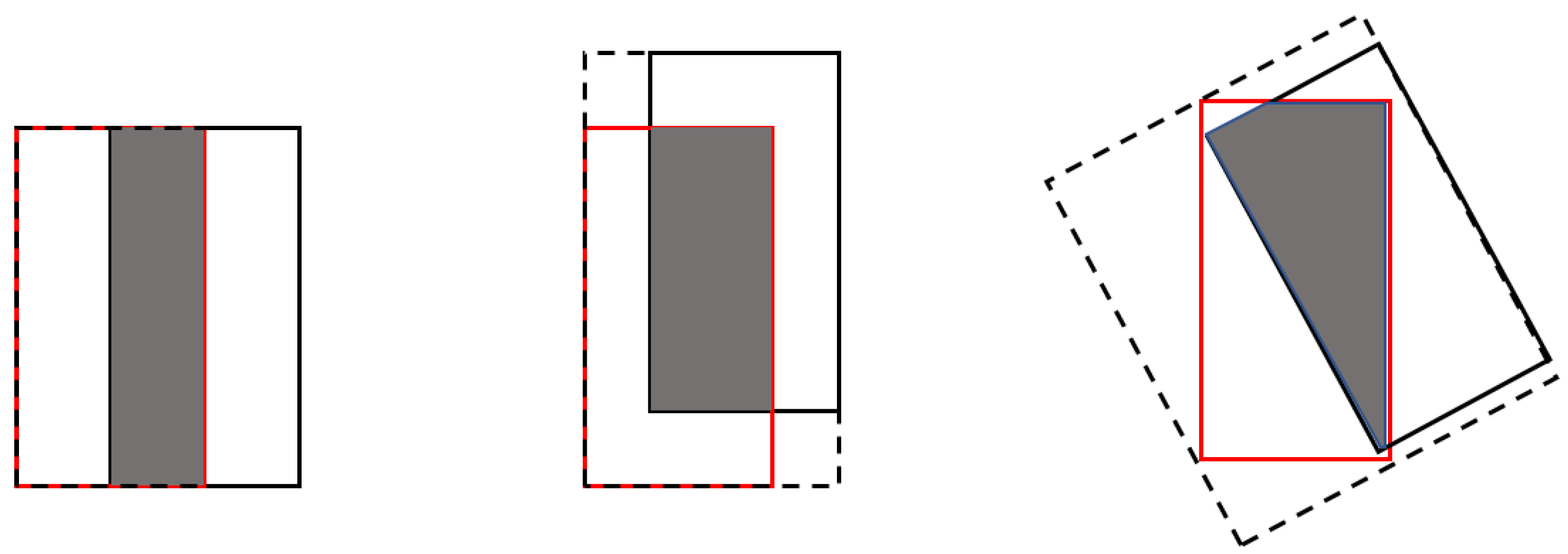
2.4. Improved YOLOv3 Loss Function

During the training process, the YOLOv3 loss function is divided into three major parts, i.e., coordinate loss, confidence loss and classification loss, which can be expressed with the following equation:
L o s s = i = 0 10647 ( C o o r d L o s s + C o f i d e n c e L o s s + C l a s s L o s s ) ,
where CoordLoss is the coordinate loss, ConfidenceLoss is the confidence loss, and ClassLoss is the classification loss. The coordinate loss is the XY loss plus WH loss in prediction box. In YOLOv1 version, X, Y, W, and H directly predict the actual value of the object, where small changes in the predicted value expand to the entire range of the image, resulting in large coordinate fluctuations and inaccurate predictions. YOLOv2 improved upon these problems, and can be expressed with the following equation:
X = σ ( t x ) + c x ,
Y = σ ( t y ) + c y ,
W = p w e t w ,
H = p h e t h ,
where t x and t y are the network prediction values, which are scaled to between 0 and 1 via the Sigmoid operation, c x and c y are the cell coordinates on the feature map, i.e., the offset from the upper left corner, t w and t h are also the network prediction value, and p w and p h represent the width and height, respectively, of the cell corresponding to the anchor box.
Based on Equations (2) and (3), we found that the center point coordinates X and Y of the prediction box are activated by the sigmoid function. Figure 10 shows the characteristics of the sigmoid function and its derivative curve. When the output of the neural network is large, the derivative of the sigmoid function becomes exceedingly small. At this time, the error value obtained using the squared error is exceedingly small, leading to a slow convergence speed for the network.
To solve the above problem when the real value can only be 0 or 1, the common method is to adopt the cross-entropy loss function, which can be expressed with the following equation:
L o s s = 1 n i = 1 n [ a i l o g ( a ^ i ) + ( 1 a i ) l o g ( 1 a ^ i ) ] ,
where a i is the true value and a ^ i is the output value after the Sigmoid function. When the true value, a i , can only take 0 or 1, the cross-entropy loss function meets the requirements. In other words, when a i and a ^ i are equal to 0, the error can be obtained from Equation (6), which is near 0. Similarly, when a i = 1 and a ^ i = 1 , the error is also near 0. For the prediction box center point coordinate, XY, however, the true value is neither 0 or 1 but, rather, a value between 0 and 1. For example, when a i = a ^ i = 0.6 , the cross entropy loss is 0.6 × log ( 0.6 ) 0.4 × log ( 0.4 ) = 0.29 , not 0. Therefore, the loss function for the center point coordinate, XY, can be improved.
To improve the loss function of the center coordinate, XY, we used the generalized intersection over union (GIoU) [30]. GIoU is an improved version of the traditional intersection over union (IoU), which can replace the regression parameters for the distance loss of the prediction box. There are two reasons as to why we have proposed the use of the GIoU as the regression loss function for the prediction box rather than an IoU for the loss function. The first is that, when IoU ( A , B ) = 0 , we cannot know if A and B are adjacent to each other or far apart. The other reason is that the IoU cannot reflect the overlap situation for the two rectangular boxes. For example, the three cases shown in Figure 11 have different overlapping situations, i.e., the GIoU values, from left to right, are 0.33, 0.24, and −0.1, whereas the IoU value is 0.33.
However, the IoU still has several advantages. For example, the IoU can be used as the distance and has scale invariance. Therefore, to resolve the disadvantages of the IoU and retain its advantages, we used the GIoU, which can be calculated as follows:
G I o U = I o U | C \ ( A B ) | | C | ,
where C is the minimum enclosing rectangle of A and B, and C \ ( A B ) is C minus ( A B ) . The GIoU has the following properties. First, it has the scale invariance property. Second, the GIoU is less than or equal to the IoU. Third, the GIoU can better reflect the overlap between the two rectangular boxes shown in Figure 11. Fourth, 1 GIoU 1 . When A = B , GIoU = IoU = 1 . When A does not intersect B and is far away, GIoU tends to be −1. Therefore, we selected 1 GIoU as the loss function, which ranged from 0 to 2.

3. Experimental Settings

3.1. Evaluation Indicators

To quantitatively evaluate the performance of the selected models, we adopted the average precision (AP) and precision recall curve (PRC). In addition, the F1 score [31] and FPS (frames per second) were used to evaluate the model’s performance and detection speed.

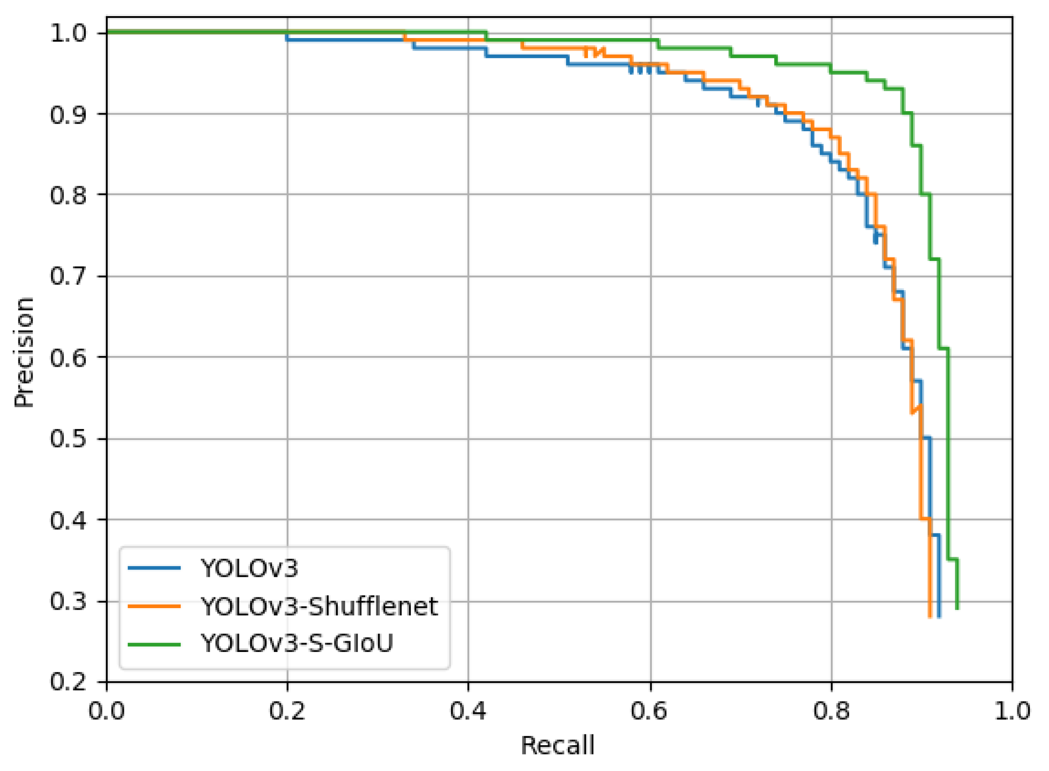
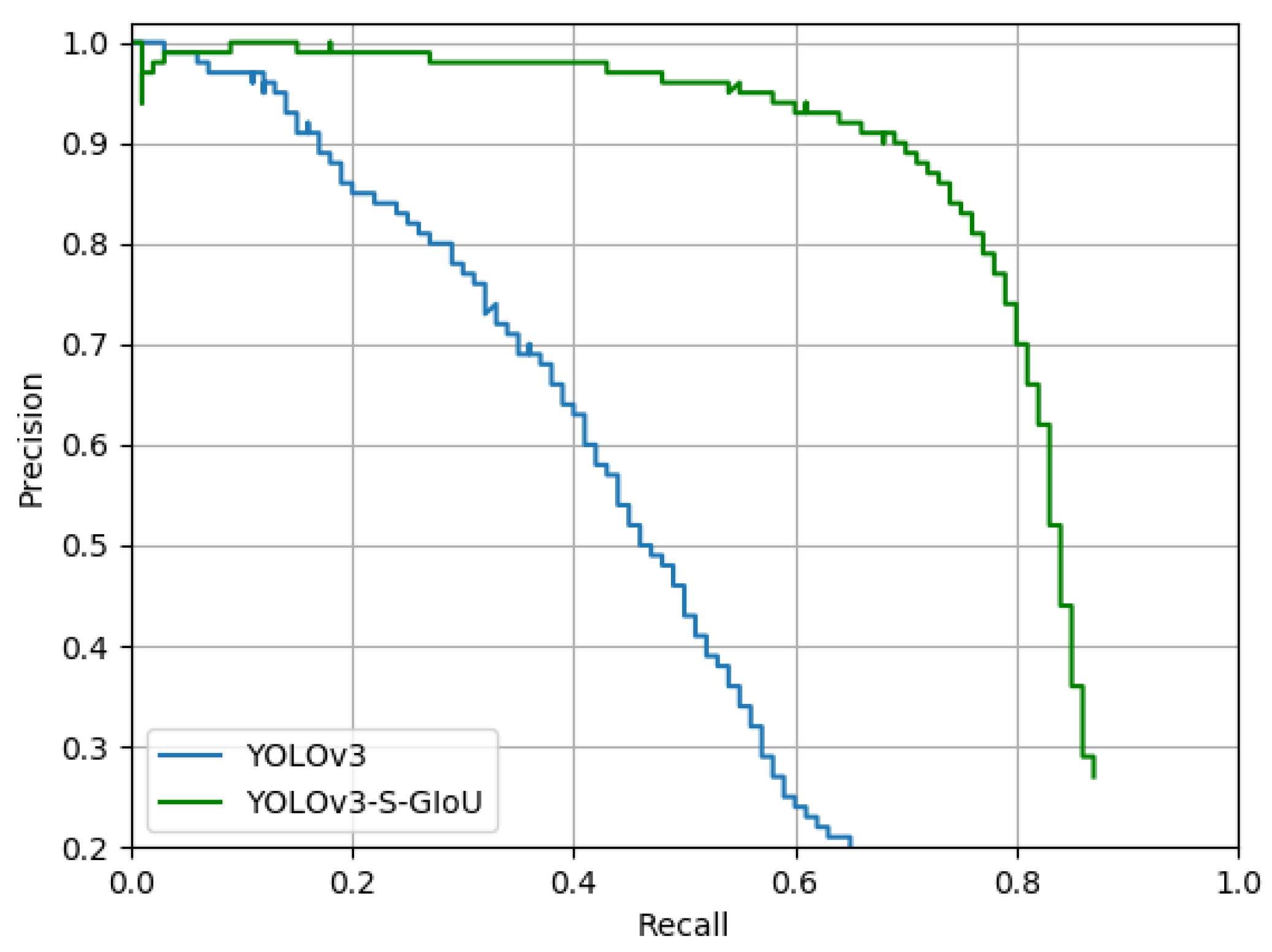
3.1.1. Precision Recall Curve

The precision recall curve is characterized by precision as the Y-axis and recall as the X-axis, such that before generating the PRC, we must calculate the precision and recall [32]. The equations for the precision, P, and recall rate, R, are as follows:
P = T P F P + T P ,
R = T P F N + T P ,
where TP, FP, and FN are listed in Table 2, i.e., the confusion matrix. Here, TP is the number of correctly detected positive samples, FP is the number of negative samples detected by error as positive samples, and FN is the number of positive samples not detected. If the area overlap ratio between the predicted bounding box and ground-truth bounding box is larger than 0.5, we set the predicted bounding box as a TP. Otherwise, it is set as a FP. Additionally, if several predicted bounding boxes overlap with the same ground-truth bounding box, only the box with a maximum overlap is regarded as a TP. The values of precision and recall rate have an inverse relationship.

3.1.2. Average Precision

As normally defined, the average precision refers to the average precision value within the interval from 0 to 1 for the recall rate, which is also the area under the precision recall curve. Normally, higher average precision results in better model performance. Currently, there are two methods to calculate the average precision: the first is to interpolate only 11 equidistant points and the second is to interpolate all the data points. In this study, we used the second method, i.e., the interpolation of all the data points using the following equation:
A P = R = 0 1 ( R n + 1 R n ) · P i n t e r p ( R n + 1 ) ,
P i n t e r p ( R n + 1 ) = max R ˜ : R ˜ R n + 1 P ( R ˜ ) ,
where P ( R ˜ ) represents the precision when the recall rate is R ˜ , and P i n t e r p ( R n + 1 ) is the maximum precision when the recall rate conforms to a certain condition, i.e., R ˜ R n + 1 .

3.1.3. F1 Score

The F1 score is used to evaluate the comprehensive performance of the model. The equation for calculating the F1 score is as follows:
F 1 = 2 P · R P + R .

3.1.4. FPS

FPS is a definition in the image field that refers to the number of frames transmitted per second. Higher FPS values result in more frames per second, yielding an increasingly smoother display. In this study, we used the FPS as an indicator of the algorithm processing speed, defined as the number of pictures processed per second in f/s. In general, real-time processing speed can be achieved when the FPS of the algorithm exceeds 30.

3.2. Implement Environment and Model Training
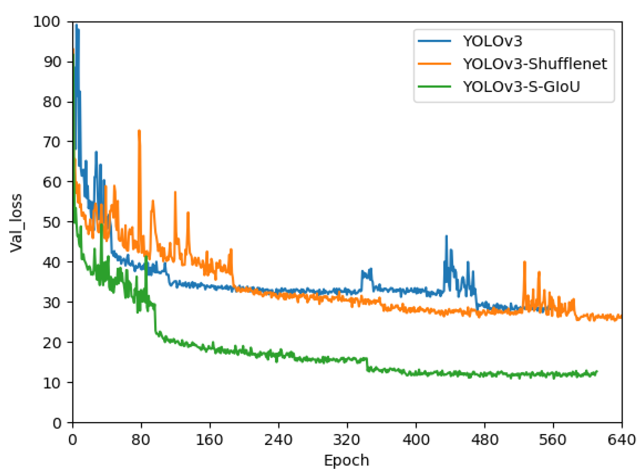
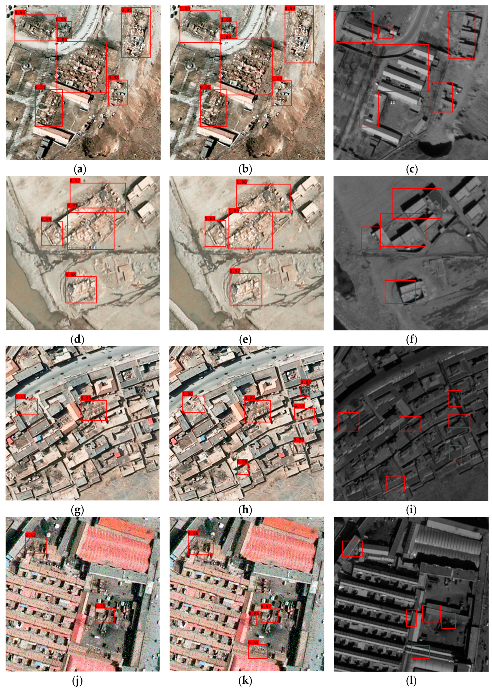
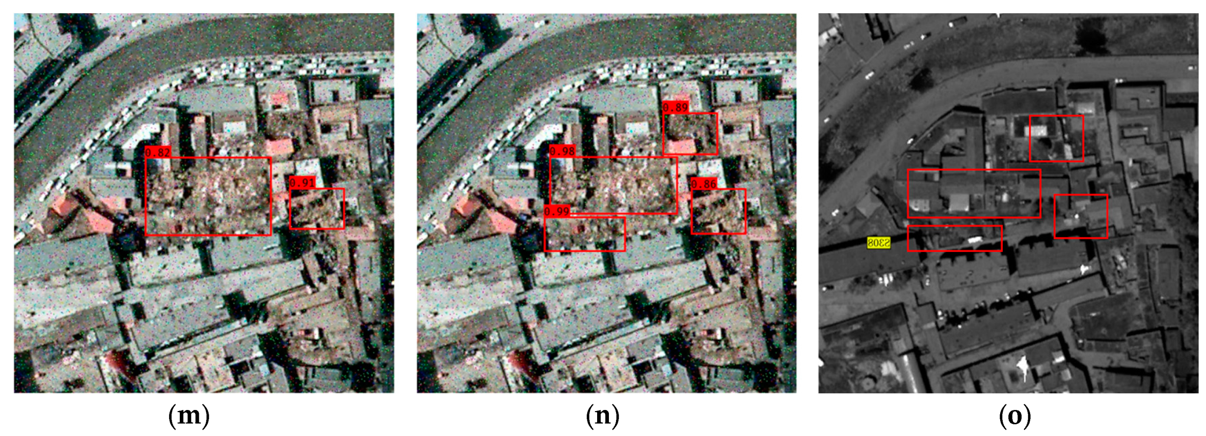
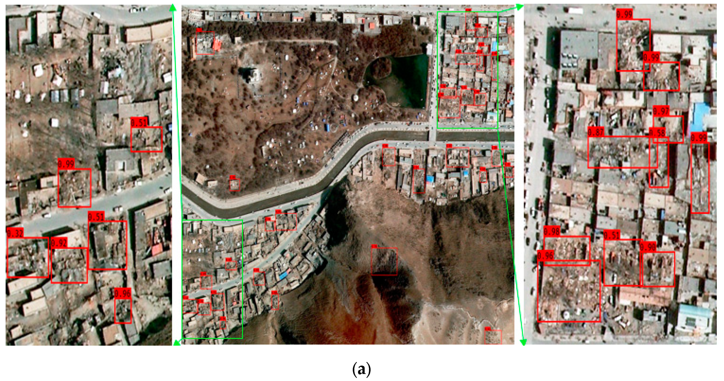
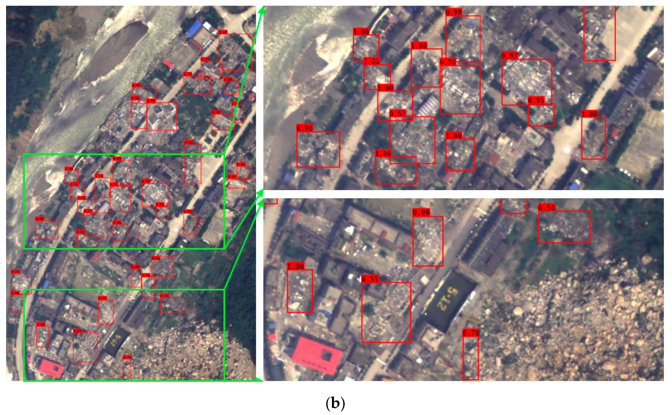
For this study, we used the following hardware environment for the experiment: an RTX2080Ti graphics, Intel i7-8700k processor, and 32 GB of memory.
For the model software environment both the original and improved YOLOv3 models were implemented with Keras, which is a high-level neural network API written in pure Python and backed by the TensorFlow or Theano deep learning libraries. TensorFlow was used as the backend for the Keras in this study. TensorFlow was developed by the Google Brain team as an open source software library for dataflow programming across a range of tasks.
In this study, the YOLOv3 network model, reproduced by the Keras, was first used for basic model training. Then, we used the ShuffleNet v2 network reproduced by the Keras to connect to the original YOLOv3 and replace the Darknet53 network. The new model was named the YOLOv3-ShuffleNet. Finally, based on the YOLOv3-ShuffleNet model, the XY loss and WH loss in the loss function were replaced by the GIoU loss, which was named the YOLOv3-S-GIoU. During the training process, the parameters were gradually optimized and adjusted. Finally, the optimizer was selected as Adam and the batch size was 8. The initial learning rate was set at 10−3. In the training process, if the loss value on the verification set did not decrease after 20 epochs (each epoch refers to the forward propagation of all training images), the learning rate should be reduced by 0.1-fold, where the lowest learning rate was 106. Finally, the original YOLOv3, improved YOLOv3-ShuffleNet, and YOLOv3-S-GIoU models were each trained for approximately 600 epochs.

4. Results

4.1. Quantitative Evaluation

The three models, i.e., YOLOv3, YOLOv3-ShuffleNet, and YOLOv3-S-GIoU, compared in this study were trained with the same dataset. Figure 12 shows their loss change curves for the validation set during training. The loss change curves for the validation set shows that the three models had both similarities and differences. First, the general trend in the three models was roughly the same, i.e., the loss value rapidly decreased during early training stages, with a large jitter range. This was due to a large learning rate in the early stage, which was able to produce a relatively fast learning speed and reduce the loss value to a relatively low point as soon as possible. In the middle and later stages of training, the learning rate gradually decreased, the change in the loss value tended to be stable, and the decline in the speed was much slower. Second, the loss curves for the three models also had several differences, i.e., the timing of the violent jitter for the YOLOv3-S-GIoU’s loss value during the early stage was shorter than that of the other two models, with a smaller jitter amplitude. The loss value was much lower than that of the other two models because the change in the loss function for the YOLOv3-S-GIoU caused a large change in the loss value.
After the training, the two improved models were compared with the original YOLOv3 model, whose results are listed in Table 3. The precision, P, and recall rate, R, in Table 3 were obtained by adjusting the threshold to maximize the F1 score. The final improved YOLOv3-S-GIoU model used in this study had a precision of 93%, a recall rate of 88%, an average precision of 90.89%, and an FPS of 29.23 f/s on the test set. Compared with the original YOLOv3 model, we significantly improved these parameters by 5, 10, 5.05, and 5.28 f/s, respectively. First, the improvement in precision and recall rate can be attributed to the improvement in the loss function. By replacing the center point loss and width and height loss of the prediction box in the loss function with the GIoU loss, we were able to more accurately evaluate the relationship between the prediction box and real box, such that we could accurately evaluate the loss of the prediction box relative to the real box. The loss function value decreased in a more accurate direction and the model precision was improved. Second, the improvement in the detection speed benefited from improvements to the network structure. The lightweight ShuffleNet v2 network replaced the basic Darknet53 convolutional network, which reduced the number of network parameters and improved the model’s running speed. Benefit from the clever design of the ShuffleNet v2 network, the network maintained high precision while reducing the number of parameters and increasing the speed.

4.2. PRC Evaluation

For the object detection method, the PRC is one of the basic indicators of robustness and effectiveness. Figure 13 shows the PRC of the three YOLOv3 models used in this study. We could observe based on the curve that, with an increase in the recall rate, there is a gradual decrease in the precision. When the recall rate was approximately 0.88, the precision of YOLOv3 and YOLOv3-ShuffleNet declined significantly to only approximately 0.6 but the precision for YOLOv3-S-GIoU remained at approximately 0.93. In other words, the precision of the improved model had clear advantages at an identical recall rate, which indicates that using the GIoU as the loss function could better and more fully train the model, as well as improve the model’s detection performance.
Based on the average confidence of the positive and negative samples during the training process, there was a slight increase in the confidence of the positive and negative samples in the YOLOv3-S-GIoU model. This increase enhanced the confidence of the positive samples, as well as yielding a good convergence effect. Based on the results in Figure 14a,b,d,e, we could also observe that, although the original YOLOv3 model could detect most collapsed buildings, the confidence of the test results was lower than that of the YOLOv3-S-GIoU model. In Figure 14g,h, the original YOLOv3 model missed numerous small targets. This all indicates that the YOLOv3-S-GIoU model was more fully trained and had a better convergence effect than the original YOLOv3 model.
To evaluate the model’s robustness and anti-noise ability, we randomly added Gaussian noise and salt-pepper noise into the test set for the original YOLOv3 and improved YOLOv3-S-GIoU models, respectively. The images after adding noise are shown in Figure 15, and the test results are shown in Table 4. The average precision of the original YOLOv3 model after adding noise was only 44.3% while the average precision of the improved YOLOv3-S-GIoU model remained high, reaching 79.8%.
Based on the PRC after the addition of noise in Figure 16, with an increase in the recall rate, there was rapid decrease in the precision of the original YOLOv3 model. When the recall rate was only 0.6, the precision was near 0. This indicates that the improved model has a stronger anti-noise ability than the original YOLOv3 model, i.e., the improved model has a stronger generalization ability. We could also observe from Figure 14j,k,m,n after adding the noise that numerous small targets could not be detected in the original YOLOv3 model. The analysis shows that the lightweight CNN like ShuffleNet v2 had better generalization and prevented over-fitting, whereas the number of parameters in Darknet53 for this study was too large, which may lead to over-fitting.
The improved YOLOv3-S-GIoU model in this study increased model precision by replacing the original loss function with a better GIoU loss function. Moreover, the lightweight CNN could be used to improve the model’s generalization ability, yielding excellent precision and generalization.
Figure 17 shows examples of the detection results for the YOLOv3-S-GIoU model in test remote sensing images. Figure 17a is a test image from the Yushu earthquake while Figure 17b is a test image from the Wenchuan earthquake. Based on the test results, the YOLOv3-S-GIoU model could detect most collapsed buildings in the remote sensing images but there were also certain cases of false and missed detections. This is mainly because the background environment in the high-resolution remote sensing images after the earthquake is far more complex than that in the natural image, which leads to the model’s detection of certain objects in the background environment as collapsed buildings. For example, bare soil with similar image characteristics of collapsed buildings is easy to be detected by mistake. In addition, the model easily misses certain collapsed buildings that are similar to the background image features.

5. Discussion

There have been several studies using remote sensing images to extract buildings that collapsed or were damaged after the 2008 Wenchuan earthquake and the 2010 Yushu earthquake. Zhao et al. used an object-oriented change detection method based on multiple classifiers to extract the information of building damage after the Yushu earthquake. When constructing the multi-classifier system, by means of multi-feature extraction, selection, and integration, random subspace recognition technology was used to integrate the limit learning machine model, multiple logistic regression model, and K nearest model, improving the performance of the multi-classifier system and the overall accuracy to 88.45% [33]. Wen et al. used LiDAR (light detection and ranging) data and high-resolution Quickbird remote sensing data in the Yushu disaster area, preprocessed the LiDAR data in the study area, and extracted the information of collapsed buildings after the earthquake using a method combining object-oriented classification and SVM technology. The total extraction accuracy was 82.21% [34]. Ji et al. extracted each building object from remote sensing images using building vector data, and then used CNN to classify buildings that had completely collapsed and buildings that were intact or less affected, with an average accuracy of 78.6% [22]. Of the above studies, most of them have achieved high accuracy, but the data used in these studies are more, such as pre-earthquake remote sensing images, LiDAR data, and building vector data. These data may not be obtained in time after the earthquake. In this study, we used the CNN-based object detection method YOLOv3 to detect collapsed buildings and obtained an ideal result with an accuracy of 90.89%, and our approach is more practical than that of previous studies. First, the YOLOv3 model only requires post-earthquake remote sensing images, thus, eliminating the trouble of obtaining pre-earthquake remote sensing images. Second, the YOLOv3 model can extract collapsed buildings without the aid of building vector data. Since it is often difficult to obtain building vector data in time after the earthquake, the use of building vector data has certain limitations in practical applications, which are addressed by YOLOv3.
In this study, certain measures were taken to prevent the over-fitting phenomenon when training the CNN. First, as the collected seismic data is relatively small, as well as the fact that it is necessary to screen out high spatial resolution data with a resolution of 1 m or less to better detect individual collapsed buildings, the data that conforms to the requirements is even less. These limited samples easily lead to over-fitting when they are used to train the large convolutional neural network in the training set. Therefore, the dataset was enhanced and expanded to increase the sample diversity. Second, in the YOLOv3 network structure, when using the Darknet53 convolutional neural network in this study to detect only a single class of objects appears to have too many parameters, which easily lead to over-fitting. Therefore, we proposed the replacement of Darknet53 with the lightweight CNN ShuffleNet v2 to significantly reduce the number of parameters and effectively improve the over-fitting situation. Finally, during the training process, when the value of the loss function is unable to decrease after 50 epochs, training was terminated in advance to avoid excessive learning.
In addition to the prevention of overfitting, the loss function in YOLOv3 was modified to improve the detection precision of damaged buildings. In the original YOLOv3 loss function, using the cross-entropy loss to predict the center point coordinates and width and height of the rectangular box is not reasonable. When the true value is 0 or 1, the cross-entropy loss can accurately evaluate the loss of the predicted value relative to the true value, whereas when the true value is between 0 and 1, the loss of the predicted value relative to the true value cannot be accurately evaluated. Therefore, the GIoU loss was used in this study to predict the center point coordinates and width and height of the rectangular boxes instead of the cross-entropy loss. As the GIoU can accurately describe the relationship between the prediction and true boxes, the GIoU can accurately evaluate the loss of the prediction box relative to the true box in the training process.

6. Conclusions

In this study, a dataset of collapsed buildings in remote sensing images was self-labeled using aerial remote sensing images after earthquakes. We then proposed the detection of the collapsed buildings in remote sensing images after earthquakes using the YOLOv3 deep learning object detection model, and the basic convolutional network framework and loss function of the YOLOv3 model were improved. The experimental results show that the improved YOLOv3 model (YOLOv3-S-GIoU) had sufficient robustness and a certain anti-noise ability when detecting collapsed buildings. While the speed within the test set reached 29.23 f/s, the average precision reached 90.89% and a significant reduction in the number of parameters, i.e., only 146 MB. This study verified the feasibility and effectiveness of the improved YOLOv3-S-GIoU model to detect collapsed buildings in high spatial resolution remote sensing images after earthquakes. However, due to the small amount of seismic data and certain errors in sample labeling due to a lack of ground survey data support, there were still some errors in the comparison between the test results and the ground truth. Therefore, to obtain a better detection effect and make the model more practical, extending the training dataset, including remote sensing images of different types and resolutions, is the future work to be tested for improvement.

Author Contributions

All authors contributed in a substantial way to the manuscript. H.M. conceived, designed and performed the research and wrote the manuscript. Y.L. and Y.R. made contributions to the design of the research and data analysis. All authors discussed the basic structure of the manuscript. All authors have read and agreed to the published version of the manuscript.

Funding

This research was funded by National Key Research and Development Program, Project NO. 2017YFC1500902.

Acknowledgments

The authors would like to thank the anonymous reviewers for their very competent comments and helpful suggestions.

Conflicts of Interest

The authors declare no conflict of interest.

References

  1. Dell’Acqua, F.; Gamba, P. Remote sensing and earthquake damage assessment: Experiences, limits, and perspectives. Proc. IEEE 2012, 100, 2876–2890. [Google Scholar] [CrossRef]
  2. Chen, W. Research of Remote Sensing Application Technology Based on Earthquake Disaster Assessment; China Earthquake Administration Lanzhou Institute of Seismology: Lanzhou, China, 2007. [Google Scholar]
  3. Cooner, A.; Shao, Y.; Campbell, J. Detection of urban damage using remote sensing and machine learning algorithms: Revisiting the 2010 Haiti earthquake. Remote Sens. 2016, 8, 868. [Google Scholar] [CrossRef] [Green Version]
  4. Uprety, P.; Yamazaki, F.; Dell’Acqua, F. Damage detection using high-resolution SAR imagery in the 2009 L’Aquila, Italy, Earthquake. Earthq. Spectra 2013, 29, 1521–1535. [Google Scholar] [CrossRef] [Green Version]
  5. Menderes, A.; Erener, A.; Sarp, G. Automatic detection of damaged buildings after earthquake hazard by using remote sensing and information technologies. Procedia Earth Planet. Sci. 2015, 15, 257–262. [Google Scholar] [CrossRef] [Green Version]
  6. Gong, L.; Li, Q.; Zhang, J. Earthquake building damage detection with object-oriented change detection. In Proceedings of the IEEE International Geoscience and Remote Sensing Symposium-IGARSS, Melbourne, Australia, 21–26 July 2013; pp. 3674–3677. [Google Scholar]
  7. Ye, X.; Wang, J.; Qin, Q. Damaged building detection based on GF-1 satellite remote sensing image: A case study for Nepal MS8.1 earthquake. Acta Seismol. Sin. 2016, 38, 477–485. [Google Scholar]
  8. Dong, L.; Shan, J. A comprehensive review of earthquake-induced building damage detection with remote sensing techniques. ISPRS J. Photogramm. Remote Sens. 2013, 84, 85–99. [Google Scholar] [CrossRef]
  9. Janalipour, M.; Mohammadzadeh, A. A fuzzy-ga based decision making system for detecting damaged buildings from high-spatial resolution optical images. Remote Sens. 2017, 9, 349. [Google Scholar] [CrossRef] [Green Version]
  10. Dai, W.; Jin, L.; Li, G. Real-time airplane detection algorithm in remote-sensing images based on improved YOLOv3. Opto Electron. Eng. 2018, 45, 84–92. [Google Scholar]
  11. Girshick, R.; Donahue, J.; Darrell, T. Rich feature hierarchies for accurate object detection and semantic segmentation. In Proceedings of the IEEE Conference on Computer Vision and Pattern Recognition, Columbus, OH, USA, 23–28 June 2014; pp. 580–587. [Google Scholar]
  12. Ren, S.; He, K.; Girshick, R. Faster R-CNN: Towards real-time object detection with region proposal networks. In Proceedings of the Annual Conference on Neural Information Processing Systems, Montreal, QC, Canada, 7–12 December 2015; pp. 91–99. [Google Scholar]
  13. He, K.; Gkioxari, G.; Dollár, P. Mask R-CNN. In Proceedings of the IEEE Conference on Computer Vision and Pattern Recognition, Honolulu, HI, USA, 21–26 July 2017; pp. 2961–2969. [Google Scholar]
  14. Redmon, J.; Divvala, S.; Girshick, R. You only look once: Unified, real-time object detection. In Proceedings of the IEEE Conference on Computer Vision and Pattern Recognition, Las Vegas, NV, USA, 27–30 June 2016; pp. 779–788. [Google Scholar]
  15. Liu, W.; Anguelov, D.; Erhan, D. SSD: Single shot multibox detector. In Proceedings of the European Conference on Computer Vision, Amsterdam, The Netherlands, 8–16 October 2016; pp. 21–37. [Google Scholar]
  16. Redmon, J.; Farhadi, A. YOLO9000: Better, faster, stronger. In Proceedings of the IEEE Conference on Computer Vision and Pattern Recognition, Honolulu, HI, USA, 21–26 July 2017; pp. 7263–7271. [Google Scholar]
  17. Redmon, J.; Farhadi, A. YOLOv3: An incremental improvement. arXiv 2018, arXiv:1804.02767. [Google Scholar]
  18. Han, X.; Zhong, Y.; Zhang, L. An efficient and robust integrated geospatial object detection framework for high spatial resolution remote sensing imagery. Remote Sens. 2017, 9, 666. [Google Scholar] [CrossRef] [Green Version]
  19. Cheng, G.; Zhou, P.; Han, J. Learning rotation-invariant convolutional neural networks for object detection in VHR optical remote sensing images. IEEE Trans. Geosci. Remote Sens. 2016, 54, 7405–7415. [Google Scholar] [CrossRef]
  20. Zheng, Z.; Liu, Y.; Pan, C. Application of improved YOLOv3 in aircraft recognition of remote sensing images. Electron. Opt. Control. 2019, 26, 32–36. [Google Scholar]
  21. Duarte, D.; Nex, F.; Kerle, N. Satellite image classification of building damages using airborne and satellite image samples in a deep learning approach. ISPRS Ann. Photogramm. Remote Sens. Spat. Inf. Sci. 2018, 4, 89–96. [Google Scholar] [CrossRef] [Green Version]
  22. Ji, M.; Liu, L.; Buchroithner, M. Identifying collapsed buildings using post-earthquake satellite imagery and convolutional neural networks: A case study of the 2010 Haiti earthquake. Remote Sens. 2018, 10, 1689. [Google Scholar] [CrossRef] [Green Version]
  23. Everingham, M.; Van Gool, L.; Williams, C.K.I.; Winn, J.; Zisserman, A. The PASCAL visual object classes (VOC) challenge. Int. J. Comput. Vis. 2010, 88, 303–338. [Google Scholar] [CrossRef] [Green Version]
  24. Perez, L.; Wang, J. The effectiveness of data augmentation in image classification using deep learning. arXiv 2017, arXiv:1712.04621. [Google Scholar]
  25. Ioffe, S.; Szegedy, C. Batch normalization: Accelerating deep network training by reducing internal covariate shift. arXiv 2015, arXiv:1502.03167. [Google Scholar]
  26. He, K.; Zhang, X.; Ren, S. Deep residual learning for image recognition. In Proceedings of the IEEE Conference on Computer Vision and Pattern Recognition, Seattle, WA, USA, 27–30 June 2016; pp. 770–778. [Google Scholar]
  27. Ma, N.; Zhang, X.; Zheng, H. ShuffleNet v2: Practical guidelines for efficient CNN architecture design. In Proceedings of the European Conference on Computer Vision, Munich, Germany, 8–14 September 2018; pp. 116–131. [Google Scholar]
  28. Chollet, F. Xception: Deep learning with depthwise separable convolutions. In Proceedings of the IEEE Conference on Computer Vision and Pattern Recognition, Honolulu, HI, USA, 21–26 July 2017; pp. 1800–1807. [Google Scholar]
  29. Zhang, X.; Zhou, X.; Lin, M. ShuffleNet: An extremely efficient convolutional neural network for mobile devices. In Proceedings of the IEEE Conference on Computer Vision and Pattern Recognition, Salt Lake City, UT, USA, 18–23 June 2018; pp. 6848–6856. [Google Scholar]
  30. Rezatofighi, H.; Tsoi, N.; Gwak, J.Y. Generalized intersection over union: A metric and a loss for bounding box regression. In Proceedings of the IEEE Conference on Computer Vision and Pattern Recognition, Los Angeles, CA, USA, 16–19 June 2019; pp. 658–666. [Google Scholar]
  31. Tian, Y.; Yang, G.; Wang, Z. Apple detection during different growth stages in orchards using the improved YOLO-V3 model. Comput. Electron. Agric. 2019, 157, 417–426. [Google Scholar] [CrossRef]
  32. Benjdira, B.; Khursheed, T.; Koubaa, A. Car detection using unmanned aerial vehicles: Comparison between Faster R-CNN and YOLOv3. In Proceedings of the International Conference on Unmanned Vehicle Systems-Oman (UVS), Sultan Qaboos Univ, Muscat, Oman, 5–7 February 2019; pp. 1–6. [Google Scholar]
  33. Zhao, Y.; Ren, H.; Cao, D. The research of building earthquake damage object-oriented change detection based on ensemble classifier with remote sensing image. In Proceedings of the IEEE International Geoscience and Remote Sensing Symposium-IGARSS, Valencia, Spain, 22–27 July 2018; pp. 4950–4953. [Google Scholar]
  34. Wen, X.; Bi, X.; Xiang, W. Object-oriented collapsed building extraction from multi-source remote sensing imagery based on SVM. North China Earthq. Sci. 2015, 33, 13–19. [Google Scholar]
Figure 1. Location of the study area.
Remotesensing 12 00044 g001
Figure 2. Labeled samples of collapsed buildings. The green rectangles in (a,b) are collapsed buildings.
Remotesensing 12 00044 g002
Figure 3. Image enhancement methods: (a) original image, (b) 90-degree rotation, (c) 180-degree rotation, (d) 270-degree rotation, (e) horizontal flip, (f) up-and-down flip, (g) color transformation, and (h) image stretching.
Remotesensing 12 00044 g003
Figure 4. Method flow chart.
Remotesensing 12 00044 g004
Figure 5. YOLOv3 network structure, where the blue and red lines represent two-fold up-sampling.
Remotesensing 12 00044 g005
Figure 6. Schematic of the YOLOv3 prediction bounding box with 13 cells × 13 cells. (a) YOLOv3 detection process on 13 cells × 13 cells feature map; (b) YOLOv3 detection result.
Remotesensing 12 00044 g006
Figure 7. Structure of the Darknet53 convolutional network.
Remotesensing 12 00044 g007
Figure 8. Basic units of the ShuffleNet (DWConv: depth-wise convolution; GConv: group convolution): (a) basic unit of ShuffleNet v1, (b) basic unit for scaling down in ShuffleNet v1, (c) basic unit of ShuffleNet v2, and (d) basic unit for scaling down in ShuffleNet v2.
Remotesensing 12 00044 g008
Figure 9. ShuffleNet v2 network structure
Remotesensing 12 00044 g009
Figure 10. Sigmoid function and its derivative.
Remotesensing 12 00044 g010
Figure 11. Three different overlapping situations for two rectangular boxes.
Remotesensing 12 00044 g011
Figure 12. Loss curves on the verification set of three YOLOv3 models.
Remotesensing 12 00044 g012
Figure 13. Comparison of the precision recall curves for the three YOLOv3 models for YOLOv3 in blue, YOLOv3-ShuffleNet in red, and YOLOv3-S-GIoU in green.
Remotesensing 12 00044 g013
Figure 14. Comparison of detection results of between the original YOLOv3 and YOLOv3-S-GIoU. The first column represents the original YOLOv3 detection results; the second column represents the YOLOv3-S-GIoU detection results; the third column denotes the images before the earthquake. (a,b,d,e,g,h) are the detection results of the images without adding noise; (j,k,m,n) are the detection results of the images after adding noise.
Remotesensing 12 00044 g014aRemotesensing 12 00044 g014b
Figure 15. Images with noise: (a) original image, (b) image with Gaussian noise, and (c) image with salt-pepper noise.
Remotesensing 12 00044 g015
Figure 16. Comparison of the precision recall curves for the two YOLOv3 models after the addition of noise to the test set.
Remotesensing 12 00044 g016
Figure 17. Example of YOLOv3-S-GIoU model detection results. (a) Test image for the Yushu earthquake; (b) test image for the Wenchuan earthquake
Remotesensing 12 00044 g017aRemotesensing 12 00044 g017b
Table 1. The dataset division.
Number of Sample ImagesNumber of Collapsed Buildings
Training set14568751
Validation set3642516
Testing set3602234
Table 2. Confusion matrix for predicted results and ground truth.
Ground Truth
Collapsed BuildingOthers
Collapsed buildingTrue Positive (TP)False Positive (FP)
OthersFalse Negative (FN)True Negative (TN)
Table 3. Performance comparison between YOLOv3 and the two improved models.
P (%)R (%)F1 (%)AP (%)FPS (f/s)Parameter Size (M)
YOLOv3887882.785.8423.95241
YOLOv3-ShuffleNet878183.8985.9829.16146
YOLOv3-S-GIoU938890.4390.8929.23146
Table 4. Performance comparison of the two YOLOv3 models after the addition of noise.
P (%)R (%)F1 (%)AP (%)
YOLOv3634149.6744.3
YOLOv3-S-GIoU867479.5579.8

