Matching Confidence Constrained Bundle Adjustment for Multi-View High-Resolution Satellite Images

Abstract

Bundle adjustment of multi-view satellite images is a powerful tool to align the orientations of all the images in a unified framework. However, the traditional bundle adjustment process faces a problem in detecting mismatches and evaluating low/medium/high-accuracy matches, which limits the final bundle adjustment accuracy, especially when the mismatches are several times more than the correct matches. To achieve more accurate bundle adjustment results, this paper formulates the prior knowledge of matching accuracy as matching confidences and proposes a matching confidence based bundle adjustment method. The core algorithm firstly selects several highest-confidence matches to initially correct orientations of all images, then detects and eliminates the mismatches under the initial orientation guesses and finally formulates both the matching confidences and the forward-backward projection errors as weights in an iterative bundle adjustment process for more accurate orientation results. We compared our proposed method with the famous RANSAC strategy as well as a state-of-the-art bundle adjustment method on the high-resolution multi-view satellite images. The experimental comparisons are evaluated by image checking points and ground control points, which shows that our proposed method is able to obtain more robust and more accurate mismatch detection results than the RANSAC strategy, even though the mismatches are four times more than the correct matches and it can also achieve more accurate orientation results than the state-of-the-art bundle adjustment method.

1. Introduction

Given multi-view matches, the bundle adjustment (BA) of multi-view satellite images is to align the positions and attitudes of their cameras so that the optical rays from the corresponding pixels intersect at the same ground point in the object space. Its characteristics of high positioning accuracy have fueled many applications in photogrammetry and remote sensing, for example, digital surface model (DSM) generation [1], image registration [2], survey mapping [3] and so forth. The BA accuracy actually depend on the matching accuracy. Higher-accuracy matches normally result in higher-accuracy BA results and vice versa. An intuitive idea is to increase the contributions/weights of high-accuracy matches and decrease the contributions/weights of low-accuracy matches in the BA process for more accurate BA results. Therefore, the prior knowledge about the accuracy of each match is essential before BA.

The prior knowledge of the matching accuracy is normally assessed by measuring the geometric fitness between the matches and the orientation parameters (camera positions and attitudes) of satellite images. Most works [4,5,6,7] define the geometric fitness as the forward-backward projection errors (also called re-projection errors) in the image space. Smaller re-projection errors normally reflect higher matching accuracy and vice versa. However, the original orientation parameters of satellite images are of low positioning accuracy, for example, WorldView-3 with 5 m positioning errors [8], Gaofen-2 with 30 m positioning errors [9], thus bringing significant errors in the assessment of the matching accuracy. Therefore, some good matches are needed to correct the orientation parameters, while the assessment of good matches depends on the correct orientation parameters. Therefore, the assessments of good matches and the corrections of orientation parameters seem to be a chicken-or-egg issue.

To solve the aforementioned issue, an initial clue (either the good matches or the good guess of the orientation parameters) should be firstly given. Therefore, the BA methods can be categorized into—(1) the good match first methods, (2) the good orientation first methods and (3) the combined BA methods.

The good match first methods focus on firstly selecting good matches and then computing the accurate orientation parameters through the BA techniques [10,11,12,13]. The good matches are normally detected by using a random sample consensus (RANSAC) strategy with three steps—(1) randomly select minimum matches for the BA solutions; (2) compute orientation parameters using the selected matches and count the number of good matches/inliers whose re-projection errors under the orientation parameters are small (e.g., <1 pixel); (3) the process is iterated on until the maximum number of inliers is found and the corresponding inliers are used as the final good matches for BA. To give more robust good match predictions, some works improved RANSAC by integrating Graph-Cut [14] or “Random Grids” range-search technique [15] into the framework. The efficiency of RANSAC actually depends on the size of the minimum random samples. Large sample set size will significantly reduce the RANSAC efficiency. Therefore, the RANSAC strategy is often used in the pairwise corresponding pixels instead of the multi-view matches so that the minimum sample set size can be reduced to at least one. However, the RANSAC for pairwise correspondences cannot detect the mismatches along the epipolar lines, which will bring uncertainties in the good match selection results.

The good orientation first methods [6,7,16,17,18,19] normally obtain good orientation parameters using all matches in an iterative manner—(1) it firstly assumes equal/different contributions of all matches depending on prior knowledge and corrects the orientation parameters in the initial iteration; (2) then adjusts the weights of each match according to a certain mathematical model (e.g., inverse proportional model [6], t-distribution model [16] and exponential model [19]) under the orientation parameters of the previous iterations; (3) the process is iterated on until the iteration stopping criterion is satisfied. Such methods often formulate the re-projection errors as the geometric weights in BA so that they are able to decrease the contributions of mismatches and increase the contributions of good matches in multi-view scenarios. However, the orientation results in the previous iteration may be not reliable for adjusting the weights of the matches in the next iteration, when the mismatches are much more than the good matches (e.g., two times).

To achieve more robust BA results, especially when the mismatches are several times more than the good matches, several works combined the good match first methods and the good orientation first methods in a sequential workflow [4,5,20,21,22]—they firstly use the good match first methods to eliminate the majority of mismatches and then use the good orientation first methods to reduce the weights of the remaining mismatches for robust BA results. However, such methods often have troubles in exactly adjusting the weights of the good matches. For example, if half matches have 0 pixel matching errors and the remaining matches have 1 pixel matching errors, the theoretical orientation accuracy is about 0.5 pixels, which will assign equal weights to the 0 pixel accuracy matches and the 1 pixel accuracy matches during the BA process. To achieve more accurate BA results, it is essential to assign higher weights to higher-accuracy matches and vice versa.

In addition to the geometric fitness between the matches and the orientation parameters, an alternative way to predict the matching accuracy is the matching confidence [23,24,25,26,27], which normally reflects the significance of the matches when compared with the matching results of their surrounding pixels. Higher matching confidence often means higher possibilities of accurate matches and vice versa. However, all matching confidence studies only utilized the matching confidences in stereo dense matching with epipolar pairs instead of multi-view feature matching with unrectified images.

To achieve more accurate BA results, this paper improves the matching confidence metrics so that they can be applied in multi-view feature matching scenarios and formulates both the re-projection errors and the matching confidences as weights in the BA process. The core algorithm follows a sequential workflow of (1) good match selection and (2) iterative BA with the combined weights. For the first step, this paper firstly selects the highest-confidence matches for computing a good initial guess of the orientation parameters and then selects good matches whose re-projections errors under the good orientation parameters are small (<1 pixel). On the other hand, the matching confidences and the re-projection errors are respectively formulated as image weights and inverse proportional model based geometric weights in BA. We combine the both weights in BA process for more accurate BA results. The main contributions of our works include:

• We improve the matching confidence metrics so that they can be applied in multi-view feature matching scenarios, which can give helpful prior knowledge of the matching accuracy;
• A new matching confidence based mismatch detection algorithm is proposed, which can give a robust match selection result, even though the mismatches are several times more than the correct matches.
• A new weighting strategy by combining the geometric weight and the image weight in BA is proposed. It is the first time to formulate the matching confidences as weights in the BA of multi-view satellite images, which can improve the accuracy of BA results when compared with the state-of-the-art BA process.

The rest of the paper is organized as follows—Section 2 describes the methodology of the proposed method in detail; Section 3 shows the experimental results; and Section 4 concludes the manuscript.

2. Methodology

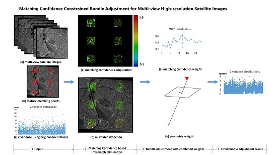
2.1. Workflow

To achieve accurate BA results, especially in the case of large amounts of mismatches, this paper formulates the prior knowledge of matching accuracy as different matching confidence metrics and proposes a matching confidence based BA method, which is able to remove large amounts of mismatches and adaptively adjust the weights of good matches in BA. The inputs of our work are multi-view satellite images with corresponding original orientation parameters (normally rational polynomial coefficients, RPC) and multi-view matches. In general, our work follows a sequential workflow with two steps—(1) matching confidence based mismatch elimination and (2) iterative BA with the combined weights. For the first step, we firstly compute the matching confidences for each match, then select highest-confidence matches for initial orientation parameter correction, and finally detect and eliminate mismatches using the corrected orientation parameters. Since it may run into the case that a few mismatches also have high matching confidences, we adopt inverse proportional model based geometric weights in the initial orientation corrections, which is able to reduce the weights of mismatches. For the second step, we formulate the matching confidences and the re-projection errors as image weights and inverse proportional model based geometric weights in BA and combine both weights to achieve more accurate BA results in an iterative manner. The workflow of our work is shown in Figure 1. In this paper, we firstly introduce several matching confidence metrics in Section 2.2, then describe a new matching confidence based mismatch elimination method in Section 2.3 and finally derive a new BA weighting strategy in Section 2.4.

2.2. Improved Matching Confidences for Feature Matching

Matching confidences measure the significance of each match among the matching results of its surrounding pixels. Higher matching confidence often means less uncertainties in the matching results, thus representing higher matching accuracy. Most works [23,24,25,26,27] only focused on applying the matching confidence in stereo dense image matching, where a pair of the original images is firstly rectified into the epipolar images and the confidence score of each two-view correspondence is measured along the 1D epipolar lines. To assess the prior accuracy of multi-view feature matching, this paper develops the matching confidence metrics in the multi-view matches from the unrectified original images, where the significance of each match is compared with its surrounding pixels in 2D image space. In general, we break the matching confidence of multi-view matches into the sub-confidences of pairwise two-view correspondences. For each two-view correspondence $\{\mathit{p},{\mathit{p}}^{\prime }\}$, we fix any one of the points (e.g., $\mathit{p}$), then compute ZNCC values between $\mathit{p}$ and the pixels in the searching window centered at ${\mathit{p}}^{\prime }$ and finally compute the matching confidence of $\{\mathit{p},{\mathit{p}}^{\prime }\}$ by comparing the ZNCC of $\{\mathit{p},{\mathit{p}}^{\prime }\}$ with all other ZNCCs in the searching window, as shown in Figure 2. Figure 2 shows the ZNCC values of all pixels in the searching window, which forms a curved surface. However, the matching of $\{\mathit{p},{\mathit{p}}^{\prime }\}$ may suffer from some geometric distortions (e.g., scale, rotation), which reduces the accuracy of the matching confidence evaluation. To reduce these geometric distortions, we resample all satellite images by projecting them on a common height plane before the matching confidence computation [28].

Matching results in textured regions are often reliable and the corresponding ZNCC curved surface in Figure 2a has an obvious peak (the maximum ZNCC value). On the other hand, matching results in untextured/weak-textured regions often contain high matching uncertainties and the corresponding ZNCC curved surface in (b) tends to be flat. Therefore, the shapes of the ZNCC curved surfaces can be used to predict matching accuracy. In this paper, we formulate the shape of the ZNCC curved surface as matching confidences. There are various matching confidence metrics to describe the shape, for example, the number of peaks, the highest peak values, the slope of the highest peaks, and so forth. According to Park and Yoon [23,24], Hu and Mordohai [25], and Egnal and Wildes [26,27]’s works of matching confidences in stereo epipolar image space, we totally select seven outstanding matching confidences which rank top among all matching confidence metrics and then we improve these metrics so that they can be applied for feature matching in unrectified original image space. It is possible that some matching confidences, which perform well in epipolar image space, may not obtain satisfying performances in the unrectified original image space. Therefore, we will analyze the performances of these matching confidence metrics in Section 3.1.

To simplify the formula of the matching confidence metrics in this paper, some basic notations are defined. $\mathit{m}=\{\mathit{p},{\mathit{p}}^{\prime }\}$ means a two-view correspondence between a image pair with $\mathit{p}=(x,y)$ in the left image and ${\mathit{p}}^{\prime }=(x^{\prime },y^{\prime })$ in the right image. $\mathit{d}=(dx,dy)$ means an offset from the center pixel. $C(\mathit{p},\mathit{q})$ is the ZNCC value between any two pixels $\mathit{p}$ in the left and $\mathit{q}$ in the right. $c_m$ means the ZNCC value of the correspondence itself. $\left\{C(\mathit{p},{\mathit{p}}^{\prime }+\mathit{d})\right|\mathit{d}\in D\}$ is the set of the ZNCC values, where D is the set of discrete offset vector from the center pixel in the searching window. We use ${\mathit{d}}_{\mathit{k}}$ to describe the offset vector of the kth maximum ZNCC value. For example, the offset vector of the maximum ZNCC value ${\mathit{d}}_{\mathbf{1}}$ are computed as ${\mathit{d}}_{\mathbf{1}}=\underset{\mathit{d}\in D}{argmax}(C(\mathit{p},{\mathit{p}}^{\prime }+\mathit{d}))$. Basically, the ZNCC values and offset vectors are computed with respect to the left image. We use the superscript${}^R$, when the ZNCC value or offset vector is computed with respect to the right image, for example, ${\mathit{d}}_{\mathbf{1}}^R=\underset{\mathit{d}\in D}{argmax}(C({\mathit{p}}^{\prime },\mathit{p}+\mathit{d}))$. $\mathit{W}(\mathit{p})=\left\{\mathit{p}+\mathit{d}\right|\mathit{d}\in \mathit{D}\}$ means the searching window centered at $\mathit{p}$.

In general, we use the peak height and the surface sharpness to describe the shape of the ZNCC curved surface and formulate these shape descriptors as matching confidence metrics. We also measure matching result consistencies between the correspondence and its surrounding pixels and formulate these consistencies as matching confidence metrics.

(a) the peak height

The ZNCC value of the correspondence itself is used to measure the peak height in the ZNCC curved surface. In textured regions, higher peaks/ZNCC values often represent higher matching accuracy. Therefore, the ZNCC metric can be used as a matching confidence metric:

$$f_{ZNCC}(\mathit{m})=c_m=C(\mathit{p},{\mathit{p}}^{\prime }).$$

(1)

The ZNCC metric defines the matching of $\mathit{p},{\mathit{p}}^{\prime }$ as the intensity correlations of their matching windows. In addition to ZNCC, our proposed method is also general to other matching cost metrics, for example, intensity differences, census [29] and the histogram of gradients (HOG) [30]. Some matching cost metrics prefer the maximum values (also called the-maximum-the-best metric), for example, ZNCC and some matching cost metrics prefer the minimum values (also called the-minimum-the-best metric), for example, census. Since our proposed method used ZNCC as an example metric in the matching confidence computation, it can be directly applied for all the-maximum-the-best metrics. For the-minimum-the-best metrics, the matching confidence equations in the paper can be simply changed by only subtracting all cost values c with the maximum of these cost values, in which case the matching confidence is used to describe the troughs of the curved surface.

(b) the surface sharpness

Sharper surfaces normally represent less matching uncertainties, thus leading to higher matching accuracy. Inspired by Park and Yoon’ works [23,24], we formulate the sharpness of the surface as (1) the differences of ZNCC values between the correspondence and its neighbor pixels, also termed as the local curvature (LC), (2) the maximum likelihood of the correspondence (ML) and (3) the attainable maximum likelihood of the correspondence (AML).

LC:

The local curvature (LC) metric computes the significance of the correspondence by comparing the ZNCC values of the correspondence with its neighborhoods on the ZNCC curved surface:

$$f_{LC}(\mathit{m})=8c_m-\sum _{\mathit{k}\in \mathit{N}(p^{\prime })}C(\mathit{p},\mathit{k}),$$

(2)

where $\mathit{N}(p^{\prime })$ is the eight neighborhood pixels of the pixel $p^{\prime }$.

ML:

The ZNCC values can be further considered as a probability density function and the correspondence should have the maximum likelihood:

$$f_{ML}(\mathit{m})=\frac{exp(-\frac{{(1-c_m)}^2}{2{\sigma }^2})}{{\sum }_{k\in \mathit{W}(p^{\prime })}exp(-\frac{{(1-c_k)}^2}{2{\sigma }^2})},$$

(3)

where $c_k=C(p,k)$ and $\sigma$ is a control parameter, which is formulated as the standard deviation of the ZNCC value. Too small $\sigma$ will decrease the probability of the high ZNCC values and the too large $\sigma$ will increase the probability of the low ZNCC values. In this paper, we empirically define $\sigma$ as 0.43.

AML:

Similar to ML, the ZNCC values can be defined as the attainable maximum likelihood (AML), as follows. When $c_m$ is dominant among all other ZNCC values, the denominator in Equation (4) is small, thus achieving high AML. Otherwise, the large denominator will lead to low AML.

$$f_{AML}(\mathit{m})=\frac{1}{{\sum }_{k\in \mathit{W}(p^{\prime })}exp(-\frac{{(c_m-c_k)}^2}{2{\sigma }^2})}.$$

(4)

(c) the consistency of the matching results

The above four matching confidence metrics rely on the shape of the ZNCC curved surface. An alternative way of measuring the matching confidence is to check the consistency between the matching results with respect to the left and the right images, also termed as left-right consistency (LRC) or the consistency between the matching results of the correspondence and its surrounding pixels, for example, the matching results of the correspondence should be similar to the median deviation (MDD) or mean deviation (MND) of the matching results of the surrounding pixels.

LRC:

$$f_{LRC}(\mathit{m})=-\frac{\left|\right|{\mathit{d}}_{\mathbf{1}}\left|\right|+\left|\right|{\mathit{d}}_{\mathbf{1}}^R\left|\right|}{2},$$

(5)

where $\left|\right|·\left|\right|$ is the normal of a vector. Smaller norms of the offset vectors mean more consistencies between the matching results with respect to the left images and the right images, thus bringing higher matching confidences.

MND:

MND is to compare the matching result of $\{\mathit{p},{\mathit{p}}^{\prime }\}$ with the average matching results of the surrounding pixels in the searching window. In this paper, we take the pixels $\mathit{W}(\mathit{p})=\{\mathit{p}+{\mathit{d}}_l|{\mathit{d}}_l\in \mathit{D}\}$ in the searching window of the left image as the basis and find their corresponding pixels in the right images. We firstly predict the initial positions of the corresponding pixels by setting the same offset as the basis pixels in the left image, as ${\mathit{p}}^{\prime }+{\mathit{d}}_l$, then find the more accurate corresponding pixels in the searching window centered at ${\mathit{p}}^{\prime }+{\mathit{d}}_l$ and finally compute the offset between the initial positions and the more accurate positions, as shown in Equation (6).

$$f_{MND}(\mathit{m})=-\frac{1}{\left|D\right|}\sum _{{\mathit{d}}_l\in \mathit{D}}\left|\right|\underset{d_r\in \mathit{D}}{argmax}(C(\mathit{p}+{\mathit{d}}_{\mathit{l}},({\mathit{p}}^{\prime }+{\mathit{d}}_l)+{\mathit{d}}_r)\left|\right|,$$

(6)

where $\left|D\right|$ is the number of offset vectors in the set D. ${\mathit{d}}_l$ is the offset from the center pixel $\mathit{p}$ and ${\mathit{d}}_r$ is the offset from the center pixel ${\mathit{p}}^{\prime }+{\mathit{d}}_l$. High MND means the matching results of $\{\mathit{p},{\mathit{p}}^{\prime }\}$ is similar to the average matching results of the surrounding pixel and vice versa.

MDD:

In addition to MND, the median deviation (MDD) of the matching results of the surrounding pixels can also be used to measure matching confidences:

$$f_{MDD}(\mathit{m})=-\underset{{\mathit{d}}_l\in \mathit{D}}{MED}\left(\left|\right|\underset{d_r\in \mathit{D}}{argmax}(C(\mathit{p}+{\mathit{d}}_{\mathit{l}},({\mathit{p}}^{\prime }+{\mathit{d}}_l)+{\mathit{d}}_r)\left|\right|\right).$$

(7)

These seven matching confidence metrics construct a seven-dimensional feature vector for the two-view correspondence $\mathit{m}$,

$$\mathit{f}(\mathit{m})=[f_{ZNCC},f_{LC},f_{ML},f_{AML},f_{LRC},f_{MND},f_{MDD}],$$

(8)

where the subscript of each element indicates the names of matching confidence metrics and $\mathit{m}$ is omitted in each element since it is the same for all elements and is already noted in the left side of Equation (8). In Section 3.1, we will analyse the performance of these matching confidence metrics in multi-view feature matching cases and select the top N important confidence measures to construct a more reliable feature vector:

$$\widehat{\mathit{f}}(\mathit{m})=[\overline{f_1},\overline{f_2},\cdots ,\overline{f_N}],$$

(9)

where the subscript of each element indicates its importance in predicting matching accuracy, for example, $f_1$ is the most important matching confidence metric. $\overline{f_i}$ is the normalized matching confidence metric. Since the scales of each matching confidence metric may be different (e.g., LC and ZNCC), all matching confidence metrics in Equation (9) need to be respectively normalized so that these normalized confidences can make equal contributions to the final matching confidence score of $\mathit{m}$. Then, we compute the first-order norm of the N-dimensional feature vector $\widehat{\mathit{f}}(\mathit{m})$ as the final matching confidence score for $\mathit{m}$.

After computing the final matching confidence score for each two-view correspondence, we need to merge these correspondences as well as their two-view matching confidence scores across the multi-view images to generate the matching confidences of the multi-view matches, as shown in Equation (10).

$$\mathit{F}({\mathit{M}}_{\mathit{j}})=\sum _{{\mathit{m}}_{i,i^{\prime }}\in {\mathit{M}}_j}S({\mathit{m}}_{i,i^{\prime }})/{\mathrm{C}}_{|{\mathit{M}}_j|}^2,$$

(10)

where ${\mathit{M}}_j$ is the jth multi-view matches; ${\mathit{m}}_{i,i^{\prime }}$ is the two-view correspondence of ${\mathit{M}}_j$ on the image i and $i^{\prime }$; $S({\mathit{m}}_{i,i^{\prime }})$ is the final confidence score of the two-view correspondence ${\mathit{m}}_{i,i^{\prime }}$, which is computed by averaging the absolute elements in Equation (9); $|{\mathit{M}}_j|$ is the number of the multi-view connectivity of ${\mathit{M}}_j$; $F({\mathit{M}}_j)$ is the matching confidence score of the match ${\mathit{M}}_j$.

2.3. Matching Confidence Based Mismatch Elimination

Given a multi-view satellite image set $I=\{I_1,I_2,\cdots ,I_n\}$ with n being the image number, the original orientation parameters (e.g., RPCs in this paper), the multi-view matches $\mathit{M}=\{{\mathit{M}}_{\mathbf{1}},{\mathit{M}}_{\mathbf{2}},\cdots ,{\mathit{M}}_{\mathit{t}}\}$ with t being the matches number and their corresponding matching confidence scores $\mathit{F}=\{F({\mathit{M}}_{\mathbf{1}}),F({\mathit{M}}_{\mathbf{2}}),\cdots ,F({\mathit{M}}_{\mathit{t}})\}$, we develop a confidence based mismatch elimination method with three steps—(1) highest-confidence matches selection, which selects a certain percentage of the highest-confidence matches; (2) initial orientation correction, which uses these highest-confidence matches to correct the RPCs of all satellite images through an iterated BA technique with inverse proportional model based geometric weights [6,7]; (3) mismatch elimination, which computes the re-projection errors of all matches using the corrected orientations and finally eliminates the mismatches whose re-projection errors are larger than a given threshold (e.g., 1 pixel in this paper) so that the BA result is guaranteed to be better than 1 pixel, which will meet the requirement of the remote sensing applications.

2.3.1. Highest-Confidence Matches Selection

The matches with the highest matching confidences often have the highest possibilities of being correct. Therefore, we select a certain percentage $a\%$ (e.g., a = 1) of the highest-confidence matches in our proposed method. To guarantee that each image has enough matches in the later initial orientation corrections, we break the selection from all multi-view matches into the ones from pairwise correspondences and then merge these pairwise highest-confidence correspondences into the multi-view matches, as shown in Equation (11).

$${\mathit{M}}_H=\bigcup _{i,j\in \mathit{I}}\left\{{\mathit{m}}_{\mathit{v}}\right|{\mathit{m}}_{\mathit{v}}\in {\mathit{M}}_{i,j}·a\%\wedge {\mathit{n}}_{\mathit{v}}\in (\mathit{M}-{\mathit{M}}_{i,j}·a\%)\wedge F({\mathit{m}}_{\mathit{v}})>F({\mathit{n}}_{\mathit{v}})\},$$

(11)

where ${\mathit{M}}_H$ is the highest-confidence match set of $\mathit{M}$; ${\mathit{M}}_{i,j}$ is the match set that has corresponding pixels on the image pair $\{i,j\}$; ${\mathit{m}}_{\mathit{v}}$ is a multi-view match within the top $a\%$ highest-confidence matches; ${\mathit{M}}_{i,j}·a\%$ is a sub-set of ${\mathit{M}}_{i,j}$ with element number being $|{\mathit{M}}_{i,j}|·a\%$; $\mathit{M}-{\mathit{M}}_{i,j}·a\%$ is a complementary set of ${\mathit{M}}_{i,j}·a\%$; $n_v$ is a match in $\mathit{M}-{\mathit{M}}_{i,j}·a\%$.

Our goal is to select the matches with the highest possibilities of being correct in the mismatch elimination process. Therefore, we only consider matching confidences in the matches selection, except for the distributions and the multi-view connectivity of the matches, both of which will decrease the contributions of the matching confidences in the matches selection. These highest- confidence matches can be used to initially correct orientation parameters of satellite images for the mismatch elimination.

2.3.2. Initial Orientation Correction

The highest-confidence matches are used to initially correct orientation parameters of multi-view satellite images, while it is still possible that a few mismatches with high matching confidences are selected. Therefore, we adopt a geometric weighting strategy in the initial orientation correction, which is able to decrease the weights of mismatches in BA. In this paper, we implicitly define the orientation parameters as an RPC model [31], which determines the geometric relationships between the image points and the object space points, as shown in Equation (12).

$$\begin{array}{cc}\hfill r=\frac{{\sum }_{i=1}^{20}LINE\_NUM\_COE{F}_i·p_i(P,L,H)}{{\sum }_{i=1}^{20}LINE\_DEN\_COE{F}_i·p_i(P,L,H)}& c=\frac{{\sum }_{i=1}^{20}SAMP\_NUM\_COE{F}_i·p_i(P,L,H)}{{\sum }_{i=1}^{20}SAMP\_DEN\_COE{F}_i·p_i(P,L,H)}\hfill \\ \hfill r=(row-LINE\_OFF)/LINE\_SCALE& c=(col-SAMP\_OFF)/SAMP\_SCALE\hfill \\ \hfill P=(lat-LAT\_OFF)& /LAT\_SCALE\hfill \\ \hfill L=(long-LONG\_OFF)& /LONG\_SCALE\hfill \\ \hfill H=(hei-HEI\_OFF)& /HEI\_SCALE,\hfill \end{array}$$

(12)

where $row$ and $col$ are image coordinates in row and column directions; $LINE\_OFF$, $SAMP\_OFF$ are offset values for image coordinates; $LINE\_SCALE$, $SAMP\_SCALE$ are scale values for image coordinates; $lat$, $long$, $hei$ are ground coordinates of latitude, longitude and height; $LAT\_OFF$, $LONG\_OFF$ and $HEI\_OFF$ are offset values for ground coordinates; $LAT\_SCALE$, $LONG\_SCALE$ and $HEI\_SCALE$ are scale values for ground coordinates; r, c are normalized image coordinates in row and column directions; P, L, H are normalized ground coordinates of latitude, longitude and height; $LINE\_NUM\_COE{F}_i$ $(i=1,\cdots ,20)$, $LINE\_DEN\_COE{F}_i$ $(i=1,\cdots ,20)$, $SAMP\_NUM\_COE{F}_i$ $(i=1,\cdots ,20)$ and $SAMP\_DEN\_COE{F}_i$ $(i=1,\cdots ,20)$ are 80 parameters of RPC models; $p_i(P,L,H)$ is a three-order function with variables $P,L,H$. The detailed description of $p_i(P,L,H)$ can be referred to Quickbird product guide [32].

Since the flying height of the satellites is typically around 500 km, making the optical rays of each pixel almost parallel to each other, the geo-referencing errors of satellite images can be formulated as small translations in the image space, also termed as image biases, as shown in Equation (13).

$$\begin{array}{cc}\hfill ro{w}^{\prime }& =-\Delta row+r·LINE\_SCALE+LINE\_OFF\hfill \\ \hfill co{l}^{\prime }& =-\Delta col+c·SAMP\_SCALE+SAMP\_OFF,\hfill \end{array}$$

(13)

where $\Delta row$ and $\Delta col$ are biases in row and column directions; $ro{w}^{\prime }$ and $co{l}^{\prime }$ are two bias corrected coordinates in row and column directions. According to Grodecki [31] and Ozcanli [11]’s work, the simple constant bias $(\Delta row,\Delta col)$ is already sufficient in correcting major geo-referencing errors of satellites.

Multi-view BA is to globally correct biases among all involved satellite images through minimizing the following energy function, with respect to re-projection errors in this paper.

$$\begin{array}{cc}\hfill minE& ({\Delta }\mathit{row},{\Delta }\mathit{col},\mathit{lat},\mathit{lon},\mathit{hei})=\frac{1}{2}{\mathcal{E}}^T\mathit{P}\mathcal{E}\hfill \\ \hfill \mathcal{E}={\left[{ϵ}_{i,j}\right]}^T,{ϵ}_{i,j}& =∥RPC(\Delta ro{w}_i,\Delta co{l}_i,la{t}_j,lo{n}_j,he{i}_j)-p_{i,j}∥,\hfill \end{array}$$

(14)

where ${\Delta }\mathit{row}=\{\Delta ro{w}_i\}$, ${\Delta }\mathit{col}=\{\Delta co{l}_i\}$ are set of image biases with i being the image index; $\mathit{lat}=\left\{la{t}_j\right\}$, $\mathit{lon}=\left\{lo{n}_j\right\}$ and $\mathit{hei}=\left\{he{i}_j\right\}$ are the set of the object space coordinates of the matches with j being the index of the matches; RPC means biased RPC model in Equation (13); $p_{i,j}$ is the image pixel of the jth match in ith image; ${ϵ}_{i,j}$ is the re-projection error of $p_{i,j}$; $\mathcal{E}$ is a re-projection error vector which is consisted of re-projection errors of all matches; $\mathit{P}$ is a diagonal matrix which controls the contributions of each match, also termed as the weight matrix. In initial orientation corrections, the observations of Equation (14) is the highest-confidence matches. In the accurate BA procedure (Section 2.4), the observations are all correct matches.

The energy function in Equation (14) can be solved iteratively through a least square technique, where the initial bias values of ${\Delta }\mathit{row}$ and ${\Delta }\mathit{col}$ are set as zeros and the initial values of object space coordinates $\mathit{lat}$, $\mathit{lon}$ and $\mathit{hei}$ are obtained by multi-view space intersection with the assistance of the Shuttle Radar Topography Mission (SRTM) data, which is able to guarantee the BA robustness in case of weak intersection angles [6].

During each iteration of BA, larger re-projection errors often indicate the lower matching accuracy and vice versa. Therefore, the weight of the image pixel $p_{i,j}$ is adjusted according to its re-projection error ${ϵ}_{i,j}$ in the BA process, also termed as the geometric weight. Most works [4,6,7,18] followed an intuitive idea that the geometric weight of each match is inversely proportional to the re-projection errors and formulated the geometric weights as an inverse proportional model with respect to the re-projection errors, as shown in Equation (15). Therefore, the match with large re-projection errors will be assigned a low weight and vice versa. In this paper, we also adopt Equation (15) to adjust the weights of each match during the initial orientation corrections.

$$\begin{array}{c}\hfill w_{i,j}=\frac{\beta }{{ϵ}_{i,j}+\gamma },\end{array}$$

(15)

where $w_{i,j}$ is the weight of $p_{i,j}$; $\gamma$ is a small positive variable (e.g., 0.01 in this paper), which is used to avoid zero value in the denominator; $\beta$ is a factor that controls the contributions of each match.

2.3.3. Mismatch Elimination

After the initial orientation correction in Section 2.3.2, we detect mismatches by checking whether their optical rays intersect at the same object space point, under the given orientation parameters. The intersections in the object space can be formulated as the re-projection errors in the image space. Therefore, we compute the ground coordinates of each match through the space intersection, then back-project these ground points onto all visible images and compute the re-projection errors of each feature point by measuring the distance between the original feature point and the projected points, as shown in Figure 3, where the blue circle is the ground object space point, the red circles on images are the multi-view matching points and the green circles are the re-projected points. Re-projection errors are formulated as the distance between the matching points and the re-projected points and the matching points with re-projection errors larger than a predefined threshold will be detected as mismatches. Since several satellite applications (e.g., digital surface model (DSM) generation) need at least 1-pixel level or even higher-accuracy bundle adjustment results and most feature matching algorithms are able to achieve 1-pixel level or even higher-accuracy matching points. Therefore, we set the threshold as 1 pixel, in order to guarantee the sub-pixel accuracy BA results. These mismatches are eliminated for a more accurate BA in Section 2.4.

2.4. Accurate Bundle Adjustment with Combined Weights

After the mismatch detection in Section 2.3, the remaining matches are used in the minimization of Equation (14) for more accurate orientation corrections. Most works [4,6,7,18] only used the re-projection error based weights (geometric weights) in the minimization. When the smaller-error matches are much more than the larger-error matches, the geometric weighting strategy is able to assign higher weights to the smaller-error matches and lower weights to the higher-error matches. However, when the numbers of smaller-error matches and the larger-error matches are similar, it will assign equal weights to all matches. To achieve more accurate orientation corrections, this paper additionally imposes the matching confidence constraints in the BA process and derives a new weighting strategy by minimizing the constrained global energy function in each iteration:

$$\begin{array}{c}\hfill min{E}_k^{\prime }({\mathit{P}}_{\mathit{k}})={{\mathcal{E}}_{k-1}}^T{\mathit{P}}_{\mathit{k}}{\mathcal{E}}_{\mathit{k}-\mathbf{1}}+\frac{\beta }{2}{∥{\mathit{P}}_{\mathit{k}}-Diag(\mathit{F})∥}_2,\end{array}$$

(16)

where $E_k^{\prime }$ is the constrained energy function in the kth iteration of BA; ${\mathcal{E}}_{\mathit{k}-\mathbf{1}}$ is the re-projection error vector using orientation correction results in the previous iterations. In the first iteration, ${\mathcal{E}}_{\mathit{k}-\mathbf{1}}$ is computed from the original orientation parameters. ${\mathit{P}}_{\mathit{k}}$ is the weight matrix in the kth iteration; $\mathit{F}$ is the set of matching confidences of all matches; $Diag(\mathit{F})$ is a diagonal matrix with matching confidences being its diagonal elements; $\beta$ is a factor to control the contribution of the second term.

The first term of Equation (16) is similar to Equation (14). However, given ${\mathcal{E}}_{\mathit{k}-\mathbf{1}}$, the minimization of the first term has no optimal solutions, since the weights in ${\mathit{P}}_{\mathit{k}}$ tend to be infinitesimal. Therefore, we take the matching confidences as the prior knowledge of the weights and formulate this constraint as the second term in Equation (16). The final solution of ${\mathit{P}}_{\mathit{k}}$ is the comprised result of the two terms in Equation (16), which is computed from the minimization:

$$\begin{array}{cc}\hfill \frac{\partial E_k^{\prime }}{\partial {\rho }_j^k}& =\sum _{i\in \mathit{I}({\mathit{M}}_j)}\left({({ϵ}_{i,j}^{k-1})}^2+(\beta ({\rho }_j^k-F({\mathit{M}}_j))\right)=0\hfill \\ \hfill {\rho }_j^k& =F({\mathit{M}}_j)-\frac{1}{\beta |\mathit{I}({\mathit{M}}_j)|}\sum _{i\in \mathit{I}({\mathit{M}}_j)}{({ϵ}_{i,j}^{k-1})}^2)=F({\mathit{M}}_j)-\frac{1}{\beta }{({ϵ}_j^{k-1})}^2,\hfill \end{array}$$

(17)

where ${\rho }_j^k$ is the weight of the match ${\mathit{M}}_j$ in the kth iteration; $\mathit{I}({\mathit{M}}_j)$ is the visible image set of ${\mathit{M}}_j$; $|\mathit{I}({\mathit{M}}_j)|$ is the image number of $\mathit{I}({\mathit{M}}_j)$; ${ϵ}_{i,j}^{k-1}$ is the re-projection error of the jth match on the ith image under the orientation results of the previous iteration; ${ϵ}_j^{k-1}$ is the average re-projection error of the jth match; $\beta$ is a factor that control the weights of each match.

However, it is possible that $p_j^k$ is negative when ${ϵ}_j^{k-1}$ is too large. To avoid negative weights, we further improve Equation (17) by substituting the subtraction with the division:

$$\begin{array}{c}\hfill {\rho }_j^k=F({\mathit{M}}_j)\frac{\beta }{{({ϵ}_j^{k-1})}^2+\gamma }.\end{array}$$

(18)

The first term in Equation (18) is the matching confidence and the second term is the inverse proportional model based geometric weight. The Equation (18) means that only matches with high matching confidences and small re-projection errors can be assigned high weights in BA. The weights of all matches are adaptively adjusted using Equation (18) and the final orientations of all satellite images are iteratively corrected through a least square technique.

3. Experiments

Our proposed method was tested on six WorldView-3 panchromatic images near San Fernando, Argentina from the intelligence advanced research projects activity (IARPA) Multi-View Stereo benchmark dataset [33]. The ground sampling distance (GSD) of these images was about 0.5 m and the imaging time of them was from April 2nd to May 5th, as shown in Figure 4. We evenly selected six 2000 × 2000 pixels tiles in the overlapping regions of all six satellite images for the multi-view matching, where SIFT descriptors [34] were utilized with the ratio between the first best match and the second best match as 0.8. We also applied SIFT matching with the ratio as 0.6 in the center of the overlapping regions for BA accuracy checking and eliminated the mismatches in these SIFT matches through a strategy of firstly RANSAC, then geometrically weighted BA. The remaining points in the center can be used as checking image points (CIPs). The distributions of both the matching points and the CIPs are shown in Figure 4.

These CIPs were utilized to correct orientation parameters of all satellite images and then the corrected orientations were used to detect mismatches (with the re-projection errors larger than 1 pixel) from the matching points. In general, we totally found 59,239 correct matches and 255,761 mismatches. The number of mismatches was nearly four times larger than that of the correct matches. Therefore, we totally generate 18 matching point sets by keeping all correct matching points and gradually adding different proportions of mismatches, as shown in Figure 5, where the blue bins represent the correct match number, the red bins represent the mismatch number, the vertical axis represents the point number and the horizontal axis represents the ratio between the mismatch number and the correct match number. In the last dataset, the number of the mismatch is four times larger than that of the correct match, which is a challenge to the traditional BA process.

To evaluate our proposed method, we applied it on the all matching point sets and compared it with the famous RANSAC mismatch detection strategy [15] as well as the iterative BA with the re-projection error based weights [21]. In general, we firstly compared and analyzed the performances of all matching confidence metrics and selected the reliable confidence metrics for the BA process (Section 3.1), then we compared our confidence based mismatch elimination method with the famous RANSAC strategy [15] on all matching point sets and assessed their performances by evaluating the orientation accuracy of the remaining correct matches of both methods (Section 3.2). We also compared the combined weight in Equation (18) with three different geometric weights [6,16,19], to test the effectiveness of the matching confidences in the weighted BA process (Section 3.3). Finally, the whole workflow of our proposed method was compared with the state-of-the-art BA process (firstly RANSAC and then iterative BA with inverse proportional model based geometric weights) [21] from the aspects of the accuracy evaluations in both CIPs and ground control points (GCPs) (Section 3.4). The root-mean-square deviation (RMSD) of the re-projection errors and the variance in elevation directions of all matching points are chosen for the accuracy evaluation through all the experiments.

$$\begin{array}{cc}\hfill RMSD(\mathit{M})& =\sqrt{\frac{{\sum }_{j\in \mathit{M}}{\sum }_{i\in \mathit{I}({\mathit{M}}_j)}({ϵ}_{i,j}^2)}{N(\mathit{M})-1.5\left|\mathit{M}\right|}}\hfill \\ \hfill Zvar(\mathit{M})& =\sqrt{\frac{{\sum }_{j\in \mathit{M}}{\sum }_{k,k^{\prime }\in {\mathit{M}}_j\cap k\ne k^{\prime }}{(Z_{k,k^{\prime }}^j-\overline{Z^j})}^2}{{\sum }_{j\in \mathit{M}}{C}_{{\mathit{M}}_j}^2}},\hfill \end{array}$$

(19)

where $\mathit{M}$ is the matching point set of CIPs; $\left|\mathit{M}\right|$ is the number of the matches; $N(\mathit{M})$ is the number of all feature points of $\mathit{M}$; ${ϵ}_{i,j}$ is the re-projection error of the jth match on the ith image; $RMSD(\mathit{M})$ is the RMSD assessment of $\mathit{M}$; $Zvar(\mathit{M})$ is the variance in elevation directions of $\mathit{M}$; j means the jth match; $k,k^{\prime }$ mean any two feature points of ${\mathit{M}}_j$, which are visible on the kth, $k^{\prime }$th images; $Z_{k,k^{\prime }}^i$ is the elevation coordinate of the object space point from k and $k^{\prime }$; $\overline{Z^j}$ is the average of all elevations from any two points of ${\mathit{M}}_j$. Since each feature point in $\mathit{M}$ gives two observations and the unknowns of the object space point coordinates are only three, 1.5$\left|\mathit{M}\right|$ was subtracted in the first formula for a more robust RMSD evaluation. For the elevation variance computation, we only used matches with at least three-view connectivity, since the two-view correspondences only produce one elevation point.

3.1. The Performance Analysis of The Matching Confidence Metrics

To test the reliability of all the seven matching confidence metrics in Section 2.2, especially when the mismatches are much more than the correct matches, this experiment compared their performances on all the matching point sets with the increasing mismatch proportions (from 0 to 4). For each matching point set, the seven-dimensional matching confidence vectors in Equation (8) are firstly computed for all the matches and then these matches were used in BA for orientation corrections. To test the sensitivity of these confidence metrics to the mismatches, the weights of each match in the BA only adopt the matching confidence itself instead of the geometric weights. Therefore, we totally computed seven BA results for the seven matching confidence metrics under the same matching point set and compared the reliability of these confidence metrics by assessing the re-projection error based RMSD and the z variances of CIPs. The RMSD and the z variance with the increasing mismatch proportions are shown in Figure 6.

Figure 6 shows that the BA accuracy (the RMSD and the z variance) of all matching confidence metrics tend to be worse with the increasing proportions of mismatches. When no mismatches were available, all matching confidence metrics are able to achieve the sub-pixel level RMSD and the sub-meter level z variance. However, the BA accuracy decreased obviously with the increasing mismatches, since the matching confidence metrics often assign low, but still influential, weights to the mismatches. For example, the ZNCC metric often computes high weights (larger than 0.9) for the correct matches and low weights (smaller than 0.5) for the mismatches, while these low weights are far beyond the negligible levels (weights close to zero). The mismatches with these low weights still made significant contributions to the BA process, thus decreasing the BA accuracy. Therefore, the matching confidence metrics are not suitable for directly using alone as the weights, especially when large amounts of mismatches exist. However, such issue of matching confidences did not impact on our proposed method. In the matching confidence based mismatch elimination (Section 2.3), our proposed method only involves the highest-confidence matches instead of those low-confidence mismatches and in the bundle adjustment with combined weights (Section 2.4), our proposed method only uses correct matches, in which case the matching confidence based weights performed well.

To compute the importance of a certain matching confidence metric, we counted its ranks in all matching point sets and averaged these ranks as the final score for the metric. The average ranks of all matching confidence metrics under the z variance assessment were—ZNCC (3.8), LC (4.8), ML (5.1), AML (4.3), LRC (3.6), MND (3.0) and MDD (3.5). Therefore, MND is the most important metric with the average rank as 3.0 and the ML is the least important metric with the average rank as 5.1. However, the accuracy differences between MND and ML were not significant, which shows that all matching confidence metrics made similar contributions in the BA process. Thus, all seven matching confidence metrics are employed to compute the final confidence score for each match in the following experiments.

3.2. The Mismatch Elimination Comparisons

To test the effectiveness of the matching confidence based mismatch elimination strategy in Section 2.3, we compared it with the famous RANSAC strategy [15] by firstly eliminating the mismatches, then bundle adjustment using the remaining correct matches and finally evaluating the BA accuracy using CIPs. Since the performances of our proposed method are related to the top percentage $a\%$ of the highest-confidence matches selection (see Section 2.3.1), we firstly compared and analyzed the BA results with different top percentage parameters and then selected the best parameters for the comparisons with the RANSAC strategy.

In general, we predefined a series of top percentage parameters 1%, 5%, 10%, 15% and 20% in the proposed mismatch elimination strategy. To guarantee the accuracy of the selected matches, we only selected at most top 20% highest-confidence matches, since the larger percentage may involve more mismatches, especially when the mismatches are much more than the correct matches. We tested the proposed mismatch elimination strategy with different top percentages on the matching point sets with the mismatch proportions from 0.00 to 0.50, then used the remaining correct matches with equal weights in the BA process and concluded their corresponding BA accuracy in Figure 7.

Figure 7 shows all percentage parameters could achieve high BA accuracy. The accuracy of the different top percentages are quite close—the maximum difference is less than 0.05 in both terms of the re-projection error and the z variance. Their RMSD of re-projection errors were below 0.77 pixels and the z variances were below 0.67 meters, which indicates that all these percentages were fit for mismatch eliminations. However, considering the generality, the time efficiency and the accuracy of our proposed mismatch elimination method, we prefer the 1% top percentage for three reasons. (1) The 1% top percentage can be fit for various matching point sets with the theoretical mismatch proportions being at most 99, while the theoretical mismatch proportions of the top 20% or even higher percentages are only at most 4. When the mismatch proportions are larger than 4, the point sets of the 20% or higher top percentages must have a significant number of mismatches, which will greatly reduce the mismatch elimination accuracy. Therefore, the 1% top percentage is more general in different matching point sets. (2) The smaller percentage means fewer matches involved in the initial orientation corrections of the mismatch elimination procedure, thus resulting in more efficient mismatch eliminations. (3) The average matching confidences of the top 1% point sets must be higher than other point sets (e.g., 10%, 20% or even higher), which means that the matches in the top 1% point sets have the highest possibilities of being correct. Therefore, the mismatch proportions in the top 1% point sets should be less than other point sets, which results in more accurate orientation corrections for the mismatch elimination. Therefore, the top percentage in our mismatch elimination method is set to 0.01 through the following experiments.

Then, we compared our proposed mismatch elimination method with the RANSAC strategy on all matching point sets with the mismatch proportions from 0.0 to 4.0 and computed the BA results with the equal weights and the inverse proportional model based geometric weights [6], respectively. The BA with equal weights aims at testing the residual mismatches after the elimination. More residual mismatches will lead to lower BA accuracy. The BA with inverse proportional model based geometric weights is to assess the performances of both methods in the traditional BA process. We also used CIPs to evaluate the accuracy of these BA results in the aspects of the re-projection error based RMSD and the z variances, as shown in Figure 8.

Figure 8 shows that the “RANSAC + Equal Weights” achieved the worst overall accuracy, because RANSAC can only be applied in pairwise matching. It cannot eliminate mismatches along the epipolar lines. With the increasing mismatches, there are more mismatches along the epipolar lines, thus leading to worse BA accuracy for “RANSAC + Equal weights”. Besides, the accuracy trend of “RANSAC + Equal Weights” seriously varied, due to the random sampling of RANSAC. To address the aforementioned issue, the traditional method adopts the geometric weights after the RANSAC, which is able to reduce the weights of mismatches along the epipolar lines. Therefore, the “RANSAC + Geometric weights” could achieve more accurate and more robust BA results than the “RANSAC + Equal Weights”. Our proposed method achieved much better performances than RANSAC when equal weights were used, it is because our proposed method selected some highest-confidence matches to initially correct image orientations and then detected mismatches using these corrected orientations, thus being able to eliminate the mismatches along the epipolar lines. The BA accuracy of “Confidence + Geometric weights” were only slightly better than those of “Confidence + Equal weights”, which indicates that all mismatches were eliminated through our proposed method. Therefore, the geometric weights did little improvement on the final BA results. In general, our proposed method performed better than RANSAC in both scenarios of the equal weights and the geometric weights, which shows that our proposed method is able to select higher-accuracy matches after the mismatch elimination.

In addition, a good mismatch elimination algorithm should eliminate mismatches as much as possible and keep the correct matches as much as possible. Therefore, we further tested our proposed method by counting the remaining point number after the mismatch eliminations. We totally generated 18 matching point sets by keeping all correct matching points and gradually adding different proportions of mismatches (from 0.0 to 4.0). Since the first matching point set has no mismatches, we only focused on detecting the mismatches in the next 17 matching point sets with the mismatch proportions from 0.05 to 4.0. The remaining matches after the proposed mismatch elimination were collected in

Table 1. Detected mismatch number in different matching point sets.

Mismatch	Remained	True Value	Number Difference	Difference Ratio
Proportion	(N1)	(N0)	dN = N1 − N0	|dN|/N1
0.05	59048		−191	0.003235
0.10	59109		−130	0.002199
0.20	59285		46	0.000776
0.30	59195		−44	0.000743
0.40	59232		−7	0.000118
0.50	59324		85	0.001433
0.60	59390		151	0.002543
0.70	59468		229	0.003851
0.80	59538	59,239	299	0.005022
0.90	59598		359	0.006024
1.00	59678		439	0.007356
1.50	59889		650	0.010853
2.00	60141		902	0.014998
2.50	60417		1178	0.019498
3.00	60581		1342	0.022152
3.50	60814		1575	0.025899
4.00	61053		1814	0.029712

. The first column in the table shows different mismatch proportions, the second column shows the remaining matches after the mismatch elimination, the third column shows the true number of correct matches, the fourth column shows the differences between the numbers of the remaining matches and the true matches and the fifth column shows the ratio about the number differences. In general, Table 1 shows that the maximum number ratio is smaller than 3%, which indicates that our proposed method is able to keep the correct matches after the mismatch eliminations as much as possible. Most of the eliminated matches were mismatches, thus we did not need to keep them.

3.3. The Tweighting Strategy Comparisons

To test the combined weights in our proposed method, we compared our proposed method with the BA methods with three different geometric weighting strategies, which are geometric weights with inverse proportional model (IGW) [6], geometric weights with exponential model (EGW) [19] and geometric weights with t-distribution (TGW) [16], on all matching point sets with the mismatch proportions from 0.0 to 4.0. For each matching point set, we firstly applied the matching confidence based mismatch elimination strategy with the top percentage as 1% to eliminate the mismatches and then utilized the remaining correct matches to respectively compute BA results with these four weighting strategies. CIPs were used to evaluate the accuracy of these BA results, as shown in Figure 9.

Figure 9 shows that all weighting strategies were able to achieve high-accuracy BA results, even though the mismatches were four times more than the correct matches, since all mismatches were previously eliminated by our proposed method. In both terms of the RMSD and the z variance, our proposed combined weighting strategy achieved the highest accuracy than other three geometric weighting strategies. It is because all geometric weights, no matter under what mathematical models, are essentially defined by the leverage of all matching points, thus they cannot distinguish the high-accuracy matches and the low-accuracy matches when both numbers of the matches are similar. As the matching confidences can provide good prior knowledge of the matching accuracy, our combined weighting strategy is able to compute a more accurate BA result. In addition, IGW has a litter bit higher accuracy and stability than EGW and TGW, thus IGW was applied in the state-of-the-art BA process in the next section.

3.4. Overall Workflow Comparison

To give more comprehensive evaluation of our proposed method, we compared it with the state-of-the-art BA process [21] (firstly RANSAC and then iterative BA with the inverse proportional model based weights, also termed as RANSAC+Geometric Weights (RGW)) on all matching point sets with the mismatch proportions from 0.0 to 4.0 and evaluated their BA accuracy with more accuracy assessment metrics—(1) RMSD of re-projection errors of CIPs; (2) z variance of CIPs; (3) confidence ellipse analysis of CIPs; and (4) absolute accuracy assessment of GCPs. We totally measured 12 GCPs from the corresponding LiDAR point clouds, where 3 GCPs were involved in the BA process while others are used to check the absolute accuracy of the BA results in the object space, as shown in Figure 10.

Similar to the first three experiments, we firstly compared both methods from the aspects of the re-projection error based RMSD and the z variance of CIPs, as shown in Figure 11. The comparison results show that our proposed method achieved higher accuracy than the state-of-the-art method (RGW), since our proposed method developed a more robust mismatch elimination strategy as well as a more accurate weighting strategy. Besides, to test the robustness of both methods with the increasing mismatches, the accuracy differences between any two adjacent mismatch proportions are plotted in Figure 12. Figure 12 shows that the accuracy difference distributions of our proposed method are flatter than the RGW method, which indicates better robustness of our proposed method in different mismatch proportions. The RGW method adopted RANSAC in mismatch elimination, which depends on the matching accuracy of the random samples. Therefore, the mismatch elimination results of RGW are unstable, even though in the same matching point set. Since our proposed method only selects the highest-confidence matches in the mismatch elimination, it can compute more robust BA results than the RGW methods.

To give a better understanding of our proposed method, we also analyzed the 95% confidence eclipses of CIPs under the corrected orientations using the RGW method and our proposed method, respectively. Shorter major/minor axes of the confidence eclipse often represent higher BA accuracy. In general, we computed the confidence eclipses of both RGW method and our proposed method with increasing mismatch proportions and compared their bundle accuracy by computing the differences between the major axes and the minor axes, as shown in Figure 13 and

Table 2. The 95% confidence ellipses of the CIPs on all the matching point sets. a is the major axis while b is the minor axis.

Proportion of Mismatches	The RGW Method (pixel)		Our Method (pixel)		${\mathit{a}}_1-{\mathit{a}}_2$	${\mathit{b}}_1-{\mathit{b}}_2$
	${\mathit{a}}_1$	${\mathit{b}}_1$	${\mathit{a}}_2$	${\mathit{b}}_2$
0.00	1.183	1.012	1.123	0.997	0.060	0.015
0.05	1.208	1.014	1.161	1.004	0.047	0.010
0.10	1.207	1.025	1.160	1.004	0.047	0.021
0.20	1.222	1.027	1.150	1.003	0.072	0.024
0.30	1.209	1.024	1.161	1.005	0.048	0.019
0.40	1.213	1.036	1.163	1.005	0.049	0.031
0.50	1.225	1.039	1.162	1.005	0.063	0.034
0.60	1.204	1.025	1.167	1.006	0.037	0.020
0.70	1.207	1.038	1.160	1.004	0.047	0.034
0.80	1.220	1.030	1.162	1.005	0.058	0.026
0.90	1.222	1.043	1.164	1.005	0.058	0.038
1.00	1.231	1.040	1.159	1.005	0.072	0.035
1.50	1.216	1.038	1.167	1.006	0.048	0.032
2.00	1.211	1.036	1.171	1.007	0.040	0.029
2.50	1.212	1.043	1.170	1.007	0.042	0.036
3.00	1.210	1.048	1.170	1.007	0.040	0.042
3.50	1.216	1.052	1.172	1.008	0.044	0.045
4.00	1.233	1.047	1.172	1.008	0.060	0.040

. Figure 13 shows that both RGW and our proposed method achieved high-accuracy BA results with the major axes and the minor axes around one pixel, even though the mismatches were four times more than the correct matches. The major axes and the minor axes of our proposed method is shorter than RGW, which indicates that our proposed method computed higher-accuracy orientations of satellite images.

We also computed the confidence ellipses with all mismatch proportions, as shown in Table 2. Table 2 shows the comparisons of the 95% confidence ellipses of our proposed method with the RGW method. The re-projection errors for 95 percent of points are small enough (about one pixel) for both the RGW method and our proposed method. Moreover, ours has the smaller confidence ellipses axes on all the matching point sets, which indicates that our proposed method achieved better accuracy regardless of mismatch proportions.

To further evaluate the absolute accuracy of our proposed method in the object space, we also measured 12 GCPs from the LiDAR point clouds, where 3 are involved in the BA process and the others are used to evaluate the BA accuracy. In general, we triangulated the object space coordinates of these nine GCPs, then computed the plane distances and the elevation distances between the triangulated coordinates and the measured coordinates of GCPs and finally concluded these distances as the RMSDs in both plane and elevation directions. We evaluated the absolute accuracy of the RGW method and our proposed method on all matching point sets, as shown in Figure 14.

Figure 14 shows that both two methods can achieve high absolute accuracy on all matching point sets, while our proposed method always performed better than the RGW method in both plane and elevation directions, due to the more accurate mismatch elimination strategy and the more accurate weighting strategy in our method. The absolute accuracy of the RGW method tend to be worse with the increasing mismatches. However, the accuracy decreasing trend is not obvious in our method, which shows that our proposed method is more robust against the various proportions of mismatches. the RGW method follows a sequential workflow of firstly RANSAC and then bundle adjustment with the inverse proportional model based weighting strategy and our proposed method follows a sequential workflow of firstly matching confidence based mismatch eliminations and then bundle adjustment with the combined weighting strategy. Therefore, the main differences between the RGW method and our proposed method mainly focus on two aspects—(1) mismatch elimination strategies and (2) the weighting strategies. Different mismatch elimination strategies were compared in Section 3.2 using the same weighting strategies, which shows that our proposed mismatch elimination strategy achieved better matching accuracy than the RANSAC strategy. However, the BA accuracy of our proposed mismatch elimination strategy using the equal weights and the geometric weights were similar. On the other hand, different weighting strategies were compared in Section 3.3 after using our proposed mismatch elimination strategy, which shows that our proposed combined weighting strategy can further improve the BA accuracy, when compared with the BA results with only the geometric weights. Therefore, the accuracy improvement of our proposed method in Figure 14 is contributed by both the mismatch elimination strategy and the weighting strategy. In general, our proposed method not only achieved better BA accuracy in both the image space and the object space but also was more robust even though the mismatches were several times more than the correct matches, compared to the state-of-the-art method.

4. Conclusions

In this paper, we proposed a matching confidence based bundle adjustment method, which is able to compute accurate orientation results, even though the mismatches are several times more than the correct matches. The main contributions of our proposed method include—(1) most works only utilized matching confidence metrics in the dense matching of epipolar pairs, while our proposed method developed the matching confidence metrics in the multi-view feature matching of original images, which can help to compute prior knowledge of feature matching accuracy; (2) we propose a matching confidence based mismatch elimination method, which is able to achieve more robust mismatch elimination results than the famous RANSAC strategy; (3) we propose a combined weighting strategy by formulating both the re-projection errors and the matching confidences as weights in BA, which is able to compute more accurate orientation results than the geometric weighting strategy. Experiments on the multi-view high-resolution satellite images show that our proposed method is able to compute more accurate BA results than the state-of-the-art method (firstly RANSAC, than iterative BA with inverse proportional model based geometric weights), even though the mismatches were four times more than the correct matches.

References

- Zhang, Y.; Zhang, Y.; Mo, D.; Zhang, Y.; Li, X. Direct digital surface model generation by semi-global vertical line locus matching. Remote Sens. 2017, 9, 214. [Google Scholar] [CrossRef] [Green Version]
- Yang, K.; Pan, A.; Yang, Y.; Zhang, S.; Ong, S.; Tang, H. Remote sensing image registration using multiple image features. Remote Sens. 2017, 9, 581. [Google Scholar] [CrossRef] [Green Version]
- Song, X.P.; Potapov, P.V.; Krylov, A.; King, L.; Di Bella, C.M.; Hudson, A.; Khan, A.; Adusei, B.; Stehman, S.V.; Hansen, M.C. National-scale soybean mapping and area estimation in the United States using medium resolution satellite imagery and field survey. Remote Sens. Environ. 2017, 190, 383–395. [Google Scholar] [CrossRef]
- Jiao, N.; Wang, F.; You, H.; Yang, M.; Yao, X. Geometric Positioning Accuracy Improvement of ZY-3 Satellite Imagery Based on Statistical Learning Theory. Sensors 2018, 18, 1701. [Google Scholar] [CrossRef] [Green Version]
- Noh, M.J.; Howat, I.M. Automatic relative RPC image model bias compensation through hierarchical image matching for improving DEM quality. J. Photogramm. Remote Sens. 2018, 136, 120–133. [Google Scholar] [CrossRef]
- Zhang, Y.; Wan, Y.; Huang, X.; Ling, X. DEM-assisted RFM block adjustment of pushbroom nadir viewing HRS imagery. IEEE Trans. Geosci. Remote Sens. 2015, 54, 1025–1034. [Google Scholar] [CrossRef]
- Zhang, Y.; Zheng, M.; Xiong, X.; Xiong, J. Multistrip bundle block adjustment of ZY-3 satellite imagery by rigorous sensor model without ground control point. IEEE Geosci. Remote Sens. Lett. 2014, 12, 865–869. [Google Scholar] [CrossRef]
- World View-3 Datasheet. Available online: https://www.spaceimagingme.com/downloads/sensors/datasheets/DG_WorldView3_DS_2014.pdf (accessed on 10 August 2019).
- GF-2 (Gaofen-2) High-resolution Imaging Satellite/CHEOS Series of China. Available online: https://directory.eoportal.org/web/eoportal/satellite-missions/g/gaofen-2 (accessed on 10 August 2019).
- Tatar, N.; Saadatsresht, M.; Arefi, H. Outlier Detection and Relative RPC Modification of Satellite Stereo Images Using RANSAC+ RPC Algorithm. Eng. J. Geospat. Inf. Technol. 2016, 4, 43–56. [Google Scholar] [CrossRef] [Green Version]
- Ozcanli, O.C.; Dong, Y.; Mundy, J.L.; Webb, H.; Hammoud, R.; Victor, T. Automatic geo-location correction of satellite imagery. In Proceedings of the IEEE Conference on Computer Vision and Pattern Recognition Workshops, Columbus, OH, USA, 23–28 June 2014; pp. 307–314. [Google Scholar]
- Zhang, K.; Li, X.; Zhang, J. A robust point-matching algorithm for remote sensing image registration. IEEE Geosci. Remote Sens. Lett. 2013, 11, 469–473. [Google Scholar] [CrossRef]
- Alidoost, F.; Azizi, A.; Arefi, H. The Rational Polynomial Coefficients Modification Using Digital Elevation Models. Int. Arch. Photogramm. Remote Sens. Spat. Inf. Sci. 2015, 40, 47. [Google Scholar] [CrossRef] [Green Version]
- Barath, D.; Matas, J. Graph-Cut RANSAC. In Proceedings of the IEEE Conference on Computer Vision and Pattern Recognition (CVPR), Salt Lake City, UT, USA, 18–22 June 2018; pp. 6733–6741. [Google Scholar]
- Korman, S.; Litman, R. Latent RANSAC. In Proceedings of the IEEE Conference on Computer Vision and Pattern Recognition (CVPR), Salt Lake City, UT, USA, 18–22 June 2018; pp. 6693–6702. [Google Scholar]
- Omidalizarandi, M.; Kargoll, B.; Paffenholz, J.A.; Neumann, I. Robust external calibration of terrestrial laser scanner and digital camera for structural monitoring. J. Appl. Geod. 2019, 13, 105–134. [Google Scholar] [CrossRef]
- Zheng, M.; Zhang, Y. DEM-aided bundle adjustment with multisource satellite imagery: ZY-3 and GF-1 in large areas. IEEE Geosci. Remote Sens. Lett. 2016, 13, 880–884. [Google Scholar] [CrossRef]
- Cao, M.; Li, S.; Jia, W.; Li, S.; Liu, X. Robust bundle adjustment for large-scale structure from motion. Multimed. Tools Appl. 2017, 76, 21843–21867. [Google Scholar] [CrossRef]
- Wieser, A.; Brunner, F.K. Short static GPS sessions: Robust estimation results. GPS Solut. 2002, 5, 70–79. [Google Scholar] [CrossRef]
- Chang, X.; Du, S.; Li, Y.; Fang, S. A Coarse-to-Fine Geometric Scale-Invariant Feature Transform for Large Size High Resolution Satellite Image Registration. Sensors 2018, 18, 1360. [Google Scholar] [CrossRef] [Green Version]
- Pehani, P.; Čotar, K.; Marsetič, A.; Zaletelj, J.; Oštir, K. Automatic geometric processing for very high resolution optical satellite data based on vector roads and orthophotos. Remote Sens. 2016, 8, 343. [Google Scholar] [CrossRef] [Green Version]
- Di, K.; Liu, Y.; Liu, B.; Peng, M.; Hu, W. A Self-Calibration Bundle Adjustment Method for Photogrammetric Processing of Chang′E-2 Stereo Lunar Imagery. IEEE Trans. Geosci. Remote Sens. 2013, 52, 5432–5442. [Google Scholar]
- Park, M.G.; Yoon, K.J. Learning and selecting confidence measures for robust stereo matching. IEEE Trans. Pattern Anal. Mach. Intell. 2018, 41, 1397–1411. [Google Scholar] [CrossRef]
- Park, M.G.; Yoon, K.J. Leveraging Stereo Matching With Learning-Based Confidence Measures. In Proceedings of the IEEE Conference Computer Vision and Pattern Recognition, Boston, MA, USA, 7–12 June 2015; pp. 101–109. [Google Scholar]
- Hu, X.; Mordohai, P. A quantitative evaluation of confidence measures for stereo vision. IEEE Trans. Pattern Anal. Mach. Intell. 2012, 34, 2121–2133. [Google Scholar]
- Egnal, G.; Mintz, M.; Wildes, R.P. A stereo confidence metric using single view imagery with comparison to five alternative approaches. Image Vis. Comput. 2004, 22, 943–957. [Google Scholar] [CrossRef]
- Egnal, G.; Wildes, R.P. Detecting binocular half-occlusions: Empirical comparisons of five approaches. IEEE Trans. Pattern Anal. Mach. Intell. 2002, 24, 1127–1133. [Google Scholar] [CrossRef]
- Zhang, Y.; Wang, B.; Zhang, Z.; Duan, Y.; Zhang, Y.; Sun, M.; Ji, S. Fully automatic generation of geoinformation products with chinese ZY-3 satellite imagery. Photogramm. Rec. 2014, 29, 383–401. [Google Scholar] [CrossRef]
- Zabih, R.; Woodfill, J. Non-parametric local transforms for computing visual correspondence. In European Conference on Computer Vision; Springer: Berlin/Heidelberg, Germany, 1994; pp. 151–158. [Google Scholar]
- Huang, X.; Zhang, Y.; Yue, Z. Image-guided non-local dense matching with three-steps optimization. ISPRS Ann. Photogramm. Remote Sens. Spat. Inf. Sci. 2016, 3. [Google Scholar] [CrossRef]
- Grodecki, J.; Dial, G. Block adjustment of high-resolution satellite images described by rational polynomials. Photogramm. Eng. Remote Sens. 2003, 69, 59–68. [Google Scholar] [CrossRef]
- QuickBird Imagery Products. Available online: http://glcf.umd.edu/library/guide/QuickBird_Product_Guide.pdf (accessed on 10 August 2019).
- Bosch, M.; Kurtz, Z.; Hagstrom, S.; Brown, M. A multiple view stereo benchmark for satellite imagery. In Proceedings of the IEEE Applied Imagery Pattern Recognition Workshop (AIPR), Washington, DC, USA, 18–20 October 2016; pp. 1–9. [Google Scholar]
- Lowe, D.G. Distinctive image features from scale-invariant keypoints. Int. J. Comput. Vis. 2004, 60, 91–110. [Google Scholar] [CrossRef]