Change Analysis in Urban Areas Based on Statistical Features and Temporal Clustering Using TerraSAR-X Time-Series Images

Abstract

The existing unsupervised multitemporal change detection approaches for synthetic aperture radar (SAR) images based on the pixel level usually suffer from the serious influence of speckle noise, and the classification accuracy of temporal change patterns is liable to be affected by the generation method of similarity matrices and the pre-specified cluster number. To address these issues, a novel time-series change detection method with high efficiency is proposed in this paper. Firstly, spatial feature extraction using local statistical information on patches is conducted to reduce the noise and for subsequent temporal grouping. Secondly, a density-based clustering method is adopted to categorize the pixel series in the temporal dimension, in view of its efficiency and robustness. Change detection and classification results are then obtained by a fast differential strategy in the final step. The experimental results and analysis of synthetic and realistic time-series SAR images acquired by TerraSAR-X in urban areas demonstrate the effectiveness of the proposed method, which outperforms other approaches in terms of both qualitative results and quantitative indices of macro F1-scores and micro F1-scores. Furthermore, we make the case that more temporal change information for buildings can be obtained, which includes when the first and last detected change occurred and the frequency of changes.

1. Introduction

Change detection is a process of automatically analyzing and identifying the variation of Earth’s surface objects based on multitemporal remote sensing images acquired in the same region at different times [1,2,3]. As an important application of remote sensing image analysis, change detection provides an effective technological mean for land use and land cover monitoring [4,5], urban planning and management [6,7], natural disaster assessment and rescue [8], etc.

Optical images have been widely used in remote sensing change detection due to the good interpretability and rich variety of band information [9]. However, in practice they are limited by various weather factors and by nighttime, especially for some urgent tasks, such as real-time damage investigation in disaster areas, which is usually accompanied by bad weather conditions. In contrast, synthetic aperture radar (SAR) is an active microwave imaging radar capable of imaging all day without relying on a light source. In addition, it is immune to severe weather such as clouds, fog, and rain because of the microwave working band, enabling all-weather imaging. Accordingly, change detection studies based on multi-temporal SAR images have recently been paid more attention by researchers [10,11,12,13].

Since the 20th century, a variety of spaceborne SAR systems have been launched and put into use, with the new generation of SAR satellites with high resolutions and short revisit periods making it possible to acquire time-series SAR images in the same area [14,15,16]. On the one hand, the objective situation is that large amounts of historical SAR data have been accumulated over the past decades, and the temporal resolution of SAR images is getting higher and higher. On the other hand, bi-date change detection presents a difficulty for meeting the subjective requirements of processing a large number of remote sensing data analysis tasks in terms of efficiency and workload. In addition, long time-series SAR data completely record the dynamic change process of the Earth’s surface, while it is hard for bi-date change detection methods to fully mine and exploit this spatiotemporal change information. Therefore, this paper explores change detection based on time-series SAR images (more than two dates) in order to analyze the temporal pattern of change in ground objects.

Many change detection methods have been proposed to efficiently and accurately extract change information from remote sensing images, and these can be grouped into two categories [17,18]: (i) unsupervised direct comparison methods; (ii) supervised post-classification comparison (PCC) methods. PCC methods uses the image object as the basic unit in change analysis and simultaneously detects the change area and the change type. However, it is highly dependent on the accuracy of single-date SAR image classification, i.e., the accumulative error caused by separate classification will decrease the precision of change detection. Compared with supervised PCC methods, change detection based on unsupervised direct comparison is relatively simple, straightforward, and does not require a manually labeled training set [19]. Due to these reasons, we adopt the unsupervised method to study change detection in time-series SAR images.

Compared to bi-date change detection, the literature about time-series change detection is sparse, especially regarding SAR images. Nevertheless, the continued development of SAR satellite technology is gradually providing a favorable environment for the study of multi-date change detection. Some researchers have proposed an approach to detecting changes in time-series images by simply making a pairwise comparison of consecutive images; however, this has several unavoidable drawbacks, such as the method being time-consuming and unable to detect small, continuous changes [20]. In general, most existing methods for change detection in multitemporal SAR images can be grouped into the following two types according to the different ways of using time-series images: (i) simultaneous comparison; (ii) pairwise traversal comparison. These two methods extend bi-date change detection to multi-date analysis from different perspectives. The first approach concurrently compares pixels at all times in the same position by means of statistical hypothesis testing method called an omnibus test. A method that exploited the analysis of variance (ANOVA) model to detect abrupt changes in urban areas was presented by Dogan et al. [21], which measured the relationship between and within pixel groups in the temporal dimension by testing the hypothesis of the means of all distributions being equal. Conradsen et al. [20] performed a simultaneous test for the hypothesis of homogeneity of multitemporal polarimetric SAR data and derived a likelihood ratio test statistic based on the complex variance–covariance matrices to determine if at least one change happened in a time sequence. Muro et al. [22] applied the omnibus method to wetlands change detection using time-series Sentinel-1 images and demonstrated its superiority over commonly-used pairwise comparisons of successive images. To suppress speckle noise and decrease the false alarm rate, Liu et al. [23] took advantage of the statistical region merging (SRM) algorithm to segment the difference image obtained by omnibus test statistics. The second approach, pairwise traversal comparison, commonly generates a change criterion matrix (CCM) by bi-date traversal analysis using similarity cross tests, which identifies the presence of changes between two dates, instead of consecutive dates. For instance, Atto et al. [24] conducted a spatiotemporal analysis of time-series images at the image level based on the proposed multi-date divergence matrices computed on wavelet and curvelet features. In multitemporal change analysis, an algorithm using similarity measurements was put forward to generate a change detection matrix (CDM) [25], which was conducive to improving detection accuracy. Su et al. [26] came up with a new time-series change detection framework combining the modified likelihood ratio-based CCM and spectral clustering methods to realize change detection and classification simultaneously.

Apart from the abovementioned two major approaches, there are some other methods suitable for time-series change detection. By computing the log-cumulants on the spatiotemporal neighborhood, Bujor et al. [27] detected the discontinuity of the cumulants to obtain the change information. In [28], a method that calculated the adaptive threshold based on the extension of the ratio of different means was proposed, which was appropriate for both bi-date and multi-date change detection. In practice, it is not only necessary to detect the changed area, but also to identify and classify the change pattern (including step change, impulse change, cycle change, and complex change) [26] in the temporal dimension so as to understand the evolution of the ground features. However, the hypothesis testing method usually only detects whether change takes place or when the change occurs, and the change criterion matrix method is time-consuming due to the traversal comparison and suffers from a relatively high false positive rate because of the pixel-based operation. To overcome these problems, a time-series change detection method with better detection accuracy and high efficiency that can judge change behavior and patterns in time should be developed.

In this paper, we propose a novel unsupervised change detection method for SAR image time-series that makes full use of local spatial information and temporal similarity to reduce the false alarm rate and enhance the classification accuracy of the change pattern. Firstly, the statistical feature of each local patch is extracted as the basic analysis object by maximum likelihood estimation (MLE). Secondly, a direct density-based clustering method (named DBSCAN) is applied in order to obtain similar categories using the time-series features. Finally, the change pattern is derived by a differential of the clustering results. As the city of Beijing, China, has undergone rapid changes due to the construction of an urban sub-center, the proposed method was used to detect and classify the changes in the Tongzhou District of Beijing.

The rest of this paper is organized as follows: in Section 2, the framework of the proposed time-series change detection method is described and the theoretical knowledge involved is introduced in detail. Section 3 shows the experimental results and analysis of synthetic and realistic time-series SAR datasets to verify the effectiveness of the proposed approach. Section 4 then discusses the results, and conclusions are drawn in Section 5.

2. Materials and Methods

In this section, we propose a novel time-series change detection method for SAR images to improve classification accuracy and decrease the influence of speckle noise. Each step of the algorithm will be introduced in detail. The workflow of the proposed approach is depicted in Figure 1, which illustrates the overall procedure and the role of each part in the process.

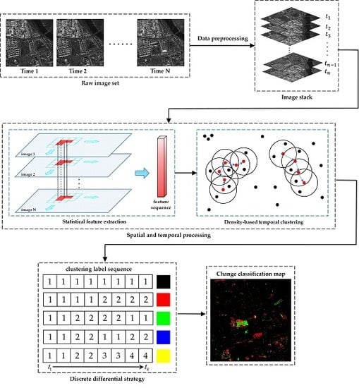
2.1. Time-Series SAR Data Preprocessing

Before running the time-series change detection algorithm, it is essential to perform several fundamental preprocessing operations on SAR images that contribute to reducing the impact of irrelevant factors (e.g., mismatched error and speckle noise) on change detection results. The preprocessing procedures involved in SAR image change detection are primarily radiometric calibration, co-registration, and speckle filtering. Radiometric calibration [29] minimizes the differences between the image radiometry and makes SAR images acquired on different dates comparable. The pixel values can represent the backscattering characteristics of ground objects after correction. Image co-registration is another important procedure for change detection that ensures that the spatial position of the same targets within different images is identical. Mis-registration will result in serious false alarms and generate many pseudo-change points in the detection results, thus the registration accuracy of multitemporal images must be at the sub-pixel level [30]. In addition, SAR images suffer inherent speckle noise due to the imaging mechanism, and speckle filtering is an indispensable step required to suppress the noise and improve the visual quality and interpretability of SAR images. For the time-series case, we employ the multitemporal despeckling method to reduce noise, in consideration of its remarkable effect on details and edge information preservation and its ability to conserve spatial resolution. In this paper, the GAMMA software packages [31] are used to implement radiometric calibration and co-registration, and we adopt multitemporal SAR block-matching and 3D filtering (MSAR_BM3D) [32] for denoising, which can greatly reduce the speckle effect and ensure the ground objects in filtering results are unchanged by searching similar points in spatiotemporal neighborhoods with non-local means.

2.2. Spatial Statistical Feature Extraction

SAR images are susceptible to speckle noise, which often affects the accuracy of applications that exploit SAR amplitude information, such as ground object classification and change detection. In particular, the fluctuation of original pixel value sequences caused by speckle noise may lead to a large amount of false alarms in time-series change detection results. The multitemporal filtering applied in the preprocessing stage has greatly suppressed speckle noise, but the traditional pixel-based methods may still be affected. Therefore, we extract features based on local statistics information to further reduce the influence of speckle noise before temporal clustering, which is the first function of this step.

In addition, image feature extraction is a key step in image recognition and classification tasks. In this work, it is necessary to simultaneously detect the changed region in space and classify the change pattern in time as accurately as possible, which requires that the selected features are not only able to represent the SAR image well, but also to distinguish between different change categories, and this is the main aim of this step. Prior knowledge plays an important role in the feature extraction process, considering that the areas in the experimental data are principally cities and buildings, we use the lognormal distribution to describe the statistical properties of SAR images [33] as it is a good representation of heterogeneous terrain in high resolution SAR data. The probability density function (PDF) of the lognormal distribution is as follows:

$$f\left(x\right)=\frac{1}{x\sigma \sqrt{2\pi }}exp\left(-\frac{{\left(lnx-\mu \right)}^2}{2{\sigma }^2}\right),$$

(1)

where $x$ is a positive random variable denoting the pixel amplitude in this study, $\mu$ and $\sigma$ denote the mean and standard deviation of $\ln x$, respectively.

We assume that the amplitudes of pixels in a local patch in SAR images follow a lognormal distribution with parameters $\left(\mu ,\sigma \right)$, i.e., $x_i~f_L\left(x;\mu ,\sigma \right),i=1,\dots w_0$, where $w_0$ is the total number of pixels in a patch. Specifically, each local patch is a square window centered at the $m$th pixel with size of $s\times s$ ($w_0=s\times s$), as shown in the feature extraction step in Figure 1. By sliding the window, the local regions corresponding to each center pixel can be obtained. Thus, the likelihood function for the parameters of a patch can be derived as follows:

$$L\left(\mu ,\sigma \left|x\right.\right)={\left(\frac{1}{\sigma \sqrt{2\pi }}\right)}^{w_0}\frac{1}{{{\displaystyle \prod }}_{i=1}^{w_0}{x}_i}exp\left(-\frac{1}{2{\sigma }^2}{{\displaystyle \sum }}_{i=1}^{w_0}{\left(\ln x_i-\mu \right)}^2\right),$$

(2)

The parameters are then obtained by Equation (3) according to the maximum likelihood estimation (MLE) method:

$$\widehat{\mu },\widehat{\sigma }=\underset{\mu ,\sigma }{argmax}L\left(\mu ,\sigma \left|x\right.\right),$$

(3)

By taking the partial derivative of the likelihood $L\left(·\right)$ with regard to the parameters $\left(\mu ,\sigma \right)$, respectively, and setting it to 0, we can derive the MLE of $\mu$ and $\sigma$:

$$\begin{gathered} \widehat{\mu }=\frac{1}{w_0}{\displaystyle \sum }_{i=1}^{w_0}ln{x}_i \\ {\widehat{\sigma }}^2=\frac{1}{w_0}{{\displaystyle \sum }}_{i=1}^{w_0}{\left(ln{x}_i-\mu \right)}^2. \end{gathered}$$

(4)

Here, the parameter $\widehat{\mu }$ is regarded as the statistical feature of each patch in SAR images, which is able to better suppress the speckle noise and represent the center scatterer of the patch because of the operation of the statistical mean and proper distribution selection.

2.3. Temporal Grouping Using a Density-Based Clustering Method

After extracting the statistical features of all images, an unsupervised method called density-based clustering of application with noise (DBSCAN) [34] is introduced to group the temporal feature sequence at every position. The DBSCAN method assumes that categories can be determined by the closeness of the sample distribution, thus a clustering category will be obtained by dividing closely connected samples into one class. Compared to traditional clustering methods, it does not need to specify the number of clusters in advance and can effectively process abnormal points and find clusters of arbitrary shapes, which is suitable for similar pixel grouping and change pattern identification in the temporal dimension.

Consider a set of temporal features $D=\left\{{\mu }_{l1},{\mu }_{l2},\dots ,{\mu }_{ln}\right\}$ at a certain position to be clustered, where $n$ is the number of SAR images, and $l$ denotes the same spatial location in the image. Let $\epsilon$ be the radius of the neighborhood in a sample and minPts be the minimum number of points required to form a dense region. The metric used in this study is the Euclidean distance. Some key concepts related to DBSCAN are defined as follows, and a diagram is given to better illustrate the relationships among these concepts (see Figure 2):

• Core point: for any sample ${\mu }_{lj}\in D$, it is regarded as a core point if at least minPts are included in the circle area centered on ${\mu }_{lj}$ with a radius of $\epsilon$.
• Directly density-reachable: ${\mu }_{li}$ is directly density-reachable from ${\mu }_{lj}$ if ${\mu }_{li}$ is within the distance $\epsilon$ of core point ${\mu }_{lj}$. Note that it does not satisfy the symmetry unless ${\mu }_{li}$ is also a core point.
• Density-reachable: ${\mu }_{li}$ is density-reachable from ${\mu }_{lj}$ if there is a sample sequence $p_1,p_2,\dots ,p_T$ with $p_1={\mu }_{li}, p_T={\mu }_{lj}$, and $p_{t+1}$ is directly density-reachable from $p_t$, where all samples in the sequence are the core points, or in other words, the density-reachable meets the transitivity.
• Outliers: ${\mu }_{lj}$ is an outlier or a noise point if it is not density-reachable from any other sample in $D$.

In Figure 2, we set the minPts to 4 as an example. The red points are core points because they all contain at least 4 points within the circle with radius of $\epsilon$. The green points are non-core points as they are directly-reachable from the adjacent red point and reachable from other red points, and these points form a single cluster. The blue point is an outlier and it is not reachable from any other point. On the basis of the above definitions, the clustering procedure can be summarized in Algorithm 1, as shown below.

Algorithm 1. Temporal clustering for the pixel sequence (DBSCAN).

Input: temporal features $D=\left\{{\mu }_{l1},{\mu }_{l2},\dots ,{\mu }_{ln}\right\}$ of the patch sequence and the neighborhood parameters $\left(\epsilon ,\mathrm{minPts}\right)$.

Output: the clustering labels for the pixel sequence.

1: Mark all samples in dataset $D$ as unvisited, initialize the cluster index $CI=0$;

2: for each sample $q$ in dataset $D$ do 3: if $q$ has been classified as a cluster or marked as noise then 4:   continue; 5: else 6:   if the samples contained in neighborhood of $q$ ($N_{\epsilon }\left(q\right)$) is less than minPts then 7:     Mark $q$ as a outlier or noise point; 8:   else 9:     Mark $q$ as a core point, create a new cluster $C$ and add all points in $N_{\epsilon }\left(q\right)$ to $C$, 10:     $CI=CI+1$ and assign the cluster index of $q$ as $CI$;

11:     for each point ($r$) unvisited in $N_{\epsilon }\left(q\right)$ do 12:       Add the point in $N_{\epsilon }\left(r\right)$ unclassified into any other cluster to $C$ if $N_{\epsilon }\left(r\right)$ contains at least minPts points; 13:       Assign the cluster index of $r$ as $CI$;

14:     end for 15:   end if 16: end if

17: end for

2.4. Classification with a Discrete Differential Strategy

In order to identify the temporal change pattern of each scatterer in space, the sequence of categories obtained after clustering should be classified. According to the clustering results, the change behavior in time can be divided into four types [26]: step change, impulse change, cycle change, and complex change (see

Table 1. The corresponding relation between different change types and category sequences.

Change Types	Number of Clusters	Category Sequence Example
Unchanged	1	{1,1,…}
Step change	2	{1,1,…,2,2,…}
Impulse change	2	{1,1,…,2,2,…,1,1,…}
Cycle change	2	{1,1,…,2,2,…,1,1,…,2,2,…}
Complex change	$\ge 3$	{1,1,…,2,2,…,3,3,…,4,4,…}

below). A step change means the ground object was unchanged at first but has changed since a certain date; its cluster label series form is {1,1,…,2,2,…}. An impulse change means the ground object was unchanged at the beginning, then changed since a certain date but has changed back to the original state since another date; its cluster label sequence form is {1,1,…,2,2,…,1,1,…}. A cycle change indicates that the ground feature changed periodically and the corresponding label sequence is {1,1,…,2,2,…,1,1,…,2,2,…}; the number of clusters of above change types is 2. Finally, changes with more than two clusters ($\ge 3$) are defined as complex changes because of the complicated transformation. For instance, newly-built shopping malls, residential areas, industrial zones, and other buildings are usually considered as step changes in the urban process, impulse changes and cycle changes correspond to the variation of construction facilities or moving targets such as cars, boats, and airplanes in high resolution images, and complex changes include the remaining cases of complicated change, e.g., changing from bare soil to agricultural land and then into buildings.

The clustering results are usually more complicated in practice and a fast classification method with generality is needed. Hence, we propose a strategy based on a first-order finite difference method to distinguish between different change patterns. The expression of the forward difference can be given by

$${\Delta }_{h}F\left(x\right)=F\left(x+h\right)-F\left(x\right),$$

(5)

where the spacing $h$ denotes the time interval between adjacent dates and is taken to be 1, and $F\left(x\right)$ is the cluster label of each pixel in time. After differential processing, the characteristics of each change type is prominent and easily distinguishable. For instance, the step change is reduced to an impulse response and the impulse change becomes two impulse responses with opposite positive and negative symbols.

2.5. Quantitative Evaluation Criteria

To verify the performance and effectiveness of each method, it is necessary to quantitatively evaluate the change detection results. Given the ground truth, a quantitative assessment can be obtained by comparing the detection results with a truth map. In bi-date change detection, a series of indicators based on the binary confusion matrix are often used. Analogously, we utilize multi-class confusion matrix-based indices that are extended from the binary case as the quantitative evaluation criteria for time-series change detection results. From the confusion matrix, the precision ($PR$) and recall ($RE$) of each change type are calculated and the comprehensive indices indicating overall performance are given by the macro F1-score ($F_{macro}$) and micro F1-score ($F_{micro}$) [35], which are defined as follows:

$$\begin{gathered} F_{macro}=\frac{1}{n}{\displaystyle \sum }_{i=1}^n{F}_i \\ {F}_i=\frac{2\times P{R}_i\times R{E}_i}{P{R}_i+R{E}_i} \\ P{R}_i=\frac{T{P}_i}{T{P}_i+F{P}_i} \\ R{E}_i=\frac{T{P}_i}{T{P}_i+F{N}_i}, \end{gathered}$$

(6)

$$\begin{gathered} F_{micro}=\frac{2\times P{R}_{micro}\times R{E}_{micro}}{P{R}_{micro}+R{E}_{micro}}=\frac{{{\displaystyle \sum }}_{i=1}^{n}T{P}_i}{N} \\ P{R}_{micro}=\frac{{{\displaystyle \sum }}_{i=1}^{n}T{P}_i}{{{\displaystyle \sum }}_{i=1}^{n}T{P}_i+{{\displaystyle \sum }}_{i=1}^{n}F{P}_i} \\ R{E}_{micro}=\frac{{{\displaystyle \sum }}_{i=1}^{n}T{P}_i}{{{\displaystyle \sum }}_{i=1}^{n}T{P}_i+{{\displaystyle \sum }}_{i=1}^{n}F{N}_i}, \end{gathered}$$

(7)

where $T{P}_i$ denotes the number of pixels correctly classified as change type $i$, $F{P}_i$ denotes the number of pixels incorrectly classified as type $i$, $F{N}_i$ denotes the number of pixels of type $i$ that are incorrectly classified as other types, and $F_i$ denotes the F1-score of each class. $N$ is the total pixel number of the image, $i=1,\dots ,n$, and $n$ is the number of change types (here n = 5).

The macro-averaging and micro-averaging measure the accuracy of multi-class classification tasks from different angles. Macro-averaging gives each class the same weight, while micro-averaging gives the same weight to each sample. In other words, the former considers each class separately and the latter takes all categories into account simultaneously. In addition, the micro-averaging is actually equivalent to the overall accuracy ($OA$) according to Equation (7).

3. Experiments and Results

3.1. Study Site and Dataset Description

The proposed approach is tested on a time-series dataset of TerraSAR-X remote sensing images. TerraSAR-X is a commercial Earth observation SAR satellite working at X-band that was jointly developed by the German government and industrial circles and was launched in 2007. It can acquire high-quality SAR images of all areas with a 1~16m spatial resolution under different imaging modes, and the revisit period is shortened to 11 days. The high resolution of TerraSAR-X images enables the accurate mapping of independent buildings, urban structures, and infrastructure, which are commonly used in change detection tasks with regard to the evolution of cities. The study site in this work is located in the Tongzhou District of Beijing, China (shown in Figure 3a, with the district line in red). As the administrative sub-center of the capital, Tongzhou has been undergoing rapid changes in recent years, and the demolition and construction of buildings in this area is conducive to validating the effectiveness of different change detection algorithms. Figure 3b shows the first image of the multitemporal dataset, which consists of 8 SAR images of the same region acquired from January 22, 2012 to May 20, 2013 with a size of 1000$\times$1000 pixels and 3 m resolution. The pixel spacing in range and azimuth directions are 0.9 m and 1.9 m, respectively. The ground features covered by the dataset are mainly residential areas, roads, bridges, and a river, and the dominating change is caused by building constructions.

3.2. Experimental Setup and Paramter Setting

In this paper, two experiments were designed to verify the performance of the proposed method based on a time-series dataset: a synthetic simulation experiment and a realistic data experiment. The change region and change type can be set manually in the synthetic test, which ensures the accuracy of the ground truth and compares each method under a relatively ideal condition. Then, the proposed approach was evaluated in the real case to demonstrate the effectiveness for time-series change detection. Both experiments were comprehensively analyzed in terms of qualitative results and quantitative indices.

In the two experiments, our method was compared with the other three multitemporal change detection methods to demonstrate its superiority, namely, normalized cut on change criterion matrix (NORCAMA) [26] and two improved approaches using local information according to the NORCAMA framework called the normalized cut on Kullback–Leibler divergence-based change matrix (NOR_KLD) [25] and the normalized cut on two-sample Kolmogorov-Smirnov test-based change matrix (NOR_KS2) [36], respectively. The optimal parameters of all experiments were obtained by the trial-and-error method. The parameters involved in the proposed framework are size of local window in spatial feature extraction and the $\epsilon$ and minPts in temporal clustering. These were set based on the heuristic method of the k-distance graph [34,37,38]: the window size was 3$\times$3, $\epsilon =0.3~0.4$, and $\mathrm{minPts}=2$. The details of the parameters set for the three comparison methods are the following: (1) in the NORCAMA approach, the threshold was set by ${\tau }^{GLRT}= 0.9$ with a false alarm rate of 1%; (2) the local window size of NOR_KLD was 5$\times$5; (3) in NOR_KS2, the significant level was set as ${\alpha }_{KS2} = 0.05$, and the window size was 7$\times$7.

It should be noted that the spatial window sizes adopted by the three local statistics-based approaches of the proposed method, NOR_KLD, and NOR_KS2 are different because they are the optimal sizes obtained by the trial-and-error method, which ensures that the selected parameters reflect the best performance of each approach. Therefore, the window sizes used in different methods may not be the same. To make the process of size selection more clear, the influence of different window sizes on the quantitative results (macro F1-score and micro F1-score) of synthetic time-series datasets (see Section 3.3.1) for the above three approaches are analyzed and shown in Figure 4. It can be seen from the figure that the highest accuracy of the proposed method, NOR_KLD, and NOR_KS2 is achieved when the window sizes are 3$\times$3, 5$\times$5, and 7$\times$7, respectively. Accordingly, these are chosen as the optimal sizes of the local window in each method.

3.3. Experimental Results and Analysis

3.3.1. Test on Synthetic Time-Series SAR Images

As shown in Figure 5, the simulated experiment is designed on the basis of real SAR images. Firstly, 8 co-registered TerraSAR-X images are used as input for multitemporal filtering, and one denoised image is approximately taken as the noise-free image (see Figure 5a). Then, the noise-free image is regarded as a base map where the change is added at different times. The change areas added therein are 10 small rectangles that are randomly distributed in images with a length and width of 15~25 pixels, including all 4 change types: step change (in red), impulse change (in green), cycle change (in blue), and complex change (in yellow). The details of the sizes of the 10 change areas are listed in

Table 2. The size of 10 change areas.

Change Areas	Step Change (Red)			Cycle Change (Blue)			Impulse Change (Green)		Complex Change (Yellow)
Length	20	23	16	19	17	17	18	19	20	21
Width	20	23	18	25	16	23	20	22	17	18

. Finally, 1-Look speckle noise is added in all images to generate 6 realistic SAR synthetic images. Figure 5c shows an example of each change type. The ground truth map is shown in Figure 5b.

The time-series change detection and classification results of the synthetic SAR images are given in Figure 6. The spatial change detection results are first analyzed, and it can be seen from the figure that the 10 rectangular change regions have been well detected by the four methods. However, there are many false alarm pixels in the detection map of NORCAMA (shown in Figure 6a) due to speckle noise, which is difficult to avoid in a pixel-based approach. In contrast, the other three methods take advantage of local statistical information to effectively reduce noise and the false positive rate, thus the detection accuracy of the unchanged regions (in black) shown in Figure 6b–d has been greatly improved. The temporal classification performance of each method for the detected change regions is then compared. All four methods show good classification results for step changes, impulse changes, and cycle changes, while a relatively large difference occurs when classifying complex change. To compare different methods more clearly, a white rectangle is used to point out the area where the complex changes take place, as shown in Figure 7. It can be observed that the proposed method shows better classification performance on the yellow block in the lower left corner, especially in the preservation of edge smoothness. In addition, our method shows the least misclassification of the type of complex change. This may be due to the robustness of DBSCAN to noise. On the whole, the proposed method achieves the best detection and classification results on synthetic SAR data from the aspect of qualitative analysis.

To assess the change detection and classification results among different approaches more precisely, we adopt indices of macro F1-score and micro F1-score based on a multi-class confusion matrix, as previously mentioned. The quantitative results obtained by the four methods are shown in Table 3 and

Table 4. Quantitative comparison of change classification accuracy for different methods using synthetic data.

Indices (%)	NORCAMA	KLD	KS2	Proposed
Unchanged
precision	99.99	99.98	99.99	99.99
recall	99.26	99.86	99.88	99.95
F1-score	99.63	99.92	99.94	99.97
Step change
precision	34.16	63.59	69.96	81.50
recall	99.75	96.88	97.04	99.92
F1-score	50.89	76.78	81.31	89.77
Impulse change
precision	16.50	60.94	58.56	82.67
recall	95.37	74.81	98.46	98.07
F1-score	28.13	67.17	73.44	89.71
Cycle change
precision	47.83	68.86	80.51	84.90
recall	99.56	98.51	99.12	99.82
F1-score	64.61	81.06	88.85	91.76
Complex change
precision	74..36	62.73	93.77	100.00
recall	80.78	57.66	83.84	86.21
F1-score	77.44	60.09	88.53	92.60
Macro F1-score	64.14	77.00	86.41	92.76
Micro F1-score	99.24	99.80	99.86	99.93

. Table 3 lists the confusion matrix for each method in detail, which calculates statistics of the classified pixel number by comparing the actual label in the ground truth with the predicted types and represents whether the algorithm is confusing different classes. In Table 4, the precision, recall, and F1-score of five classes are calculated according to the confusion matrix, which embodies the classification accuracy of each approach in different change types. From the table, we can see that the highest macro F1-score and micro F1-score are both achieved by the proposed method. Our method also attained the best results in the classification of every single category. For the index of micro F1-score (namely overall accuracy), the gap among all approaches is small as the unchanged class accounts for a large proportion of all types, i.e., data is imbalanced. This is common in change detection applications because the changed ground objects are few compared to the unchanged regions. Therefore, macro-averaging is introduced to provide a more comprehensive evaluation of each method, especially in terms of classification capability. As a whole, the quantitative results show good agreement with the above qualitative analysis.

3.3.2. Test on Realistic Time-Series SAR Images

A synthetic experiment is, after all, a relatively ideal circumstance, thus it can achieve excellent detection and classification effects. Nevertheless, changes occurring in real ground features will be more complex than the synthetic case, and a dataset based on multitemporal TerraSAR-X data is accordingly created to further verify the effectiveness of the proposed algorithm Figure 8 presents the time-series change detection results of all methods on this dataset. The ground truth map is labeled manually and shown in Figure 8a. Figure 8b is the change detection result using the NORCAMA method. Although it shows a good performance on the classification of temporal change patterns, the result is inevitably affected by serious speckle noise, even with pre-filtering, because of the pixel-based operation. Figure 8c,d give the results of NOR_KLD and NOR_KS2, respectively. As can be seen from the figures, these two methods have a larger number of false alarm pixels than NORCAMA. The main reason may be the generation process of the similarity matrix, which will influence the clustering result. In the previous synthetic experiment, the results obtained show a good effect because the pixel amplitude changes little in time, whereas in practice, neither method handles complicated changes with large fluctuations well. The result of the proposed method is shown in Figure 8e, where speckle noise is further suppressed due to the exploitation of local statistical information. Additionally, the change classification accuracy is enhanced greatly by combining the extracted features and a density-based clustering approach. Thus, overall, our method achieves the best qualitative result compared with the other three methods.

The multi-class confusion matrices for the four methods are shown in Table 5. The changed regions consist mainly of step changes and impulse changes since the study area was undergoing the demolition and construction of buildings during the acquisition time due to the establishment of the sub-center plan. In contrast, the detected cycle changes and complex changes are few. In order to analyze and reveal the details of changes in buildings over a long period of time, we chose a representative region as a sample, as shown in Figure 9. Figure 9a is the change detection and classification result of the selected area, which mainly consists of step changes (in red) and impulse changes (in green). Figure 9b illustrates the detailed change process of the building within the region in time, and the corresponding optical images recording key changes acquired on March 4, 2013 and September 26, 2013 are given in Figure 9c. It can be seen from these figures that the red step changes on both sides were caused by the completion of two rows of residential buildings, and the green impulse change in the middle is due to the dismantlement of the construction facilities after finishing the buildings. The time-series SAR dataset records the evolution of the city from the construction process of a building to the urbanization of an entire region, which is of great significance to urban management.

The precision, recall, and F1-score of each change type are listed below in

Table 6. Quantitative comparison of change classification accuracy for different methods in the realistic case.

Indices (%)	NORCAMA	KLD	KS2	Proposed
Unchanged
precision	99.35	98.80	99.32	99.64
recall	98.17	96.21	94.84	98.85
F1-score	98.76	97.49	97.03	99.24
Step change
precision	65.35	47.00	40.47	77.86
recall	81.18	62.24	69.39	88.23
F1-score	72.41	53.56	51.13	82.72
Impulse change
precision	51.55	22.94	23.21	63.87
recall	75.32	51.51	66.41	90.19
F1-score	61.21	31.74	34.39	74.78
Cycle change
precision	27.94	7.56	8.13	50.95
recall	62.28	41.58	44.87	75.35
F1-score	38.58	12.79	13.77	60.80
Complex change
precision	55.37	19.26	15.60	70.05
recall	56.90	30.63	64.69	71.05
F1-score	56.13	23.65	25.14	70.54
Macro F1-score	65.41	43.85	44.29	77.62
Micro F1-score	97.46	94.85	93.88	98.46

. Compared to the synthetic result, the macro and micro F1-score obtained by NORCAMA shows a relatively stable performance in the realistic situation because of the likelihood ratio change matrix. However, the quantitative indices derived from NOR_KLD and NOR_KS decrease significantly, which indicates that the generation methods for the similarity matrices adopted in the two approaches are not competent with real images. Figure 10 clearly compares the classification accuracy of five change patterns and the comprehensive performance of each method based on F1-scores. It can be seen that the micro F1-score, namely overall accuracy, is close to the unchanged F1-score, this can be explained by the fact that the unchanged pixels occupy most of the area in the image. Meanwhile, NORCAMA and our method yield better a classification results for four types of change due to their robustness. To sum up, the proposed method still shows the best results for both single pattern classification accuracy and overall effect, which is consistent with the above qualitative analysis.

Considering that every pixel series needs temporal clustering, computational efficiency is another important indicator. Therefore, we undertake a comparison and analysis of the runtime for each algorithm.

Table 7. Computational time (in seconds) for time-series change detection of 1000 × 1000 × 8 SAR images.

Efficiency	NORCAMA	NOR_KLD	NOR_KS2	Proposed
runtime	582 s	776 s	923 s	48 s

presents the computational time for each method running on a computer with an Intel i7 CPU at 2.80 GHz (4 cores) and 8GB RAM. All algorithms are implemented in the MATLAB language and speeded up using parallel operation. The runtimes of NORCAMA, NOR_KLD, and NOR_KS2 are composed of two parts: similarity matrix generation and spectral clustering, with the latter step being very time-consuming because of the high time complexity. It can be seen from the table that the proposed framework achieves the fastest runtime and is significantly faster than the other three methods.

4. Discussion

With the development of satellite remote sensing technology, the spatial and temporal resolution of SAR images are both getting higher and higher. Time-series change detection of high resolution SAR images is becoming an important approach to reveal the spatiotemporal changes of ground objects and mine out interesting information. Compared with other multitemporal change detection approaches, the method proposed in this paper can remarkably improve change detection and classification accuracy, mainly owing to two factors: (1) local information is exploited by extracting the statistical features of each patch according to the appropriate distribution of ground objects; (2) temporal grouping using a density-based clustering method called DBSCAN can improve classification accuracy without a pre-determined cluster number and considerably reduce the runtime. In both synthetic and realistic experiments, our method achieves more satisfactory results than the other three methods tested.

By adopting the discrete differential strategy, we are easily able to identify different change patterns and obtain the final classification results. In addition, more temporal change information can be uncovered based on the differential results, which are shown in Figure 11. For time-series change detection, the ground objects may change many times over a long period of time, thus knowing when they first and last changed will contribute to urban planning and management. Figure 11a,b show when the first and last detected change occurred, respectively, during January 22, 2012 to May 20, 2013, where 0 (black) means no change over the whole time span, 1 means first or last change occurred between $t_1$ and $t_2$, 2 means first or last change occurred between $t_2$ and $t_3$, etc. For example, the building within white box area shown in Figure 11d only changed once over the timespan, so its first detected change is the same as the last detected change, both of which occurred between $t_7$ and $t_8$. Figure 11c shows the frequency of changes within the acquisition time range. It can be observed from the figure that most objects have only changed once or twice, which indicates that the study site is relatively stable and that changes occur infrequently.

Through the abovementioned multidimensional change information, the time-series change detection approach can not only provide reliable information for urban planning and supervision, but it can also serve as an important basis for ecological environment monitoring and protection, which has a wide prospect in real-world applications.

5. Conclusions

To improve change detection and classification accuracy and reduce the influence of speckle noise for multitemporal SAR images, a novel and highly efficient time-series change detection method that takes advantage of local information and temporal similarity was proposed in this paper. Our method mainly includes three steps. Firstly, the spatial statistical features of each local patch in SAR images at any date were extracted based on MLE to suppress speckle noise and make the next classification of change patterns more accurate. Then, because of its outstanding performance, we utilized the density-based clustering method called DBSCAN to implement temporal grouping. Finally, a discrete differential strategy was adopted to process the clustering results and identify the change patterns over time. To validate the effectiveness of the proposed method, we carried out two experiments based on a synthetic and realistic case using a time-series SAR dataset acquired by TerraSAR-X in the Tongzhou District of Beijing, China, which is undergoing tremendous changes. The outcome showed that our method achieved the best performance in both tests in terms of both the qualitative and quantitative results. In addition, we discussed the differential results and found that more temporal information can be obtained, including the change frequency and when changes happened. In future research, we will consider further improving the classification accuracy and reducing speckle noise, especially in realistic time-series SAR images.

References

1. Malila, W.A. Change vector analysis: An approach for detecting forest changes with Landsat. In Proceedings of the LARS symposia, West Lafayette, IN, USA, 3–6 June 1980; p. 385. [Google Scholar]
2. Singh, A. Review article digital change detection techniques using remotely-sensed data. Int. J. Remote Sens. 1989, 10, 989–1003. [Google Scholar] [CrossRef]
3. Lu, D.; Mausel, P.; Brondizio, E.; Moran, E. Change detection techniques. Int. J. Remote Sens. 2004, 25, 2365–2401. [Google Scholar] [CrossRef]
4. El-Kawy, O.A.; Rød, J.; Ismail, H.; Suliman, A. Land use and land cover change detection in the western Nile delta of Egypt using remote sensing data. Appl. Geogr. 2011, 31, 483–494. [Google Scholar] [CrossRef]
5. Chen, X.; Chen, J.; Shi, Y.; Yamaguchi, Y. An automated approach for updating land cover maps based on integrated change detection and classification methods. ISPRS J. Photogramm. Remote Sens. 2012, 71, 86–95. [Google Scholar] [CrossRef]
6. Gamba, P.; Dell’Acqua, F.; Lisini, G. Change detection of multitemporal SAR data in urban areas combining feature-based and pixel-based techniques. IEEE Trans. Geosci. Remote Sens. 2006, 44, 2820–2827. [Google Scholar] [CrossRef]
7. Ban, Y.; Yousif, O.A. Multitemporal spaceborne SAR data for urban change detection in China. IEEE J. Sel. Top. Appl. Earth Obs. Remote Sens. 2012, 5, 1087–1094. [Google Scholar] [CrossRef]
8. Stramondo, S.; Bignami, C.; Chini, M.; Pierdicca, N.; Tertulliani, A. Satellite radar and optical remote sensing for earthquake damage detection: Results from different case studies. Int. J. Remote Sens. 2006, 27, 4433–4447. [Google Scholar] [CrossRef]
9. Tewkesbury, A.P.; Comber, A.J.; Tate, N.J.; Lamb, A.; Fisher, P.F. A critical synthesis of remotely sensed optical image change detection techniques. Remote Sens. Environ. 2015, 160, 1–14. [Google Scholar] [CrossRef] [Green Version]
10. Bazi, Y.; Bruzzone, L.; Melgani, F. An unsupervised approach based on the generalized Gaussian model to automatic change detection in multitemporal SAR images. IEEE Trans. Geosci. Remote Sens. 2005, 43, 874–887. [Google Scholar] [CrossRef] [Green Version]
11. Moser, G.; Serpico, S.B. Generalized minimum-error thresholding for unsupervised change detection from SAR amplitude imagery. IEEE Trans. Geosci. Remote Sens. 2006, 44, 2972–2982. [Google Scholar] [CrossRef] [Green Version]
12. Gong, M.; Zhou, Z.; Ma, J. Change detection in synthetic aperture radar images based on image fusion and fuzzy clustering. IEEE Trans. Image Process. 2012, 21, 2141–2151. [Google Scholar] [CrossRef] [PubMed]
13. Gong, M.; Zhao, J.; Liu, J.; Miao, Q.; Jiao, L. Change detection in synthetic aperture radar images based on deep neural networks. IEEE Trans. Neural Netw. Learn. Syst. 2016, 27, 125–138. [Google Scholar] [CrossRef]
14. Breit, H.; Fritz, T.; Balss, U.; Lachaise, M.; Niedermeier, A.; Vonavka, M. TerraSAR-X SAR processing and products. IEEE Trans. Geosci. Remote Sens. 2010, 48, 727–740. [Google Scholar] [CrossRef]
15. Torres, R.; Snoeij, P.; Geudtner, D.; Bibby, D.; Davidson, M.; Attema, E.; Potin, P.; Rommen, B.; Floury, N.; Brown, M. GMES Sentinel-1 mission. Remote Sens. Environ. 2012, 120, 9–24. [Google Scholar] [CrossRef]
16. Sun, J.; Yu, W.; Deng, Y. The SAR payload design and performance for the GF-3 mission. Sensors 2017, 17, 2419. [Google Scholar] [CrossRef]
17. Coppin, P.; Lambin, E.; Jonckheere, I.; Muys, B. Digital change detection methods in natural ecosystem monitoring: A review. In Analysis of Multi-Temporal Remote Sensing Images; World Scientific: Singapore, 2002; pp. 3–36. [Google Scholar]
18. Radke, R.J.; Andra, S.; Al-Kofahi, O.; Roysam, B. Image change detection algorithms: A systematic survey. IEEE Trans. Image Process. 2005, 14, 294–307. [Google Scholar] [CrossRef]
19. Bruzzone, L.; Prieto, D.F. Automatic analysis of the difference image for unsupervised change detection. IEEE Trans. Geosci. Remote Sens. 2000, 38, 1171–1182. [Google Scholar] [CrossRef]
20. Conradsen, K.; Nielsen, A.A.; Skriver, H. Determining the points of change in time series of polarimetric SAR data. IEEE Trans. Geosci. Remote Sens. 2016, 54, 3007–3024. [Google Scholar] [CrossRef]
21. Dogan, O.; Perissin, D. Detection of Multitransition Abrupt Changes in Multitemporal SAR Images. IEEE J. Sel. Top. Appl. Earth Obs. Remote Sens. 2014, 7, 3239–3247. [Google Scholar] [CrossRef]
22. Muro, J.; Canty, M.; Conradsen, K.; Hüttich, C.; Nielsen, A.A.; Skriver, H.; Remy, F.; Strauch, A.; Thonfeld, F.; Menz, G. Short-Term Change Detection in Wetlands Using Sentinel-1 Time Series. Remote Sens. 2016, 8, 795. [Google Scholar] [CrossRef]
23. Liu, W.; Yang, J.; Zhao, J.; Shi, H.; Yang, L. An unsupervised change detection method using time-series of PolSAR images from radarsat-2 and gaofen-3. Sensors 2018, 18, 559. [Google Scholar]
24. Atto, A.M.; Trouvé, E.; Berthoumieu, Y.; Mercier, G. Multidate divergence matrices for the analysis of SAR image time series. IEEE Trans. Geosci. Remote Sens. 2013, 51, 1922–1938. [Google Scholar] [CrossRef]
25. Le, T.T.; Atto, A.M.; Trouve, E. Change analysis using multitemporal Sentinel-1 SAR images. In Proceedings of the Geoscience & Remote Sensing Symposium, Milan, Italy, 26–31 July 2015. [Google Scholar]
26. Su, X.; Deledalle, C.-A.; Tupin, F.; Sun, H. NORCAMA: Change analysis in SAR time series by likelihood ratio change matrix clustering. ISPRS J. Photogramm. Remote Sens. 2015, 101, 247–261. [Google Scholar] [CrossRef] [Green Version]
27. Bujor, F.; Trouvé, E.; Valet, L.; Nicolas, J.M.; Rudant, J.P. Application of log-cumulants to the detection of spatiotemporal discontinuities in multitemporal SAR images. Geosci. Remote Sens. IEEE Trans. 2004, 42, 2073–2084. [Google Scholar] [CrossRef]
28. Quin, G.; Pinel-Puyssegur, B.; Nicolas, J.-M.; Loreaux, P. MIMOSA: An automatic change detection method for SAR time series. IEEE Trans. Geosci. Remote Sens. 2014, 52, 5349–5363. [Google Scholar] [CrossRef]
29. Freeman, A. SAR calibration: An overview. IEEE Trans. Geosci. Remote Sens. 1992, 30, 1107–1121. [Google Scholar] [CrossRef]
30. Townshend, J.R.; Justice, C.O.; Gurney, C.; McManus, J. The impact of misregistration on change detection. IEEE Trans. Geosci. Remote Sens. 1992, 30, 1054–1060. [Google Scholar] [CrossRef] [Green Version]
31. Werner, C.; Wegmüller, U.; Strozzi, T.; Wiesmann, A. Gamma SAR and interferometric processing software. In Proceedings of the Ers-Envisat Symposium, Gothenburg, Sweden, 16–20 October 2000; p. 1620. [Google Scholar]
32. Chierchia, G.; Gheche, M.E.; Scarpa, G.; Verdoliva, L. Multitemporal SAR Image Despeckling Based on Block-Matching and Collaborative Filtering. IEEE Trans. Geosci. Remote Sens. 2017, 55, 5467–5480. [Google Scholar] [CrossRef]
33. Lv, X.; Yazıcı, B.; Zeghal, M.; Bennett, V.; Abdoun, T. Joint-Scatterer Processing for Time-Series InSAR. IEEE Trans. Geosci. Remote Sens. 2014, 52, 7205–7221. [Google Scholar]
34. Ester, M.; Kriegel, H.-P.; Sander, J.; Xu, X. A density-based algorithm for discovering clusters in large spatial databases with noise. In Proceedings of the Kdd, Portland, OR, USA, 2–4 August 1996; pp. 226–231. [Google Scholar]
35. Yang, Y. An evaluation of statistical approaches to text categorization. Inf. Retr. 1999, 1, 69–90. [Google Scholar] [CrossRef]
36. Yuan, J.; Lv, X.; Li, R. A Speckle Filtering Method Based on Hypothesis Testing for Time-Series SAR Images. Remote Sens. 2018, 10, 1383. [Google Scholar] [CrossRef]
37. Sander, J.; Ester, M.; Kriegel, H.-P.; Xu, X. Density-based clustering in spatial databases: The algorithm gdbscan and its applications. Data Min. Knowl. Discov. 1998, 2, 169–194. [Google Scholar] [CrossRef]
38. Schubert, E.; Sander, J.; Ester, M.; Kriegel, H.P.; Xu, X. DBSCAN revisited, revisited: Why and how you should (still) use DBSCAN. ACM Trans. Database Syst. (Tods) 2017, 42, 19. [Google Scholar] [CrossRef]
Figure 1. The workflow of the proposed time-series change detection method.
Remotesensing 11 00926 g001
Figure 2. The relationships among key concepts of density-based clustering of application with noise (DBSCAN) (minPts = 4 is used as an example).
Remotesensing 11 00926 g002
Figure 3. The time-series dataset of TerraSAR-X remote sensing images in the Tongzhou District of Beijing: (a) The study site; (b) The first scene of the dataset and corresponding optical image.
Remotesensing 11 00926 g003
Figure 4. Quantitative results of macro F1-score and micro F1-score for three local statistics-based approaches with different spatial window sizes (other parameters are fixed): (a) The proposed method; (b) normalized cut on Kullback–Leibler divergence-based change matrix (NOR_KLD); (c) normalized cut on two-sample Kolmogorov-Smirnov test-based change matrix (NOR_KS2).
Remotesensing 11 00926 g004
Figure 5. The synthetic time-series synthetic aperture radar (SAR) dataset (6 1-Look images): (a) The base map of an approximately noise-free image; (b) Ground truth of manually set changes; (c) Example of four change patterns (black: no change, red: step change, green: impulse change, blue: cycle change and yellow: complex change).
Remotesensing 11 00926 g005
Figure 6. The time-series change detection and classification results of synthetic case: (a) normalized cut on change criterion matrix (NORCAMA); (b) NOR_KLD; (c) NOR_KS2; (d) Proposed method.
Remotesensing 11 00926 g006
Figure 7. Classification results for complex changes in the white box area: (a) NORCAMA; (b) NOR_KLD; (c) NOR_KS2; (d) Proposed method.
Remotesensing 11 00926 g007
Figure 8. The time-series change detection and classification results using realistic data: (a) Ground truth map; (b) NORCAMA; (c) NOR_KLD; (d) NOR_KS2; (e) Proposed method.
Remotesensing 11 00926 g008
Figure 9. Change detection result of a representative sample in the realistic case: (a) The cropped change classification result; (b) The details of the change process across time within the cropped area; (c) Corresponding optical images (2013.03.04 and 2013.09.26) of the area.
Remotesensing 11 00926 g009
Figure 10. Quantitative comparison of change classification accuracies (F1-score) for different methods.
Remotesensing 11 00926 g010
Figure 11. Multidimensional temporal change maps: (a) map when the first detected changes happened; (b) map when the last detected changes happened; (c) change frequency map (number of changes); (d) change process of buildings in the white box area over time.
Remotesensing 11 00926 g011