Article

Analysis of Ku- and Ka-Band Sea Surface Backscattering Characteristics at Low-Incidence Angles Based on the GPM Dual-Frequency Precipitation Radar Measurements

1
First Institute of Oceanography, Ministry of Natural Resources, Qingdao 266061, China
2
Oceanic telemetry Engineering and Technology Research Center, Ministry of Natural Resources, Qingdao 266061, China
3
School of Earth Science and Technology, China University of Petroleum, Qingdao 266580, China
*
Author to whom correspondence should be addressed.
Remote Sens. 2019, 11(7), 754; https://doi.org/10.3390/rs11070754
Submission received: 30 January 2019 / Revised: 26 March 2019 / Accepted: 26 March 2019 / Published: 28 March 2019
(This article belongs to the Special Issue Radar Remote Sensing of Oceans and Coastal Areas)

Abstract

:
The co-located normalized radar backscatter cross section measurements from the Global Precipitation Measurement (GPM) Ku/Ka-band dual-frequency precipitation radar (DPR) and sea surface wind; wave and temperature observations from the National Data Buoy Center (NDBC) moored buoys are used to analyze the dependence and sensitivity of Ku- and Ka-band backscatter on surface conditions at low-incidence angles. Then the potential for inverting wind and wave parameters directly from low-incidence σ0 measurements is discussed. The results show that the KaPR σ0 is more sensitive to surface conditions than the KuPR σ0 overall. Nevertheless; both the KuPR σ0 and KaPR σ0 are strongly correlated with wind speed (U10) and average wave steepness (δa) with the exception of specific transitional incidence angles. Moreover, U10 and δa could be retrieved from pointwise σ0 near nadir and near 18°. Near 18°; wind direction information is needed as the effect of wind direction on σ0 becomes increasingly significant with incidence angle. To improve the performance of U10 retrieval; especially for low U10; auxiliary δa information would be most helpful; and sea surface temperature is better taken into account. Other wave parameters; such as significant wave height; wave period and wave age; are partly correlated with σ0. It is generally more difficult to retrieve those parameters directly from pointwise σ0. For the retrieval of those wave parameters; various auxiliary information is needed. Wind direction and wave direction cannot be retrieved from pointwise σ0.

Graphical Abstract

1. Introduction

Spaceborne observations of the ocean surface with active microwave instruments have been performed routinely for more than four decades since the launch of SeaSat in 1978, with most of the sensors working at moderate incidence angles (i.e., 16 ° θ 65 ° ) and near-vertical incidence angles (i.e., θ 1 ° ). However, in recent years, an increasing number of spaceborne radar systems, including the Ku-band precipitation radar on the Tropical Rainfall Mapping Mission (TRMM PR), the Ku/Ka-band dual-frequency precipitation radar on the Global Precipitation Measurement mission (GPM DPR), the Ku-band surface wave investigation and monitoring radar on the China–France Oceanography SATellite (CFOSAT SWIM) and the Ka-band radar interferometer on the Surface Water Ocean Topography mission (SWOT KaRin), measure the ocean surface at low-incidence angles as such measurements have great potential to obtain the information on sea surface winds and waves very easily based on the simple quasi-specular reflection theory (e.g., [1,2,3,4]). This triggers the need for well understanding of the characteristics of radar backscatter at Ku- and Ka-band at low-incidence angles.
For low-incidence angles, a few studies (e.g., [1,5,6,7]) have been devoted to investigating the effects of ocean wind and wave characteristics on the normalized radar backscatter cross section σ0 at Ku-band. For example, Freilich and Vanhoff [1] constructed fully empirical tabular functions relating σ0 to wind speed for incidence angles from 0° to 18° using the co-located cross-section measurements from TRMM PR and wind speed estimates from TRMM Microwave Imager (TMI). Tran et al. [5] documented the relationships between σ0, wind speed and significant wave height based on the collocations between the σ0 measurements from TRMM PR, the wind speed data from the European Centre for Medium-Range Weather Forecast (ECMWF) and the significant wave height observations from the Jason-1 and ENVISAT altimeters. Chu et al. [6] investigated the effects of wind direction on σ0 at low-incidence angles by analyzing the upwind/downwind asymmetry and upwind/crosswind anisotropy based on the collocations between PR measurements and buoy observations. Chu et al. [7] analyzed the relationships between σ0 and integrated wind and wave parameters (e.g., wind speed, wind direction, significant wave height, wave period, wave steepness, and wave age) at low-incidence angles for different sea states based on the co-located PR/buoy data. In general, the characteristics of σ0 at Ku-band are well understood and widely published. However, for the σ0 at Ka-band, only individual studies investigated its dependence on wind speed and wind direction based on the airborne and wind-wave tank observations [8,9,10]. These analyses are still not deep enough as the observation data concerning σ0 at Ka-band are relatively scarce, and the speciality needs further research.
As a successor of TRMM satellite, GPM is a mission that covers the low-incidence angle range with a dual-frequency precipitation radar system composed of two precipitation radars (PRs), the KuPR on the Ku-band with ±18° scan angle and the KaPR on the Ka-band with ±9° scan angle. Here, the GPM KuPR and KaPR measurements are used to further analyze the effects of surface wind, wave and other relevant environmental parameters on radar backscatter at Ku- and Ka-band, and consequently to better understand the possibilities for inversion of those parameters directly from the σ0 measurements at low-incidence angles. This paper is organized as follows. Section 2 describes the data sets and methods for collecting matchups. In Section 3, the dependence and sensitivity of the Ku- and Ka-band σ0 on different surface dynamic environmental parameters are systematically compared and analyzed. Section 4 discusses the possibilities for inversion of wind and wave parameters from low-incidence observations. A summary and the main conclusions are given in Section 5.

2. Materials and Methods

2.1. Global Precipitation Measurement Dual-Frequency Precipitation Radar (GPM DPR) Data

GPM is an international satellite mission to measure global precipitation, which is similar to but more expanded than TRMM. The GPM satellite, launched on February 27th, 2014, carries the first spaceborne Ku/Ka-band dual-frequency precipitation radar (DPR) providing new and unexplored data for not only the tropical zone but also mid- to high-latitude areas at a 65° inclined non-sun-synchronous orbit. In particular, the KaPR operates at 35.5 GHz with a nadir oriented antenna that scans a 125-km ground swath providing a 5 km × 5 km surface footprint over angular range between −9° and 9°. The KuPR operates at 13.6 GHz and sweeps a wider 245-km swath but with the same 5 km × 5 km resolution over angular range between −18° and 18°. The KuPR and KaPR acquire data nearly simultaneously within the inner 125-km swath. The KuPR acquires data in the outer portion of the full 245-km swath, while the KaPR operates in the high-sensitivity mode to measure the interlaced fields [11].
The data product used herein is the GPM DPR Level 2 standard product (ver. 5) obtained from the Globe Portal System (G-Portal) of the Japanese Aerospace Exploration Agency (JAXA). The product consists of three types of data, namely the Normal Swath (NS) of the KuPR, the co-localized Matched Swath (MS) of the KaPR and the High-sensitivity Swath (HS) of the KaPR. Each contains the attenuation-correction σ0, associated quality flags, rain/no-rain flags, as well as navigation and instrument geometry (e.g., incidence angle) information. In this paper, the NS and MS data for the period March 2014 through June 2018 are used, and only the high-quality measurements obtained over the ocean under rain-free conditions are selected. The GPM KuPR is nearly identical to the TRMM PR, and their calibration accuracies are both suggested to be within ±1 dB in the absence of attenuation [11,12]. But through comparisons of the matchups of KuPR/PR, it can be assumed that the KuPR with fewer abnormal observations has higher precision. This may result from a greater number of independent samples (used to form the average return power) and greater sensitivity owing to the higher transmitted peak power [11]. The KaPR instrument is also well calibrated (within ±1 dB) [11]. Moreover, comparisons between the KaPR and AltiKa altimeter data suggest a discrepancy of about 0.93 dB.

2.2. In Situ Data

The standard meteorological data, including wind speed (U), wind direction (φwind), significant wave height (Hs), dominant wave period (Pd), average wave period (Pa), dominant wave direction (φwave) and sea surface temperature (T), from 77 moored buoys provided by the National Data Buoy Center (NDBC, https://www.ndbc.noaa.gov/) are used in this paper as common references to quantify the dependence and sensitivity of the KuPR and KaPR σ0 on ocean wind and wave characteristics. Figure 1 shows the locations of these buoys, all of which are located more than 50 km away from land and in deep water that is over 150 m in depth. Evans et al. [13] showed the accuracies of NDBC wind speed, wind direction, wave height, wave period, wave direction and water temperature were 0.55 m/s, 9.26°, 0.2 m, 2 s, 10° and 0.08°, respectively. Different NDBC buoys collect wind speed at different heights (normally 2~5 m). The buoy wind speeds sampled at various heights are converted to 10 m neutral winds using the method proposed by Liu and Tang [14] after eliminating low-quality measurements.

2.3. Collocation

The KuPR and KaPR measurements are then co-located with the buoy observations with appropriate time and spatial criteria. The criterion for time separation is intended to be within 30 min considering the temporal resolution of the buoy data is generally 1 h. But the spatial match size is intimately related to the spatial extent of homogeneity and stationarity of ocean surface which is different under different sea states and is approximately at scales of tens of kilometers (e.g., [1,6,7]). Here, the match size is determined by using the radar measurements themselves following the approach of Chu et al. [7]. First, the σ0 measurements are co-located with the buoy data in a radius of 50 km, and the root-mean-square difference (RMSD) of σ0 for each co-located cell is calculated. In some cases, the σ0 shows a considerable scatter and the RMSD is larger than 1 dB. For those cases, we reduce the match radius by 10 km and test the homogeneity (RMSD < 1 dB) again. This step is repeated until the radius is equal to 20 km, and the remaining data are co-located with a 10-km radius without a homogeneity check. For KuPR, the collocation yields more than 25,000 cell pairs and 5,000,000 points, whereas for KaPR, the collocation yields more than 15,000 cell pairs and 2,000,000 points. Figure 2 shows the histograms of wind speed, significant wave height, dominant wave period and sea surface temperature in the co-located KuPR/buoy dataset. For KaPR, the cases are basically the same.

3. Results

The microwave radar backscattered signal from the sea surface at low-incidence angles is dominated by quasi-specular reflection, and thus the radar backscattering cross section σ0 can be described by the geometrical optics (GO) method [15,16,17]. The GO model assumes that σ0 is proportional to the effective nadir reflection coefficient and the probability density function (PDF) of the surface long wave slope [1]. The PDF is a function of the slope variance, skewness and peakedness which are thought to be directly related to the surface wind and the overall degree of sea state development [5,18]. When the surface is assumed to be effectively smooth (i.e., there is no surface roughness having wavelengths comparable to or smaller than the radar wavelength), the reflection coefficient is only related to the sea surface dielectric properties that are determined by the operating frequency, salinity and sea surface temperature [19]. But for real sea surface, the wind speed dependence of the reflection coefficient is not negligible [1,5]. In this section, the dependence and sensitivity of KuPR and KaPR σ0 on sea surface wind, wave and temperature are systematically analyzed and compared.
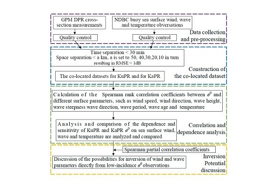
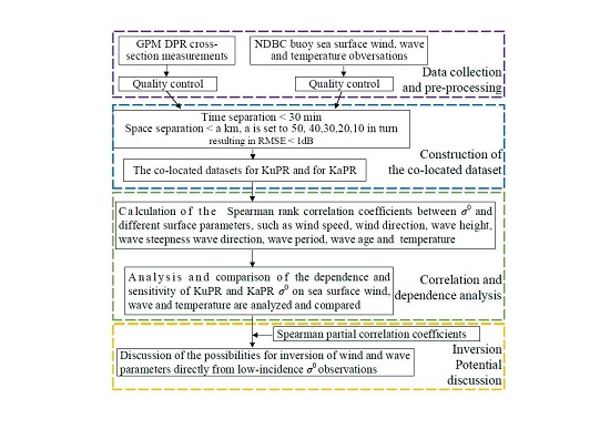
3.1. Overview

Following Chu et al. [7], the Spearman rank correlation coefficient is used to investigate the dependence and sensitivity of σ0 on surface conditions. 
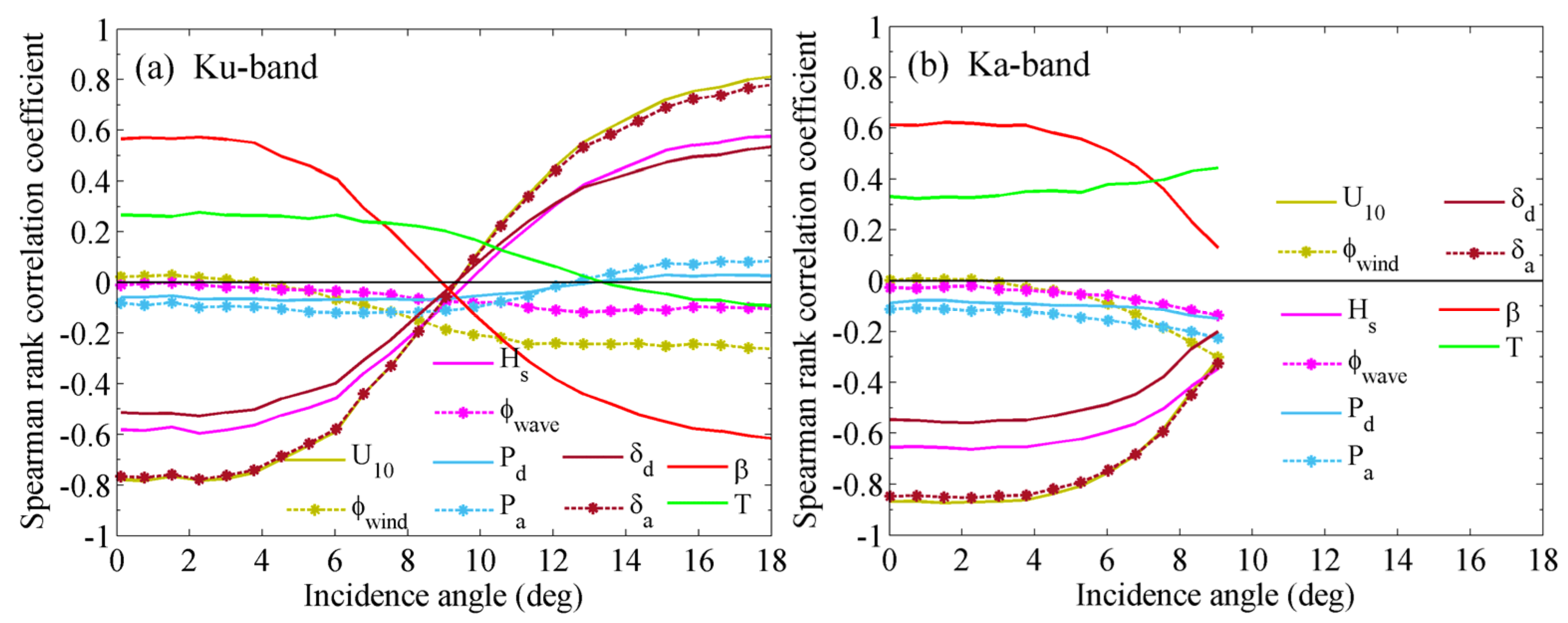
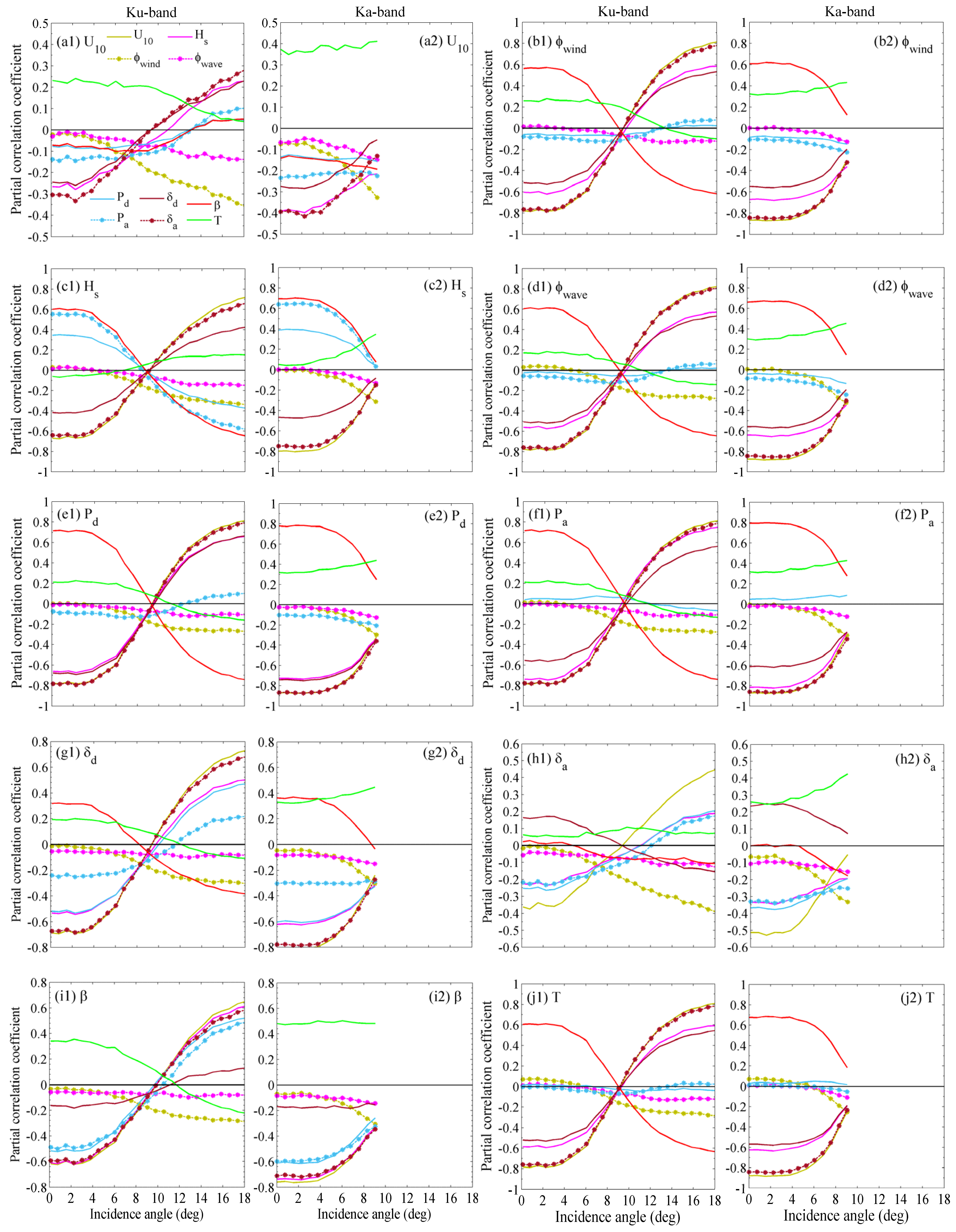
Figure 3 shows the Spearman rank correlation coefficients between σ0 and surface wind, wave and temperature parameters, including 10-m wind speed (U10), relative wind direction (ϕwind), significant wave height (Hs), relative wave direction (ϕwave), dominant wave period (Pd), average wave period (Pa), dominant wave steepness (δd), average wave steepness (δa), real wave age (β) and sea surface temperature (T). The relative wind direction is defined as ϕwind = φwindφradar, where φwind is the direction the wind is coming from and φradar is the satellite azimuth look direction, both with respect to the North. ϕwind = 0 corresponds to an upwind observation for which the wind is blowing toward the radar. In the correlation coefficient calculation, ϕwind is normalized to the range of 0–90° assuming that the backscattered signals are isotropic. ϕwave = φwaveφradar is defined similarly. The dominant wave steepness and average wave steepness are respectively defined as δd = Hs/λd, δa = Hs/λa, where λd and λa are the peak wavelength and average wavelength estimated from the corresponding wave period using the dispersion relation for waves in deep waters:
ω d 2 = g k d ω a 2 = g k a
where ω = 2π/P and k = 2π/λ are the angular frequency and the wavenumber, g is the acceleration due to gravity. Real wave age is defined as β = Cp/U10, where Cp is the phase velocity of the dominant wave, and Cp = λd/Pd.
Figure 3a shows, for KuPR, the correlation coefficients near 0° and near 18° are opposite in sign for nearly all of the parameters. It is because the correlations between σ0 and sea surface roughness near nadir and near 18° are reversed. At nadir, the rougher the sea surface is, the less signals can be returned to the radar. Conversely, at incidence angles near 18°, the radar backscatter increases with sea surface roughness. The transition point is around 9.2°, where σ0 loses its dependence on wind speed as in here the sum of the quasi-specular reflection and Bragg scattering does not vary with the surface roughness [20,21]. It can be regarded as the transition point between the quasi-specular and Bragg regions [21]. Figure 3b shows, for KaPR, at the incidence angles of 0°–9°, the correlation coefficients for every parameter are more significant than the KuPR counterparts, indicating that the Ka-band backscatter is more sensitive to the surface conditions. The Ka-band transition point is estimated to be at 10–12°, which is consistent with the result obtained by Tanelli et al. [8] based on the airborne radar data.
Whether for KuPR or KaPR, R(σ0,U10) and R(σ0,δa) are the two largest among the given parameters indicating that the ocean surface roughness is the most strongly correlated with wind speed and average wave steepness. Here, R(x, y) represents the Spearman rank correlation coefficient between x and y. On the contrary, dominant wave direction, dominant wave period and average wave period are the three parameters that have the least impact on KuPR and KaPR σ0. This is probably attributed to the constant presence of background swell. Researches have shown that the correlations are almost absent when the ocean surface is dominated by swell [7]. Moreover, considering wavelength can be calculated from wave period using the dispersion relation, they have the same level of correlation with σ0 (figures not shown). The remaining parameters are all more or less related to the sea surface roughness, and have some effect on σ0 that cannot be ignored under certain incidence angles. Below, we will discuss in detail the effects of wind speed, wind direction, wave height, wave steepness, wave age and sea surface temperature on low-incidence Ku- and Ka-band radar backscatter.

3.2. Wind Speed and Wind Direction

In general, both the KuPR σ0 and KaPR σ0 are most significantly correlated with wind speed. This makes sense because the sea surface roughness, which is primarily contributed by surface waves a few centimeters to a few meters long, is directly related to wind speed. Fully empirical model functions relating Ku-band σ0 to wind speed have already been established using a co-located PR and TMI dataset [1]. The functions suggest that the wind speed dependence of PR σ0 (in dB) at a selected incidence angle can be modeled as the sum of an exponential (important at low winds) and a linear (dominated at moderate to high winds) [1]. Here, the similar functions relating KuPR σ0 and even KaPR σ0 to wind speed are developed using the co-located datasets described in Section 2, and shown in Figure 4a and Figure 4b, respectively. For each incidence angle, the sample σ0 measurements are averaged within 0.1-m/s-wind-speed and ±0.1°-incidence-angle bins. Figure 4a shows for KuPR, the results are consistent with those obtained from PR data in previous studies (e.g., [1,7]), indicating that the Ku-band σ0 decreases monotonically near nadir, increases monotonically near 18°, and first increases then decreases with a low sensitivity to wind speed between 5° and 12° with increasing wind speed. The KuPR σ0 is nearly insensitive to wind speed near 12° for wind speeds about >4 m/s. From Figure 4b, it can be seen that the variations of KaPR σ0 with wind speed are similar to KuPR at the incidence angles of 0.1°–9.1°, but the Ka-band radar backscatter is more sensitive to wind speed, especially at moderate to high wind speeds. For example, at the incidence angle of 9.1°, the KaPR σ0 reduces by 2.2 dB with wind speed increasing from 4 m/s to 20 m/s, while for KuPR, the reduction is only 1.1 dB.
The standard deviations of the KuPR and KaPR σ0 measurements in each wind speed and incidence angle bin are also calculated, and shown in Figure 4c,d, respectively. In the same bin, the standard deviations of KuPR σ0 and KaPR σ0 are approximately on the same order of magnitude. But collectively, the standard deviations of KaPR σ0 are slightly more divergent. For all incidence angles, the standard deviations at moderate wind speeds (approximately 5–15 m/s) are relatively stable and small. At higher wind speeds, bin standard deviations become more divergent. At lower wind speeds, the standard deviations show an rapidly increasing trend with decreasing wind speed. Variations in σ0 within a bin probably result from: (1) inherent noise in the radar measurements, (2) variations of the true σ0 within the finite wind speed and incidence angle ranges defined by the bin, which imply the effect of the presence of long waves that is particularly significant at low wind speeds, (3) misbinning owing to the uncertainty of buoy wind speed, especially at weak winds when technical problems exist in buoy measurements. At very low wind speeds, both buoy error and the high sensitivity of σ0 to wind speed contribute to the increased uncertainty in the mean σ0. The more divergent standard deviations of KaPR σ0 may also be due to the higher sensitivity of KaPR σ0 to wind speed.
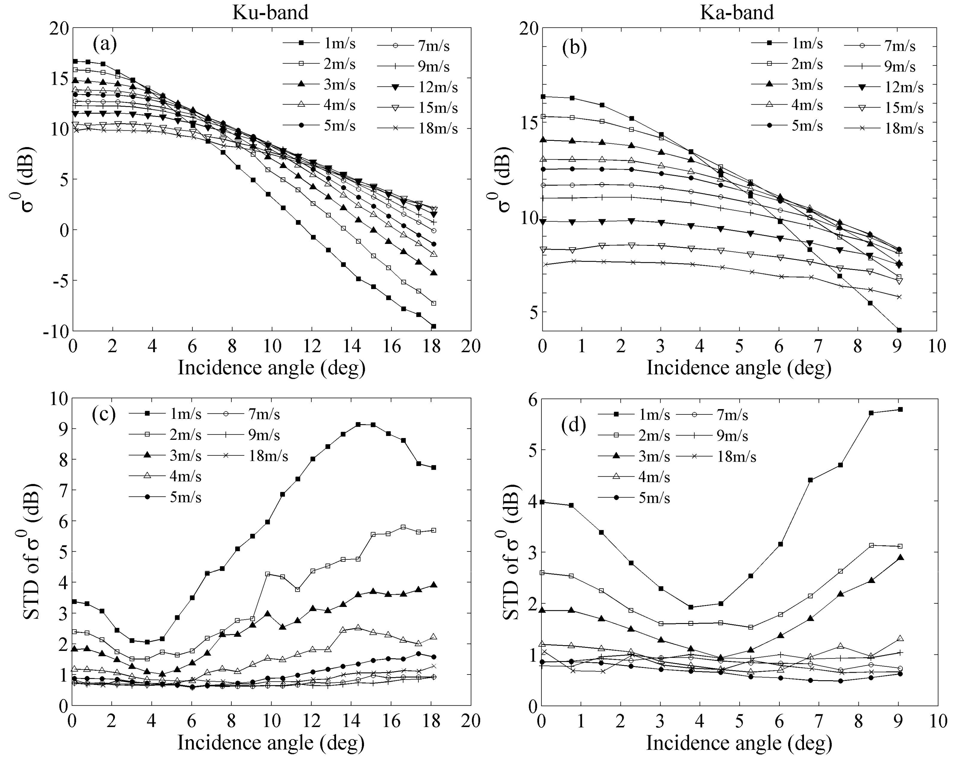
Figure 5a shows the mean values of binned KuPR σ0 as functions of incidence angle for different wind speeds. The 25 different incidence angles are from 0.1° to 18.1°, and the bin width is about 0.2°. The wind speed bin width is set to 1 m/s. As previously published, the mean KuPR σ0 decreases monotonically with increasing incidence angle for all wind speeds; the sensitivity of KuPR σ0 to incidence angle decreases with increasing wind speed. Near nadir, lower wind speeds result in larger KuPR σ0, while near 18°, the opposite is true, and thus in the middle, the KuPR σ0 exhibits low sensitivity to wind speed. The standard deviations of binned KuPR σ0 with respect to incidence angle for different wind speeds are shown in Figure 5c. For all wind speeds, the standard deviations firstly decrease, then increase with increasing incidence angle. The minimum occurs at an incidence angle θm between 4–11°, implying in here σ0 not only exhibits low sensitivity to wind speed but also an overall low variability. The angle θm shows an increasing trend with increasing wind speed up to 7 m/s, followed by a saturation toward about 11° for higher wind speeds. Moreover, the magnitudes are smaller at nadir than at 18° for light wind speeds, but above 5 m/s, the values are similar. This may be attributed to the fact that the effect of the presence of long waves is more significant at 18° at light winds [5]. Figure 5b,d show, respectively, the mean values and standard deviations of binned KaPR σ0 as functions of incidence angle for different wind speeds. The 13 different incidence angles are from 0.1° to 9.1°. The results similar to KuPR in this incidence angle range can be obtained. The above results are mainly consistent with those of several previous studies (e.g., [1,5,8]).
It is suggested in Figure 3 that, whether for KuPR or KaPR, the correlation between σ0 and wind direction is becoming increasingly significant when incidence angle exceeds about 5–6°.
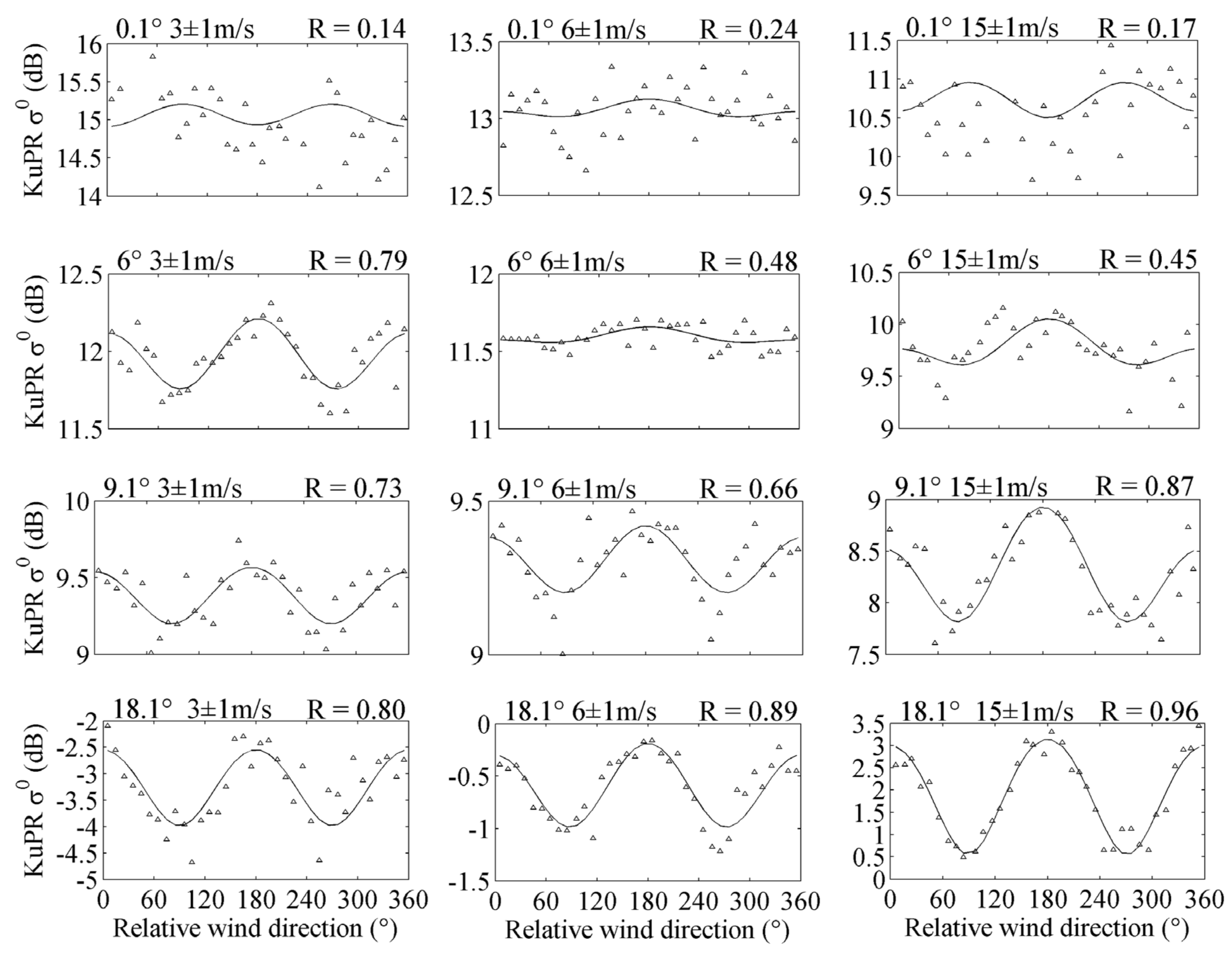
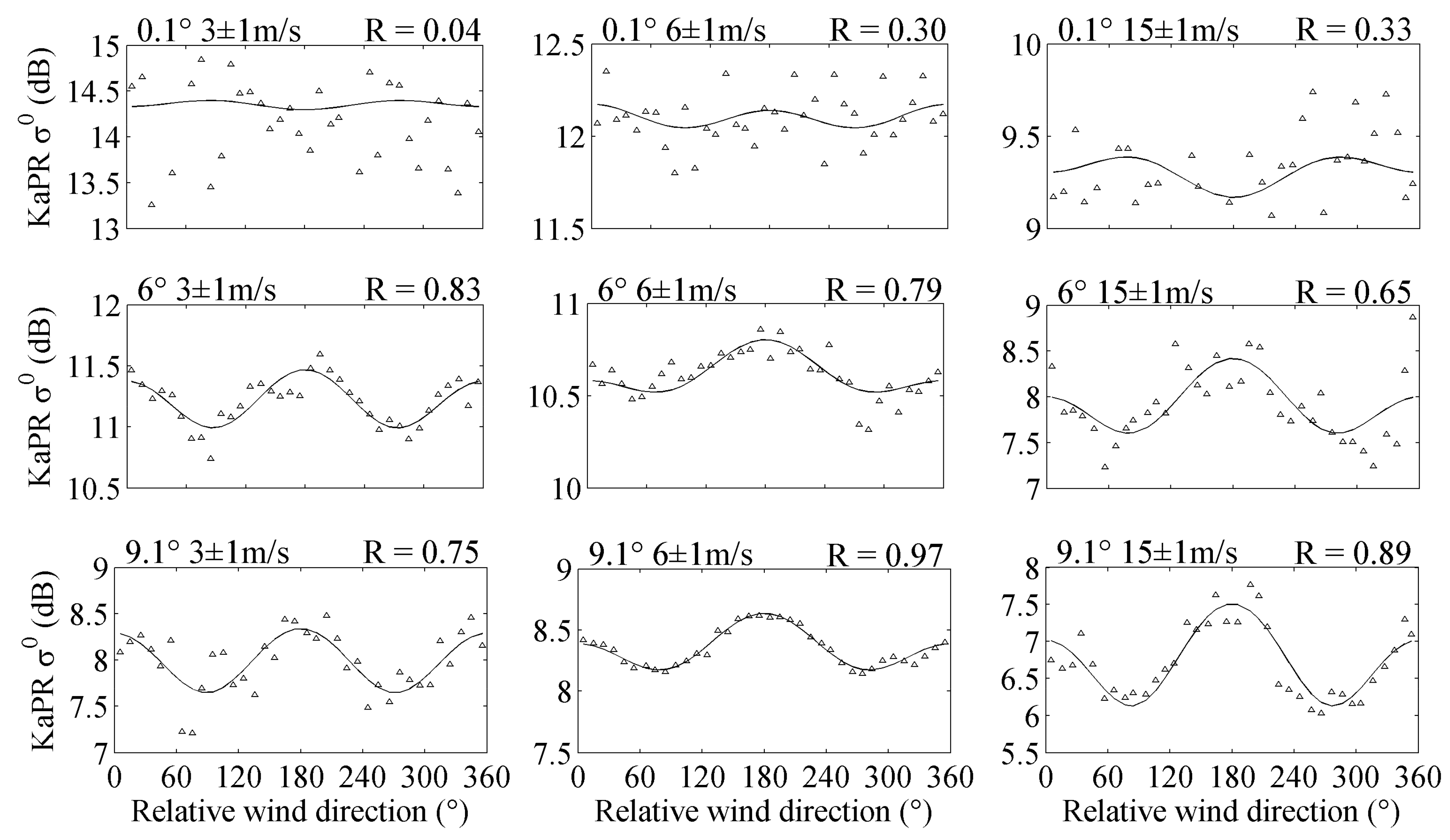
 Figure 6 and Figure 7 display respectively the variations in KuPR and KaPR σ0 with wind direction at different wind speeds and incidence angles. The measured σ0 is averaged within 10° relative wind directions, ±1 m/s wind speeds, and ±0.1° incidence angles bins. The 3σ (3 times standard deviation) filter is applied within each bin to eliminate earlier measurements. As shown, the directional dependence of σ0 becomes obvious, and shows clear biharmonic behavior above approximately 6°. This can be explained by non-Gaussian assumption and Bragg scattering theory. The sea slope distribution in the open ocean is not Gaussian (e.g., the Gram–Charlier distribution), and this is one reason for the directional variations of σ0 [6,18]. The Bragg scattering component, which becomes more and more important with incidence angle, can also contribute to the directional variations. Based on previous researches, this biharmonic behavior can be empirically modeled by a second-order Fourier series as: σ0 = a0 + a1cos(ϕwind) + a2cos(2ϕwind), where σ0 is in natural units (not in dB), a0, a1 and a2 are wind speed and incidence angle dependent coefficients [6]. Empirical curves from the least squares regression fits are shown in Figure 6 and Figure 7 as solid lines to better display the trend. It can be seen that the directional dependence of σ0 increases with incidence angle, and first decrease than increase with wind speed.
Both for KuPR and KaPR, σ0 shows a considerable scatter with very small correlation coefficients R, and the wind direction dependence is quite weak for all wind speeds at low-incidence angles (about <5°). At 0.1°, there is no wind directional signal above the noise level, which is possibly due to the fact that the directional signals are so small that they are submerged in the large fluctuation of σ0 (about >0.8 dB, see Figure 5c,d). At about 4.5°, the modeled directional modulation is less than 0.5 dB at a 15-m/s wind speed. Above 5°, the amplitude of the modeled peak-to-peak σ0, defined as the difference between the maximum σ0 and the minimum σ0, increases dramatically with incidence angle increasing. Moreover, the KaPR σ0 is more sensitive to wind direction. At 9.1°, a 15-m/s wind will produce peak-to-peak azimuth modulation of about 1.1 dB for KuPR and 1.4 dB for KaPR. Furthermore, for KuPR, all peak-to-peak σ0 values are larger than 0.5 dB (half order of the σ0 bias) at 13.5°. At 18.1°, the modeled azimuth modulation exceeds 0.8 dB for all wind speeds, and reaches about 2.5 dB at a 15-m/s wind speed. These results are fairly consistent with those obtained from [6] and [7].
The observations show that the maximum σ0 values coincide with the radar beam directed parallel to the upwind/downwind directions, and the minimum σ0 values correspond with the radar beam crossing the wind direction. Overall, at low-incidence angles, σ0 is slightly larger in the downwind direction than in the upwind direction. Such signatures of the microwave backscatter from sea surface can be explained by the anisotropic and asymmetric growth of short surface waves. 
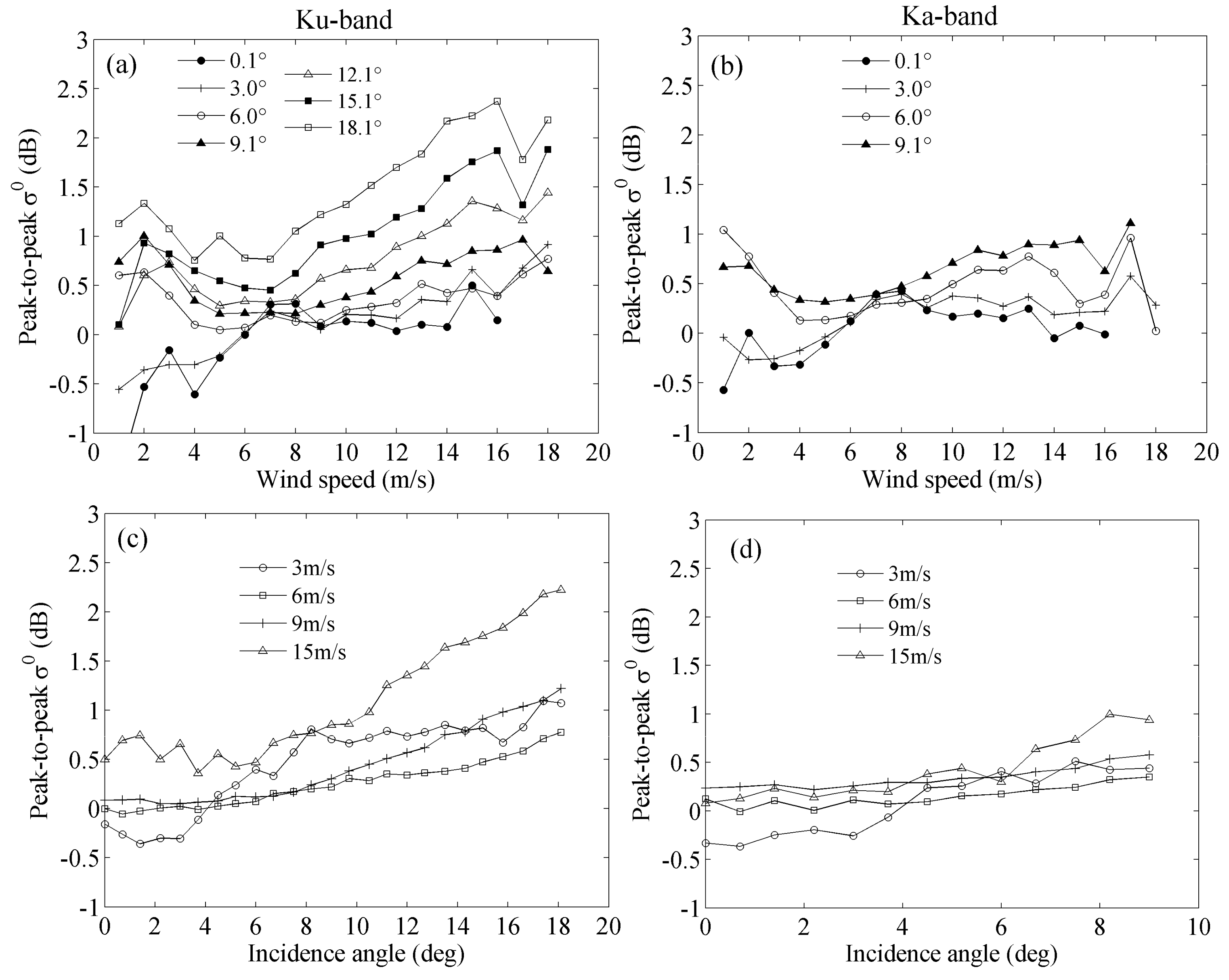
Figure 8 depicts the change trend of KuPR and KaPR peak-to-peak σ0 with wind speed and incidence angle. Here, the peak-to-peak σ0 is defined as (σ0(upwind) + σ0(downwind) – 2σ0(crosswind))/2. As shown, whether for KuPR or KaPR, there is a change in behavior of the peak-to-peak directional signal at a critical wind speed of about 4 to 6 m/s. Below this wind speed range, the absolute magnitude apparently decreases with increasing wind speed. This might be due to the fact that there is significant uncertainty in mean σ0 that decreases with wind speed at low winds (see Figure 4c,d). Then it increases for higher wind speeds. For all wind speeds, the magnitude is positive and increases monotonically with increasing incidence angle above about 6°. At lower incidence angles, it is rather small, and there are negative values at low winds probably due to the large uncertainty in mean σ0 as well.

3.3. Wave Height, Wave Steepness and Wave Age

Wind alone is insufficient to describe σ0, especially at low winds. To better interpret σ0, the effects of wave need to be included. The Spearman partial correlation coefficients between σ0 and wave parameters controlled by wind speed are calculated (see Figure 20a1 for KuPR and Figure 20a2 for KaPR), indicating significant wave height (Hs) and wave steepness (both δa and δd) have much larger effects on the residual σ0. The correlation between σ0 and Hs is relatively good (see Figure 3) and the direct relationship can be established. 
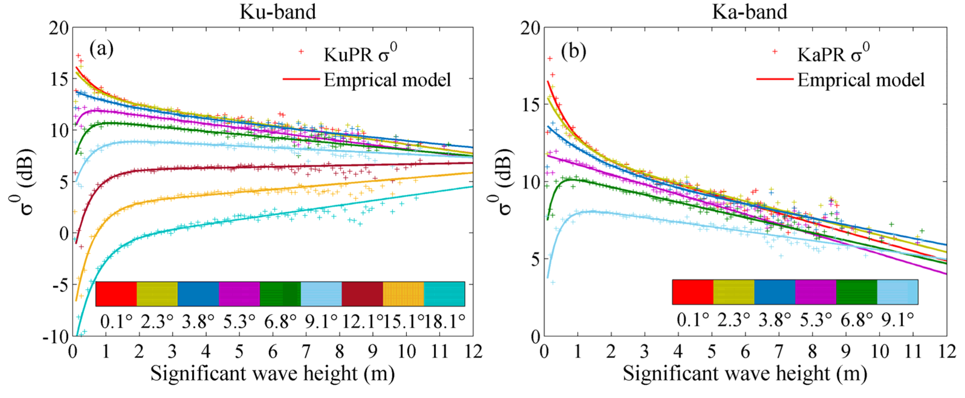
Figure 9a displays the KuPR σ0 measurements averaged within 0.1-m-significant-wave-height bins with respect to significant wave height for selected incidence angles and the corresponding empirical model functions, each of which can be expressed as the sum of an exponential term and a linear term, similarly to the wind speed model. This figure shows a similar trend to that in Figure 4a, but the variation range of σ0 is apparently narrower at each incidence angle. This means the effect of significant wave height on σ0 is smaller than that of wind speed. The mean values of binned KaPR σ0 and the model predictions are shown in Figure 9b, as functions of significant wave height for incidence angles of 0.1°-9.1°. Similar results can be obtained. Beyond that, the KaPR σ0 is more sensitive to wave height. For instance, at 9.1° incidence angle, the KaPR σ0 reduces by 1.2 dB with significant wave height increasing from 2 m to 6 m, while for KuPR, it is only 0.6 dB.
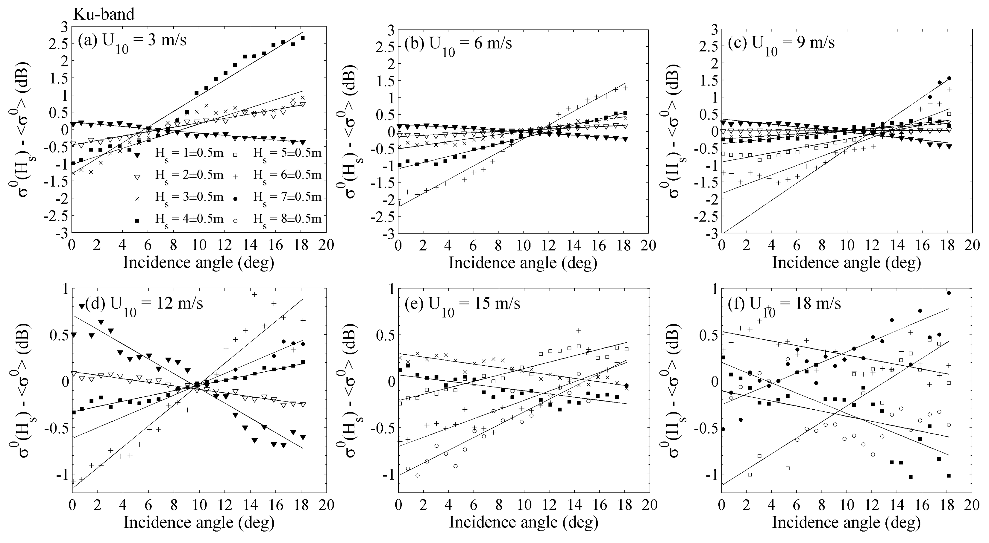
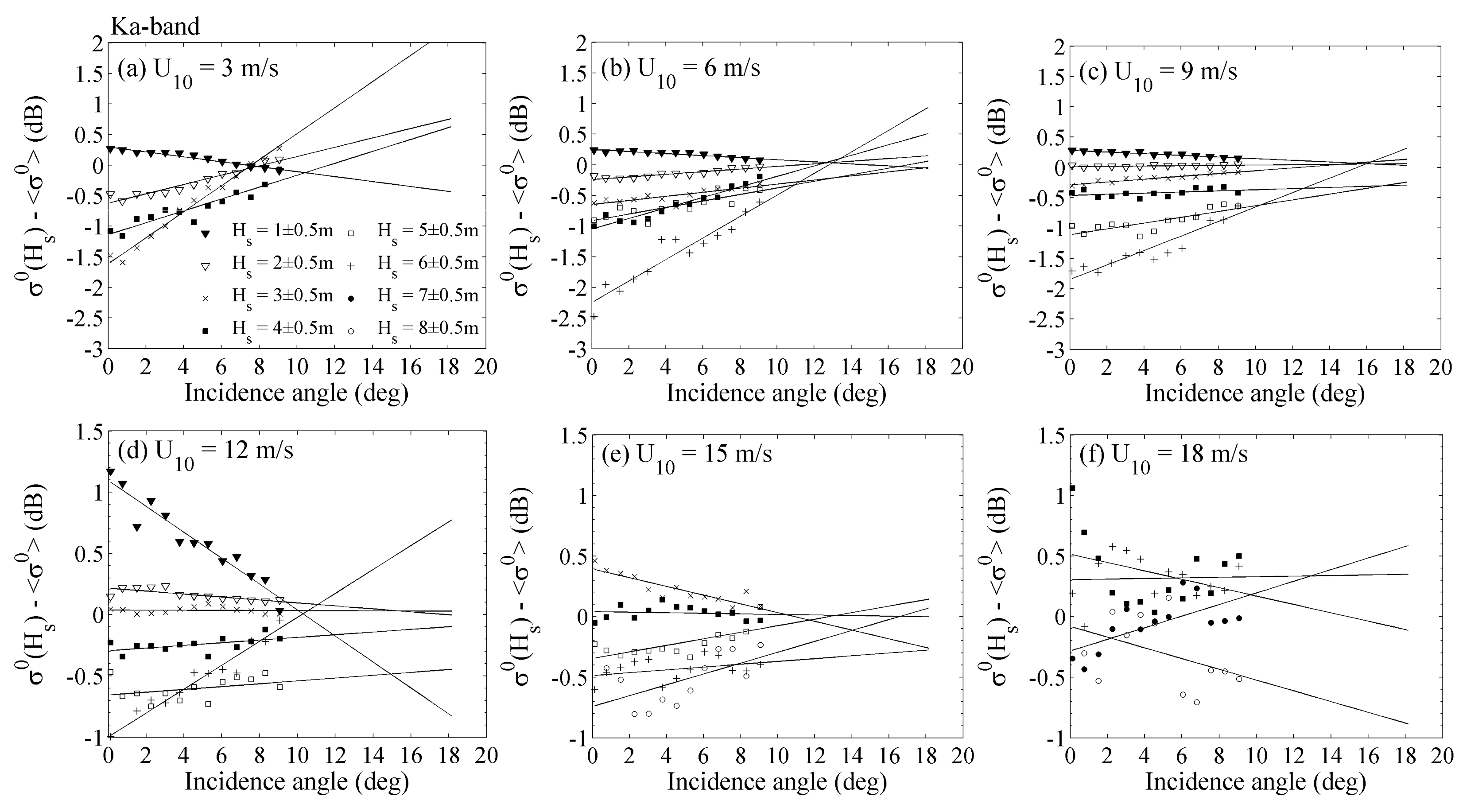
Figure 10 shows the magnitude of the difference between averaged KuPR σ0 associated to a 1-m class of Hs and the averaged value over all Hs with respect to incidence angle at six selected wind speeds of 3, 6, 9, 12, 15 and 18 m/s. The 1-m/s wind speed bin is used. The solid lines are the linear least squares fits to better display the trends. For low to moderate winds (about <15 m/s), behavior of the difference as a function of significant wave height is clear. At lower Hs, the magnitude of the difference decreases with increasing angle, whereas for higher Hs, it exhibits the opposite trend. The critical Hs becomes larger as the increase of wind speed (e.g., it is a value between 1 m and 2 m at 3 m/s, but between 4 m and 5 m at 15 m/s). The overall picture shows at a given wind speed, all curves associated to different Hs classes roughly intersect at a particular incidence angle, denoted θz. The above-described characteristics indicate that σ0 decreases near nadir and increases near 18° with increasing significant wave height. This is because that higher Hs results in more significant tilting effect that modifies the local incident angle, and hence reduces the backscattering intensity near nadir and increases the backscatter near 18°. However, for high winds (e.g., 18 m/s), most of these characteristics are missing except for the nearly linear trend of the magnitude with incidence angle. This may be attributed to the fact that the impact of significant wave height on σ0 decreases with increasing wind speed, and becomes so small that it is submerged in the fluctuation of σ0 at high winds.
The magnitude of the difference between σ0(θ, U10, Hs) and σ0(θ, U10) of KaPR with respect to incidence angle for various 1-m Hs classes at the six selected wind speeds and the corresponding fitting lines are displayed in Figure 11. In contrast with KuPR, one obvious difference for KaPR shown in Figure 11 is that all curves (linear least-squares fits) associated to the different Hs classes do not appear to intersect at one point at a given moderate wind speed (e.g., 6, 9, 12 m/s). But this remains questionable considering the total trend of the magnitude of the difference over the incidence angle range of 0–18° is doubtful as the KaPR σ0 measurements can only cover the 0–9° incidence angle range.
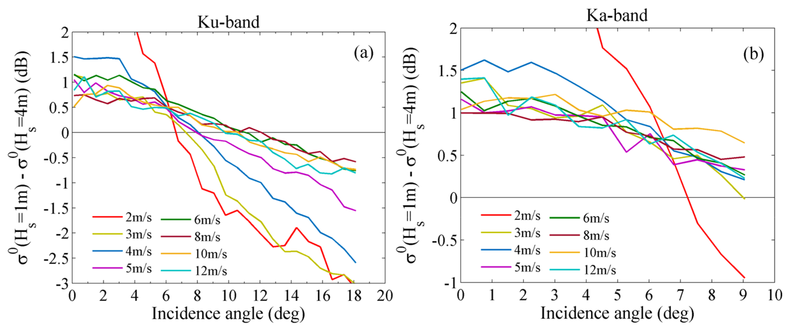
The magnitude of the difference of KuPR σ0 between low Hs (1 m) and high Hs (4 m) conditions is shown in Figure 12a as a function of incidence angle for different wind speeds from light to moderate winds. The blank at high winds is due to the scarcity of data in this region. As shown, the magnitude is positive at low-incidence angles, and decreases to become negative at higher incidence. For a given wind speed, the magnitude reaches zero at the incidence angle θz between 6°–12°. Similar to θm, the angle θz first increases with wind speed increasing up to 6–8 m/s, then shows a saturation trend at higher winds. Around the critical angles, the mean σ0 is insensitive to significant wave height variations. At moderate winds, the impact of the existence of large waves with high Hs on radar backscatter is not significant since the observed differences are within the uncertainty of the radar (±1dB). But at very low winds, the differences are quite high near nadir and near 18°, and the impact of significant wave height on σ0 is particularly remarkable. Moreover, the absolute magnitudes are smaller near nadir than near 18° for low wind speeds (about <5 m/s), which might explain the results obtained from Figure 5 above. The relative magnitude of KaPR σ0 for extreme conditions is shown in Figure 12b. Compared with KuPR, the critical angles for KaPR appear to be slightly rightwardly shifted, and the differences near nadir are larger, e.g., the differences at nadir are within 1–1.5 dB at moderate winds. This again emphasizes that the impact of significant wave height on KaPR σ0 is more obvious.
The KuPR σ0 and KaPR σ0 are also closely correlated with wave steepness (including both δa and δd). As found in Figure 3, R(σ0, δa) is much larger than R(σ0, δd), indicating that the dependence of σ0 on δa is much more remarkable. This is possibly attributable to the fact that δa is an integrated property like Hs, whereas δd is an unstable quantity and less robust [7]. Moreover, R(σ0, δa) is only slightly smaller than R(σ0, U10). Moreover, in some cases (e.g., pure-swell sea), R(σ0, δa) can be greater than R(σ0, U10) [7]. The direct relationship between
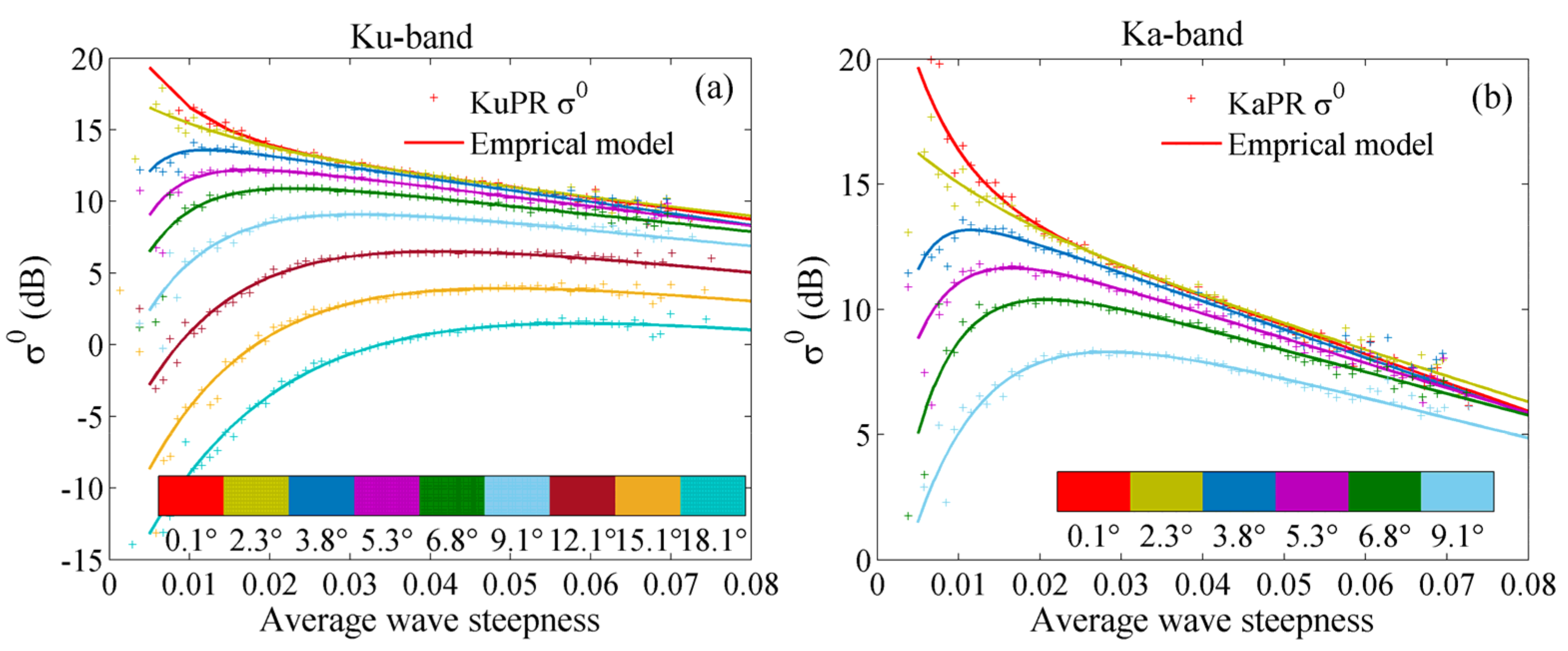
 σ0 and δa is established and shown in Figure 13. The wave steepness bin width is set to 0.001. The blank area at extremely low steepness is due to the scarcity of data in this region. Similarly, the empirical relation can be modeled as the sum of an exponential term and a linear term. The curves show similar shapes to those in Figure 4 and Figure 9. Likewise, the KaPR σ0 is more sensitive to wave steepness. At the incidence angle of 9.1°, the KaPR σ0 reduces by 1.8 dB with average wave steepness increasing from 0.03 to 0.06, while for KuPR, the reduction is only 1.1 dB.
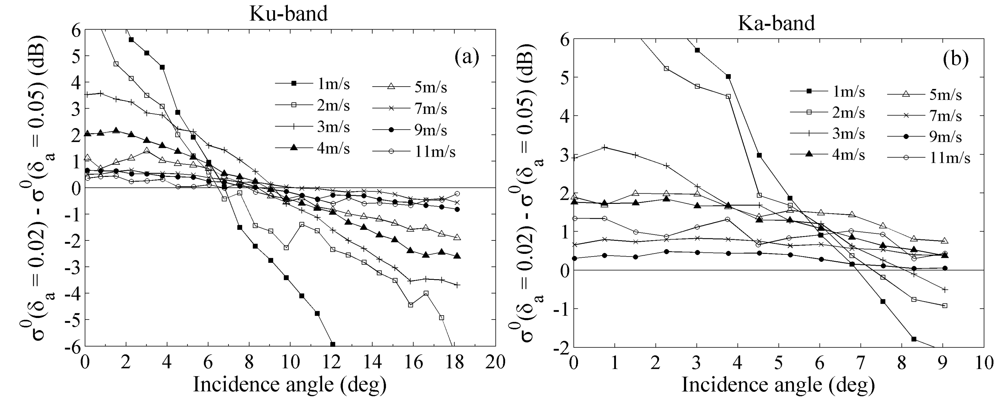
To further evaluate the effect of δa, the magnitude of the difference of σ0 between two typical wave steepness values (δa = 0.02 and δa = 0.05 ) is shown in Figure 14 as functions of incidence angle for light-to-moderate wind speeds. The behavior of the difference is similar to that in Figure 12. For all wind speeds, the magnitude is positive at low-incidence angles, and decreases to reach a negative value at higher incidence angles. The zero-crossing points are between 6–12°, and show an increasing trend at lower wind speeds (about <7m/s), followed by a saturation trend for higher wind speeds. With the exception of the specific incidence angles, differences in σ0 due to different δa levels are significant, especially at low wind speeds (about <5m/s). The difference in KaPR σ0 is generally larger than the KuPR counterpart. In addition, however, the difference in σ0 between two typical wave steepnesses is much larger than that between two typical significant wave heights at low wind speeds.
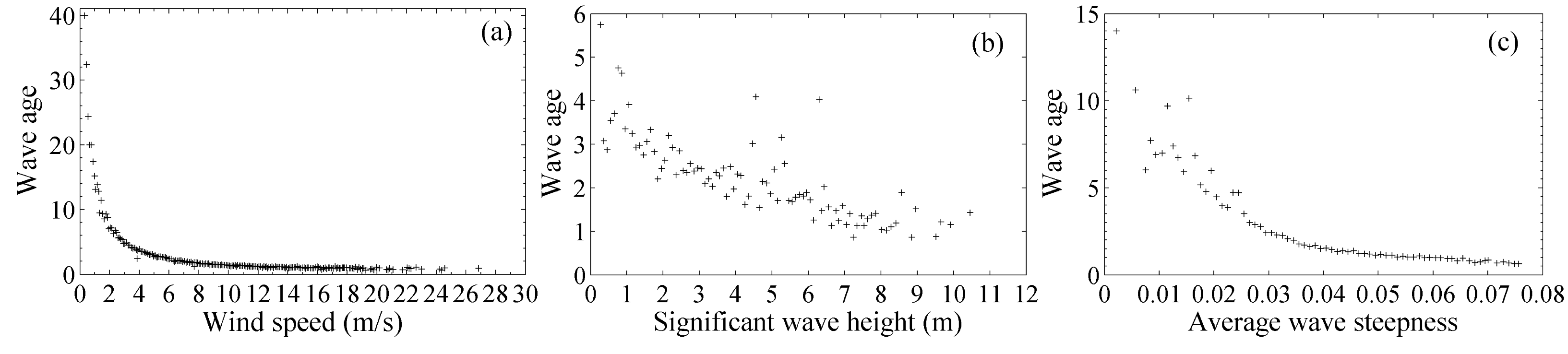
Real wave age (β) is a parameter commonly used to characterize the wave maturity state. The larger the wave age, the more developed the wave, and the smoother the sea surface. That is, wave age is negatively correlated with surface roughness. Thus near nadir, the radar power is positively related to wave age, whereas near 18°, they are negative correlated, as shown in Figure 3. Figure 15a–c show the averaged β over respectively the same wind speed, significant wave height and average wave steepness in the present dataset. As shown, wave ages are very high at low wind speeds. This may be one reason for the rapid change of σ0 near nadir and near 18° in this region (see Figure 4). For low Hs and low δa (see Figure 9 and Figure 13), the situations are similar except that the lines are less steep partly for the relatively small wave age. In addition, the curves at low Hs in this study are more steep than those in [7] as the wave age in the present dataset is larger (see Figure 6a in [7] for a comparison). These further confirm that the impact of sea state on σ0 is significant, particularly at low wind speeds.
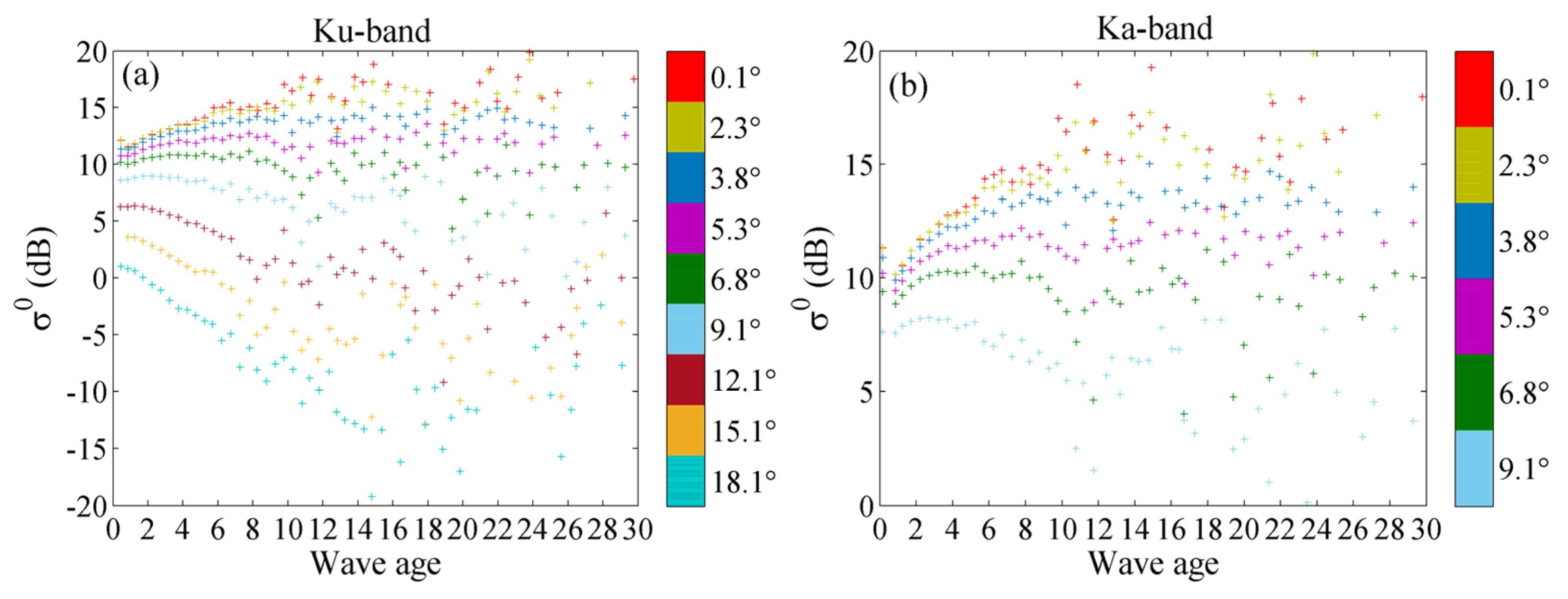
The binned mean KuPR σ0 and KaPR σ0 with respect to wave age for selected incidence angles are shown in Figure 16a,b, respectively. For KuPR, σ0 exhibits an increasing trend near nadir and a decreasing trend near 18°, and first increases then decreases in the middle incidence angles with increasing wave age. For KaPR, similar trends can be seen for the incidence angles of 0.1–9.1°. Moreover, the sensitivity of KaPR σ0 to wave age does not show apparent difference with that of KuPR σ0.

3.4. Sea Surface Temperature

The radar cross section σ0 is representative of the sea surface roughness at the scale of capillary gravity waves, which are not only dominated by winds and modulated by long waves, but also influenced by some secondary factors such as sea surface temperature and sea surface salinity. The variation of surface roughness caused by sea surface salinity is very small, thus we neglect its influence and only investigate the effect of sea surface temperature [22]. 
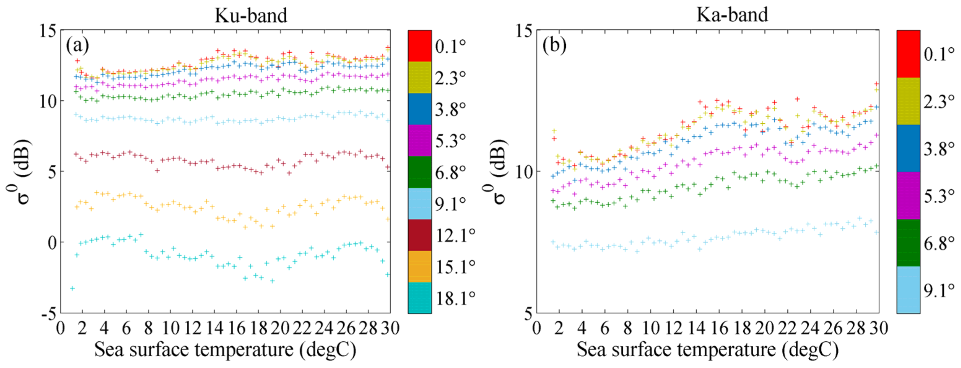
Figure 17 shows the variations of KuPR σ0 and KaPR σ0 with sea surface temperature for selected incidence angles. As shown in Figure 3 and Figure 17, at relatively low-incidence angles, σ0 is weakly and positively correlated with sea surface temperature, and shows a slightly increasing trend with increasing sea surface temperature. The KaPR σ0 is slightly more sensitive to sea surface temperature. At higher incidence angle, only for KuPR, the correlation becomes smaller, and σ0 has no obvious variation trend. Moreover, the impact of sea surface temperature on σ0 is much more significant at low wind speeds (see Figure 18 as an example).
These results obtained in the present dataset are possibly attributed to the comprehensive effect of the factors described below. Physically, sea surface temperature affects the dielectric constant of water, surface tension, and water kinematic viscosity, three parameters which potentially may influence the observed radar backscatter from the ocean [22]. As sea surface temperature increases, the dielectric constant increases, and thus σ0 increases. This perturbation is more remarkable at Ka-band [23]. For example, at 0° incidence angle, the Ka-band specular reflectivity increases from 0.48 to 0.56, and thus the Ka-band σ0 increases 0.7dB when sea surface temperature increases from 0 to 30 °C. In contrast, the Ku-band specular reflectivity increases from 0.59 to 0.61 and the Ku-band σ0 only increases 0.2dB. As sea surface temperature decreases, the surface tension increases. We believe that this effect can reduce the surface roughness at low winds [22]. Moreover, this, coupled with the impact of constant presence of background swell, causes the relatively large perturbations of σ0 with sea surface temperature at low winds. Viscous dissipation is directly proportional to the kinematic viscosity of sea water. As sea surface temperature increases, the kinematic viscosity becomes smaller, and then ripples dissipation decreases.

4. Discussion

4.1. Physical Interpretation of Higher Sensitivity of KaPR Backscatter

The dependence and sensitivity of KuPR and KaPR σ0 on surface wind, wave and temperature parameters have been systematically analyzed and compared in Section 3. It can be found that the KaPR σ0 is more sensitive to surface conditions. This should be caused by the smaller wavelength of Ka-band. Here, the physical interpretation for the higher wind speed sensitivity of the KaPR σ0 is deeply discussed. For an isotropic sea surface of Gaussian statistics, near-nadir σ0 can be written as [1,16]:
σ 0 θ = R eff 2 s 2 sec 4 θ exp tan 2 θ s 2
where θ is the incidence angle, |Reff|2 is effective nadir reflection coefficient and s2 is the radar filtered mean square slope. |Reff|2 and s2 are both functions of wind speed. |Reff|2 can be calculated by using the formula given by Valenzuela [16]. Moreover, it is related to the energy spectral density of the surface roughness. s2 can be obtained by integrating the function of surface roughness spectrum from zero to an upper bound cutoff wave number. The cutoff wave number reported in literature is within the range of a tenth to half of the radar wave number [24]. Here, the ratio of 1/5 and the Hwang spectrum [24,25] are selected to calculate |Reff|2 and s2. By varying U10 from 1 to 25 m/s in steps of 0.1 m/s, a dataset of |Reff|2 as functions of U10 is created. By using the non-linear least squares method, we can obtain:
R eff Ku 2 = 0.2179 exp ( 0.0179 U 10 ) 0.0109 U 10 + 0.3876 R eff Ka 2 = 0.2032 exp ( 0.0767 U 10 ) 0.0159 U 10 + 0.7485
where R eff Ku 2 and R eff Ka 2 are the effective nadir reflection coefficients for Ku-band and for Ka-band, respectively. Similarly, we can obtain:
s Ku 2 = 0.0057 + 0.002 U 10 + 0.01121 lg U 10 s Ka 2 = 0.0064 + 0.0028 U 10 + 0.0126 lg U 10
where s Ku 2 and s Ka 2 are the filtered mean square slopes for Ku-band and for Ka-band, respectively. Then the differentiation of (2) with respect to wind speed can be calculated. Figure 19 shows the wind speed dependence of the derivative of σ0 with respect to wind speed at 0° incidence angle. It can be seen that the sensitivity of σ0 to wind speed decreases with wind speed increasing. Moreover, the wind speed sensitivity of KaPR σ0 is higher than that of KuPR σ0, and the difference increases with wind speed.

4.2. Wind and Wave Inversion Potential of Low-Incidence σ0

Figure 20 shows the Spearman partial correlation coefficients between σ0 and different surface parameters, with the effect of controlling variable removed. Based on Figure 20 and the analysis in Section 3, the potential for inversion of wind and wave parameters directly from low-incidence σ0 is discussed. In general, the main parameters (wind speed, wave steepness, etc) can be retrieved from both the KuPR and KaPR σ0 measurements under specific incidence angles with necessary auxiliary information. The smaller wavelength of KaPR makes its σ0 more sensitive to surface conditions. This facilitates the retrieval of surface parameters. However, the smaller wavelength also implies that KaPR has higher sensitivity to tropospheric conditions, and rain will generally make acquisitions unexploitable.
For wind speed, it can be directly retrieved from pointwise σ0 near nadir, whereas near 18°, wind direction information is needed. In the middle-incidence angles (e.g., 5–12°), the retrieval of wind speed from a single σ0 cannot be recommended. At this point, a fieldwise approach, such as the one reported by Li et al. [26], might work. Some auxiliary parameters would help to improve the performance of the retrieval of wind speed, especially low wind speed. Wave steepness δa is the preferred. This confirms the statements made by Hwang et al. [27] and Quilfen et al. [28] that sea state steepness should be included in wind speed retrieval at low-incidence angles. Significant wave height is of secondary importance. This explains a previous finding reported by Gourrion et al. [29] that the introduction of significant wave height enhances the accuracy of altimeter low wind speed estimation. Moreover, to further improve the performance of low wind speed retrieval, particularly near nadir, sea surface temperature information is needed. Wind direction should be taken into account above 13.5° for KuPR. For KaPR, this angle is even smaller. Wind direction could be retrieved from multi-azimuthal looks of σ0, e.g., acquired by a radar with multiple fan-beam side-scanning antennas illuminating sea surface at different azimuth angles (e.g., ASCAT, the Advanced Scatterometer) or a conical scanning radar (e.g., QuickSCAT, the Quick Scatterometer).
The relationship between σ0 and significant wave height is strongly affected by most parameters (e.g., wind speed, wave steepness and wave age, etc). Therefore, various auxiliary information should be taken into account for the retrieval of wave height. Wave direction rarely affects the relationships between σ0 and other variables. The introduction of any other parameter cannot effectively improve the performance of wave direction retrieval. These imply that it is hardly possible to estimate wave direction directly from the pointwise σ0 measurements. For wave direction retrieval, the fieldwise approaches, such as conventional spectral analysis techniques, might work. The correlation between σ0 and wave period can be effectively enhanced with the control of wave height, wave steepness or wave age. This is consistent with the finding reported by Remya et al. [30] that the introduction of wave age is quite helpful for the altimeter wave period estimation using a genetic algorithm. Wave steepness δa shows great potential for retrieval directly from σ0 near nadir and near 18°. Moreover, an auxiliary wind speed parameter would be helpful to improve the performance of δa retrieval. Wind direction is better taken into account near 18°. The wave age effect is also significant, although it is negatively correlated with sea surface roughness. σ0 is partially correlated with most parameters with the control of wave age. Therefore, various auxiliary information, such as wind speed, wave steepness or wave period, is needed for the retrieval of wave age directly from the σ0 measurements at low-incidence angles.

5. Conclusions

Based on the collocations of GPM DPR normalized radar cross section measurements and NDBC moored buoy sea surface observations, the dependence and sensitivity of KuPR and KaPR σ0 on surface wind, wave and temperature parameters are systematically analyzed and compared. Then the possibilities for inversion of wind and wave parameters directly from σ0 at low-incidence angles are discussed.
The relationships between σ0 and various surface parameters are investigated using correlation and dependence analysis. The results show that the KaPR σ0 is more sensitive to surface conditions than the KuPR σ0 overall. The physical interpretation for the higher wind speed sensitivity of the KaPR σ0 is discussed in detail. While for other surface parameters, similar analysis will be conducted in future work. Nevertheless, both the KuPR σ0 and KaPR σ0 are correlated with most surface parameters, such as wind speed, wave steepness, wave height and wave age, with the exception of specific transitional incidence angles. In the incidence angle range of 0–18°, the best incidence angles for pointwise retrieval of these parameters are those near nadir or near 18°. Moreover, wind direction must be taken into account when incidence angle exceeds a certain value (about 13.5° for KuPR, and even smaller for KaPR) as the effect of wind direction on σ0 becomes increasingly significant with incidence angle increasing.
Both the KuPR σ0 and KaPR σ0 are most strongly correlated with wind speed. The relationship between σ0 and wind speed at different incidence angles can be well described by the empirical model functions. Near nadir or near 18°, σ0 varies monotonically with wind speed, and wind speed can be directly retrieved from pointwise σ0. But near 18°, wind direction is better taken into account. While in the transition region, σ0 shows a nonmonotonic relationship with wind speed, the retrieval of wind speed from a single σ0 cannot be recommended. It is especially necessary to point out that there is large uncertainty in mean σ0 at low winds. Auxiliary information related to sea state is needed to improve the performance of wind speed retrieval, especially for low wind speed. Wave steepness δa is preferred. Significant wave height data are of secondary use, and real wave age information might not significant. In addition, sea surface temperature is better taken into account for low wind speed retrieval.
The KuPR σ0 and KaPR σ0 are also closely correlated with wave steepness, particularly average wave steepness δa. δa includes contributions from both the wind and sea state in describing the surface roughness. δa shows great potential for retrieval directly from pointwise σ0. To improve δa retrieval, an auxiliary wind speed parameter would be helpful. Similar to wind speed retrieval, wind direction is better taken into account near 18°, and wave age might not significantly improve δa retrieval. Assuming that δa could be obtained operationally, the wind retrieval algorithms could be better designed.
Other wave parameters, such as significant wave height, wave period and wave age, are partly correlated with σ0. It is generally more difficult to retrieve those parameters directly from pointwise σ0. For the retrieval of those wave parameters, various auxiliary information is needed, and big data algorithms, such as neural network algorithms, should be adopted. Wind direction and wave direction cannot be retrieved from pointwise σ0, and fieldwise approaches might work.
The analysis can contribute to a better understanding of how radar backscatter and surface dynamic environment interact, and provide guidance for developing inversion algorithms to infer wind and wave parameters from low-incidence measurements. This will finally provide a basis for the geophysical interpretation of the spaceborne radars of low-incidence angles, such as the just launched Ku-band wave spectrometer (CFOSAT SWIM) and the upcoming Ka-band radar interferometer (SWOT KaRin).

Author Contributions

Conceptualization, Q.Y. and C.F.; Data curation, J.M.; Formal analysis, Q.Y.; Funding acquisition, C.F.; Investigation, Q.Y.; Methodology, Q.Y. and C.F.; Project administration, J.M.; Resources, J.M.; Software, Q.Y. and C.F.; Supervision, J.Z.; Validation, C.F.; Visualization, J.Z.; Writing—original draft, Q.Y.; Writing—review and editing, J.Z.

Funding

This research was funded by the National Key R&D Program of China, grant number 2016YFC1401005 and the National Science Foundation of China, grant number 61501130.

Acknowledgements

The authors would like to thank the Goddard Space Flight Center Distributed Active Archive Center for the straightforward and rapid electronic access to the GPM DPR data. The authors would also like to thank the American National Data Buoy Center (NDBC) for providing the buoy data.

Conflicts of Interest

The authors declare no conflict of interest.

References

  1. Freilich, M.H.; Vanhoff, B.A. The relationship between winds, surface roughness, and radar backscatter at low incidence angles from TRMM precipitation radar measurements. J. Atmos. Ocean. Tech. 2003, 20, 549–562. [Google Scholar] [CrossRef]
  2. Nouguier, F.; Mouche, A.; Rascle, N.; Chapron, B.; Vandemark, D. Analysis of dual-frequency ocean backscatter measurements at Ku- and Ka-bands using near-nadir incidence GPM radar data. IEEE Geosci. Remote Sens. Lett. 2016, 13, 1310–1314. [Google Scholar] [CrossRef]
  3. Ren, L.; Pan, D.; Mao, Z.; Wang, D.; Chen, J. Simulation and evaluation for measuring directional ocean wave spectrum from SWIM on CFOSAT. In Remote Sensing of the Ocean, Sea Ice, and Large Water Regions 2010; International Society for Optics and Photonics: San Diego, CA, USA, 2010; pp. 78250D-1–78250D-11. [Google Scholar]
  4. Durand, M.; Fu, L.L.; Lettenmaier, D.P.; Alsdorf, D.E.; Rodriguez, E.; Esteban-Fernandez, D. The surface water and ocean topography mission: Observing terrestrial surface water and oceanic submesoscale eddies. Proc. IEEE 2010, 98, 766–779. [Google Scholar] [CrossRef]
  5. Tran, N.; Chapron, B.; Vandemark, D. Effect of long waves on Ku-band ocean radar backscatter at low incidence angles using TRMM and altimeter data. IEEE Geosci. Remote Sens. Lett. 2007, 4, 542–546. [Google Scholar] [CrossRef]
  6. Chu, X.; He, Y.; Chen, G. Asymmetry and anisotropy of microwave backscatter at low incidence angles. IEEE Trans. Geosci. Remote Sens. 2012, 50, 4014–4024. [Google Scholar] [CrossRef]
  7. Chu, X.; He, Y.; Karaev, V.Y. Relationships between Ku-band radar backscatter and integrated wind and wave parameters at low incidence angles. IEEE Trans. Geosci. Remote Sens. 2012, 50, 4599–4609. [Google Scholar] [CrossRef]
  8. Tanelli, S.; Durden, S.L.; Im, E. Simultaneous measurements of Ku- and Ka-band sea surface cross sections by an airborne radar. IEEE Geosci. Remote Sens. Lett. 2006, 3, 359–363. [Google Scholar] [CrossRef]
  9. Majurec, N.; Johnson, J.T.; Tanelli, S.; Durden, S.L. Comparison of model predictions with measurements of Ku- and Ka-band near-nadir normalized radar cross sections of the sea surface from the genesis and rapid intensification processes experiment. IEEE Trans. Geosci. Remote Sens. 2014, 52, 5320–5332. [Google Scholar] [CrossRef]
  10. Boisot, O.; Pioch, S.; Fatras, C.; Caulliez, G.; Bringer, A.; Borderies, P.; Lalaurie, J.; Guérin, C.A. Ka-band backscattering from water surface at small incidence: A wind-wave tank study. J. Geophys. Res. Oceans 2015, 120, 3261–3285. [Google Scholar] [CrossRef] [Green Version]
  11. Hou, A.Y.; Kakar, R.K.; Neeck, S.; Azarbarzin, A.A.; Kummerow, C.D.; Kojima, M.; Oki, R.; Nakamura, K.; Iguchi, T. The global precipitation measurement mission. Bull. Am. Meteorol. Soc. 2014, 95, 701–722. [Google Scholar] [CrossRef]
  12. Liao, L.; Meneghini, R. Validation of TRMM precipitation radar through comparison of its multiyear measurements with ground-based radar. J. Appl. Meteorol. Clim. 2009, 48, 804–817. [Google Scholar] [CrossRef]
  13. Evans, D.; Conrad, C.L.; Paul, F.M. Handbook of Automated Data Quality Control Checks and Procedures of the National Data Buoy Center. NOAA National Data Buoy Center Tech; NOAA National Data Buoy Center Tech: Hancock County, MS, USA, 2003; pp. 1–44. [Google Scholar]
  14. Liu, W.T.; Tang, W. Equivalent neutral wind. JPL Publ. 1996, 96–17, 1–22. [Google Scholar]
  15. Barrick, D. Rough surface scattering based on the specular point theory. IEEE Trans. Antenn. Propag. 1968, 16, 449–454. [Google Scholar] [CrossRef]
  16. Valenzuela, G.R. Theories for the interaction of electromagnetic and oceanic waves—A review. Bound-Lay Meteorol. 1978, 13, 61–85. [Google Scholar] [CrossRef]
  17. Brown, G.S. Quasi-specular scattering from the air-sea interface. In Surface Waves and Fluxes; Springer: Dordrecht, The Netherlands, 1990; pp. 1–39. [Google Scholar]
  18. Cox, C.; Munk, W. Measurement of the roughness of the sea surface from photographs of the sun’s glitter. JOSA 1954, 44, 838–850. [Google Scholar] [CrossRef]
  19. Klein, L.; Swift, C. An improved model for the dielectric constant of sea water at microwave frequencies. IEEE J. Oceanic Eng. 1977, 2, 104–111. [Google Scholar] [CrossRef]
  20. Moore, R.K.; Fung, A.K. Radar determination of winds at sea. Proc. IEEE 1979, 67, 1504–1521. [Google Scholar] [CrossRef]
  21. Hesany, V.; Plant, W.J.; Keller, W.C. The normalized radar cross section of the sea at 10° incidence. IEEE Trans. Geosci. Remote Sens. 2000, 38, 64–72. [Google Scholar] [CrossRef]
  22. Wang, Z.; Stoffelen, A.; Fois, F.; Verhoef, A.; Zhao, C.; Lin, M.; Chen, G. SST dependence of Ku-and C-band backscatter measurements. IEEE J-STARS 2017, 10, 2135–2146. [Google Scholar]
  23. Vandemark, D.; Chapron, B.; Feng, H.; Mouche, A. Sea surface reflectivity variation with ocean temperature at Ka-band observed using near-nadir satellite radar data. IEEE Geosci. Remote Sens. Lett. 2016, 13, 510–514. [Google Scholar] [CrossRef]
  24. Jackson, F.C.; Walton, W.T.; Hines, D.E.; Walter, B.A.; Peng, C.Y. Sea surface mean square slope from Ku-band backscatter data. J. Geophys. Res. Oceans 1992, 97, 11411–11427. [Google Scholar] [CrossRef]
  25. Hwang, P.A.; Plant, W.J. An analysis of the effects of swell and surface roughness spectra on microwave backscatter from the ocean. J. Geophys. Res. Oceans 2010, 115, 1–14. [Google Scholar] [CrossRef]
  26. Li, L.; Im, E.; Connor, L.N.; Chang, P.S. Retrieving ocean surface wind speed from the TRMM precipitation radar measurements. IEEE Trans. Geosci. Remote Sens. 2004, 42, 1271–1282. [Google Scholar] [CrossRef]
  27. Hwang, P.A.; Teague, W.J.; Jacobs, G.A.; Wang, D.W. A statistical comparison of wind speed, wave height, and wave period derived from satellite altimeters and ocean buoys in the Gulf of Mexico region. J. Geophys. Res. Oceans 1998, 103, 10451–10468. [Google Scholar] [CrossRef] [Green Version]
  28. Quilfen, Y.; Chapron, B.; Collard, F.; Vandemark, D. Relationship between ERS scatterometer measurement and integrated wind and wave parameters. J. Atmos. Ocean. Tech. 2004, 21, 368–373. [Google Scholar] [CrossRef]
  29. Gourrion, J.; Vandemark, D.; Bailey, S.; Chapron, B.; Gommenginger, G.P.; Challenor, P.G.; Srokosz, M.A. A two-parameter wind speed algorithm for Ku-band altimeters. J. Atmos. Ocean. Tech. 2002, 19, 2030–2048. [Google Scholar] [CrossRef]
  30. Remya, G.; Kumar, R.; Basu, S.; Sarkar, A. Altimeter-derived ocean wave period using genetic algorithm. IEEE Geosci. Remote Sens. Lett. 2011, 8, 354–358. [Google Scholar]
Figure 1. Locations of the National Data Buoy Center (NDBC) buoys (black plus) used in the present study.
Remotesensing 11 00754 g001
Figure 2. Histograms of the buoy observations co-located with Ku-band precipitation radar (KuPR): (a) wind speed, (b) significant wave height, (c) dominant wave period, (d) sea surface temperature.
Remotesensing 11 00754 g002
Figure 3. Spearman rank correlation coefficients between (a) KuPR σ0, (b) Ka-band precipitation radar (KaPR) σ0 and surface wind, wave and temperature parameters as functions of radar incidence angle.
Remotesensing 11 00754 g003
Figure 4. Mean values and standard deviations of binned KuPR (a,c) and KaPR (b,d) σ0 as functions of wind speed for selected incidence angles. Solid lines are the empirical model functions.
Remotesensing 11 00754 g004
Figure 5. Mean values and standard deviations of binned KuPR (a,c) and KaPR (b,d) σ0 as functions of incidence angle for different wind speeds.
Remotesensing 11 00754 g005
Figure 6. Wind direction signal of KuPR σ0 for different wind speeds and incidence angles. Triangle signs represent the binned KuPR σ0 measurements. Solid lines represent regression fit of second-order Fourier series to better display the trend. R is the correlation coefficient between σ0 and the regression values. Radar incidence angles and buoy wind speeds are shown on the top left of each subplot.
Remotesensing 11 00754 g006
Figure 7. Wind direction signal of KaPR σ0 for different wind speeds and incidence angles. Symbols and lines are as in Figure 6.
Remotesensing 11 00754 g007
Figure 8. Estimates of peak-to-peak σ0 as functions of (a) and (b) wind speed for different incidence angles, (c) and (d) incidence angle for different wind speeds. (a) and (c) for KuPR, (b) and (d) for KaPR.
Remotesensing 11 00754 g008
Figure 9. Mean values of binned (a) KuPR σ0, (b) KaPR σ0 as functions of significant wave height for selected incidence angles. Solid lines are the empirical model functions.
Remotesensing 11 00754 g009
Figure 10. Magnitude of the difference between KuPR σ0 averaged over various 1-m significant wave height (Hs) classes and the values averaged over all Hs as functions of incidence angle at selected wind speeds:(a) 3m/s, (b) 6m/s, (c) 9m/s (d) 12m/s (e) 15m/s (f) 18m/s. Overlaid are linear regression fits to better display the trends.
Remotesensing 11 00754 g010
Figure 11. Magnitude of the difference between KaPR σ0 averaged over various 1-m significant wave height (Hs) classes and the values averaged over all Hs as functions of incidence angle at selected wind speeds: (a) 3m/s, (b) 6m/s, (c) 9m/s (d) 12m/s (e) 15m/s (f) 18m/s. Overlaid are linear regression fits to better display the trends.
Remotesensing 11 00754 g011
Figure 12. Magnitude of the difference of (a) KuPR σ0, (b) KaPR σ0 between different significant wave heights (Hs = 1 m and Hs = 4 m) as functions of incidence angle for different wind speeds from light to moderate winds.
Remotesensing 11 00754 g012
Figure 13. Mean values of binned (a) KuPR σ0, (b) KaPR σ0 as functions of average wave steepness (δa) for selected incidence angles. Solid lines are the empirical model functions.
Remotesensing 11 00754 g013
Figure 14. Magnitude of the difference of (a) KuPR σ0, (b) KaPR σ0 between different average wave steepnesses (δa = 0.02 and δa = 0.05) as functions of incidence angle for different wind speeds from light to moderate winds.
Remotesensing 11 00754 g014
Figure 15. Mean values of wave age over the same wind speed, significant wave height, and average wave steepness.
Remotesensing 11 00754 g015
Figure 16. Mean values of binned (a) KuPR σ0, (b) KaPR σ0 as functions of wave age for selected incidence angles.
Remotesensing 11 00754 g016
Figure 17. Mean values of binned (a) KuPR σ0, (b) KaPR σ0 as functions of sea surface temperature for selected incidence angles.
Remotesensing 11 00754 g017
Figure 18. Magnitude of the difference of σ0 between different sea surface temperatures (T = 29°C and T = 5°C) at 0.1° incidence angle with respect to wind speed. Plus signs are for KuPR and circles are for KaPR.
Remotesensing 11 00754 g018
Figure 19. The derivative of σ0 with respect to wind speed at 0° incidence angle as functions of wind speed.
Remotesensing 11 00754 g019
Figure 20. Spearman rank partial correlation coefficients between (a1-j1) KuPR σ0, (a2-j2) KaPR σ0 and various surface parameters, with the control of (a1, a2) wind speed, (b1, b2) relative wind direction, (c1, c2) significant wave height, (d1, d2) relative wave direction, (e1, e2) dominant wave period, (f1, f2) average wave period, (g1, g2) dominant wave steepness, (h1, h2) average wave steepness, (i1, i2) real wave age, (j1, j2) sea surface temperature, with respect to incidence angle.
Remotesensing 11 00754 g020

