Monitoring Forest Loss in ALOS/PALSAR Time-Series with Superpixels

Abstract
:
1. Introduction
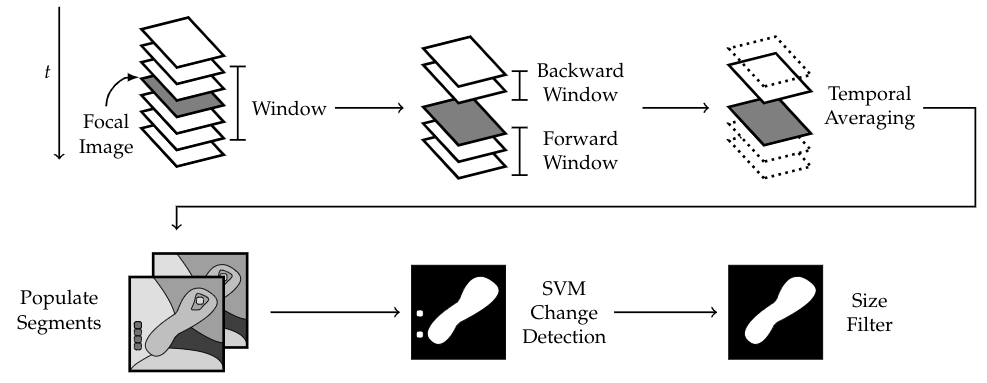
2. Methodology
2.1. Preprocessing Our Image Stack
2.2. Change Detection
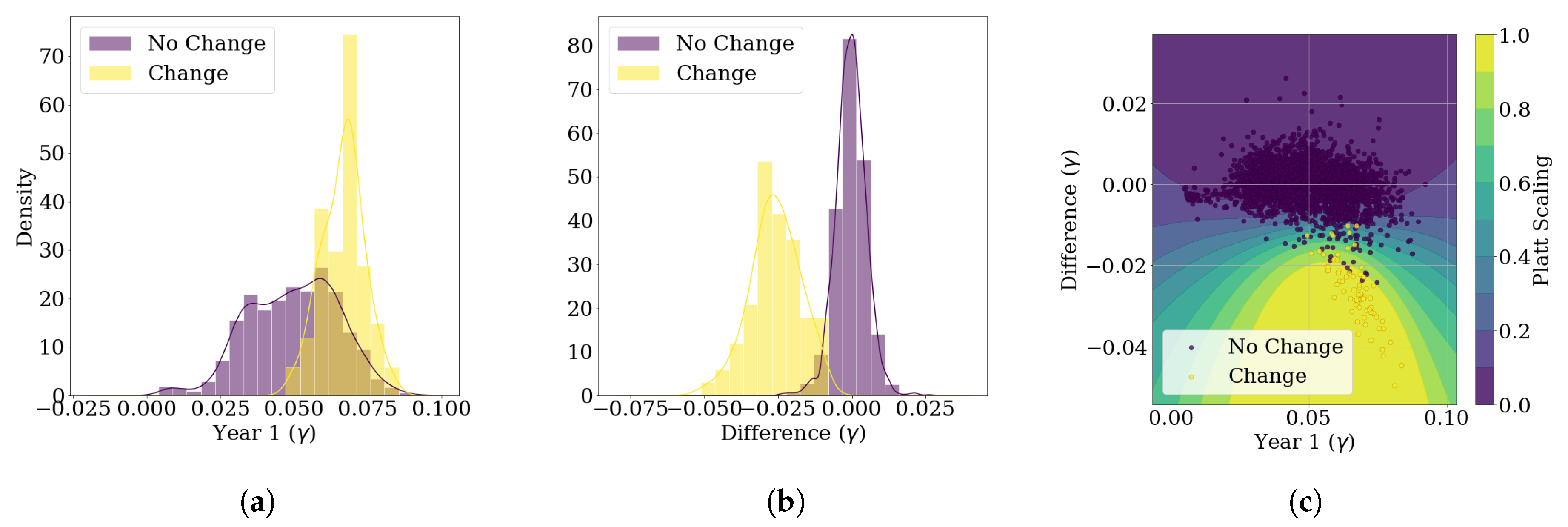
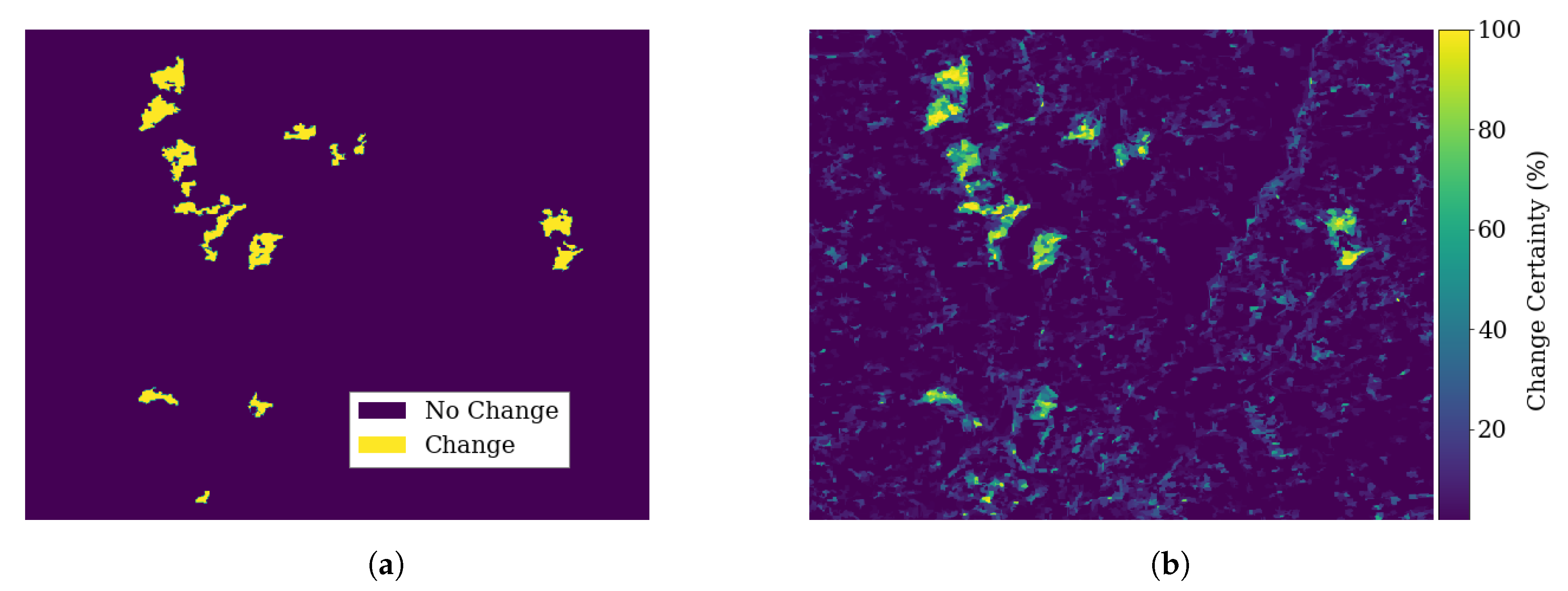
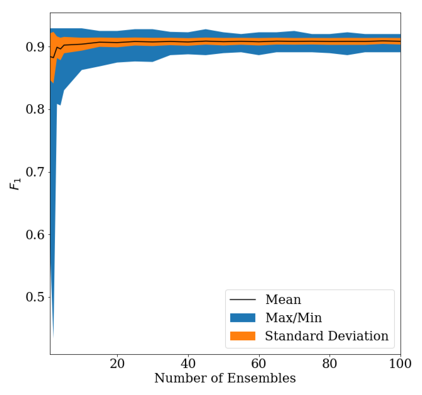
2.3. Empirical Uncertainty Measures
3. Applications
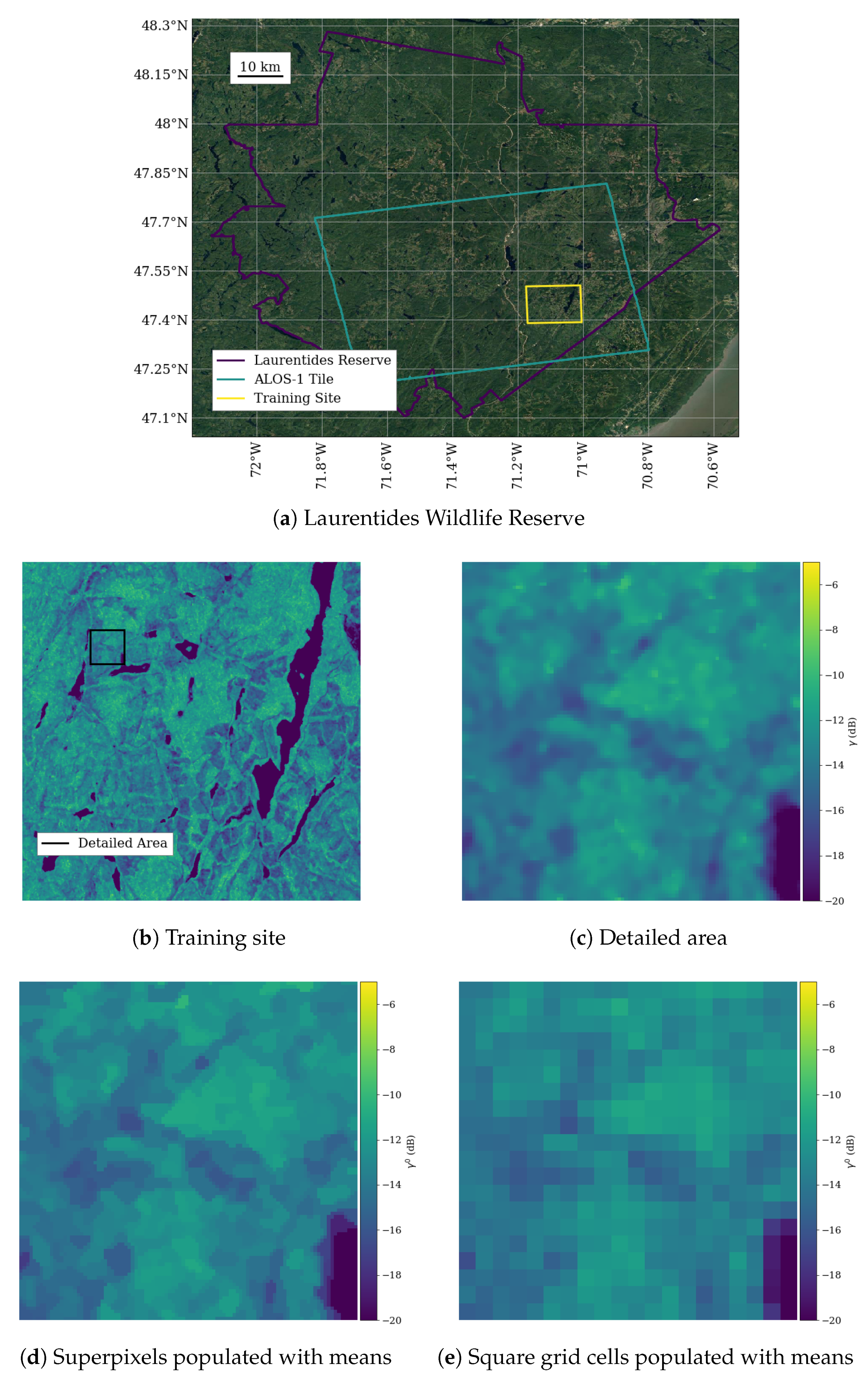
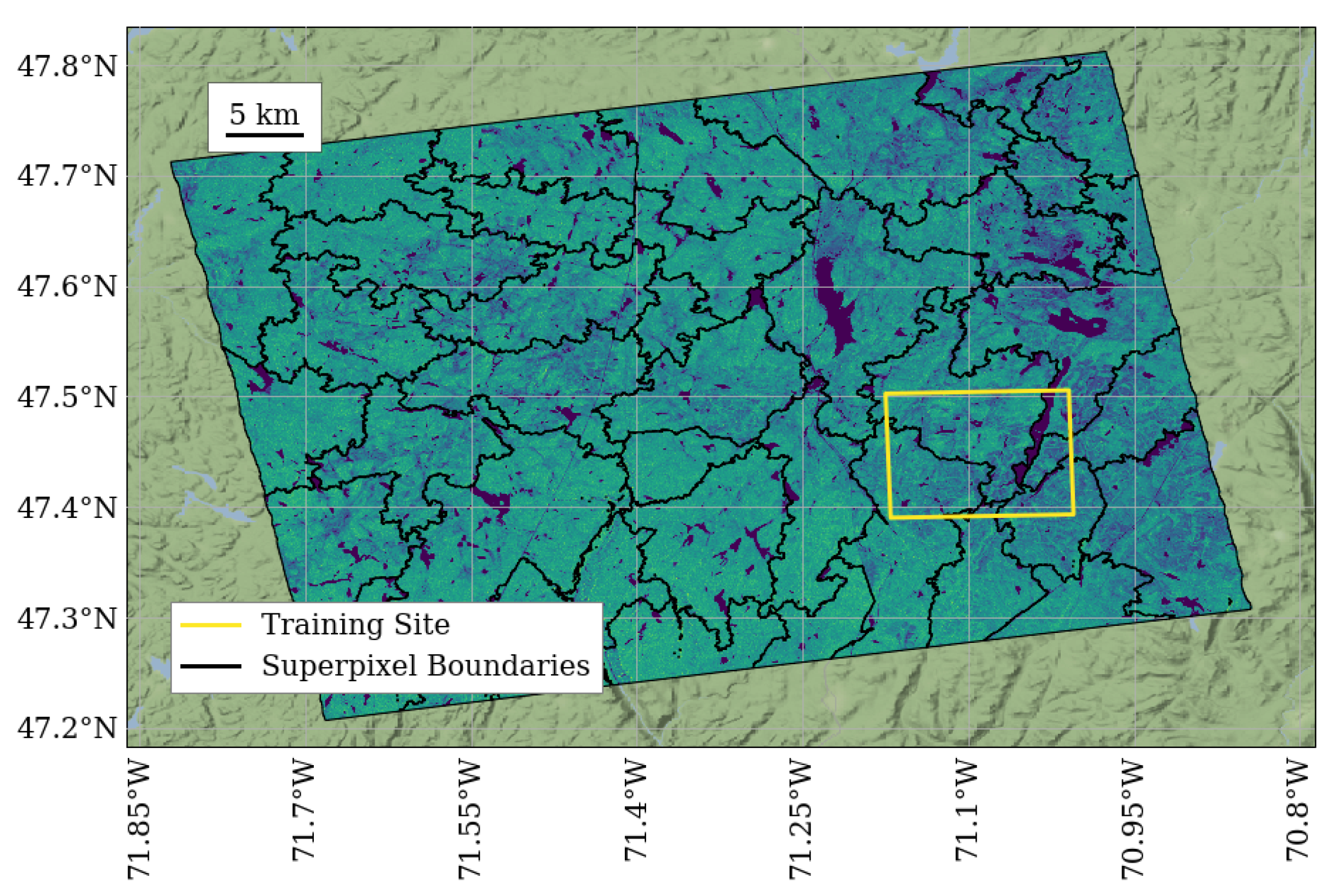
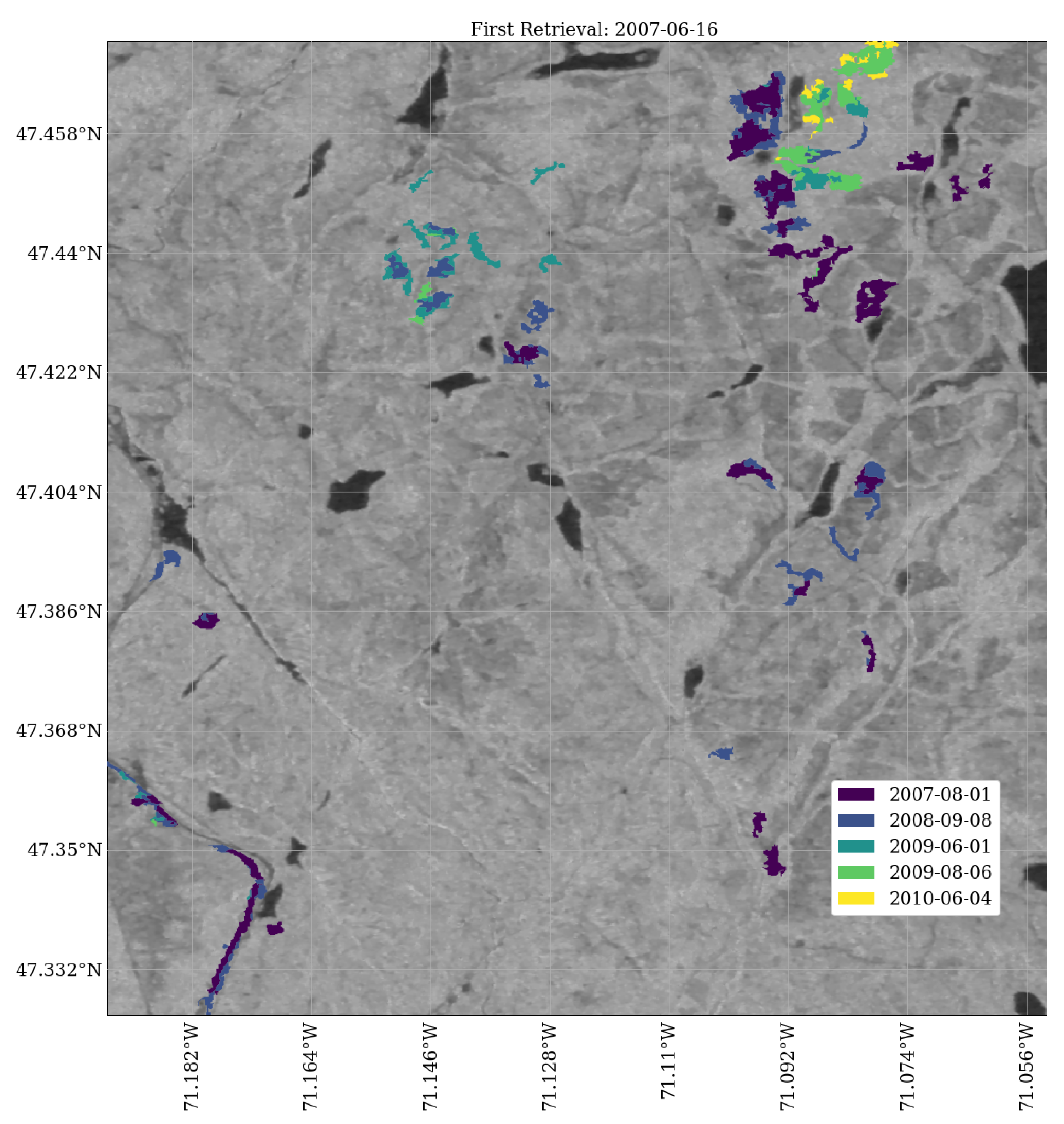
3.1. ALOS-1
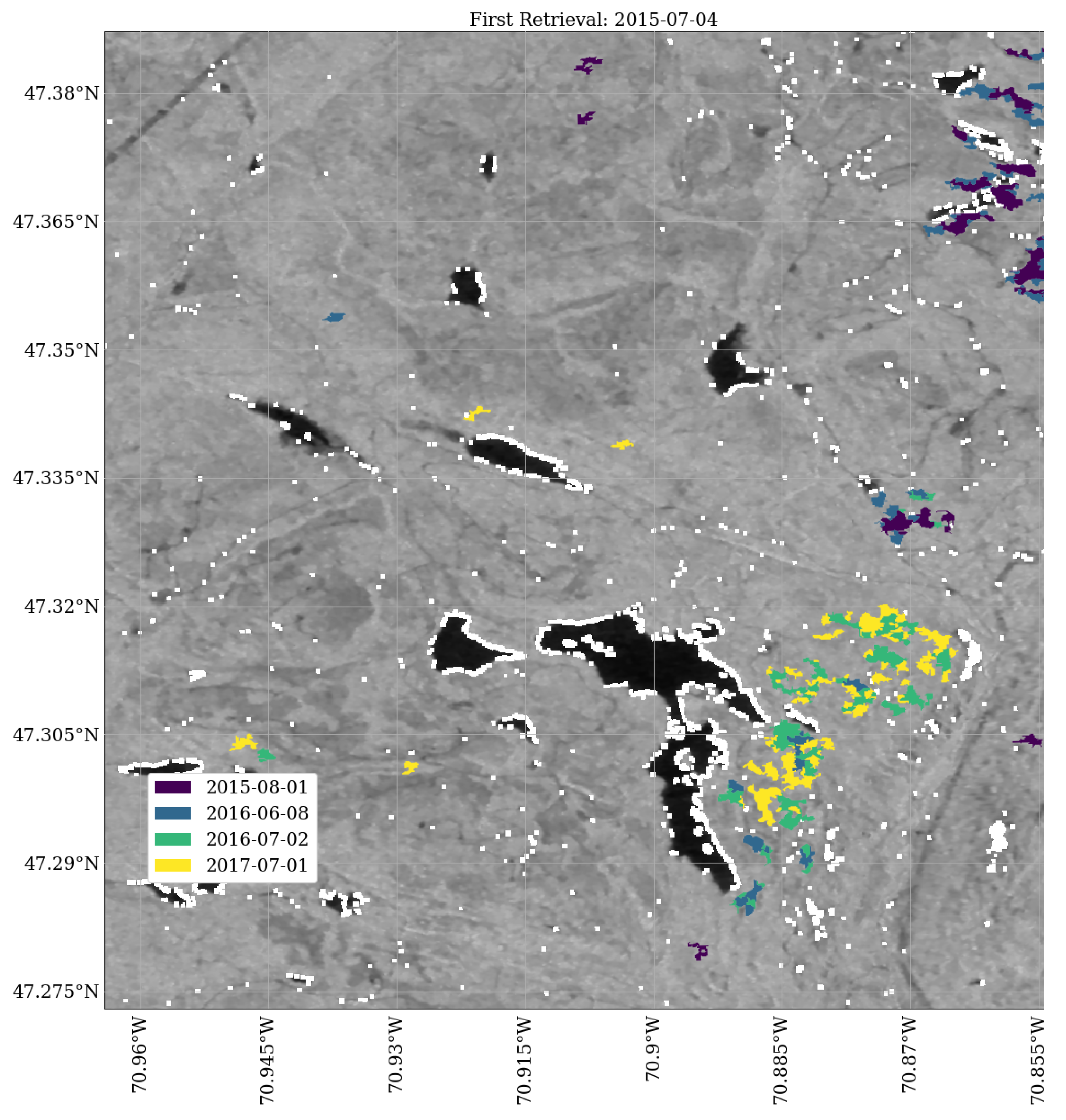
3.2. ALOS-2
4. Conclusions
Author Contributions
Funding
Acknowledgments
Conflicts of Interest
Abbreviations
| ALOS-1/-2 | Advanced Land Observing Satellite-1/-2 |
| ASF | Alaska Satellite Facility |
| NISAR | NASA-ISRO Synthetic Aperture Radar |
| PALSAR | Phased Array type L-band Synthetic Aperture Radar |
| RTC | Radiometrically and Terrain Corrected |
| SAOCOM | Satellites for Observation and Communications |
| SAR | Synthetic Aperture Radar |
| SVM | Support Vector Machine |
| TV Denoising | Total Variation Denoising |
Appendix A. Ensembling Support Vector Machines for Identifying Forest Loss

References
- Shimada, M.; Itoh, T.; Motooka, T.; Watanabe, M.; Shiraishi, T.; Thapa, R.; Lucas, R. New global Forest/Non-Forest Maps from ALOS PALSAR Data (2007–2010). Remote Sens. Environ. 2014, 155, 13–31. [Google Scholar] [CrossRef]
- NISAR Science Team. NASA-ISRO SAR Mission Science Users Handbook. 2019. Available online: https://nisar.jpl.nasa.gov/files/nisar/NISAR_Science_Users_Handbook.pdf (accessed on 14 January 2019).
- Chambers, J.Q.; Asner, G.P.; Morton, D.C.; Anderson, L.O.; Saatchi, S.S.; Espírito-Santo, F.D.; Palace, M.; Souza, C., Jr. Regional Ecosystem Structure and Function: Ecological Insights from Remote Sensing of Tropical Forests. Trends Ecol. Evol. 2007, 22, 414–423. [Google Scholar] [CrossRef] [PubMed]
- Avtar, R.; Sawada, H.; Takeuchi, W.; Singh, G. Characterization of Forests and Deforestation in Cambodia using ALOS/PALSAR Observation. Geocarto Int. 2012, 27, 119–137. [Google Scholar] [CrossRef]
- Thomas, N.; Lucas, R.; Bunting, P.; Hardy, A.; Rosenqvist, A.; Simard, M. Distribution and Drivers of Global Mangrove Forest Change, 1996–2010. PLoS ONE 2017, 12, e0179302. [Google Scholar] [CrossRef] [PubMed]
- Ren, X.; Malik, J. Learning a Classification Model for Segmentation. In Proceedings of the Ninth IEEE International Conference on Computer Vision, Nice, France, 13–16 October 2003; pp. 10–17. [Google Scholar]
- Flanders, D.; Hall-Beyer, M.; Pereverzoff, J. Preliminary Evaluation of eCognition Object-based Software for Cut Block Delineation and Feature Extraction. Can. J. Remote Sens. 2003, 29, 441–452. [Google Scholar] [CrossRef]
- Meinel, G.; Neubert, M. A Comparison of Segmentation Programs for High Resolution Remote Sensing Data. Int. Arch. Photogramm. Remote Sens. 2004, 35, 1097–1105. [Google Scholar]
- Felzenszwalb, P.F.; Huttenlocher, D.P. Efficient Graph-based Image Segmentation. Int. J. Comput. Vis. 2004, 59, 167–181. [Google Scholar] [CrossRef]
- Achanta, R.; Shaji, A.; Smith, K.; Lucchi, A.; Fua, P.; Süsstrunk, S. SLIC Superpixels Compared to State-of-the-Art Superpixel Methods. IEEE Trans. Pattern Anal. Mach. Intell. 2012, 34, 2274–2282. [Google Scholar] [CrossRef] [PubMed] [Green Version]
- Comaniciu, D.; Meer, P. Mean Shift: A Robust Approach toward Feature Space Analysis. IEEE Trans. Pattern Anal. Mach. Intell. 2002, 603–619. [Google Scholar] [CrossRef]
- Van der Walt, S.; Schönberger, J.L.; Nunez-Iglesias, J.; Boulogne, F.; Warner, J.D.; Yager, N.; Gouillart, E.; Yu, T. Scikit-image: Image Processing in Python. PeerJ 2014, 2, e453. [Google Scholar] [CrossRef] [PubMed]
- Lv, N.; Chen, C.; Qiu, T.; Sangaiah, A.K. Deep Learning and Superpixel Feature Extraction based on Contractive Autoencoder for Change Detection in SAR Images. IEEE Trans. Ind. Inform. 2018, 14, 5530–5538. [Google Scholar] [CrossRef]
- Gong, M.; Zhan, T.; Zhang, P.; Miao, Q. Superpixel-Based Difference Representation Learning for Change Detection in Multispectral Remote Sensing Images. IEEE Trans. Geosci. Remote Sens. 2017, 55, 2658–2673. [Google Scholar] [CrossRef]
- Zhou, L.; Cao, G.; Li, Y.; Shang, Y. Change Detection Based on Conditional Random Field with Region Connection Constraints in High-Resolution Remote Sensing Images. IEEE J. Sel. Top. Appl. Earth Obs. Remote Sens. 2016, 9, 3478–3488. [Google Scholar] [CrossRef]
- Huang, X.; Yang, W.; Xia, G.; Liao, M. Superpixel-based Change Detection in High Resolution SAR Images using Region Covariance Features. In Proceedings of the 8th International Workshop on the Analysis of Multitemporal Remote Sensing Images, Annecy, France, 22–24 July 2015; pp. 1–4. [Google Scholar]
- Ertürk, A.; Ertürk, S.; Plaza, A. Unmixing with SLIC Superpixels for Hyperspectral Change Detection. In Proceedings of the 2016 IEEE International Geoscience and Remote Sensing Symposium, Beijing, China, 10–15 July 2016; pp. 3370–3373. [Google Scholar]
- Clewley, D.; Bunting, P.; Shepherd, J.; Gillingham, S.; Flood, N.; Dymond, J.; Lucas, R.; Armston, J.; Moghaddam, M. A Python-based Open Source System for Geographic Object-based Image Analysis (GEOBIA) Utilizing Raster Attribute Tables. Remote Sens. 2014, 6, 6111–6135. [Google Scholar] [CrossRef]
- Liu, B.; Hu, H.; Wang, H.; Wang, K.; Liu, X.; Yu, W. Superpixel-based Classification with an Adaptive Number of Classes for Polarimetric SAR Images. IEEE Trans. Geosci. Remote Sens. 2013, 51, 907–924. [Google Scholar] [CrossRef]
- Thompson, D.R.; Mandrake, L.; Gilmore, M.S.; Castano, R. Superpixel Endmember Detection. IEEE Trans. Geosci. Remote Sens. 2010, 48, 4023–4033. [Google Scholar] [CrossRef]
- Zhang, S.; Li, S.; Fu, W.; Fang, L. Multiscale Superpixel-based Sparse Representation for Hyperspectral Image Classification. Remote Sens. 2017, 9, 139. [Google Scholar] [CrossRef]
- Audebert, N.; Saux, B.L.; Lefevre, S. How Useful is Region-based Classification of Remote Sensing Images in a Deep Learning Framework? arXiv, 2016; arXiv:1609.06861. [Google Scholar]
- Fan, F.; Ma, Y.; Li, C.; Mei, X.; Huang, J.; Ma, J. Hyperspectral Image Denoising with Superpixel Segmentation and Low-rank Representation. Inf. Sci. 2017, 397, 48–68. [Google Scholar] [CrossRef]
- Liu, X.; Jia, H.; Cao, L.; Wang, C.; Li, J.; Cheng, M. Superpixel-based Coastline Extraction in SAR Images with Speckle Noise Removal. In Proceedings of the IEEE International Geoscience and Remote Sensing Symposium, Beijing, China, 10–15 July 2016; pp. 1034–1037. [Google Scholar]
- Dupuy, S.; Herbreteau, V.; Feyfant, T.; Morand, S.; Tran, A. Land-cover Dynamics in Southeast Asia: Contribution of Object-oriented techniques for Change Detection. In Proceedings of the 4th International Conference on GEographic Object-Based Image Analysis (GEOBIA 2012), Rio de Janeiro, Brazil, 7–9 May 2012. [Google Scholar]
- Dingle Robertson, L.; King, D.J. Comparison of Pixel and Object-based Classification in Land Cover Change Mapping. Int. J. Remote Sens. 2011, 32, 1505–1529. [Google Scholar] [CrossRef]
- Myint, S.W.; Giri, C.P.; Wang, L.; Zhu, Z.; Gillette, S.C. Identifying Mangrove Species and Their Surrounding Land Use and Land Cover Classes using an Object-Oriented Approach with a Lacunarity Spatial Measure. GISci. Remote Sens. 2008, 45, 188–208. [Google Scholar] [CrossRef]
- Thomas, N.; Bunting, P.; Lucas, R.; Hardy, A.; Rosenqvist, A.; Fatoyinbo, T. Mapping Mangrove Extent and Change: A Globally Applicable Approach. Remote Sens. 2018, 10, 1466. [Google Scholar] [CrossRef]
- Kamal, M.; Phinn, S. Hyperspectral Data for Mangrove Species Mapping: A Comparison of Pixel-based and Object-based Approach. Remote Sens. 2011, 3, 2222–2242. [Google Scholar] [CrossRef]
- Small, D. Flattening Gamma: Radiometric Terrain Correction for SAR Imagery. IEEE Trans. Geosci. Remote Sens. 2011, 49, 3081–3093. [Google Scholar] [CrossRef]
- Celik, T. Unsupervised Change Detection in Satellite Images using Principal Component Analysis and k-means Clustering. IEEE Geosci. Remote Sens. Lett. 2009, 6, 772–776. [Google Scholar] [CrossRef]
- Nielsen, A.A. The Regularized Iteratively Reweighted MAD Method for Change Detection in Multi- and Hyper-Spectral Data. IEEE Trans. Image Process. 2007, 16, 463–478. [Google Scholar] [CrossRef] [PubMed]
- Li, S.; Jia, X.; Zhang, B. Superpixel-based Markov Random Field for Classification of Hyperspectral Images. In Proceedings of the IEEE International Geoscience and Remote Sensing Symposium-IGARSS, Melbourne, Australia, 21–26 July 2013; pp. 3491–3494. [Google Scholar]
- Bruzzone, L.; Prieto, D.F. Automatic Analysis of the Difference Image for Unsupervised Change Detection. IEEE Trans. Geosci. Remote Sens. 2000, 38, 1171–1182. [Google Scholar] [CrossRef]
- Hansen, M.C.; Potapov, P.V.; Moore, R.; Hancher, M.; Turubanova, S.A.A.; Tyukavina, A.; Thau, D.; Stehman, S.V.; Goetz, S.J.; Loveland, T.R.; et al. High-resolution Global Maps of 21st Century Forest Cover Change. Science 2013, 342, 850–853. [Google Scholar] [CrossRef] [PubMed]
- Zhu, X.X.; Tuia, D.; Mou, L.; Xia, G.S.; Zhang, L.; Xu, F.; Fraundorfer, F. Deep Learning in Remote Sensing: A Comprehensive Review and List of Resources. IEEE Geosci. Remote Sens. Mag. 2017, 5, 8–36. [Google Scholar] [CrossRef] [Green Version]
- Zhang, L.; Zhang, L.; Du, B. Deep Learning for Remote Sensing Data: A Technical Tutorial on the State of the Art. IEEE Geosci. Remote Sens. Mag. 2016, 4, 22–40. [Google Scholar] [CrossRef]
- Ministry of Forests, Wildlife and Parks. EcoforestMap with Distrubances. 2018. Quebec Data Portal. Available online: https://www.donneesquebec.ca/recherche/fr/dataset/carte-ecoforestiere-avec-perturbations (accessed on 14 January 2019).
- Mou, L.; Bruzzone, L.; Zhu, X.X. Learning Spectral-Spatial-Temporal features via a Recurrent Convolutional Neural Network for Change Detection in Multispectral Imagery. IEEE Trans. Geosci. Remote Sens. 2019, 57, 924–935. [Google Scholar] [CrossRef]
- Audebert, N.; Le Saux, B.; Lefèvre, S. Semantic Segmentation of Earth Observation Data using Multimodal and Multi-Scale Deep Networks. In Proceedings of the Asian Conference on Computer Vision, Taipei, Taiwan, 20–24 November 2016; pp. 180–196. [Google Scholar]
- Lyu, H.; Lu, H.; Mou, L. Learning a Transferable Change Rule from a Recurrent Neural Network for Land Cover Change Detection. Remote Sens. 2016, 8, 506. [Google Scholar] [CrossRef]
- Alaska Satellite Facility. ASF DAAC 2015; Includes Material©JAXA/METI 2007. Available online: http://dx.doi.org/10.5067/Z97HFCNKR6VA (accessed on 14 January 2019).
- Simard, M.; Riel, B.V.; Denbina, M.; Hensley, S. Radiometric Correction of Airborne Radar Images over Forested Terrain with Topography. IEEE Trans. Geosci. Remote Sens. 2016, 54, 4488–4500. [Google Scholar] [CrossRef]
- Rudin, L.I.; Osher, S.; Fatemi, E. Nonlinear Total Variation Based Noise Removal Algorithms. Phys. D Nonlinear Phenom. 1992, 60, 259–268. [Google Scholar] [CrossRef]
- Bioucas-Dias, J.M.; Figueiredo, M.A.T. Multiplicative Noise Removal Using Variable Splitting and Constrained Optimization. IEEE Trans. Image Process. 2010, 19, 1720–1730. [Google Scholar] [CrossRef] [PubMed] [Green Version]
- Zhao, Y.; Liu, J.G.; Zhang, B.; Hong, W.; Wu, Y.R. Adaptive Total Variation Regularization based SAR Image Despeckling and Despeckling Evaluation Index. IEEE Trans. Geosci. Remote Sens. 2015, 53, 2765–2774. [Google Scholar] [CrossRef]
- Martinis, S.; Kuenzer, C.; Wendleder, A.; Huth, J.; Twele, A.; Roth, A.; Dech, S. Comparing Four Operational SAR-based Water and Flood Detection Approaches. Int. J. Remote Sens. 2015, 36, 3519–3543. [Google Scholar] [CrossRef]
- Wang, M.; Liu, X.; Gao, Y.; Ma, X.; Soomro, N.Q. Superpixel Segmentation: A Benchmark. Signal Process. Image Commun. 2017, 56, 28–39. [Google Scholar] [CrossRef]
- Stutz, D.; Hermans, A.; Leibe, B. Superpixels: An Evaluation of the State-of-the-Art. Comput. Vis. Image Underst. 2018, 166, 1–27. [Google Scholar] [CrossRef]
- Boser, B.E.; Guyon, I.M.; Vapnik, V.N. A Training Algorithm for Optimal Margin Classifiers. In Proceedings of the 5th Annual Workshop on Computational Learning Theory, Pittsburgh, PA, USA, 27–29 July 1992; pp. 144–152. [Google Scholar]
- Platt, J. Probabilistic Outputs for Support Vector Machines and Comparisons to Regularized Likelihood Methods. Adv. Large Margin Classif. 1999, 10, 61–74. [Google Scholar]
- Quebec Transportation. Route 73/175 Project. 2008. Available online: https://web.archive.org/web/20110716214657/http://www.mtq.gouv.qc.ca/portal/page/portal/grands_projets/trouver_grand_projet/axe_routier_73_175 (accessed on 14 December 2018).
- JAXA. ALOS/ALOS-2 User Interface Gateway. Available online: https://auig2.jaxa.jp/ips/home (accessed on 14 December 2018).
- Murphy, K.P. Machine Learning: A Probabilistic Perspective; MIT Press: Cambridge, MA, USA, 2012. [Google Scholar]


| Sensor | Mode | Available Dates Italicized Are Used in Time Series and Underlined Are Used for SVM Training and Validation | Resolution (m) | Elevation /max (m) | Slope / + (degrees) | Total Area (ha) |
|---|---|---|---|---|---|---|
| ALOS-1 | Fine Beam Dual | 2007-06-16, 2007-08-01, 2008-09-18, 2009-06-21, 2009-08-06, 2010-06-24, 2010-08-09, 2010-09-24 | 12.5 | 801/1148 | 8.44/28.13 | |
| ALOS-2 | Strip Map (10 meter) | 2014-11-22, 2014-12-20, 2015-02-28, 2015-07-04, 2015-08-01, 2016-06-18, 2016-07-02, 2016-11-19, 2017-07-01, 2017-12-16 | 10 | 796/1161 | 8.90/28.79 |
| Segments | (Training Site) | (Full Tile) | Producer Accuracy (Full Tile) | User Accuracy (Full Tile) |
|---|---|---|---|---|
| Quebec Segments | 0.922 | 0.7719 | 0.6871 | 0.8806 |
| Superpixels | 0.704 | 0.597 | 0.5377 | 0.6709 |
| Pixels | 0.722 | 0.571 | 0.5131 | 0.6436 |
| Squares | 0.708 | 0.567 | 0.5044 | 0.6473 |
| Segments | (Training Site) | (Full Tile) | Producer Accuracy (Full Tile) | User Accuracy (Full Tile) |
|---|---|---|---|---|
| Landsat Segments | 0.831 | 0.5169 | 0.5329 | 0.5019 |
| Superpixels | 0.712 | 0.4841 | 0.5098 | 0.4609 |
| Pixels | 0.716 | 0.4668 | 0.4672 | 0.4665 |
| Squares | 0.71 | 0.458 | 0.4371 | 0.481 |
© 2019 by the authors. Licensee MDPI, Basel, Switzerland. This article is an open access article distributed under the terms and conditions of the Creative Commons Attribution (CC BY) license (http://creativecommons.org/licenses/by/4.0/).
Share and Cite
Marshak, C.; Simard, M.; Denbina, M. Monitoring Forest Loss in ALOS/PALSAR Time-Series with Superpixels. Remote Sens. 2019, 11, 556. https://doi.org/10.3390/rs11050556
Marshak C, Simard M, Denbina M. Monitoring Forest Loss in ALOS/PALSAR Time-Series with Superpixels. Remote Sensing. 2019; 11(5):556. https://doi.org/10.3390/rs11050556
Chicago/Turabian StyleMarshak, Charlie, Marc Simard, and Michael Denbina. 2019. "Monitoring Forest Loss in ALOS/PALSAR Time-Series with Superpixels" Remote Sensing 11, no. 5: 556. https://doi.org/10.3390/rs11050556