Processing Thermal Infrared Imagery Time-Series from Volcano Permanent Ground-Based Monitoring Network. Latest Methodological Improvements to Characterize Surface Temperatures Behavior of Thermal Anomaly Areas


Abstract
:
1. Introduction
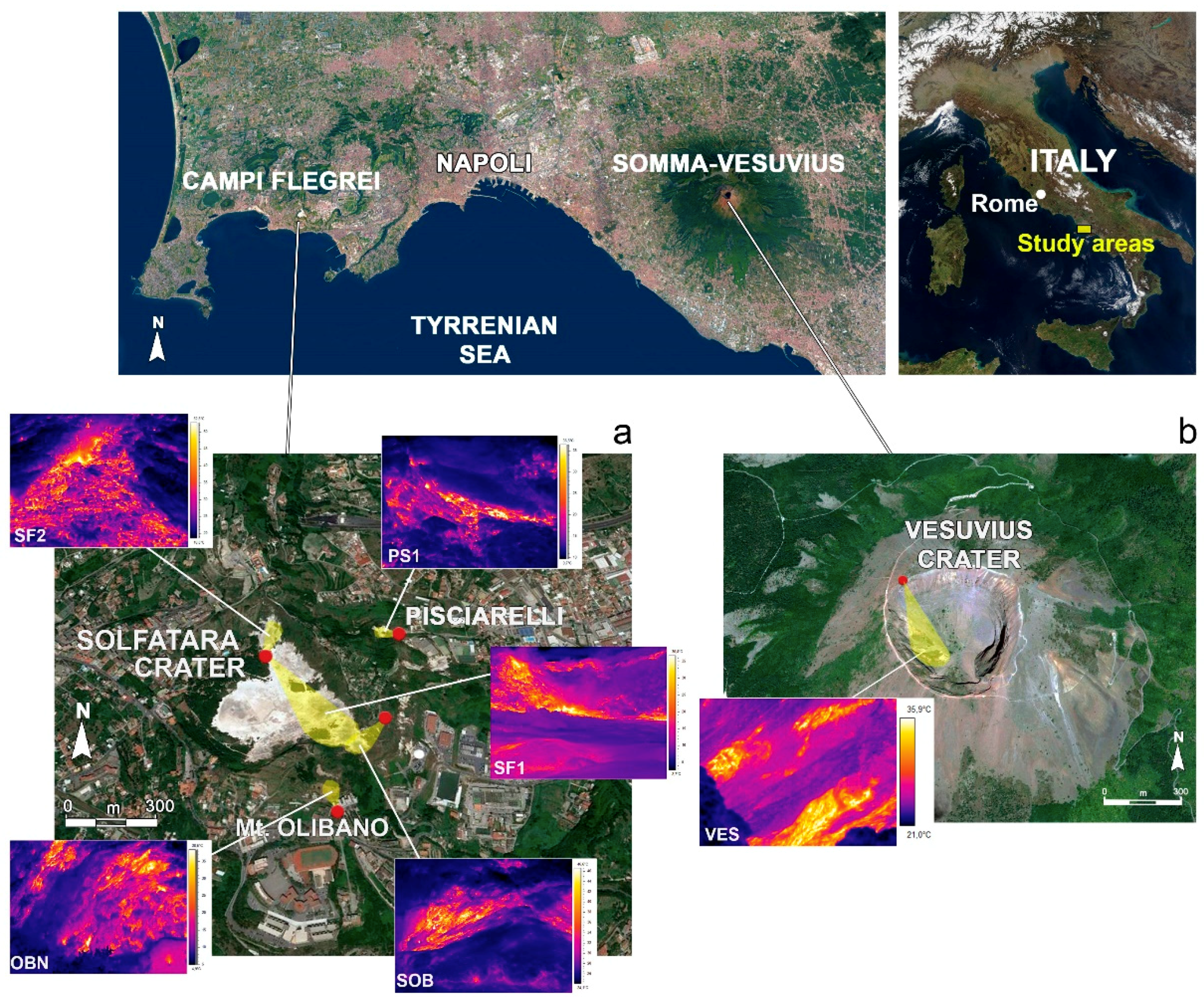
2. The Study Areas
3. Materials and Methods
3.1. The IR Sensors and Data Acquisition
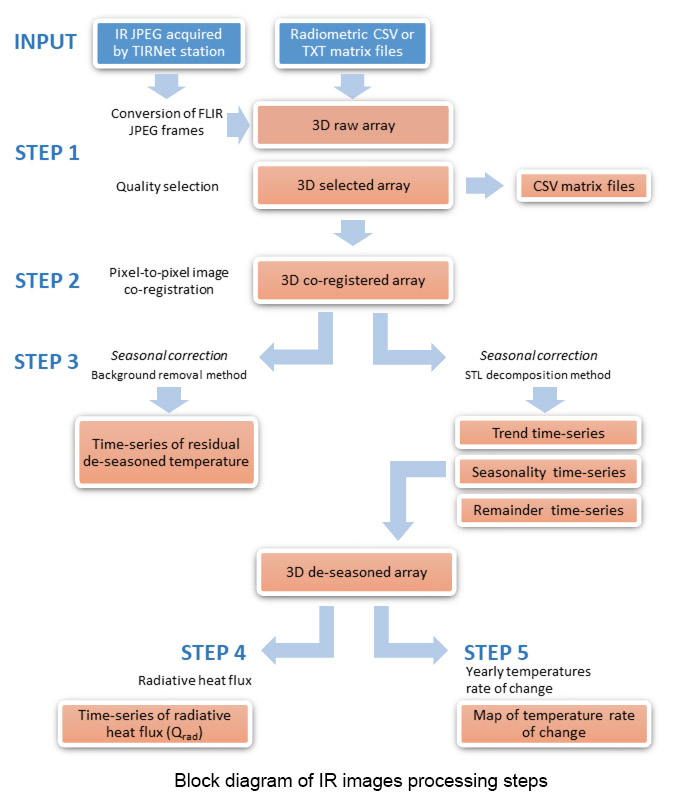
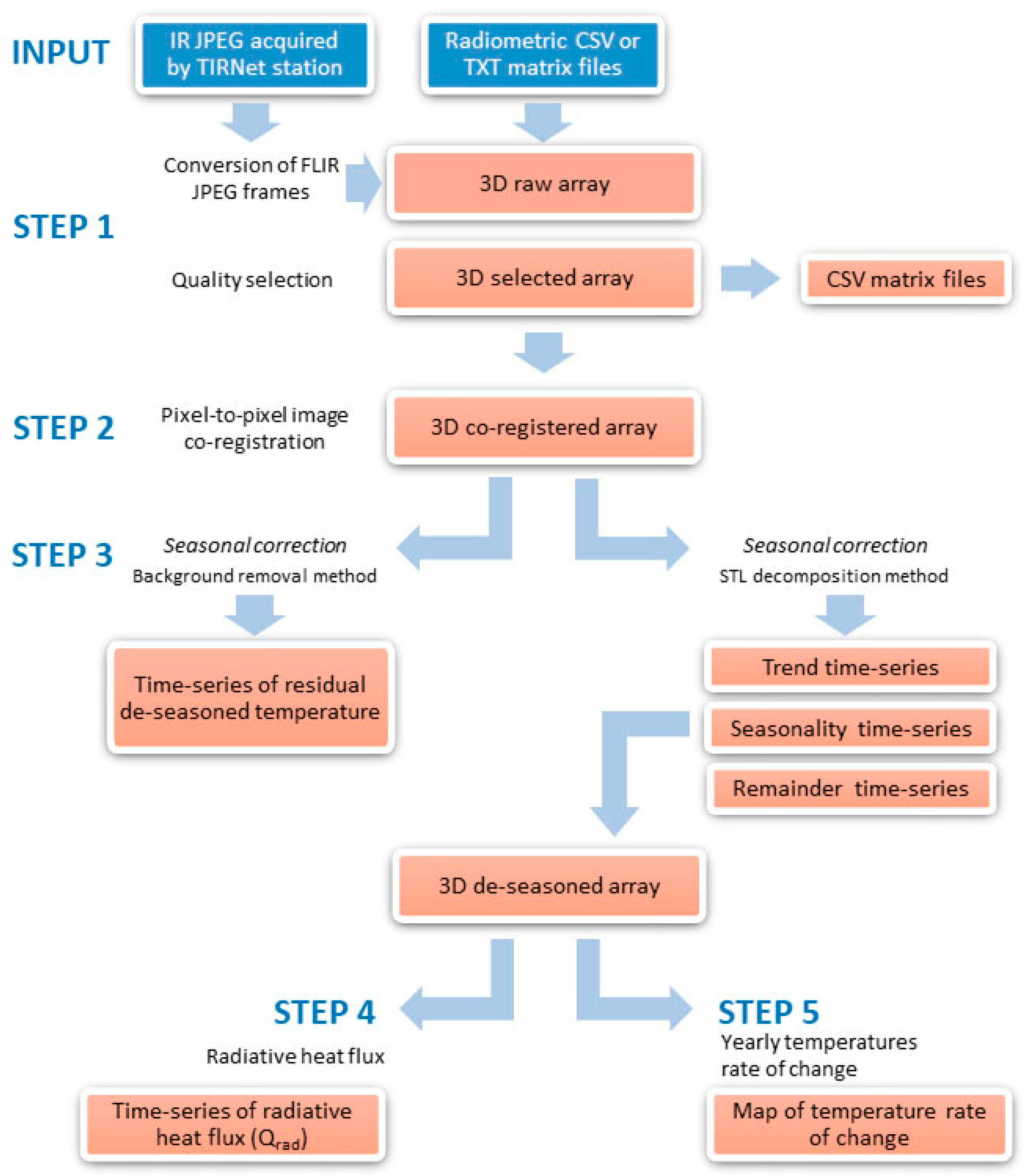
3.2. Data Processing Procedures
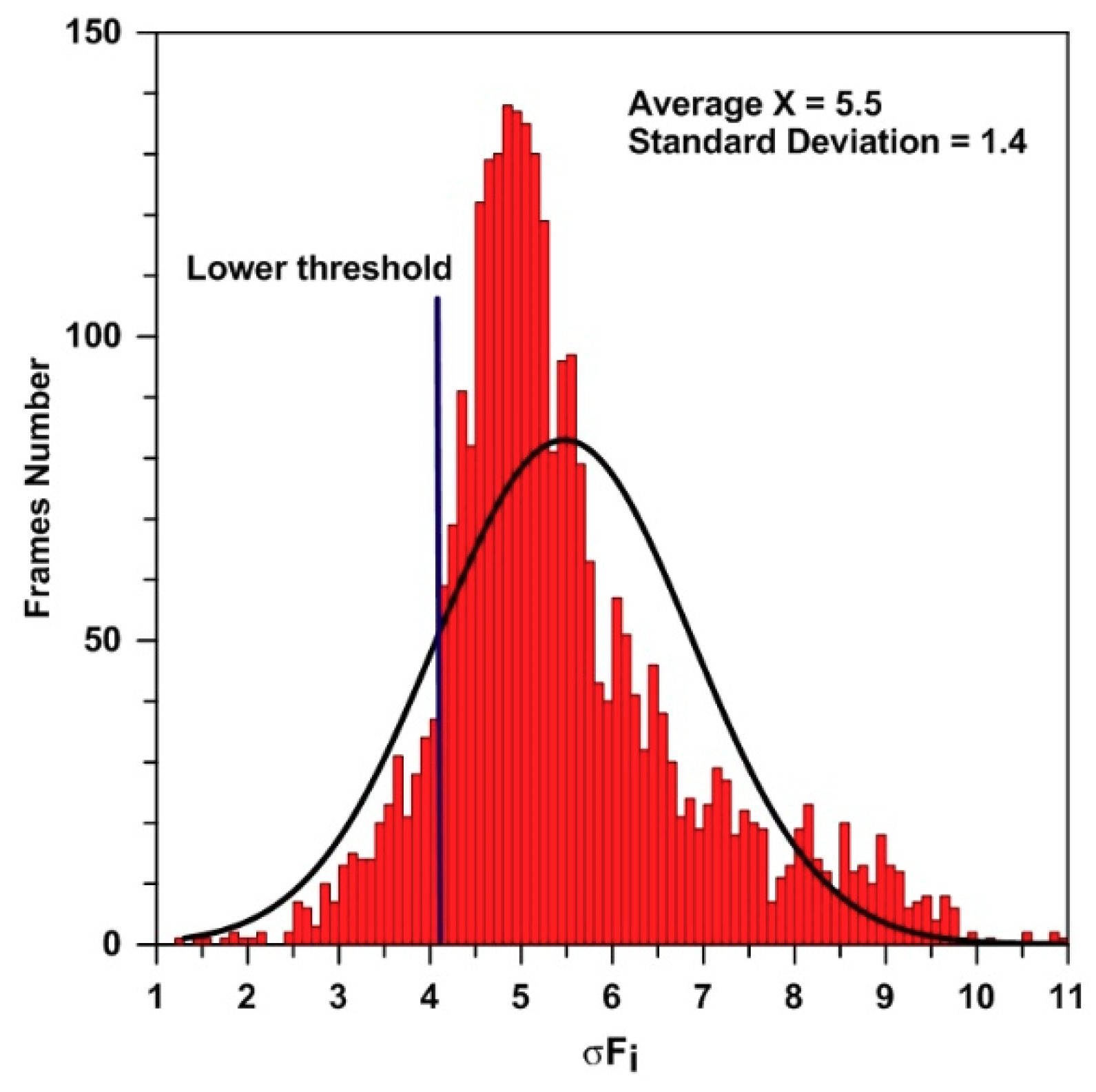
3.2.1. Step 1—IR Files Conversion, Archiving and Image Quality Selection
3.2.2. Step 2—IR Frames Co-registration
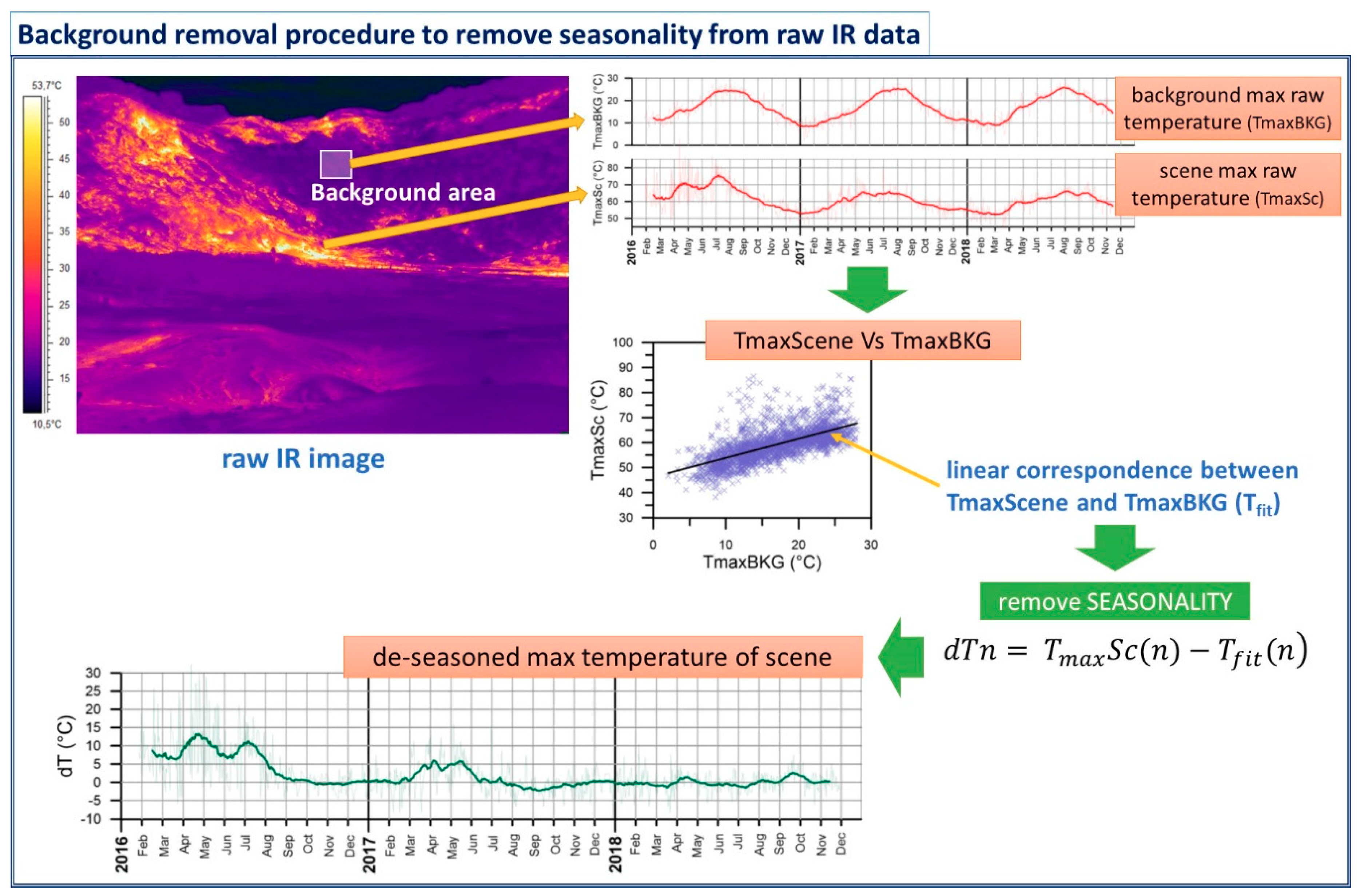
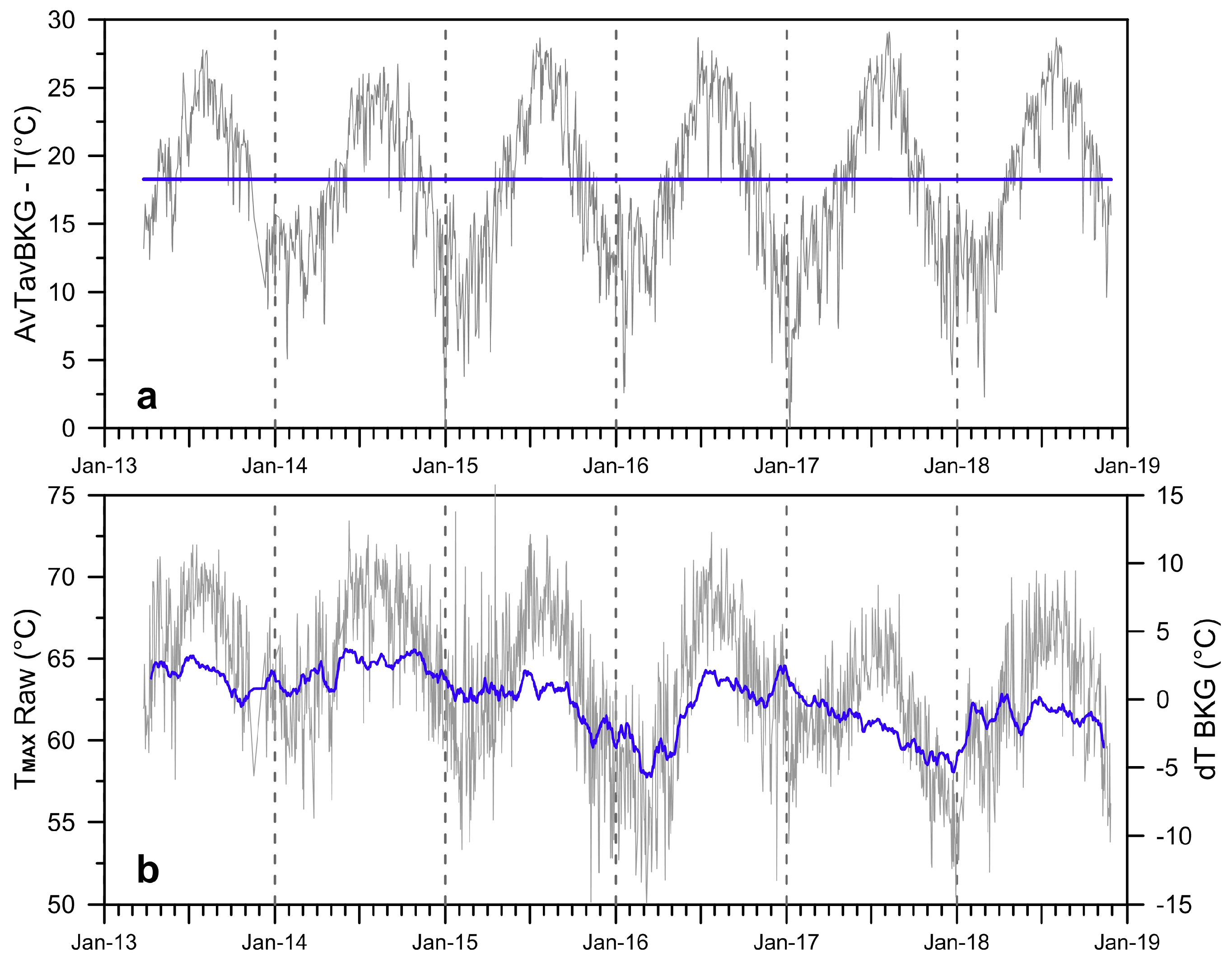
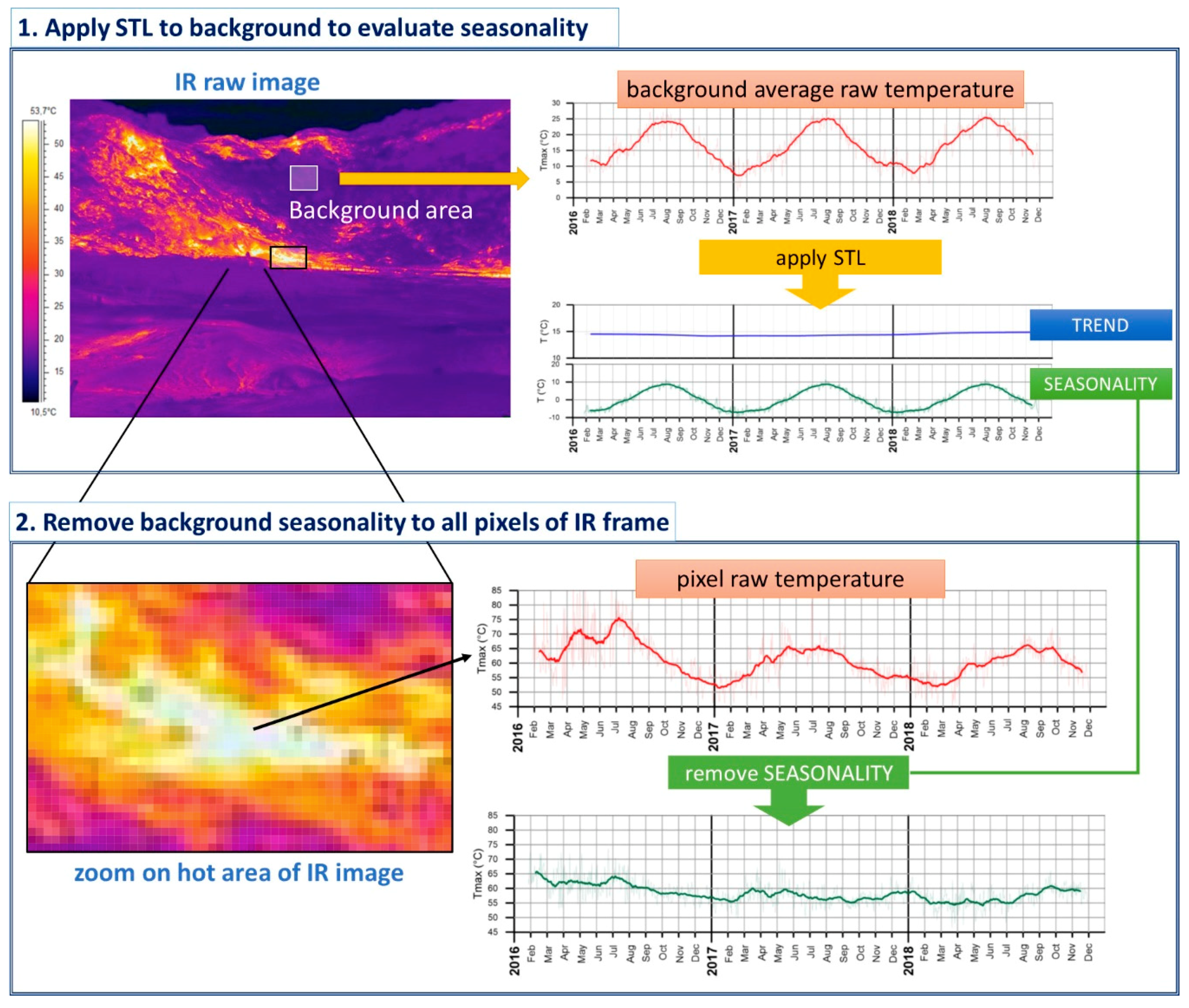
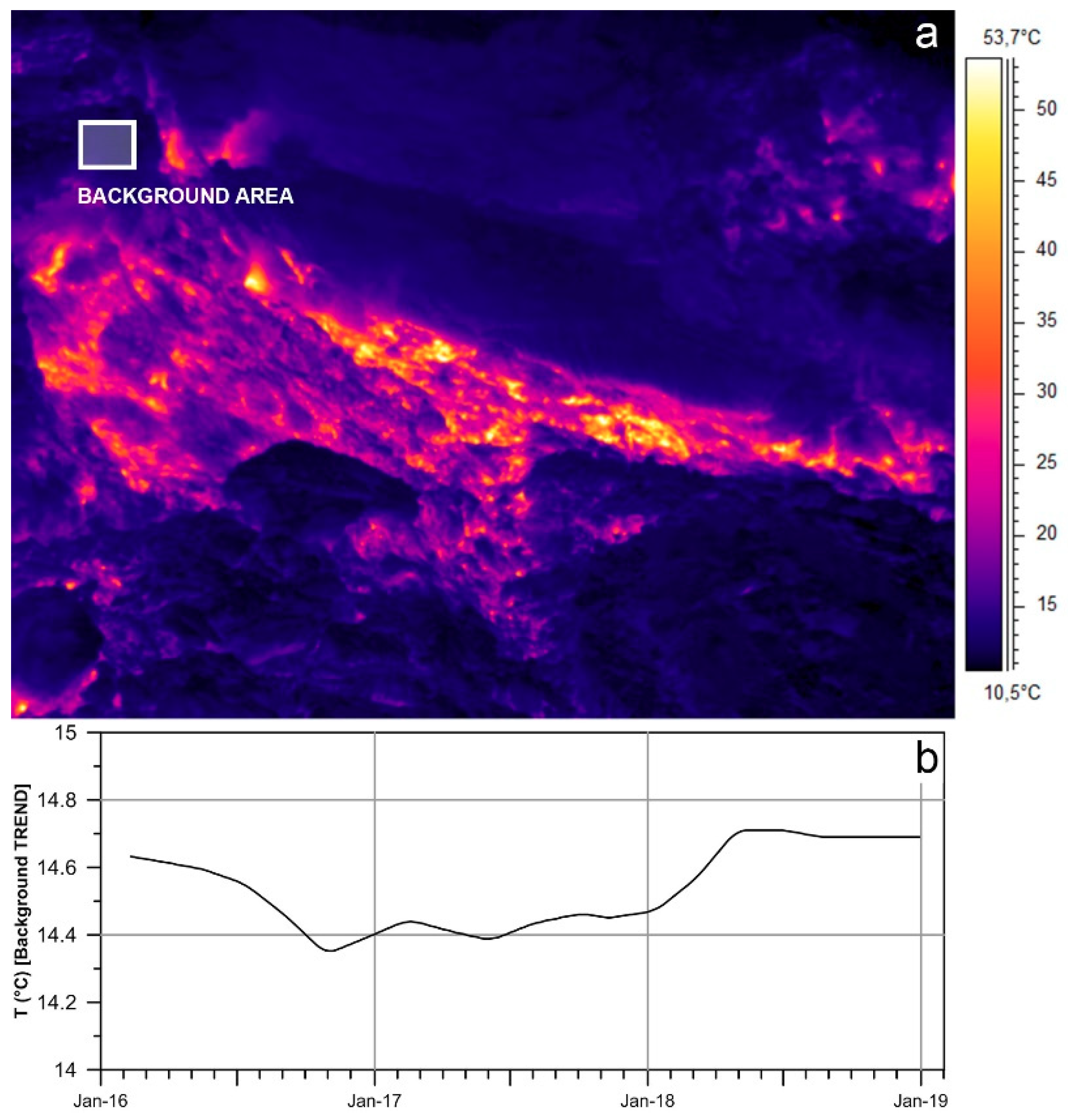
3.2.3. Step 3—Seasonal Component Removal
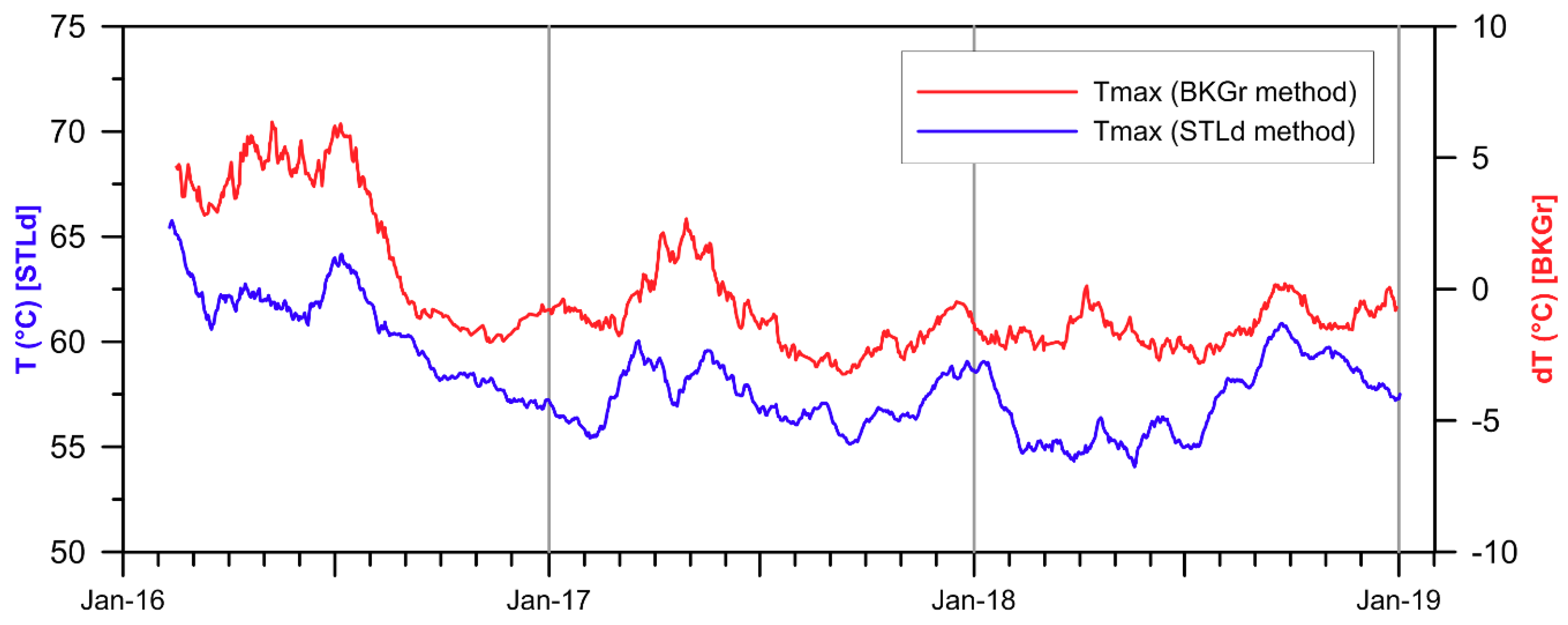
The Background Removal Procedure (BKGr)
The STL Decomposition Method (STLd)
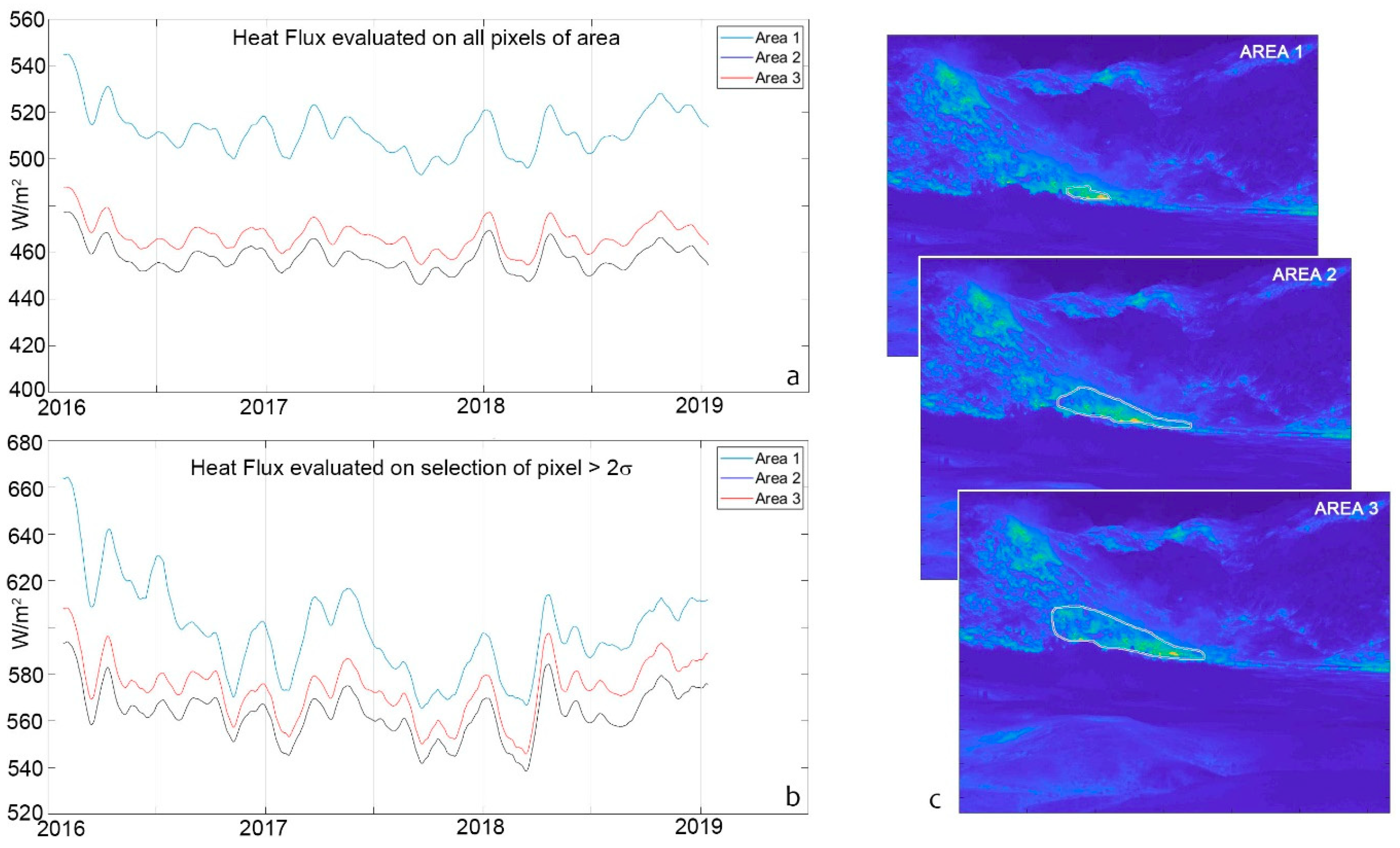
3.2.4. Step 4—Radiative Heat Flux (Qrad)
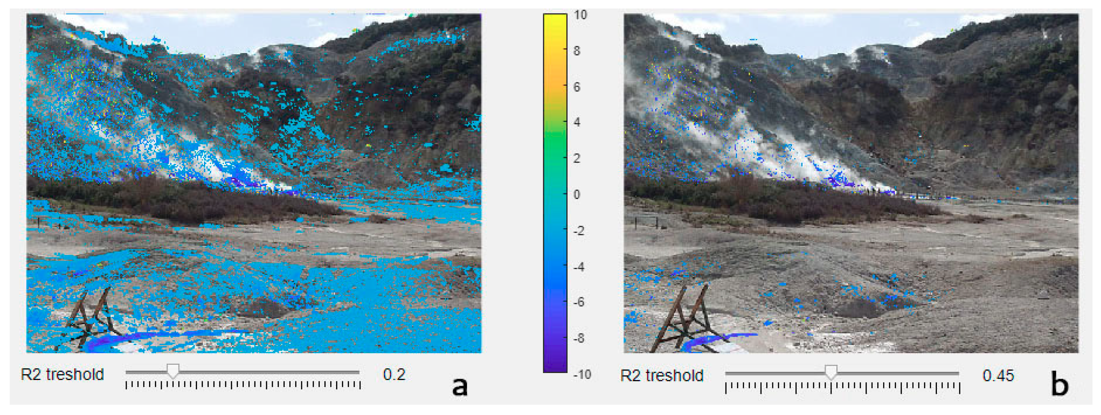
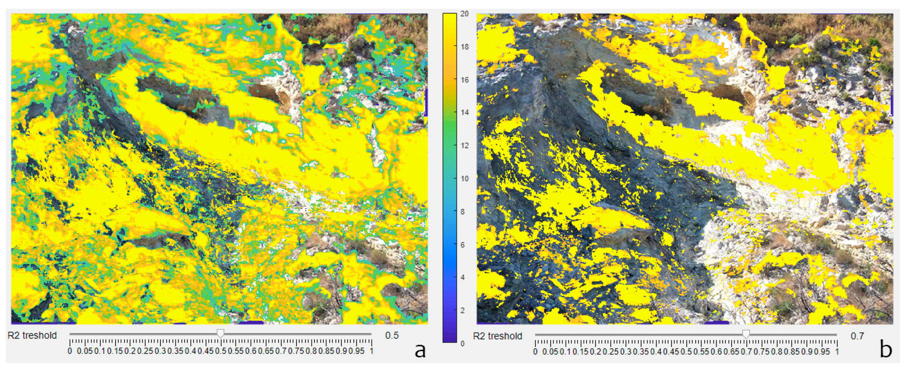
3.2.5. Step 5—Yearly Rate of Temperatures Change (YRTC)
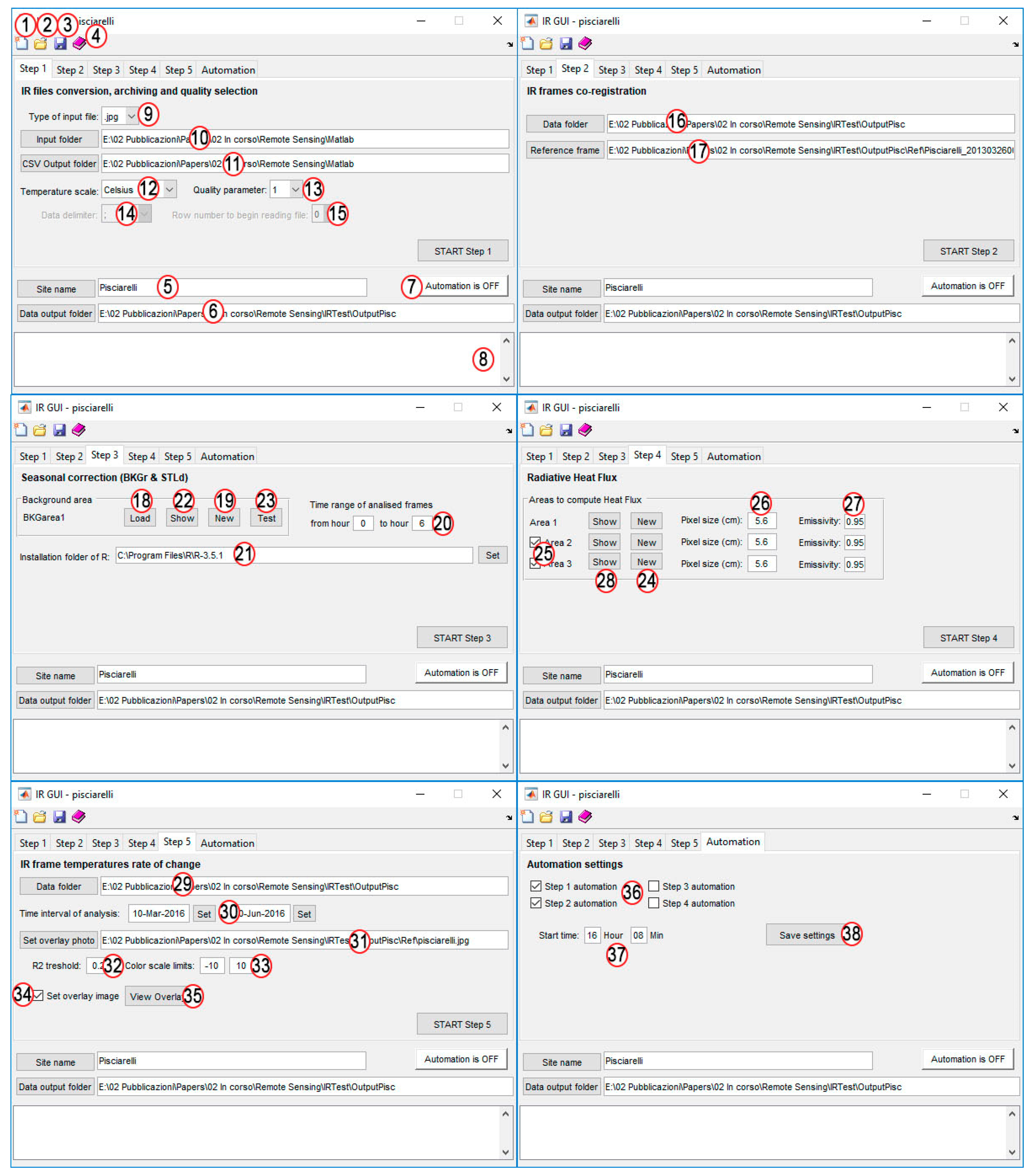
3.3. System Automation and Graphic Interface
4. Results and Discussion
4.1. Data Quality Selection
4.2. Seasonal Component Removal
4.3. Radiative Heat Flux Estimate
4.4. Yearly Rate of Temperature Change Estimate
5. Conclusions
Supplementary Materials
Author Contributions
Funding
Conflicts of Interest
Appendix A


| Script Name | ||
|---|---|---|
| asira_gui.m | ||
| Functionality | ||
| Graphic user interface (GUI) with management of configuration file | ||
| Inputs description | Inputs type | ID |
| New configuration file | File name in common dialog window by pressing toolbar button | 1 |
| Open configuration file | File name in common dialog window by pressing toolbar button | 2 |
| Save current configuration file | Toolbar button | 3 |
| Open Operative Guide | Toolbar button | 4 |
| Site name (study area) | String inserted by edit window | 5 |
| Output folder of processed data (common to all steps) | Folder path inserted by common dialog window | 6 |
| Automation button (activate/deactivate automation) | Button | 7 |
| Enable/disable automation of processing step | Check box selection | 36 |
| Time to start automation process | Text boxes to input Hour and Minutes | 37 |
| Save automation settings | Button | 38 |
| Outputs description | Output type | ID |
| Log window showing processing messages | Text displayed in box area | 8 |
| Script Name | ||
|---|---|---|
| step01.m | ||
| Functionality | ||
| IR files conversion, archiving and quality selection (tab ‘Step 1′ in GUI) | ||
| Inputs description | Inputs type | ID |
| Type of input file | ‘.jpg/.csv/.txt’ inserted by drop-down menu | 9 |
| Data input folder | Folder path in common dialog window by pressing button | 10 |
| Output folder of CSV files 1 | Folder path in common dialog window by pressing button | 11 |
| Temperature scale | ‘Celsius/Fahrenheit’ inserted by drop-down menu | 12 |
| Quality selection parameter | ‘05/1/1.5/2′ inserted by drop-down menu | 13 |
| Data delimiter of csv/txt input files 1 | ‘,/;/TAB/SPACE’ inserted by drop-down menu | 14 |
| Row number to begin reading data in csv/txt file | Integer inserted by drop-down menu | 15 |
| Outputs description | Output type | ID |
| Log window showing processing messages | Text displayed in box area | 8 |
| CSV files of quality selected IR frames | Matrix CSV files of temperature values from IR scenes | |
| Arrays of quality selected IR data, yearly split | Matlab (.mat) archives in output folder | |
| Script Name | ||
|---|---|---|
| step02.m | ||
| Functionality | ||
| IR frames co-registration (tab ‘Step 2′ in GUI) | ||
| Inputs description | Inputs type | ID |
| Data input folder (containing .mat archives of Step 1) | Folder path in common dialog window by pressing button | 16 |
| Reference IR frame | File name & path in common dialog window by pressing button | 17 |
| Outputs description | Output type | ID |
| Log window showing processing messages | Text displayed in box area | 8 |
| Arrays of co-registered IR data, yearly split | Matlab (.mat) archives in output folder | |
| Script Name | ||
|---|---|---|
| step03.m | ||
| Functionality | ||
| Seasonal correction with BKGr and STLd methods (tab ‘Step 3′ in GUI) | ||
| Inputs description | Inputs type | ID |
| Load background area | File name & path in common dialog window by pressing button | 18 |
| New background area | File name & path in common dialog window by pressing button and selection of area over IR image | 19 |
| Daily time range of IR frames | Integers (hours) in text boxes | 20 |
| Installation folder of R statistical package (STL) | Folder path in common dialog window by pressing button | 21 |
| Outputs description | Output type | ID |
| Log window showing processing messages | Text displayed in box area | 8 |
| Show background area image | JPEG image of background area | 22 |
| Test background area image | Plots of Tmax and STL Trend of background area (by choice) | 23 |
| Array of de-seasoned IR data | Matlab (.mat) archive in output folder | |
| Data sheets of processed temperatures of IR frames | Excel file in output folder | |
| Script Name | ||
|---|---|---|
| step04.m | ||
| Functionality | ||
| Radiative heat flux estimation (tab ‘Step 4′ in GUI) | ||
| Inputs description | Inputs type | ID |
| New heat flux areas (Area 1, 2, 3) | Selection of heat flux area over IR image by pressing button | 24 |
| Enable/disable heat flux areas to process (Area 2, 3) | Check box selection | 25 |
| Pixel size of heat flux areas (Area 1, 2, 3) | Numeric values in text box | 26 |
| Emissivity of heat flux areas (Area 1, 2, 3) | Numeric values in text box | 27 |
| Outputs description | Output type | ID |
| Log window showing processing messages | Text displayed in box area | 8 |
| Show heat flux areas (areas 1, 2, 3) | JPEG images by pressing button | 28 |
| Arrays of heat flux data | Matlab (.mat) archive in output folder | |
| Data sheets of heat fluxes of IR frames | Excel file in output folder | |
| Script Name | ||
|---|---|---|
| step05.m | ||
| Functionality | ||
| Temperature rate of change during selected time-period (tab ‘Step 5′ in GUI) | ||
| Inputs description | Inputs type | ID |
| Data input folder (containing .mat output files of previous Steps) | Folder path in common dialog window by pressing button | 29 |
| Time interval of analysis | Dates picked over calendar | 30 |
| Photo of studied area to use in data overlay | File name & path in common dialog window by pressing button | 31 |
| Threshold value of R2 extracted from linear regressions of pixels time-series | Numeric values in text box | 32 |
| Limits of color scale to use in temperature rate of change map | Numeric values in text box | 33 |
| Enable/disable data overlay on photo of studied area | Check box selection | 34 |
| Outputs description | Output type | ID |
| Log window showing processing messages | Text displayed in box area | 8 |
| Show map of temperature rate of change | JPEG image by pressing button | 35 |
| Arrays of temperature rate of change data | Matlab (.mat) archive in output folder | |
| Data sheets of temperature rate of change data | Excel file in output folder | |
References
- Ball, M.; Pinkerton, H. Factors affecting the accuracy of thermal imaging cameras in volcanology. J. Geophys. Res. 2006, 111, B11203. [Google Scholar] [CrossRef]
- Lagios, E.; Vassilopoulou, S.; Sakkas, V.; Dietrich, V.; Damiata, B.N.; Ganas, A. Testing satellite and ground thermal imaging of low-temperature fumarolic fields: The dormant Nisyros Volcano (Greece). ISPRS J. Photogramm. Remote Sens. 2007, 62, 447–460. [Google Scholar] [CrossRef]
- Stevenson, J.A.; Varley, N. Fumarole monitoring with a handheld infrared camera: Volcan de Colima, Mexico, 2006–2007. J. Volcanol. Geotherm. Res. 2008, 177, 911–924. [Google Scholar] [CrossRef]
- Oppenheimer, C.; Lomakina, A.S.; Kyle, P.R.; Kingsbury, N.G.; Boichu, M. Pulsatory magma supply to a phonolite lava lake. Earth Planet. Sci. Lett. 2009, 284, 392–398. [Google Scholar] [CrossRef]
- Calvari, S.; Lodato, L.; Steffke, A.; Cristaldi, A.; Harris, A.J.L.; Spampinato, L.; Boschi, E. The 2007 Stromboli eruption: Event chronology and effusion rates using thermal infrared data. J. Geophys. Res. 2010, 115, B04201. [Google Scholar] [CrossRef]
- Schöpa, A.; Pantaleo, M.; Walter, T.R. Scale-dependent location of hydrothermal vents: Stress field models and infrared field observations on the Fossa Cone, Vulcano Island, Italy. J. Volcanol. Geotherm. Res. 2011, 203, 133–145. [Google Scholar] [CrossRef]
- Spampinato, L.; Calvari, S.; Oppenheimer, C.; Boschi, E. Volcano surveillance using infrared cameras. Earth Sci. Rev. 2011, 106, 63–91. [Google Scholar] [CrossRef]
- Vaughan, R.G.; Keszthelyi, L.P.; Lowenstern, J.B.; Jaworowski, C.; Heasler, H. Use of ASTER and MODIS thermal infrared data to quantify heat flow and hydrothermal change at Yellowstone National Park. J. Volcanol. Geotherm. Res. 2012, 233–234, 72–89. [Google Scholar] [CrossRef]
- Spampinato, L.; Ganci, G.; Hernández, P.A.; Calvo, D.; Tedesco, D.; Pérez, N.M.; Calvari, S.; Del Negro, C.; Yalire, M.M. Thermal insights into the dynamics of Nyiragongo lava lake from ground and satellite measurements. J. Geophys. Res. Solid Earth 2013, 118, 5771–5784. [Google Scholar] [CrossRef]
- Zaksek, K.; Shirzaei, M.; Hort, M. Constraining the uncertainties of volcano thermal anomaly monitoring using a K alman filter technique. In Remote Sensing of Volcanoes and Volcanic Process; Pyle, D.M., Mather, T.A., Biggs, J., Eds.; Geological Society of London Special Publications: London, UK, 2013; Volume 380, pp. 139–160. [Google Scholar]
- Vaughan, R.G.; Heasler, H.; Jaworowski, C.; Lowenstern, J.B.; Keszthelyi, L.P. Provisional maps of thermal areas in Yellowstone National Park, based on satellite thermal infrared imaging and field observations. US Geol. Surv. Sci. Investig. Rep. 2014, 5137, 22. [Google Scholar]
- Patrick, R.M.; Orr, T.; Antolik, L.; Lopaka, L.; Kamibayashi, K. Continuous monitoring of Hawaiian volcanoes with thermal cameras. J. Appl. Volcanol. 2014, 3, 1. [Google Scholar] [CrossRef]
- Cerminara, M.; Esposti Ongaro, T.; Valade, S.; Harris, A.J.L. Volcanic plume vent conditions retrieved from infrared images: A forward and inverse modeling approach. J. Volcanol. Geotherm. Res. 2015, 300, 129–147. [Google Scholar] [CrossRef]
- Lewis, A.; Hilley, G.E.; Lewicki, J.L. Integrated thermal infrared imaging and structure-from-motion photogrammetry to map apparent temperature and radiant hydrothermal heat flux at Mammoth Mountain, CA, USA. J. Volcanol. Geotherm. Res. 2015, 303, 16–24. [Google Scholar] [CrossRef]
- Bombrun, M.; Jessop, D.; Harris, A.; Barra, B. An algorithm for the detection and characterisation of volcanic plumes using thermal camera imagery. J. Volcanol. Geotherm. Res. 2018, 352, 26–37. [Google Scholar] [CrossRef]
- Platt, U.; Bobrowski, N.; Butz, A. Ground-Based Remote Sensing and Imaging of Volcanic Gases and Quantitative Determination of Multi-Species Emission Fluxes. Geosciences 2018, 8, 44. [Google Scholar] [CrossRef]
- Valade, S.; Ripepe, M.; Giuffrida, G.; Karume, K.; Tedesco, D. Dynamics of Mount Nyiragongo lava lake inferred from thermal imaging and infrasound array. Earth Planet. Sci. Lett. 2018, 500, 192–204. [Google Scholar] [CrossRef]
- Chiodini, G.; Vilardo, G.; Augusti, V.; Granieri, D.; Caliro, S.; Minopoli, C.; Terranova, C. Thermal monitoring of hydrothermal activity by permanent infrared automatic stations: Results obtained at Solfatara di Pozzuoli, Campi Flegrei (Italy). J. Geophys. Res. 2007, 112, B12206. [Google Scholar] [CrossRef]
- Sansivero, F.; Scarpato, G.; Vilardo, G. The automated infrared thermal imaging system for the continuous long-term monitoring of the surface temperature of the Vesuvius crater. Ann. Geophys. 2013, 56, S0454. [Google Scholar] [CrossRef]
- Vilardo, G.; Sansivero, F.; Chiodini, G. Long-term TIR imagery processing for spatiotemporal monitoring of surface thermal features in volcanic environment: A case study in the Campi Flegrei (Southern Italy). J. Geophys. Res. Solid Earth 2015, 120, 812–826. [Google Scholar] [CrossRef]
- Kieffer, H.H.; Frank, D.; Friedman, J.D. Thermal infrared surveys at Mount St. Helens—observations prior to the eruption of May 18. In: Lipman P.W., Mullineaux D.R. (Eds). The 1980 eruptions of Mount St. Helens, Washington. USGS Prof. Pap. 1981, 1250, 257–278. [Google Scholar]
- Bonaccorso, A.; Calvari, S.; Garfì, G.; Lodato, L.; Patanè, D. Dynamics of the December 2002 flank failure and tsunami at Stromboli volcano inferred by volcanological and geophysical observations. Geophys. Res. Lett. 2003, 30, 1941–1944. [Google Scholar] [CrossRef]
- Hernández, P.A.; Pérez, N.M.; Varekamp, J.C.; Henriquez, B.; Hernández, A.; Barrancos, J.; Padron, E.; Calvo, D.; Melian, G. Crater lake temperature changes of the 2005 eruption of Santa Ana Volcano, El Salvador, Central America. Pure. App. Geophys. 2007, 164, 2507–2522. [Google Scholar] [CrossRef]
- Yokoo, A. Continuous thermal monitoring of the 2008 eruptions at Showa crater of Sakurajima volcano, Japan. Earth Planets Space 2009, 61, 1345–1350. [Google Scholar] [CrossRef]
- Di Vito, M.A.; Acocella, V.; Aiello, G.; Barra, D.; Battaglia, M.; Carandente, A.; Del Gaudio, C.; de Vita, S.; Ricciardi, G.P.; Ricco, C.; Scandone, R.; Terrasi, F. Magma transfer at Campi Flegrei caldera (Italy) before the 1538 AD eruption. Sci. Rep. 2016, 6, 32245. [Google Scholar] [CrossRef] [PubMed]
- Caliro, S.; Chiodini, G.; Moretti, R.; Avino, R.; Granieri, D.; Russo, M.; Fiebig, J. The origin of the fumaroles of La Solfatara (Campi Flegrei, south Italy). Geochim. Cosmochim. Acta 2007, 71, 3040–3055. [Google Scholar] [CrossRef]
- Chiodini, G.; Vandemeulebrouck, J.; Caliro, S.; D’Auria, L.; De Martino, P.; Mangiacapra, A.; Petrillo, Z. Evidence of thermal-driven processes triggering the 2005–2014 unrest at Campi Flegrei caldera. Earth Planet. Sci. Lett. 2015, 414, 58–67. [Google Scholar] [CrossRef]
- Montanaro, C.; Scheu, B.; Mayer, K.; Orsi, G.; Moretti, R.; Isaia, R.; Dingwell, D.B. Experimental investigations on the explosivity of steam-driven eruptions: A case study of Solfatara volcano (Campi Flegrei). J. Geophys. Res. Solid Earth 2016, 121, 7996–8014. [Google Scholar] [CrossRef]
- Cubellis, E.; Marturano, A.; Pappalardo, L. The last Vesuvius eruption in March 1944: Reconstruction of the eruptive dynamic and its impact on the environment and people through witness reports and volcanological evidence. Nat. Hazards 2016, 82, 95. [Google Scholar] [CrossRef]
- Caliro, S.; Chiodini, G.; Avino, R.; Cardellini, C.; Frondini, F. Volcanic degassing at Somma-Vesuvio (Italy) inferred by chemical and isotopic signatures of groundwater. Appl. Geochem. 2005, 20, 1060–1076. [Google Scholar] [CrossRef]
- De Lorenzo, S.; Di Rienzo, I.; Civetta, L.; D’antonio, M.; Gasparini, P. Thermal model of the Vesuvius magma chamber. Geophys. Res. Lett. 2006. [Google Scholar] [CrossRef]
- Caliro, S.; Chiodini, G.; Avino, R.; Minopoli, C.; Bocchino, B. Long time-series of chemical and isotopic compositions of Vesuvius fumaroles: Evidence for deep and shallow processes. Ann. Geophys. 2011, 54, 137–149. [Google Scholar] [CrossRef]
- Spampinato, L.; Calvari, S.; Oppenheimer, C.; Boschi, E. Volcano surveillance using infrared cameras. Earth-Sci. Rev. 2011, 106, 63–91. [Google Scholar] [CrossRef]
- Merucci, L.; Bogliolo M., P.; Buongiorno M., F.; Teggi, S. Spectral emissivity and temperature maps of the Solfatara crater from DAIS hyperspectral images. Ann. Geophys. 2006, 49, 235–244. [Google Scholar] [CrossRef]
- Sawyer, G.M.; Burton, M.R. Effects of a volcanic plume on thermal imaging data. Geophys. Res. Lett. 2006, 33, L14311. [Google Scholar] [CrossRef]
- Seward, A.; Salman, S.; Robert Reeves, R.; Chris Bromley, C. Improved environmental monitoring of surface geothermal features through comparisons of thermal infrared, satellite remote sensing and terrestrial calorimetry. Geothermics 2018, 73, 60–73. [Google Scholar] [CrossRef]
- Gaudin, D.; Beauducel, F.; Allemand, P.; Delacourt, C.; Finizola, A. Heat flux measurement from thermal infrared imagery in low-flux fumarolic zones: Example of the Ty fault (La Soufrière de Guadeloupe). J. Volcanol. Geotherm. Res. 2013, 267, 47–56. [Google Scholar] [CrossRef]
- Pantaleo, M.; Walter, T.R. The ring-shaped thermal field of Stefanos crater, Nisyros Island: A conceptual model. Solid Earth 2014, 5, 183–198. [Google Scholar] [CrossRef]
- Liu, C.; Yuen, J.; Torralba, A. SIFT Flow: Dense Correspondence across Scenes and its Applications. IEEE Trans. Pattern Anal. Mach. Intell. 2011, 33, 978–994. [Google Scholar] [CrossRef]
- Cleveland, R.B.; Cleveland, W.S.; McRae, J.E.; Terpenning, I.J. STL: A seasonal-trend decomposition procedure based on loess. J. Off. Stat. 1990, 6, 3–73. [Google Scholar]
- R Core Team (2018) R: A Language and Environment for Statistical Computing. R Foundation for Statistical Computing, Vienna. Available online: https://www.R-project.org (accessed on 22 January 2019).
- Dozier, J. A method for satellite identification of surface temperature fields of subpixel resolution. Remote Sens. Environ. 1981, 11, 221–229. [Google Scholar] [CrossRef]
- Harris, A.J.L.; Lodato, L.; Dehn, J.; Spampinato, L. Thermal characterization of the Vulcano fumarole field. Bull. Volcanol. 2009, 71, 441–458. [Google Scholar] [CrossRef]


| Remote Station | Camera Model | Resolution (pixel) | FoV | Data Transmission | Station UTM Coordinates (m) | Sensor-Target Average Distance (m) | Average Pixel Size (cm) |
|---|---|---|---|---|---|---|---|
| SF1 | FLIR A655SC | 640 × 480 | 25° × 19° | WiFi | X: 427.460 Y: 4.520.154 | 340 | 23.1 |
| SF2 | FLIR A645SC | 640 × 480 | 15° × 11.9° | WiFi | X: 427.460 Y: 4.520.154 | 114 | 4.6 |
| PS1 | FLIR A645SC | 640 × 480 | 15° × 11.9° | UMTS | X: 428.081 Y: 4.520.117 | 140 | 5.6 |
| OBN | FLIR A645SC | 640 × 480 | 25° × 19° | WiFi | X: 427.695 Y: 4.519.530 | 65 | 2.9 ÷ 5.4 |
| SOB | FLIR A655SC | 640 × 480 | 25° × 19° | WiFi | X: 427.810 Y: 4.519.878 | 90 | 5.5 ÷ 6.7 |
| VES | FLIR A40 | 320 × 240 | 24° × 18° | WiFi | X: 451.325 Y: 4.519.281 | 225 | 30 |
© 2019 by the authors. Licensee MDPI, Basel, Switzerland. This article is an open access article distributed under the terms and conditions of the Creative Commons Attribution (CC BY) license (http://creativecommons.org/licenses/by/4.0/).
Share and Cite
Sansivero, F.; Vilardo, G. Processing Thermal Infrared Imagery Time-Series from Volcano Permanent Ground-Based Monitoring Network. Latest Methodological Improvements to Characterize Surface Temperatures Behavior of Thermal Anomaly Areas. Remote Sens. 2019, 11, 553. https://doi.org/10.3390/rs11050553
Sansivero F, Vilardo G. Processing Thermal Infrared Imagery Time-Series from Volcano Permanent Ground-Based Monitoring Network. Latest Methodological Improvements to Characterize Surface Temperatures Behavior of Thermal Anomaly Areas. Remote Sensing. 2019; 11(5):553. https://doi.org/10.3390/rs11050553
Chicago/Turabian StyleSansivero, Fabio, and Giuseppe Vilardo. 2019. "Processing Thermal Infrared Imagery Time-Series from Volcano Permanent Ground-Based Monitoring Network. Latest Methodological Improvements to Characterize Surface Temperatures Behavior of Thermal Anomaly Areas" Remote Sensing 11, no. 5: 553. https://doi.org/10.3390/rs11050553