Correlation Filter-Based Visual Tracking for UAV with Online Multi-Feature Learning

Abstract

In this paper, a novel online learning-based tracker is presented for the unmanned aerial vehicle (UAV) in different types of tracking applications, such as pedestrian following, automotive chasing, and building inspection. The presented tracker uses novel features, i.e., intensity, color names, and saliency, to respectively represent both the tracking object and its background information in a background-aware correlation filter (BACF) framework instead of only using the histogram of oriented gradient (HOG) feature. In other words, four different voters, which combine the aforementioned four features with the BACF framework, are used to locate the object independently. After obtaining the response maps generated by aforementioned voters, a new strategy is proposed to fuse these response maps effectively. In the proposed response map fusion strategy, the peak-to-sidelobe ratio, which measures the peak strength of the response, is utilized to weight each response, thereby filtering the noise for each response and improving final fusion map. Eventually, the fused response map is used to accurately locate the object. Qualitative and quantitative experiments on 123 challenging UAV image sequences, i.e., UAV123, show that the novel tracking approach, i.e., OMFL tracker, performs favorably against 13 state-of-the-art trackers in terms of accuracy, robustness, and efficiency. In addition, the multi-feature learning approach is able to improve the object tracking performance compared to the tracking method with single-feature learning applied in literature.

1. Introduction

Visual object tracking plays an important role for the unmanned aerial vehicle (UAV). In literature, it has been widely used in different types of UAV applications, such as person following [1], automobile chasing [2], see-and-avoid [3], infrastructure inspection [4], wildlife monitoring [5], autonomous landing [6], aerial manipulation [7], and air-to-air refuel [8]. Although a growing number of visual tracking approaches have been designed for the UAV recently [9,10,11,12,13,14,15,16,17], visual tracking is still a challenging issue because of object appearance changes, which are generated by object deformation, illumination variation, scale changes, partial or full occlusion, blur motion, fast motion, in-plane or out-of-plane rotation, low image resolution, and cluttered background. In addition, the mechanical vibration and limited computing capacity onboard the UAV also influence the tracking performances directly.

The discriminative tracking approach, which also refers to the tracking-by-detection method, has been extensively applied for the visual tracking applications [18,19,20,21]. It employs both the tracking object and background information to conduct object appearance learning. In other words, it treats the tracking problem as a classification task to differentiate the object from the background around the object. Specifically, the correlation filter (CF)-based discriminative trackers have made significant progress in recent years [22,23,24,25,26,27]. They are able to obtain more promising tracking performances compared to other types of trackers, especially in terms of their efficiencies. According to the convolution theorem, the correlation in the time domain equals point-wise multiplication in the Fourier domain. Therefore, the correlation can be calculated in the Fourier domain to avoid the time-consuming convolution operation. However, the aforementioned CF-based trackers significantly suffer from boundary effect, which leads to inaccurate negative training samples and highly-restricted object search area, thereby generating inferior tracking performances.

In literature, several CF-based trackers have been developed to decrease the boundary effect [27,28,29]. Among these trackers, a background-aware correlation filter with histogram of oriented gradient (HOG) feature [30], i.e., background-aware correlation filter (BACF) tracker [29], has obtained superior tracking performance. It is capable of learning and updating the correlation filter from real negative samples densely extracted from the background instead of the circularly shifted image patches, i.e., synthetic image patches. Although the BACF tracker achieves the superior tracking performance by effectively solving the boundary effect, it is still difficult to deal with various challenging situations using a single feature to represent the tracking object. To preferably handle with the aforementioned challenges, this work presents a novel online learning-based tracker, which uses multi-feature learning approach with background-aware correlation filter framework to achieve a more robust object tracking, especially for the UAV tracking applications. The main contributions of this work are listed as follows:

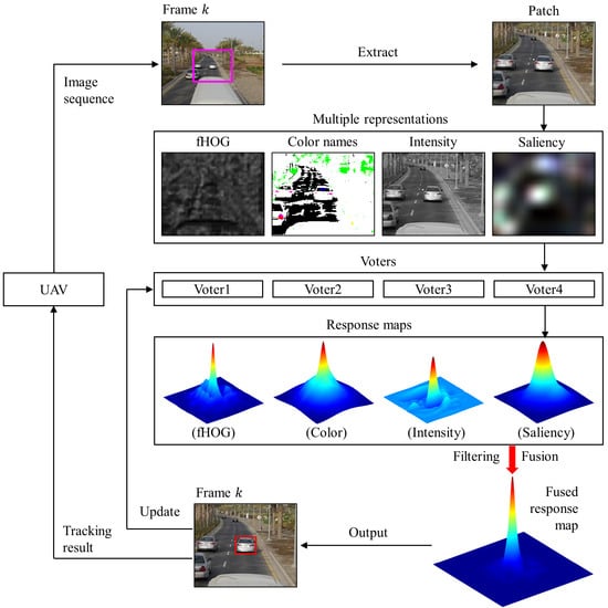
• Novel visual features, i.e., intensity, color names (CN) [31] and saliency [32], for background-aware correlation filter framework to achieve tracking: In original background-aware correlation filter framework, HOG is used as the feature to conduct object tracking. It is difficult to obtain comprehensive information of objects or background using a single feature, especially in aerial tracking.
• A new strategy for fusing response maps which learned from related multiple features: A simple yet effective fusion strategy that effectively combines different response maps is designed. In the challenging tracking sequences with various changes, the response from a single feature may contain interference information, which should be filtered before the fusion. To make the interference information filtering more accurate and adaptive, the peak to sidelobe ratio (PSR) is used to measure the peak strength of the response and weight the response map. In addition, the weighting approach is able to gradually enhance the response level for the final fusion map.
• Qualitative and quantitative experiments on 123 challenging UAV image sequences, i.e., UAV123 [17], show that the presented tracking approach, i.e., OMFL tracker, achieves real-time performance on an i7 processor (3.07 GHz) with 32 GB RAM and performs favorably against 13 state-of-the-art trackers in terms of robustness, accuracy, and efficiency.

To the best of our knowledge, the OMFL tracker has not been designed for the object tracking and employed in the UAV tracking applications in literature.

The remainder of this paper is organized below: Section 2 introduces the related works. Section 3 presents the general framework of the presented tracking approach, i.e., OMFL tracker, and its main modules. Section 4 shows qualitative and quantitative experimental results with different voters, OMFL tracker and the state-of-the-art tracking approaches. Section 5 concludes on the presented visual tracker.

2. Related Works

This section introduces the state-of-the-art tracking approaches, which are closely related to this work.

2.1. Tracking with Discriminative Method

The discriminative method is to use a discriminative appearance model for handling object appearance changes during tracking. This method consists of training and updating a classifier online to distinguish the object (i.e., foreground) from object background. In this method, a classifier is tested on a number of candidate samples to find the most likely location, and updated according to the new input samples which contain positive and negative samples. Hare et al. [33] proposed a tracking algorithm based on a structured learning approach, i.e., STRUCK tracker. It directly predicts the object location change between frames and avoids the label prediction problem in common online classifiers. To utilize the underlying structure of positive and negative samples, Kalal et al. [19] proposed a tracking-learning-detection (TLD) method, i.e., TLD tracker, to guide the sampling process by selecting relevant samples from each new image, and update classifier for object tracking. Inspired by compressive sensing technique, Zhang et al. [21] proposed an approach, i.e., CT tracker, for projecting positive and negative samples to a fixed random basis, and then a naive Bayes classifier is trained for tracking. Moreover, Babenko et al. [20] introduced multiple-instance learning (MIL) into online tracking, i.e., MIL tracker. The samples in the MIL tracker are presented in bags, and labels are provided for the bags instead of individual instances. Although these discriminative trackers have made great progress for visual tracking, the CF-based trackers have shown better performance in fast object tracking and are more robust to the challenging situations such as motion blur and illumination changes.

2.2. Tracking with Correlation Filter

Tracking approach with the CF has attracted a great number of attention because of its high computational efficiency, accuracy, and robustness. Bolme et al. [22] derived a fast correlation filter, i.e., MOSSE tracker, which utilizes classical signal processing analysis and contains a minimum output sum of squared errors filter. Henriques et al. [23] designed kernel classifiers with the same characteristics as correlation filters, i.e., CSK tracker. The kernelized least-squares classifier in the CSK tracker can be trained and evaluated by fast Fourier transform. Based on the framework of CSK tracker, Danelljan et al. [24] introduced color attributes and proposed an adaptive dimension reduction technique, which can preserve useful information while greatly reducing the number of color dimensions. In [25], Henriques et al. combined techniques of kernel trick and circulant matrix to train kernelized correlation filter (KCF), i.e., KCF tracker, with HOG feature. The KCF tracker has more adaptive performance for different scenarios by using multi-channel HOG feature. Moreover, Li et al. proposed a scale adaptive kernel correlation filter, i.e., SAMF tracker [26], which integrates the HOG and CN [31] features, thereby learning a model that is inherently robust to both deformations and illumination changes. However, the synthetic negative samples, which are generated by the circular shift over the object, are used in the filter training stage. In addition, the aforementioned trackers have the boundary effect problem in the training and detection stages, which significantly influences the tracking performance.

2.3. Tracking for Reducing Boundary Effect

In literature, the CFs with limited boundaries (CFLB), i.e., CFLB tracker [28], has learned the CFs for the object tracking with less boundary effect. It has achieved promising tracking results, but the pixel intensities are used as the only feature for learning CFs in the CFLB. In other words, the pixel intensities are not enough to represent the object appearance under the challenging situations for obtaining a more robust tracking performance. The CFs with spatial regularization, i.e., SRDCF tracker [27], has learned the CFs with spatial constraints for the object tracking. Its main drawback is that it cannot be used for the real-time tracking applications due to the highly-cost regularization operation, especially in the UAV tracking tasks. In addition, Galoogahi et al. [29] proposed a background-aware correlation filter with HOG feature, i.e., BACF tracker, which is able to learn and train filters from real negative examples sampled from the object background. It addresses the lack of real negative training samples and is unlike the aforementioned CF-based trackers, which are using the circular shifted patches as the negative samples. It achieves better tracking performances in terms of accuracy, efficiency, and robustness in comparison with above CF-based trackers. Therefore, the background-aware correlation filter framework is adopted to conduct the object tracking applications for the UAV in this work. However, it is still difficult to obtain comprehensive information of object or background using a single feature type, especially for aerial tracking in complex environments with challenging factors as discussed in Section 1. Thus, online multi-feature learning approach is designed to enhance the robustness for various object appearance changes, and ensure the tracking accuracy in real-time aerial tracking.

3. Proposed Tracking Approach

3.1. Overview

In this section, the main structure of the presented online multi-feature learning approach based on background-aware correlation filter framework is introduced. The main steps of the proposed tracking method are illustrated in Figure 1. Given an image, different features from the search window patch centered at the estimated object position in the previous image frame are extracted. In the proposed method, different features, including fHOG [33], CN, intensity, and saliency, are incorporated into the background-aware correlation filter framework to establish four different voters, i.e., Voter1, Voter2, Voter3, and Voter4. With these four voters, the response maps corresponding to each feature can be obtained. After obtained individual response maps, these different response maps are fused with the proposed fusion strategy to get a more accurate and more salient response map with less noise. The fusion strategy includes noise removal and fusion operations. In the fusion process, the PSR is applied to measure the peak sharpness of each response map and weight the response values. By forming a weighted operation of different response maps, the final fused response map can be achieved. Therefore, the tracking result of the current frame can be inferred by searching the highest response value in the final fusion map.

Remark 1.

It is noted that different voters are trained and updated with the samples extracted from the previous image frame. In addition, response maps generated from different voters provide different values, i.e., confidences, to locate the object.

3.2. Tracking with Background-Aware Correlation Filter

The classical correlation filter tracker trains a classifier by minimizing the objective function $\mathcal{E}\left(\mathbf{w}\right)$ to obtain the optimal parameters of filter $\mathbf{w}$:

$$\mathcal{E}\left(\mathbf{w}\right)=\frac{1}{2}\parallel \mathbf{y}-\sum _{d=1}^D{\mathbf{w}}_d★{\mathbf{x}}_d{\parallel }_2^2+\frac{\lambda }{2}\sum _{d=1}^D{\parallel {\mathbf{w}}_d\parallel }_2^2,$$

(1)

where $\mathcal{E}\left(\mathbf{w}\right)$ is a square error sum between the correlation response of samples ${\mathbf{x}}_d$ and their $M\times 1$ desired correlation response $\mathbf{y}$. ${\mathbf{x}}_d\in {\mathbb{R}}^M$ and ${\mathbf{w}}_d\in {\mathbb{R}}^M$ are the vectorized image features and filter, respectively. The subscript d denotes the d-th one of D feature channels. $\lambda$ is a regularization parameter, and ★ denotes the spatial correlation operator.

Remark 2.

The trackers with classical CFs are greatly affected by boundary effect, which leads to suboptimal tracking performance. Specifically, the input samples are weighted by a cosine window to alleviate the edge discontinuity of images caused by the boundary effect, thereby reducing the appearance of the input samples and resulting in the limitation of the object search region in the detection stage of classical CFs. In addition, the classical CF-based trackers use the inaccurate negative training samples, i.e., synthetic samples, as shown in Figure 2. Moreover, they discard the visual information of real background in the training stage. Consequently, the capability to distinguish cluttered background is decreased, which increases the risk of detection failure when objects are sharing similar visual cues to the surrounding background.

Different from the classical CF, the background-aware correlation filter [29] applies a circular shift operator and a cropping operator on the image, as the illustration shown in Figure 3. This approach trains a filter that can better distinguish foreground object from its shifted samples. The background-aware correlation filter $\mathbf{w}$ is trained by minimizing the following objective:

$$\mathcal{E}\left(\mathbf{w}\right)=\frac{1}{2}\sum _{j=1}^N{\left(\mathbf{y}\left(j\right)-\sum _{d=1}^D{\mathbf{w}}_d^{\top }\mathbf{B}{\mathbf{x}}_d[\Delta {\mathbf{\tau }}_j]\right)}^2+\frac{\lambda }{2}\sum _{d=1}^D{\parallel {\mathbf{w}}_d\parallel }_2^2,$$

(2)

where $\mathcal{E}\left(\mathbf{w}\right)$ is a squared error sum over response of sample ${\mathbf{Bx}}_d[\Delta {\mathbf{\tau }}_j]$ and its regression target $\mathbf{y}\left(j\right)$. $\mathbf{B}\in {\mathbb{R}}^{M\times N}$ is a binary matrix that can crop the middle M elements of signal ${\mathbf{x}}_d$ with size N, i.e., ${\mathbf{x}}_d\in {\mathbb{R}}^{N\times 1}$, where $N\gg M$. $[\Delta {\mathbf{\tau }}_j]$ is the circular shift operator, and ${\mathbf{x}}_d[\Delta {\mathbf{\tau }}_j]$ means circularly shifting the elements in the signal ${\mathbf{x}}_d$ by j positions. Therefore, ${\mathbf{Bx}}_d[\Delta {\mathbf{\tau }}_j]$ returns all shifted signals with the size of M from signal ${\mathbf{x}}_d$. The superscript ⊤ denotes the conjugate transpose of a complex vector or matrix.

Remark 3.

It is noted that the background-aware correlation filter uses the real negative samples for the training instead of using the synthetic negative samples, as the illustration in Figure 3.

In order to improve the computational efficiency, correlation filters are typically learned in the frequency domain. Equation (2) can be converted to an expression in the frequency domain:

$$\begin{array}{c}\hfill \mathcal{E}(\mathbf{w},\widehat{\mathbf{g}})=\frac{1}{2}\parallel \widehat{\mathbf{y}}-\widehat{\mathbf{X}}\widehat{\mathbf{g}}{\parallel }_2^2+\frac{\lambda }{2}{\parallel \mathbf{w}\parallel }_2^2\\ \hfill s.t.\widehat{\mathbf{g}}=\sqrt{N}({\mathbf{I}}_D\otimes \mathbf{F}{\mathbf{B}}^{\top })\mathbf{w},\end{array}$$

(3)

where $\widehat{\mathbf{X}}\in {\mathbb{C}}^{N\times DN}$, $\widehat{\mathbf{g}}\in {\mathbb{C}}^{DN\times 1}$ and $\mathbf{w}\in {\mathbb{R}}^{DM\times 1}$ are defined as $\widehat{\mathbf{X}}=[diag{\left({\widehat{\mathbf{x}}}_1\right)}^{\top },\cdots ,diag{\left({\widehat{\mathbf{x}}}_D\right)}^{\top }]$, $\widehat{\mathbf{g}}={[{\widehat{\mathbf{g}}}_1^{\top },\cdots ,{\widehat{\mathbf{g}}}_D^{\top }]}^{\top }$ and $\mathbf{w}={[{\mathbf{w}}_1^{\top },\cdots ,{\mathbf{w}}_D^{\top }]}^{\top }$, respectively. ${\mathbf{I}}_D\in {\mathbb{R}}^{D\times D}$ is a identify matrix and ⊗ denotes the Kronecker product. The superscript $\widehat{}$ indicates the discrete Fourier transform of a signal, i.e., $\widehat{\mathbf{\alpha }}=\sqrt{N}\mathbf{F}\mathbf{\alpha }$. $\mathbf{F}\in {\mathbb{C}}^{N\times N}$ is the orthonormal matrix for mapping any N dimensional vectorized signal to the Fourier domain.

To solve Equation (3), an augmented lagrangian method [34] is employed:

$$\begin{array}{cc}\hfill \mathcal{L}(\mathbf{w},\widehat{\mathbf{g}},\widehat{\mathbf{\zeta }})=& \frac{1}{2}\parallel \widehat{\mathbf{y}}-\widehat{\mathbf{X}}\widehat{\mathbf{g}}{\parallel }_2^2+\frac{\lambda }{2}{\parallel \mathbf{w}\parallel }_2^2\hfill \\ & +{\widehat{\mathbf{\zeta }}}^{\top }\left(\widehat{\mathbf{g}}-\sqrt{N}({\mathbf{I}}_D\otimes \mathbf{F}{\mathbf{B}}^{\top })\mathbf{w}\right)\hfill \\ & +\frac{\mu }{2}{\parallel \widehat{\mathbf{g}}-\sqrt{N}({\mathbf{I}}_D\otimes \mathbf{F}{\mathbf{B}}^{\top })\mathbf{w}\parallel }_2^2,\hfill \end{array}$$

(4)

where $\mu$ is a penalty factor and $\widehat{\mathbf{\zeta }}\in {\mathbb{C}}^{DN\times 1}$ is the lagrangian vector in the Fourier domain defined as $\widehat{\mathbf{\zeta }}={[{\widehat{\mathbf{\zeta }}}_1^{\top },\cdots ,{\widehat{\mathbf{\zeta }}}_D^{\top }]}^{\top }$.

To handle with Equation (4), the alternating direction method of multipliers, i.e., ADMM [34], technique is used. Each of the subproblems, i.e., ${\mathbf{w}}^{*}$ and ${\widehat{\mathbf{g}}}^{*}$, has an analytic solution.

For subproblem ${\mathbf{w}}^{*}$:

$${\mathbf{w}}^{*}={(\mu +\frac{\lambda }{N})}^{-1}(\mu \mathbf{g}+\mathbf{\zeta }),$$

(5)

where $\mathbf{g}=\frac{1}{\sqrt{N}}({\mathbf{I}}_D\otimes \mathbf{B}{\mathbf{F}}^{\top })\widehat{\mathbf{g}}$ and $\mathbf{\zeta }=\frac{1}{\sqrt{N}}({\mathbf{I}}_D\otimes \mathbf{B}{\mathbf{F}}^{\top })\widehat{\mathbf{\zeta }}$.

For subproblem ${\widehat{\mathbf{g}}}^{*}$, it can be solved by solving N independent objectives, i.e., ${\widehat{\mathbf{g}}}^{*}\left(j\right)$, where $j=[1,\cdots ,N]$:

$$\begin{array}{cc}\hfill {\widehat{\mathbf{g}}}^{*}\left(j\right)=& \frac{1}{\mu }\left(N\widehat{\mathbf{y}}\left(j\right)\widehat{\mathbf{x}}\left(j\right)-\widehat{\mathbf{\zeta }}\left(j\right)+\mu \widehat{\mathbf{w}}\left(j\right)\right)\hfill \\ & -\frac{\widehat{\mathbf{x}}\left(j\right)}{\mu b}\left(N\widehat{\mathbf{y}}\left(j\right)\widehat{\mathbf{x}}{\left(j\right)}^{\top }\widehat{\mathbf{x}}\left(j\right)-\widehat{\mathbf{x}}{\left(j\right)}^{\top }\widehat{\mathbf{\zeta }}\left(j\right)+\mu \widehat{\mathbf{x}}{\left(j\right)}^{\top }\widehat{\mathbf{w}}\left(j\right)\right),\hfill \end{array}$$

(6)

where $\widehat{\mathbf{x}}\left(j\right)={[{\widehat{\mathbf{x}}}_1\left(j\right),\cdots ,{\widehat{\mathbf{x}}}_D\left(j\right)]}^{\top }$ and $\widehat{\mathbf{w}}\left(j\right)={[{\widehat{\mathbf{w}}}_1\left(j\right),\cdots ,{\widehat{\mathbf{w}}}_D\left(j\right)]}^{\top }$. Note that $\widehat{\mathbf{y}}\left(j\right)$, ${\widehat{\mathbf{x}}}_d\left(j\right)$ and ${\widehat{\mathbf{w}}}_d\left(j\right)$ are elements of $\widehat{\mathbf{y}}$, ${\widehat{\mathbf{x}}}_d$ and ${\widehat{\mathbf{w}}}_d$, respectively. ${\widehat{\mathbf{w}}}_d=\sqrt{N}\mathbf{F}{\mathbf{B}}^{\top }{\mathbf{w}}_d$ and $b=\widehat{\mathbf{x}}{\left(j\right)}^{\top }\widehat{\mathbf{x}}\left(j\right)+N\mu$ is a scalar quantity.

The lagrangian vector is updated by the function:

$${\widehat{\mathbf{\zeta }}}^{(i+1)}={\widehat{\mathbf{\zeta }}}^{\left(i\right)}+\mu ({\widehat{\mathbf{g}}}^{(i+1)}-{\widehat{\mathbf{w}}}^{(i+1)}),$$

(7)

where ${\widehat{\mathbf{w}}}^{(i+1)}=({\mathbf{I}}_D\otimes \mathbf{F}{\mathbf{B}}^{\top }){\mathbf{w}}^{(i+1)}$ and the superscript $(i+1)$ represents the $(i+1)$-th iteration of the iterative ADMM algorithm. A common scheme for choosing the penalty factor $\mu$ is ${\mu }^{(i+1)}=min({\mu }_{max},\beta {\mu }^{\left(i\right)})$ [34].

Similar to other CF-based trackers, an online adaptation strategy is used to improve the robustness to various appearance changes. The online adaptation at frame k is formulated as:

$${\widehat{\mathbf{x}}}_{model}^{\left(k\right)}=(1-\eta ){\widehat{\mathbf{x}}}_{model}^{(k-1)}+\eta {\widehat{\mathbf{x}}}^{\left(k\right)},$$

(8)

where $\eta$ is the online adaptation rate.

Remark 4.

It is noted that the background-aware correlation filter uses the HOG feature to represent the object. However, it is easy to cause the tracking failure when the texture information of the object becomes blurred. For a tracking problem, features should have the capability to deal with changes of tracking object and background, such as deformation, motion blur, illumination and rotation variations. Therefore, different features are selected instead of using only one and propose an effective response map fusion strategy to improve the tracking performance in different scenarios.

3.3. Object Representation with Multiple Features

In the presented approach, the features from different clues, i.e., texture, color, gray value, and saliency, which respectively correspond to features of fHOG [33], CN [31], intensity and saliency [32], are selected.

3.3.1. Object Representation with fHOG

For the HOG [30], it captures edge or gradient structure, which is highly characteristic of local shape. It is expressed by local representations, which has the advantage of invariance to local geometric and photometric transformations. If the translations or rotations are much smaller than the size of orientation bin, there is no much difference on the object representation. Moreover, even without precise knowledge of the corresponding gradient or edge positions, local object appearance and shape can be well characterized by the distribution of local intensity gradients or edge directions.

Remark 5.

Considering that the dimensionality of HOG feature [30] can be significantly reduced with no noticeable loss of information, a lower dimensional HOG feature, i.e., fHOG [33] has been used in this work. In addition, the integration of the fHOG feature and background-aware correlation filter framework denotes as the Voter1 in this work.

Given an image frame $I^{\left(k\right)}$, the steps to extract the fHOG feature are summarized in Algorithm 1.

Algorithm 1: fHOG feature extraction

Input: $I^{\left(k\right)}$  1 Convert $I^{\left(k\right)}$ to the grayscale intensity image  2 Calculate the gradient of each pixel to get a pixel-level feature map $P^{\left(k\right)}$  3 Aggregate $P^{\left(k\right)}$ into a dense grid of rectangular cells to obtain a cell-based feature map $C^{\left(k\right)}$, where the cell size is set to $c\times c$  4 Truncate and normalize $C^{\left(k\right)}$ by using four different normalization factors of a 27-dimensional histogram over nine insensitive orientations and 18 sensitive orientations  5 Sum on each orientation channel with different normalization factors  6 Sum on the values of nine contrast insensitive orientations based on each normalization factor     Output: fHOG feature ${\mathcal{H}}^{\left(k\right)}$

3.3.2. Object Representation with Color Names

In addition to the texture information, color attributes, which perform well in image retrieval [31], can also be used to describe the characteristics of the object. Color attributes are also referred to as color names, i.e., CN, which can cope well with object deformation and variation in shape. The operation of building color names of the object is to associate RGB observations with the preselected set of 11 basic color terms, i.e., 11 linguistic color labels. To achieve the CN feature, the image $I^{\left(k\right)}$ is firstly resized to $I_{re}^{\left(k\right)}$ with the same size of $C^{\left(k\right)}$. Then, the mapping method provided by [31], which maps the RGB values to an 11-dimensional color representation ${\mathcal{C}}^{\left(k\right)}$, is used to achieve the feature extracted from $I_{re}^{\left(k\right)}$. ${\mathcal{C}}^{\left(k\right)}$ is represented by a histogram that indicates how many pixels are allocated to each bin, i.e., color name. Figure 4 shows the pixel-wise color name annotation map, where the color names are represented by their corresponding color.

Remark 6.

In this work, the set of eleven basic color English terms [35] are used as color names, including black, blue, brown, gray, green, orange, pink, purple, red, white and yellow. Additionally, the combination of the CN feature and background-aware correlation filter framework denotes as the Voter2 in this work.

3.3.3. Object Representation with Pixel Intensity

In real UAV tracking applications, when the colors of the pixels representing the object and its background are similar, the mapping during the extraction of the CN feature may cause them to have the same color name. Therefore, the intensity feature, which retains the nuance between the object and background, is taken into account to improve UAV tracking performance. In this work, gray value, which is robust to motion blur, is utilized to make up the intensity feature. Similarly, the image $I^{\left(k\right)}$ is resized to $I_{re}^{\left(k\right)}$ with the same size of $C^{\left(k\right)}$ firstly. The intensity feature ${\mathcal{G}}^{\left(k\right)}$ can be obtained by converting RGB values of $I_{re}^{\left(k\right)}$ to gray values. By forming a weighted sum of the three channels values of $I_{re}^{\left(k\right)}$, i.e., red, green and blue components, Equation (9) is employed to calculate the gray value of the $(i,j)$’s element in ${\mathcal{G}}^{\left(k\right)}$:

$${\mathcal{G}}^{\left(k\right)}(i,j)={\alpha }_R{I}_{re,R}^{\left(k\right)}(i,j)+{\alpha }_G{I}_{re,G}^{\left(k\right)}(i,j)+{\alpha }_B{I}_{re,B}^{\left(k\right)}(i,j),$$

(9)

where $I_{re,R}^{\left(k\right)}$, $I_{re,G}^{\left(k\right)}$ and $I_{re,B}^{\left(k\right)}$ denote the red, green and blue components of $I_{re}^{\left(k\right)}$, respectively. The process of the conversion is shown in Figure 5.

Remark 7.

It is noted that ${\alpha }_R$, ${\alpha }_G$ and ${\alpha }_B$ are set to 0.2989, 0.5870 and 0.1140 in this work, respectively. In addition, the intensity feature is incorporated into the background-aware correlation filter framework to achieve the Voter3.

3.3.4. Object Representation with Saliency

Saliency is usually used in object detection, which takes advantage of the fact that an object is more noticeable than its background. Therefore, the object with saliency information is used to enhance object tracking in this work. Inspired by [32], the spectra residual approach to extract saliency feature of the resized image $I_{re}^{\left(k\right)}$ is utilized, as an example shown in Figure 6.

Before extracting the saliency feature, the image $I_{re}^{\left(k\right)}$ is preprocessed. As shown in Equations (10) and (11), the Fourier transform $\mathcal{F}$ is used to obtain the amplitude feature ${\mathbf{A}}^{\left(k\right)}$ and phase feature ${\mathbf{P}}^{\left(k\right)}$ of $I_{re}^{\left(k\right)}$ in the frequency domain:

$${\mathbf{A}}^{\left(k\right)}=A\left(\mathcal{F}\left(I_{re}^{\left(k\right)}\right)\right),$$

(10)

$${\mathbf{P}}^{\left(k\right)}=P\left(\mathcal{F}\left(I_{re}^{\left(k\right)}\right)\right).$$

(11)

Instead of using the log-log representation, the log spectrum representation ${\mathbf{L}}^{\left(k\right)}$ of the image $I_{re}^{\left(k\right)}$ is adopted, it can be obtained by:

$${\mathbf{L}}^{\left(k\right)}=log\left({\mathbf{A}}^{\left(k\right)}\right).$$

(12)

The amplitude feature ${\mathbf{A}}^{\left(k\right)}$ can be approximated by the convolution between ${\mathbf{H}}_n$ and ${\mathbf{L}}^{\left(k\right)}$. Therefore, the spectral residual ${\mathbf{r}}^{\left(k\right)}$ can be achieved by Equation (13):

$${\mathbf{r}}^{\left(k\right)}={\mathbf{L}}^{\left(k\right)}-{\mathbf{H}}_n★{\mathbf{L}}^{\left(k\right)},$$

(13)

where ★ denotes convolution operator, and ${\mathbf{H}}_n$ is an $n\times n$ matrix defined by:

$${\mathbf{H}}_n=\frac{1}{n^2}\left[\begin{array}{cccc}1& 1& \cdots & 1\\ 1& 1& \cdots & 1\\ ⋮& ⋮& \ddots & ⋮\\ 1& 1& \cdots & 1\end{array}\right].$$

The noticeable information contained in an image can be captured by a spectral residual ${\mathbf{r}}^{\left(k\right)}$. In other words, ${\mathbf{r}}^{\left(k\right)}$ can be understood as a compressed representation of an underlying scene that the image reflects. The saliency map in the spatial domain by employing inverse Fourier transform ${\mathcal{F}}^{-1}$ can be obtained. Given the image $I_{re}^{\left(k\right)}$, the saliency map can be achieved by:

$${\mathcal{S}}^{\left(k\right)}={\mathbf{G}}^{\left(k\right)}★{\mathcal{F}}^{-1}{\left[exp\left({\mathbf{r}}^{\left(k\right)}+{\mathbf{P}}^{\left(k\right)}\right)\right]}^2,$$

(14)

where ${\mathbf{G}}^{\left(k\right)}$ is a Gaussian filter smoothing the saliency map for better visual effects.

Remark 8.

It is noted that changing the size of ${\mathbf{H}}_n$ has only a slight effect on the result, thus n is empirically set to 3 in this work. The size and variance of the Gaussian filter ${\mathbf{G}}^{\left(k\right)}$ is set to $10\times 10$ and 2.5, respectively. In addition, Voter4 is implemented by integrating the saliency feature and the background-aware correlation filter framework.

3.4. Fusion of Multi-Feature Learning

In the challenging tracking sequences with various object appearance changes, it is not enough to use one feature to express object information. To enhance the tracking performance, a simple yet effective strategy to combine different features is designed in this work. Given an image frame $I^{\left(k\right)}$ and the voter V, the response maps on each feature can be obtained as:

$$R^{f^{\left(k\right)}}=V\left(I^{\left(k\right)}\right),$$

(15)

where $f^{\left(k\right)}\in \{{\mathcal{H}}^{\left(k\right)},{\mathcal{C}}^{\left(k\right)},{\mathcal{G}}^{\left(k\right)},{\mathcal{S}}^{\left(k\right)}\}$. $\mathcal{H}$, $\mathcal{C}$, $\mathcal{G}$ and $\mathcal{S}$ denote the fHOG, CN, intensity and saliency features, respectively.

Remark 9.

If the different response maps are fused without any preprocessing, the variant interference information will make the fused response maps inevitably contain the noise. Therefore, the PSR is used to measure the peak strength of the response $R^{f^{\left(k\right)}}$ and weight $R^{f^{\left(k\right)}}$ in this work, as one example show in Figure 7.

The processed response map ${\mathcal{R}}^{f^{\left(k\right)}}$ can be obtained by Equation (16):

$${\mathcal{R}}^{f^{\left(k\right)}}={\omega }_1^{f^{\left(k\right)}}{R}^{f^{\left(k\right)}},$$

(16)

where ${\omega }_1^{f^{\left(k\right)}}$ is defined as:

$${\omega }_1^{f^{\left(k\right)}}=\frac{max\left(R^{f^{\left(k\right)}}\right)-{\mu }_1^{f^{\left(k\right)}}}{{\sigma }_1^{f^{\left(k\right)}}},$$

(17)

where ${\mu }_1^{f^{\left(k\right)}}$ and ${\sigma }_1^{f^{\left(k\right)}}$ are mean and standard deviation of $R^{f^{\left(k\right)}}$, respectively.

To make the noise filtering more accurate and adaptive, the proposed fusion strategy is used to integrate the information contained in different ${\mathcal{R}}^{f^{\left(k\right)}}$:

$${\mathcal{R}}^{f_1^{\left(k\right)}{f}_2^{\left(k\right)}}={\mathcal{R}}^{f_1^{\left(k\right)}}\odot {\mathcal{R}}^{f_2^{\left(k\right)}},$$

(18)

where $f_1^{\left(k\right)}\ne f_2^{\left(k\right)}$ and ⊙ denotes the element-wise product. Therefore, Equation (18) means the processed response map ${\mathcal{R}}^{f_1^{\left(k\right)}}$ is weighted by ${\mathcal{R}}^{f_2^{\left(k\right)}}$. After the fusion between all the pair combinations of the response maps, six fused response maps, i.e., ${\mathcal{R}}^{{\mathcal{H}}^{\left(k\right)}{\mathcal{C}}^{\left(k\right)}}$, ${\mathcal{R}}^{{\mathcal{H}}^{\left(k\right)}{\mathcal{G}}^{\left(k\right)}}$, ${\mathcal{R}}^{{\mathcal{H}}^{\left(k\right)}{\mathcal{S}}^{\left(k\right)}}$, ${\mathcal{R}}^{{\mathcal{C}}^{\left(k\right)}{\mathcal{G}}^{\left(k\right)}}$, ${\mathcal{R}}^{{\mathcal{C}}^{\left(k\right)}{\mathcal{S}}^{\left(k\right)}}$ and ${\mathcal{R}}^{{\mathcal{G}}^{\left(k\right)}{\mathcal{S}}^{\left(k\right)}}$, which have more salient confidences in response maps, can be achieved, as shown in Figure 8.

In order to make better use of each fused response map and highlight the information in each response map, the following formula is used for the final fusion $\mathcal{Q}$:

$$\begin{array}{cc}{\mathcal{Q}}^{\left(k\right)}=\frac{1}{6}\hfill & ({\omega }_2^{{\mathcal{H}}^{\left(k\right)}{\mathcal{C}}^{\left(k\right)}}{\mathcal{R}}^{{\mathcal{H}}^{\left(k\right)}{\mathcal{C}}^{\left(k\right)}}\oplus {\omega }_2^{{\mathcal{H}}^{\left(k\right)}{\mathcal{G}}^{\left(k\right)}}{\mathcal{R}}^{{\mathcal{H}}^{\left(k\right)}{\mathcal{G}}^{\left(k\right)}}\oplus {\omega }_2^{{\mathcal{H}}^{\left(k\right)}{\mathcal{S}}^{\left(k\right)}}{\mathcal{R}}^{{\mathcal{H}}^{\left(k\right)}{\mathcal{S}}^{\left(k\right)}}\hfill \\ & \oplus {\omega }_2^{{\mathcal{C}}^{\left(k\right)}{\mathcal{G}}^{\left(k\right)}}{\mathcal{R}}^{{\mathcal{C}}^{\left(k\right)}{\mathcal{G}}^{\left(k\right)}}\oplus {\omega }_2^{{\mathcal{C}}^{\left(k\right)}{\mathcal{S}}^{\left(k\right)}}{\mathcal{R}}^{{\mathcal{C}}^{\left(k\right)}{\mathcal{S}}^{\left(k\right)}}\oplus {\omega }_2^{{\mathcal{G}}^{\left(k\right)}{\mathcal{S}}^{\left(k\right)}}{\mathcal{R}}^{{\mathcal{G}}^{\left(k\right)}{\mathcal{S}}^{\left(k\right)}}),\hfill \end{array}$$

(19)

where ⊕ stands for element-wise addition and ${\omega }_2^{f_1^{\left(k\right)}{f}_2^{\left(k\right)}}$ is defined as:

$${\omega }_2^{f_1^{\left(k\right)}{f}_2^{\left(k\right)}}=\frac{max\left({\mathcal{R}}^{f_1^{\left(k\right)}{f}_2^{\left(k\right)}}\right)-{\mu }_2^{f^{f_1^{\left(k\right)}{f}_2^{\left(k\right)}}}}{{\sigma }_2^{f^{f_1^{\left(k\right)}{f}_2^{\left(k\right)}}}},$$

(20)

where ${\mu }_2^{f^{f_1^{\left(k\right)}{f}_2^{\left(k\right)}}}$ and ${\sigma }_2^{f^{f_1^{\left(k\right)}{f}_2^{\left(k\right)}}}$ are mean and standard deviation of ${\mathcal{R}}^{f_1^{\left(k\right)}{f}_2^{\left(k\right)}}$, respectively. Therefore, the final fused response map can be implemented, as shown in Figure 8, where the highest value is the result of the detection.

Remark 10.

It is noted that the strategy to achieve the final fused response map ${\mathcal{Q}}^{\left(k\right)}$ mainly utilizes two operations, i.e., noise removal and fusion. Weighted fusion using PSR is more preferable than direct fusion without pre-treatment. With the PSR-based weighting operation, most of the interference information can be effectively filtered in the fusion process. Therefore, the final fused response map can be obtained with more salient confidences but less noise, as shown in Figure 8.

The pseudocode of the OMFL tracker is summarized in Algorithm 2.

Algorithm 2: OMFL tracker

4. Evaluation of Tracking Performance

4.1. Evaluation Criteria

To analyze and evaluate the performance of the proposed tracking approach, i.e., OMFL tracker, center location error (CLE) and success rate (SR) [36] based on one-pass evaluation are employed as the main evaluation criteria in this work.

For the CLE, it is measured as the Euclidean distance in pixels between the center of the estimated object bounding box and the corresponding ground truth center, which is defined as:

$$\mathrm{CLE}=\parallel O_E^{\left(k\right)}-O_{GT}^{\left(k\right)}\parallel ,$$

(21)

where $O_E^{\left(k\right)}$ and $O_{GT}^{\left(k\right)}$ are the center of the estimated object bounding box and the corresponding ground truth center, respectively. To preferably show the tracking performance with CLE, precision plot (PP) is used. For each value $\xi$ on the PP, it is defined as the ratio between the number of frames whose CLE is smaller than $\xi$, i.e., $N_{\mathrm{CLE}<\xi }$, and the total number of image frames $N_{\mathrm{Total}}$.

$$\mathrm{PP}\left(\xi \right)=\frac{N_{\mathrm{CLE}<\xi }}{N_{\mathrm{Total}}}.$$

(22)

For the SR, it represents the percentage between the successful tracking frames with the total number of image frames. If an image frame is a success, its overlap score (OS) is larger than a given threshold. For the OS, it is defined as below:

$$\mathrm{OS}=\frac{|r_E^{\left(k\right)}\cap r_{GT}^{\left(k\right)}|}{|r_E^{\left(k\right)}\cup r_{GT}^{\left(k\right)}|},$$

(23)

where $r_E^{\left(k\right)}$ and $r_{GT}^{\left(k\right)}$ stand for the regions of the estimated and ground-truth object bounding boxes, respectively. ∩ and ∪ denote the intersection and union operators. $|*|$ is the number of pixels in the intersection or union region. In this work, success plot (SP) is employed to show the tracking performance. For each value $\eta$ on the SP, it is defined as the ratio between the number of frames whose OS is larger than $\eta$, i.e., $N_{\mathrm{OS}>\eta }$, and the total number of image frames $N_{\mathrm{Total}}$.

$$\mathrm{SP}\left(\eta \right)=\frac{N_{\mathrm{OS}>\eta }}{N_{\mathrm{Total}}}.$$

(24)

Remark 11.

In the evaluation of all visual trackers, $\xi =20$ on each PP and area under curve (AUC) of each SP are used for ranking of tracking performance.

4.2. Overall Performance

In this section, 123 challenging aerial image sequences (including 37,885 image frames), i.e., UAV123 [17], are used to evaluate the overall performance of the proposed online learning tracking approach, i.e., OMFL tracker, and other state-of-the-art trackers. Especially, two different types of evaluations have been setup.

4.2.1. Evaluation with Different Voters

As shown in Figure 1, different Voters, which have respectively integrated fHOG, CN, intensity and saliency with the background-aware correlation filter framework, have been presented, i.e., Voter1, Voter2, Voter3, and Voter4. To evaluate the OMFL tracker, these four Voters have been used to conduct the comparisons with the OMFL tracker in terms of precision and success rate, as shown in Figure 9.

As can be seen from the PPs in Figure 9, the scores of PPs (i.e., $\xi =20$) are 0.655, 0.587, 0.548, 0.481 and 0.420 for the OMFL tracker, Voter1, Voter2, Voter3 and Voter4, respectively. Therefore, the OMFL tracker has achieved the best tracking performance in terms of precision. Similarly, the scores of SPs (i.e., AUCs of SPs) are 0.459, 0.423, 0.401, 0.351 and 0.296 for the OMFL tracker, Voter1, Voter2, Voter3, and Voter4, respectively. Thus, the OMFL tracker has also obtained the best tracking performance in terms of success rate. In summary, it can be concluded that the OMFL tracker favorably outperforms Voter1, Voter2, Voter3 and Voter4. Additionally, the multi-feature learning approach is superior to the single-feature learning method.

Remark 12.

It is noted that all parameters used in Voter1, Voter2, Voter3, and Voter4 are the same as the parameters in the OMFL tracker to achieve the fair comparison.

4.2.2. Evaluation with Other State-Of-The-Art Trackers

To achieve a comprehensive evaluation, the OMFL tracker is compared with other 13 state-of-the-art trackers, i.e., MCCT [37], MEEM [38], SRDCF [27], BACF [29], MUSTER [39], STRUCK [18], SAMF [26], DSST [40], TLD [19], KCF [25], CSK [23], ASLA [41], and IVT [42].

Remark 13.

For these state-of-the-art tracking algorithms, the source codes or binary programs provided by the authors or UAV123 with default parameters have been utilized in this work. Although some trackers, e.g., MCCT, have also been implemented with convolution features, convolution features often require a very high computing capability for the onboard computer, they are not suitable for the UAV tracking applications. Therefore, this work emphasizes the evaluation and analysis of all trackers with hand-crafted features. For the proposed OMFL tracker, it is implemented in Matlab without any optimizations, its main parameters are listed in

Table 1. Main parameters in the OMFL tracker.

Paramter	Value	Parameter	Value
Cell size $c\times c$	$4\times 4$	Regularization parameter $\lambda$	$0.01$
Number of scales	5	Penalty factor $\mu$	1
Scale step	$1.01$	${\mu }_{max}$	10,000
Number of iterations of ADMM	2	$\beta$	10
Bandwidth of a 2D gaussian function (object size $[h,w]$)	${\displaystyle \frac{\sqrt{wh}}{16}}$	Online adaptation rate $\eta$	$0.013$

. All aforementioned trackers are evaluated on the same computer. In addition, this work strictly complies with the tracker evaluation protocol from the UAV123 and calculates the average performances as the final results in order to conduct a fair comparison.

Figure 10 shows the PPs and SPs of all tracking algorithms on 123 challenging UAV image sequences. In the PPs, the scores of all trackers on 20 pixels are 0.655 (OMFL), 0.596 (MCCT), 0.584 (MEEM), 0.575 (SRDCF), 0.572 (BACF), 0.526 (MUSTER), 0.509 (Struck), 0.465 (SAMF), 0.448 (DSST), 0.415 (TLD), 0.405 (KCF), 0.401 (CSK), 0.363 (ASLA) and 0.304 (IVT), respectively. Therefore, the OMFL tracker has achieved the best precision among all trackers. In the SPs, the AUC-based scores of all trackers are 0.459 (OMFL), 0.433 (MCCT), 0.423 (SRDCF), 0.413 (BACF), 0.380 (MEEM), 0.371 (MUSTER), 0.347 (Struck), 0.326 (SAMF), 0.286 (TLD), 0.286 (DSST), 0.270 (CSK), 0.265 (KCF), 0.250 (ASLA), 0.224 (IVT), respectively. Similarly, the OMFL tracker still ranks No. 1 among all tracking aglorithms. Thus, it can be summarized that the OMFL tracker is better than other 13 state-of-the-art trackers in terms of precison and success ratio.

Besides the aforementioned comparisons, the UAV image sequences are categorized as 12 different types, i.e., aspect ratio change (ARC), background clutter (BC), camera motion (CM), fast motion (FM), full occlusion (FOC), illumination variation (IV), low resolution (LR), out-of-view (OV), partial occlusion (POC), scale variation (SV), similar object (SOB) and viewpoint change (VC), to achieve a thorough tracking performance evaluation.

Table 2. Scores of precision plots ($\xi$ = 20 pixels). Red, blue and green fonts indicate the best, second best and third best performances among all trackers.

	ARC	BC	CM	FM	FOC	IV	LR	OV	POC	SV	SOB	VC
MCCT	49.3	46.9	54.4	36.1	42.1	47.7	45.5	49.3	54.2	54.7	62.7	48.4
MEEM	51.1	51.0	53.3	34.0	41.0	48.1	48.4	46.9	51.6	53.2	62.4	53.3
SRDCF	47.2	38.9	52.7	42.7	41.8	43.6	43.1	49.2	50.4	53.1	58.5	47.4
BACF	47.8	42.5	53.2	40.7	33.6	43.0	43.1	42.1	46.7	52.5	60.5	49.1
MUSTER	43.5	37.5	47.1	30.2	43.9	38.4	45.2	40.7	44.9	49.1	56.0	43.6
Struck	39.9	52.2	43.9	22.2	38.3	41.5	47.8	38.2	44.6	46.0	52.7	42.8
SAMF	39.0	27.4	37.8	33.2	37.9	33.9	32.2	40.9	41.9	44.1	50.3	35.8
DSST	36.1	22.2	34.0	27.7	31.3	33.3	34.5	35.6	38.4	42.4	50.9	35.8
TLD	34.9	28.5	35.4	22.6	28.3	23.3	44.4	28.1	34.5	39.1	48.0	35.1
KCF	30.3	22.3	30.5	21.7	28.1	26.9	30.5	30.9	34.4	37.3	45.3	31.6
CSK	29.3	22.7	30.6	24.8	29.2	27.2	30.9	30.6	32.8	37.5	43.2	29.4
ASLA	29.3	23.8	23.2	17.1	29.3	23.1	33.8	26.3	31.8	35.3	44.4	27.3
IVT	23.2	18.1	18.6	15.0	24.0	19.6	25.5	23.6	26.3	29.3	35.6	24.0
OMFL	57.9	48.4	62.4	54.2	39.7	54.1	50.8	55.2	57.0	61.1	66.4	59.9

and

Table 3. Scores of success plots (AUC). Red, blue and green fonts indicate the best, second best and third best performances among all trackers.

	ARC	BC	CM	FM	FOC	IV	LR	OV	POC	SV	SOB	VC
MCCT	35.7	30.5	40.7	26.0	23.6	34.2	25.7	36.5	37.6	39.6	45.1	36.1
MEEM	32.7	31.1	36.1	23.1	21.1	32.2	24.1	32.5	33.7	34.0	40.3	34.8
SRDCF	34.6	26.3	39.9	31.1	22.9	33.3	23.7	36.8	35.5	39.0	42.1	35.6
BACF	33.4	27.5	39.7	27.5	17.3	31.0	24.8	32.1	32.7	37.4	42.4	35.3
MUSTER	29.9	22.5	33.3	20.3	22.9	28.1	23.5	29.5	30.2	34.3	38.5	31.6
Struck	27.4	33.1	30.4	15.5	19.8	29.0	24.6	28.0	30.0	30.7	34.0	29.1
SAMF	27.4	16.0	27.1	22.0	19.7	23.8	16.6	28.9	28.2	30.6	34.8	26.4
DSST	23.5	13.7	22.5	15.7	15.6	21.0	17.1	24.5	24.6	26.2	31.5	23.1
TLD	23.9	16.3	25.2	14.8	13.5	16.0	24.2	20.2	21.9	26.8	30.1	25.1
KCF	20.2	12.5	20.9	14.5	13.5	18.3	14.7	22.2	22.3	23.8	27.9	21.0
CSK	20.5	13.4	21.4	15.1	15.0	18.9	14.9	22.7	22.0	24.7	28.5	20.3
ASLA	19.4	14.8	15.9	9.9	13.4	18.0	18.6	16.2	20.2	23.8	30.6	19.9
IVT	16.5	10.3	13.3	9.1	11.5	16.2	13.7	15.2	17.0	21.4	25.6	18.4
OMFL	38.9	31.2	44.9	33.9	20.8	35.6	27.8	39.5	38.3	42.2	46.6	41.0

provide the scores of PPs and SPs on above 12 attributes. In the Table 2, the OMFL tracker has better precision scores than other trackers in terms of the ARC, CM, FM, IV, LR, OV, POC, SV, SOB, and VC attributes. For the Table 3, it shows that the OMFL tracker has obtained the best AUC-based scores in terms of the ARC, CM, FM, IV, LR, OV, POC, SV, SOB, and VC attributes. Figure 11 is the analysis of precision scores for all trackers with different attributes. It shows that the OMFL tracker is ranking the No. 1 in general among all trackers. Additionally, Figure 12 is the analysis of AUC-based scores for all trackers with different attributes. It indicates that the OMFL tracker is also ranking No. 1 for all trackers as a whole. Therefore, it can be concluded that the OMFL tracker has achieved better tracking performances compared to other state-of-the-art trackers. Figure 13 shows some examples of UAV tracking results

Figure 14 and Figure 15 provide the precision and success plots on different attributes.

From Figure 14, the OMFL tracker has obtained the best precision performance in terms of the ARC, CM, FM, IV, LR, OV, POC, SV, SOB, and VC attributes.

Similarly, Figure 14 shows the OMFL tracker has achieved the best success ratio performance in terms of the ARC, CM, FM, IV, LR, OV, POC, SV, SOB, and VC attributes.

4.3. Limitations of Presented Tracking Approach

Although the OMFL tracker has favorably outperformed other state-of-the-art trackers in general, it still has certain limitations during the UAV tracking applications described in the following.

4.3.1. Limitations in Attributes

As shown in Table 2, it shows that the OMFL tracker has obtained inferior precision performance in terms of the BC and FOC attributes. Similarly, Table 3 shows that the OMFL tracker has also gained lower success ratio performance compared to other trackers in terms of the BC and FOC attributes.

4.3.2. Limitations in Speed

Figure 16 shows the tracking speed, i.e., frames per second (FPS), for each tracker on 123 challenging UAV image sequences.

From Figure 16, the speed of the OMFL tracker is ranked No. 7 among all trackers. Its speed is similar to the speed of the TLD tracker. However, the capturing speed of the original UAV images is 10 FPS, shown as the red dash line, which is used as the baseline, in Figure 16. If the FPS of a tracker is larger than 10 FPS, this track is running at real-time speed. Therefore, the OMFL tracker can reach the real-time tracking performance in the UAV tracking tasks.

5. Conclusions

In this work, a novel online learning-based tracking approach, i.e., OMFL tracker, is presented for the UAV to achieve different types of object tracking tasks. Qualitative and quantitative experiments on 123 challenging UAV image sequences show that the novel tracker with online multi-feature learning favorably outperforms different Voters, which are the combinations of fHOG, CN, intensity, and saliency, with background-aware correlation filter framework. In addition, the PSR approach is capable of measuring the peak strength of the response effectively. It can be also used to weight each response to filter the interference information as well as improve the final fusion response map. Moreover, the presented OMFL tracker has performed favorably against 13 trackers, which are the state-of-the-art tracking methods in the literature, in terms of accuracy, robustness, and efficiency. The results of this work will further extend the proposed online multi-feature learning approach for UAV tracking applications.

References

1. Mueller, M.; Sharma, G.; Smith, N.; Ghanem, B. Persistent Aerial Tracking System for UAVs. In Proceedings of the IEEE/RSJ International Conference on Intelligent Robots and Systems (IROS), Daejeon, Korea, 9–14 October 2016; pp. 1562–1569. [Google Scholar]
2. Xue, X.; Li, Y.; Shen, Q. Unmanned Aerial Vehicle Object Tracking by Correlation Filter with Adaptive Appearance Model. Sensors 2018, 18, 2751. [Google Scholar] [CrossRef] [PubMed]
3. Fu, C.; Carrio, A.; Olivares-Mendez, M.A.; Suarez-Fernandez, R.; Campoy, P. Robust Real-Time Vision-Based Aircraft Tracking from Unmanned Aerial Vehicles. In Proceedings of the IEEE International Conference on Robotics and Automation (ICRA), Hong Kong, China, 31 May–7 June 2014; pp. 5441–5446. [Google Scholar]
4. Martinez, C.; Sampedro, C.; Chauhan, A.; Campoy, P. Towards Autonomous Detection and Tracking of Electric Towers for Aerial Power Line Inspection. In Proceedings of the International Conference on Unmanned Aircraft Systems (ICUAS), Orlando, FL, USA, 27–30 May 2014; pp. 284–295. [Google Scholar]
5. Olivares-Mendez, M.A.; Fu, C.; Ludivig, P.; Bissyande, T.F.; Kannan, S.; Zurad, M.; Annaiyan, A.; Voos, H.; Campoy, P. Towards an Autonomous Vision-Based Unmanned Aerial System against Wildlife Poachers. Sensors 2015, 15, 31362–31391. [Google Scholar] [CrossRef] [PubMed]
6. Lin, S.; Garratt, M.A.; Lambert, A.J. Monocular Vision-Based Real-Time Target Recognition and Tracking for Autonomously Landing an UAV in a Cluttered Shipboard Environment. Auton. Robots 2017, 41, 881–901. [Google Scholar] [CrossRef]
7. Garimella, G.; Kobilarov, M. Towards Model-Predictive Control for Aerial Pick-and-Place. In Proceedings of the IEEE International Conference on Robotics and Automation (ICRA), Seattle, WA, USA, 26–30 May 2015; pp. 4692–4697. [Google Scholar]
8. Yin, Y.; Wang, X.; Xu, D.; Liu, F.; Wang, Y.; Wu, W. Robust Visual Detection–Learning–Tracking Framework for Autonomous Aerial Refueling of UAVs. IEEE Trans. Instrum. Meas. 2016, 65, 510–521. [Google Scholar] [CrossRef]
9. Xu, W.; Zhong, S.; Yan, L.; Wu, F.; Zhang, W. Moving Object Detection in Aerial Infrared Images with Registration Accuracy Prediction and Feature Points Selection. Infrared Phys. Technol. 2018, 92, 318–326. [Google Scholar] [CrossRef]
10. Opromolla, R.; Fasano, G.; Accardo, D. A Vision-Based Approach to UAV Detection and Tracking in Cooperative Applications. Sensors 2018, 18, 3391. [Google Scholar] [CrossRef] [PubMed]
11. Cheng, H.; Lin, L.; Zheng, Z.; Guan, Y.; Liu, Z. An Autonomous Vision-Based Target Tracking System for Rotorcraft Unmanned Aerial Vehicles. In Proceedings of the IEEE/RSJ International Conference on Intelligent Robots and Systems (IROS), Vancouver, BC, Canada, 24–28 September 2017; pp. 1732–1738. [Google Scholar]
12. Chakrabarty, A.; Morris, R.; Bouyssounouse, X.; Hunt, R. Autonomous Indoor Object Tracking with the Parrot AR.Drone. In Proceedings of the International Conference on Unmanned Aircraft Systems (ICUAS), Arlington, VA, USA, 7–10 June 2016; pp. 25–30. [Google Scholar]
13. Qu, Z.; Lv, X.; Liu, J.; Jiang, L.; Liang, L.; Xie, W. Long-term Reliable Visual Tracking with UAVs. In Proceedings of the IEEE International Conference on Systems, Man, and Cybernetics (SMC), Banff, AB, Canada, 5–8 October 2017; pp. 2000–2005. [Google Scholar]
14. Häger, G.; Bhat, G.; Danelljan, M.; Khan, F.S.; Felsberg, M.; Rudl, P.; Doherty, P. Combining Visual Tracking and Person Detection for Long Term Tracking on a UAV. In Advances in Visual Computing; Springer: New York, NY, USA, 2016; pp. 557–568. [Google Scholar]
15. Fu, C.; Duan, R.; Kircali, D.; Kayacan, E. Onboard Robust Visual Tracking for UAVs Using a Reliable Global-Local Object Model. Sensors 2016, 16, 1406. [Google Scholar] [CrossRef] [PubMed]
16. Carrio, A.; Fu, C.; Collumeau, J.F.; Campoy, P. SIGS: Synthetic Imagery Generating Software for the Development and Evaluation of Vision-based Sense-And-Avoid Systems. J. Intell. Robot. Syst. 2016, 84, 559–574. [Google Scholar] [CrossRef]
17. Mueller, M.; Smith, N.; Ghanem, B. A Benchmark and Simulator for UAV Tracking. In Proceedings of the European Conference on Computer Vision (ECCV), Amsterdam, The Netherlands, 11–14 October 2016; pp. 445–461. [Google Scholar]
18. Hare, S.; Golodetz, S.; Saffari, A.; Vineet, V.; Cheng, M.; Hicks, S.L.; Torr, P.H.S. Struck: Structured Output Tracking with Kernels. IEEE Trans. Pattern Anal. Mach. Intell. 2016, 38, 2096–2109. [Google Scholar] [CrossRef] [PubMed]
19. Kalal, Z.; Mikolajczyk, K.; Matas, J. Tracking-Learning-Detection. IEEE Trans. Pattern Anal. Mach. Intell. 2012, 34, 1409–1422. [Google Scholar] [CrossRef] [PubMed]
20. Babenko, B.; Yang, M.H.; Belongie, S.J. Robust Object Tracking with Online Multiple Instance Learning. IEEE Trans. Pattern Anal. Mach. Intell. 2011, 33, 1619–1632. [Google Scholar] [CrossRef] [PubMed]
21. Zhang, K.; Zhang, L.; Yang, M. Fast Compressive Tracking. IEEE Trans. Pattern Anal. Mach. Intell. 2014, 36, 2002–2015. [Google Scholar] [CrossRef]
22. Bolme, D.S.; Beveridge, J.R.; Draper, B.A.; Lui, Y.M. Visual Object Tracking Using Adaptive Correlation Filters. In Proceedings of the 2010 IEEE Computer Society Conference on Computer Vision and Pattern Recognition, San Francisco, CA, USA, 13–18 June 2010; pp. 2544–2550. [Google Scholar]
23. Henriques, J.F.; Caseiro, R.; Martins, P.; Batista, J.P. Exploiting the Circulant Structure of Tracking-by-Detection with Kernels. In Proceedings of the European Conference on Computer Vision, Florence, Italy, 7–13 October 2012; pp. 702–715. [Google Scholar]
24. Danelljan, M.; Khan, F.S.; Felsberg, M.; van de Weijer, J. Adaptive Color Attributes for Real-Time Visual Tracking. In Proceedings of the 2014 IEEE Conference on Computer Vision and Pattern Recognition, Columbus, OH, USA, 24–27 June 2014; pp. 1090–1097. [Google Scholar]
25. Henriques, J.F.; Caseiro, R.; Martins, P.; Batista, J. High-Speed Tracking with Kernelized Correlation Filters. IEEE Trans. Pattern Anal. Mach. Intell. 2015, 37, 583–596. [Google Scholar] [CrossRef]
26. Li, Y.; Zhu, J. A Scale Adaptive Kernel Correlation Filter Tracker with Feature Integration. In Proceedings of the ECCV Workshops, Zurich, Switzerland, 6–7 September 2014; pp. 254–265. [Google Scholar]
27. Danelljan, M.; Häger, G.; Khan, F.S.; Felsberg, M. Learning Spatially Regularized Correlation Filters for Visual Tracking. In Proceedings of the 2015 IEEE International Conference on Computer Vision (ICCV), Santiago, Chile, 7–13 December 2015; pp. 4310–4318. [Google Scholar]
28. Galoogahi, H.K.; Sim, T.; Lucey, S. Correlation Filters with Limited Boundaries. In Proceedings of the 2015 IEEE Conference on Computer Vision and Pattern Recognition (CVPR), Boston, MA, USA, 7–12 June 2015; pp. 4630–4638. [Google Scholar]
29. Galoogahi, H.K.; Fagg, A.; Lucey, S. Learning Background-Aware Correlation Filters for Visual Tracking. In Proceedings of the 2017 IEEE International Conference on Computer Vision (ICCV), Venice, Italy, 22–29 October 2017; pp. 1144–1152. [Google Scholar]
30. Dalal, N.; Triggs, B. Histograms of Oriented Gradients for Human Detection. In Proceedings of the IEEE Computer Society Conference on Computer Vision and Pattern Recognition (CVPR’05), San Diego, CA, USA, 20–25 June 2005; Volume 1, pp. 886–893. [Google Scholar]
31. de Weijer, J.V.; Schmid, C.; Verbeek, J.J.; Larlus, D. Learning Color Names for Real-World Applications. IEEE Trans. Image Process. 2009, 18, 1512–1523. [Google Scholar] [CrossRef]
32. Hou, X.; Zhang, L. Saliency Detection: A Spectral Residual Approach. In Proceedings of the IEEE Conference on Computer Vision and Pattern Recognition, Minneapolis, MN, USA, 17–22 June 2007; pp. 1–8. [Google Scholar]
33. Felzenszwalb, P.F.; Girshick, R.B.; McAllester, D.; Ramanan, D. Object Detection with Discriminatively Trained Part-Based Models. IEEE Trans. Pattern Anal. Mach. Intell. 2010, 32, 1627–1645. [Google Scholar] [CrossRef]
34. Boyd, S.; Parikh, N.; Chu, E.; Peleato, B.; Eckstein, J. Distributed Optimization and Statistical Learning via the Alternating Direction Method of Multipliers. Found. Trends Mach. Learn. 2011, 3, 1–122. [Google Scholar] [CrossRef]
35. Berlin, B.; Kay, P. Basic Color Terms: Their Universality and Evolution; University of California Press: Berkeley, CA, USA, 1991. [Google Scholar]
36. Wu, Y.; Lim, J.; Yang, M.H. Object Tracking Benchmark. IEEE Trans. Pattern Anal. Mach. Intell. 2015, 37, 1834–1848. [Google Scholar] [CrossRef] [PubMed]
37. Wang, N.; Zhou, W.; Tian, Q.; Hong, R.; Wang, M.; Li, H. Multi-Cue Correlation Filters for Robust Visual Tracking. In Proceedings of the IEEE Conference on Computer Vision and Pattern Recognition (CVPR), Salt Lake City, UT, USA, 18–22 June 2018; pp. 4844–4853. [Google Scholar]
38. Zhang, J.; Ma, S.; Sclaroff, S. MEEM: Robust Tracking via Multiple Experts Using Entropy Minimization. In Proceedings of the European Conference on Computer Vision, Zurich, Switzerland, 6–12 September 2014; pp. 188–203. [Google Scholar]
39. Hong, Z.; Chen, Z.; Wang, C.; Mei, X.; Prokhorov, D.; Tao, D. MUlti-Store Tracker (MUSTer): A Cognitive Psychology Inspired Approach to Object Tracking. In Proceedings of the IEEE Conference on Computer Vision and Pattern Recognition (CVPR), Boston, MA, USA, 7–12 June 2015; pp. 749–758. [Google Scholar]
40. Danelljan, M.; Hager, G.; Shahbaz Khan, F.; Felsberg, M. Accurate Scale Estimation for Robust Visual Tracking. In Proceedings of the British Machine Vision Conference, Bristol, UK, 9–13 September 2014; pp. 1–11. [Google Scholar]
41. Jia, X.; Lu, H.; Yang, M. Visual Tracking via Adaptive Structural Local Sparse Appearance Model. In Proceedings of the IEEE Conference on Computer Vision and Pattern Recognition, Providence, RI, USA, 16–21 June 2012; pp. 1822–1829. [Google Scholar]
42. Ross, D.A.; Lim, J.; Lin, R.S.; Yang, M.H. Incremental Learning for Robust Visual Tracking. Int. J. Comput. Vis. 2008, 77, 125–141. [Google Scholar] [CrossRef]
Figure 1. Main structure of the proposed tracking approach.
Remotesensing 11 00549 g001
Figure 2. Tracker with classical correlation filter (CF) is trained with synthetic negative samples.
Remotesensing 11 00549 g002
Figure 3. Tracker with background-aware correlation filter is trained with real negative samples.
Remotesensing 11 00549 g003
Figure 4. Pixel-wise color name annotation.
Remotesensing 11 00549 g004
Figure 5. Conversion from I ( k ) to the intensity map.
Remotesensing 11 00549 g005
Figure 6. An example of achieving saliency map.
Remotesensing 11 00549 g006
Figure 7. Fused response map differences with and without PSR-based weight.
Remotesensing 11 00549 g007
Figure 8. Fusion process of different response maps.
Remotesensing 11 00549 g008
Figure 9. Comparisons between the presented OMFL tracker with different Voters.
Remotesensing 11 00549 g009
Figure 10. PPs and SPs of all trackers on 123 challenging UAV image sequences.
Remotesensing 11 00549 g010
Figure 11. Analysis of precision socres for all trackers with different attributes.
Remotesensing 11 00549 g011
Figure 12. Analysis of area under curve (AUC)-based socres for all trackers with different attributes.
Remotesensing 11 00549 g012
Figure 13. Examples of unmanned aerial vehicle (UAV) tracking results. The first, second, third columns show the group1_1, car10, building5 image sequences. Code and UAV tracking video are: https://github.com/vision4robotics/OMFL-Tracker and https://youtu.be/9XWjrD2i0Y0.
Remotesensing 11 00549 g013
Figure 14. Precision plots on different attributes.
Remotesensing 11 00549 g014
Figure 15. Success plots on different attributes.
Remotesensing 11 00549 g015
Figure 16. FPSs of all trackers on 123 challenging UAV image sequences.
Remotesensing 11 00549 g016