Article

Sub-Nyquist SAR via Quadrature Compressive Sampling with Independent Measurements

School of Electronic and Optical Engineering, Nanjing University of Science and Technology, Nanjing 210094, China
*
Author to whom correspondence should be addressed.
Remote Sens. 2019, 11(4), 472; https://doi.org/10.3390/rs11040472
Submission received: 26 January 2019 / Revised: 18 February 2019 / Accepted: 20 February 2019 / Published: 25 February 2019
(This article belongs to the Special Issue SAR in Big Data Era)

Abstract

:
This paper presents an efficient sampling system for the acquisition of synthetic aperture radar (SAR) data at sub-Nyquist rate. The system adopts a quadrature compressive sampling architecture, which uses modulation, filtering, sampling and digital quadrature demodulation to produce sub-Nyquist or compressive measurements. In the sequential transmit-receive procedure of SAR, the analog echoes are modulated by random binary chipping sequences to inject randomness into the measurement projection, and the chipping sequences are independent from one observation to another. As a result, the system generates a sequence of independent structured measurement matrices, and then the resulting sensing matrix has better restricted isometry property, as proved by theoretical analysis. As a standard recovery problem in compressive sensing, image formation from the sub-Nyquist measurements has significantly improved performance, which in turn promotes low sampling/data rate. Moreover, the resulting sensing matrix has structures suitable for fast matrix-vector products, based on which we provide a first-order fast image formation algorithm. The performance of the proposed sampling system is assessed by synthetic and real data sets. Simulation results suggest that the proposed system is a valid candidate for sub-Nyquist SAR.

Graphical Abstract

1. Introduction

Synthetic aperture radar (SAR) is an imaging radar mounted on a moving platform. As the platform moves, electromagnetic waves are sequentially transmitted to illuminate an area and the backscattered echoes are collected by the radar receiver to form raw data for subsequent digital processing. With increasing demands for SAR products, modern SAR systems are facing several problems. On the one hand, the raw data has resulted in a large burden on board and subsequent storage as well as downlink transmission, especially for spaceborne repeat-pass observations. Nowadays, numerous on-orbit earth observation missions are collecting SAR data continuously and have accumulated huge historical archives. On the other hand, it is often required to use large bandwidth signals for high-resolution applications, which thus need high-speed analog-to-digital converters (ADCs). These requirements present a big challenge for SAR development.
Compressive sensing (CS) theory [1], which emerged in the past decade, brings us new concepts for sub-Nyquist acquisition of SAR data. For a sparse or compressible radar scene, it is sufficient to recover a high-resolution SAR image with a small number of samples. Past investigations find that CS offers various benefits for SAR, such as reduced storage cost, increased resolvability of point targets [2], and reduced speckle [3]. In sub-Nyquist SARs, CS can be applied both in azimuth and range dimensions. Azimuth-dimensional CS is easily realized through observation at a random subset of azimuth positions [4,5], while range-dimensional CS falls into the scope of analog sub-Nyquist sampling [6,7]. Since CS in range dimension is an important bottleneck in conventional high-resolution SARs, building analog samplers at sub-Nyquist rates is crucial for the sub-Nyquist acquisition of SAR data. In this paper, we therefore focus on the range-dimensional CS. Now, several sub-Nyquist sampling systems have been suggested for sampling radar echoes. The original sub-Nyquist sampler is random sampling [8] or non-uniform sampling [9], which digitizes analog signals at random or irregular time points. However, random/non-uniform sampling is not conducive to hardware implementation and is sensitive to jitter noise. To circumvent these disadvantages, Kirolos et al. established the random demodulation system, which modulates large bandwidth lowpass signals with a pseudo-random binary sequence, followed by lowpass filtering and low-rate ADC sampling [6]. Thereafter, Xi et al. merged the random demodulation into classical quadrature sampling and thus presented a quadrature compressive sampling (QuadCS) system to gather intermediate frequency radar echoes [10]. On the other hand, Eldar et al. provided a Xampling system [11,12] by accomplishing the random sampling in frequency domain. Among these systems, Xampling has been successfully applied to SAR systems [4]. Therefore, these sampling systems are promising in SAR data acquisition at sub-Nyquist rate.
Different from classical SARs via Nyquist sampling, sub-Nyquist SARs collect sub-Nyquist or compressive measurements, and the imaging performance greatly depends on the sensing matrix resulting from the sampling system. Since SAR observations are sequentially conducted, the sub-Nyquist measurements can be modeled as
y l c s = Φ l y l + n l , l = 1 , , N a
for all N a observations, where l is the index of azimuth position, y l and n l are vectors denoting the Nyquist samples of SAR echo and the sub-Nyquist measurements of observation noise, respectively, and Φ l is the measurement matrix resulting from the sampling system. Stacking all sequential measurement vectors y l c s into a large one, we can translate (1) into a structured CS model as
y c s = diag Φ 1 , , Φ N a D x + n ,
where D is a basis matrix for sparsely representing the Nyquist samples of SAR echo [3], n is the stacked noise vector, and x is the sparse reflecting coefficient vector. An example of the sparse reflecting coefficient is that, in a marine environment, scenes consisting of ships or islands usually lead to sparse SAR images [13,14]. In this paper, we focus on this kind of sparse scenes.
In the context of CS, the linear system (2) is typically ill-posed, and image recovery from the sub-Nyquist measurements is equivalent to a sparse recovery problem, which can be handled by many methods, such as greedy algorithms [15] and convex optimization-based algorithms [16]. The recovery errors between the ground truth and the estimates returned by these algorithms greatly depend on the sparsity of the vector x and the restricted isometry property (RIP) of the sensing matrix defined as A = diag { Φ 1 , , Φ N a } D . Specifically, the matrix A satisfies the s-order RIP if there exists a constant δ s 0 , 1 such that
1 δ s x 2 2 A x 2 2 1 + δ s x 2 2
holds for all s-sparse vectors x . In addition, the smallest δ s is called the restricted isometry constant (RIC). If the matrix A satisfies 2 s -order RIP with RIC δ 2 s < δ # for some constant δ # < 1 , the recovery error between the sparse vector x and its estimate x # returned by those algorithms will obey
x x # 2 C 1 σ s x 1 s + C 2 ϵ ,
where ϵ is a upper bound of the noise norm n . In (4), σ s x 1 = inf z 0 s x z 1 denotes the best s-term approximation error of x in 1 -norm, and C 1 and C 2 are positive constants depending on δ 2 s (their values increase as the increase of δ 2 s ). Therefore, it is expected that the RIC δ 2 s is small for reasonable large s, such that the recovery error x x # 2 is well bounded, or, in other words, the recovery is stable and robust in the sense that (4) is bounded in the presence of noise and mismodeling (for example, the scene is not reasonable sparse). Unfortunately, previous sub-Nyquist SAR works lack in RIP-based design and analysis.
The original motivation of this paper is to design a RIP-based efficient sampling system for sub-Nyqusit SAR. Here, the RIP-based efficiency means that the sensing matrix A has the smaller RIC, which thus provides better imaging performance with theoretical guarantees. As mentioned above, Xampling has been exploited for sub-Nyquist SAR [4], where a fixed measurement matrix is taken to sample radar echoes for all observations, i.e., the measurement matrices Φ l for l = 1 , , N a are the same. However, in the context of CS, the sensing matrix with more randomness usually results in a smaller RIC, so Xampling is not in favor of an efficient sensing matrix. Along this analysis, a natural question arises: may the measurement matrix Φ l vary among different observations so that the sensing matrix A will have smaller RIC? In this paper, we provide an affirmative answer. By designing time-varying measurement matrices, the sampling systems that inject randomness by random modulation are competitive candidates, and they have been well studied, such as random demodulation [6]. A variant of random demodulation is QuadCS [10], as shown in Figure 1, which can effectively acquire sub-Nyquist in-phase and quadrature components of sparse bandpass signals. The QuadCS uses random modulation by chipping sequence, bandpass filtering, intermediate-frequency sampling and digital quadrature demodulation to collect sub-Nyquist measurements. It has been successfully applied to sample pulse-Doppler radar echoes with a fixed chipping sequence between different pulse repetition intervals [17,18,19].
Based on the QuadCS architecture, this paper proposes an efficient sampling system for sub-Nyquist SAR, which was partially presented in [21]. In the sequential observations, the initial seeds that control the chipping sequences are assigned to different values to generate independent chipping sequences. As a result, the measurement matrices Φ l are different from one observation to another, which is significantly different from Xampling [4]. By this strategy, more randomness is injected into the sampling system, which better meets the principle of random measurement in CS, and consequently the resulting sensing matrix has a smaller RIC. Theoretical analysis will demonstrate that the RIP attains a diversity gain N a by this strategy, and thus the recovery performance will be improved. In addition, it is important to note that the proposed QuadCS system does not put further burden on hardware implementation because the independence of chipping sequences can be easily set beforehand by maximal-length linear feedback shift registers (MLFSR) with a set of unique initial seeds.
Another contribution of this paper is the development of a fast sparse imaging algorithm for the proposed sub-Nyquist SAR system. As an image inverse problem, the recovery of sparse images from sub-Nyquist measurements have a large problem size. Optimization methods designed for large-scale problems, such as truncated Newton interior-point method [22] and the more popular first-order methods [23,24,25,26], numerically rely on computing the matrix-vector products involving A and its adjoint A * . However, the large problem size precludes the direct application of these off-the-shelf optimization methods because the matrix A cannot be stored explicitly and it is costly, even impractical to calculate the matrix-vector products directly. In the proposed sampling system, we will decompose the matrix-vector products into several fast Fourier transform (FFT) based and Hadamard product-based fast operations. Then, the matrix A does not need to be stored explicitly, and the matrix-vector products have only O N log ( N ) complexity and thus much less computational overhead, where N is the Nyquist sampling size of SAR echo. By exploiting the decomposition into typical first-order methods, we provide a first-order fast imaging algorithm.
The rest of this paper is organized as follows. Section 2 reviews some basic knowledge of conventional SAR and sub-Nyquist SAR. Section 3 presents our QuadCS-based sampling system for SAR. Section 4 gives a fast sparse imaging algorithm for sub-Nyquist measurements. Section 5 provides the RIP analysis of proposed system. Section 6 gives several numerical simulations to illustrate the improved performance, and finally we conclude the paper in Section 7.

Notation

The sets of real and complex numbers are denoted by R and C , respectively. An integer set, 1 , 2 , , N , is denoted by N . The cardinality of a set S is denoted by card ( S ) . Vectors and matrices are denoted by lower case boldface and upper case boldface letters, e.g. x and A , respectively. The support of a vector x is denoted by supp ( x ) . The vector output by a reconstruction algorithm is denoted by x # . For a matrix A , vec A is the vector obtained by concatenating the columns of A , and diag ( A ) is the diagonal matrix obtained by taking vec A as its diagonal elements. The identity matrix and the zero matrix are denoted by I N and 0 N R N × N , respectively.
The real part of a complex-valued signal is denoted by Re · . The transpose, conjugate and adjoint of a matrix are denoted by · T , · ¯ and · * , respectively. The adjoint of an operator is also denoted by · * . The 1 , Euclidean and Frobenius norm are denoted by · 1 , · 2 and · F . The symbols ⊗ and ∘ denote the Kronecker product and the Hadamard product, respectively.

2. SAR Imaging and Sub-Nyquist SAR Model
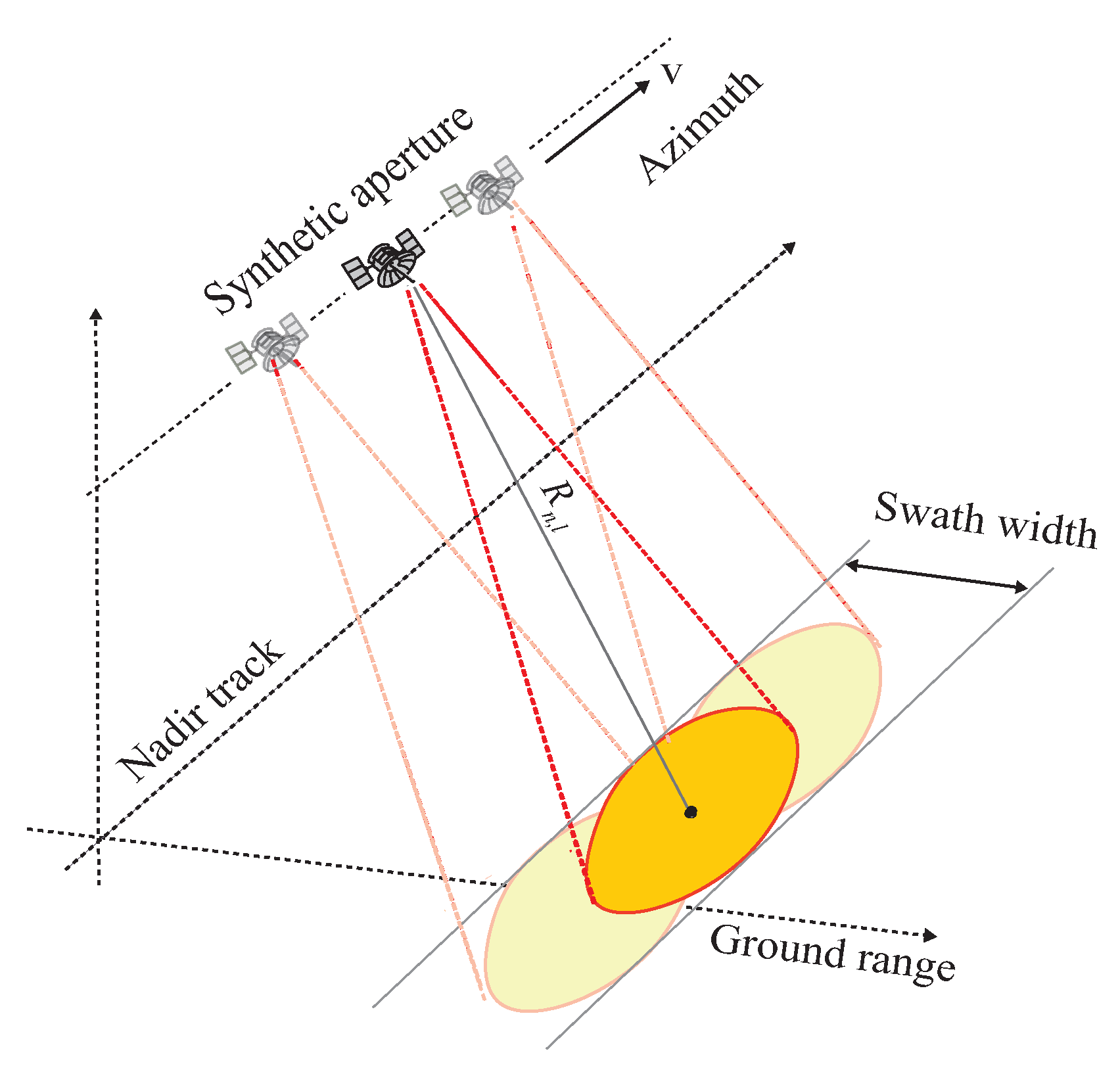
In this section, we give a basic introduction to SAR imaging, and then discuss the sub-Nyquist SAR and associated image formation method.

2.1. SAR Imaging

For simplicity, we take the stripmap SAR as an example. As shown in Figure 2, the radar platform travels along azimuth direction at a constant velocity while the radar illuminates a scene. As the radar moves, the SAR transmits a pulse Re s t e j 2 π f 0 t with carrier frequency f 0 and bandwidth B to illuminate the scene and collect its echo data, and this procedure is sequentially conducted every pulse repetition interval (PRI) T to collect multiple coherent measurements that contains the reflectivity information about the scene. Supposing that the illuminated scene is discretized into K scattering units with predesigned resolution, then the received backscattered signal can be modeled as superpositions of the echo signals due to these scattering units. For the l-th observation, after demodulation, the complex baseband envelope can be expressed as
y l t = n = 1 K D l , n t σ n .
In (5), σ n is the complex reflectivity coefficient of the n-th scattering unit and D l , n t is a waveform related to the scattering unit as
D l , n t = w a l T η n s t 2 R l , n 2 R l , n c c × exp j 4 π f 0 R l , n j 4 π f 0 R l , n c c ,
where w a · is the antenna beam pattern, η n is the beam center crossing time, and R l , n is the slant range of the n-th scattering unit. For subsequent digital processing, the baseband echo (6) is sampled according to the Nyquist theorem to collect its complex sample vector y l with length N r = B T . A coherent combination of N a echo data forms a two-dimensional data matrix of complex samples Y = y 1 , , y N a . Let us denote the reflectivity map of the discretized scene by a complex image matrix X with size K r × K a . By stacking the echo data matrix and image matrix into vectors respectively, we obtain the following observation model
y = D x ,
where y = vec Y is the vectorized Nyquist rate echo data with length N = N r N a , and x = vec X is the image vector with length K = K r K a . The SAR image can be well focused by traditional matched-filter-based focusing methods, x m f = D * y , such as range-Doppler algorithm and chirp scaling algorithm (CSA). A virtue of these algorithms is that they are numerically efficiency with O N log N complexity, owing to range and azimuth decoupled processing and fast Fourier transform (FFT) operations.

2.2. Sub-Nyquist SAR

Since its invention, CS theory has been applied to SAR systems to reduce the data rate and subsequent demands on storage [27,28]. In classical SAR systems, radar echoes are sampled at Nyqusit rate in azimuth and range dimensions, respectively. Therefore, CS can be conducted both in azimuth and range dimensions. In the azimuth dimension, CS is often realized through randomly transmitting a reduced number of pulses at irregular azimuth positions. A shortcoming of this strategy is that the underlying mathematical model falls into the paradigm of block sampling, which limits the performance of its sensing matrix. In the range dimension, CS of the analog radar signals involves structured sampling systems, such as the Xampling system reported in [4,12]. This paper focuses on the sub-Nyquist sampling in range dimension, so the azimuth-dimension CS is not considered. Our work can be naturally extended to the case of azimuth-dimension CS.
In a sub-Nyquist SAR, the sub-Nyquist measurements of the l-th observation can be expressed as
y l c s = Φ l y l + n l , l [ N a ] ,
where y l c s and n l are the length- M r sub-Nyquist measurement vector and the measurement noise vector, respectively, and Φ l is the M r × N r measurement matrix specified by the sampling system for l-th observation. Let us collect the sample vectors to form a 2D measurement Y c s = y 1 c s , , y N a c s , and denote its vectorization by y c s = vec Y c s with length M = M r N a . We can express the sub-Nyquist measurements of (7) as
y c s = A x + n ,
where A = diag Φ 1 , , Φ N a D C M × K is the sensing matrix and n = vec ( [ n 1 , , n N a ] ) C M × 1 is the contaminating measurement noise.
Typically, the measurement dimension M is much smaller than the image size K, and then image formation from the linear system (9) is an ill-posed problem. However, assuming that the image vector x is sparse and the sensing matrix A satisfies the RIP, the image can be estimated by solving the following basis pursuit denoising (BPDN) problem
min x 1 2 A x y c s 2 2 + λ x 1 ,
where λ > 0 is a regularization parameter used to trade off between sparsity and data fidelity. For this optimization problem, the very high dimension of x precludes the direct application of classical optimization methods, such as inner-point methods and greedy algorithms. However, matrix-vector products involving A and its adjoint A * , if they exist, can be used to speed up many popular algorithms for solving (10), such as fast iterative shrinkage-thresholding algorithm (FISTA) [25]. In this sense, the sampling system is expected to have special structures for fast matrix-vector products. Then, the recovery algorithm can be adapted for fast image formation.

3. Quadrature Compressive Sampling for SAR with Independent Measurements

In this section, we present the QuadCS-based sampling system for sub-Nyquist SAR. For sequential SAR observations, we use independent chipping sequences to modulate the echoes; thus, the measurement matrix Φ l is different from one to another. We call this strategy as independent measurements. Then, we provide the frequency-domain representation of this strategy for the convenience of subsequent RIP analysis. As will be shown in Section 5, this strategy will lead to smaller RICs and therefore better recovery performance.

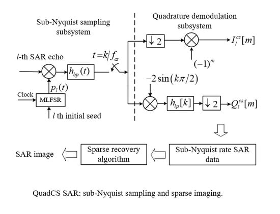
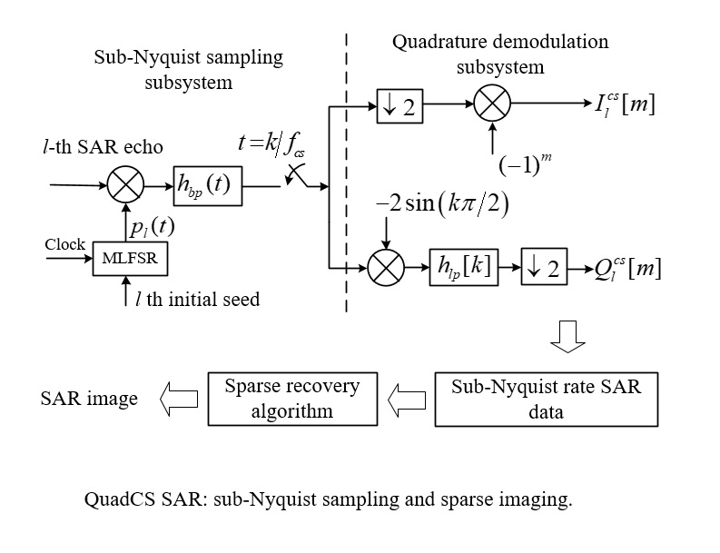
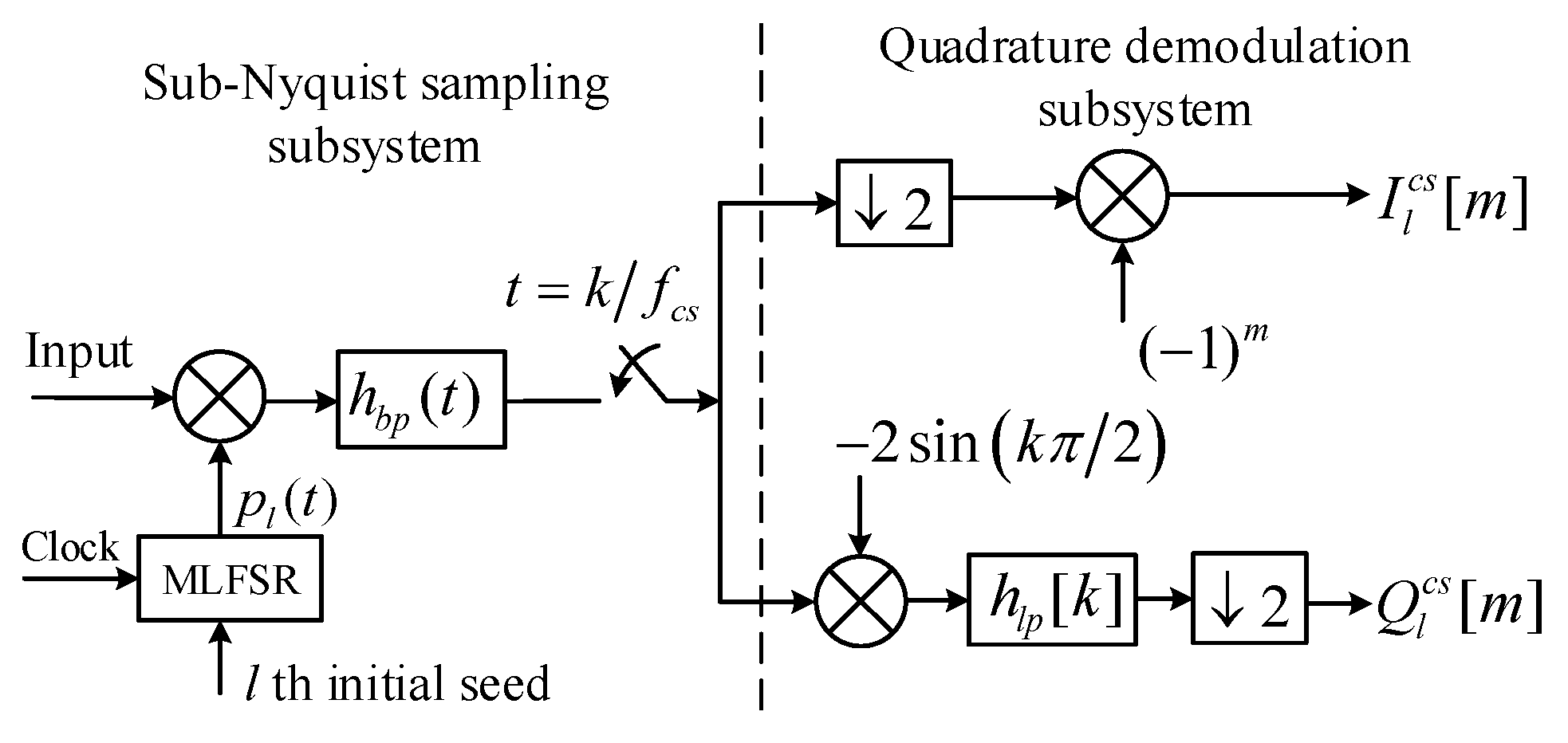
3.1. Sampling SAR Echoes via QuadCS

The fundamentals of the QuadCS system [10] are shown in Figure 1, which consists of two subsystems: a sub-Nyquist sampling subsystem and a digital quadrature demodulation subsystem. Before inputting them into the system, the radar signal is down converted to intermediate frequency (IF) f I . With an IF input signal, the first subsystem generates a compressive bandpass signal and its bandpass samples, and then the second subsystem translates the bandpass samples into the complex baseband samples by quadrature demodulation.
Let us take the l-th observation to illustrate its operating principle. In the first subsystem, the IF radar echo Re y l ( t ) e j 2 π f I t is modulated by a chipping sequence p l t with the bandwidth not less than that of y l t . The mixing operation will spread the frequency content of the baseband signal y l t to full spectrum of p l t . The mixing output is filtered by a bandpass filter h b p t with center frequency f 0 and bandwidth B c s B . The filter outputs the compressive bandpass signal r l ( t ) ,
r l ( t ) = h b p t τ p l τ Re y l ( τ ) e j 2 π f I τ d τ = Re y l c s t e j 2 π f I t ,
where y l c s t is the compressive complex envelope given by
y l c s t = h b p t τ e j 2 π f I ( t τ ) p l τ y l τ d τ ,
with I l c s t = Re y l c s t and Q l c s t = Im y l c s t denoting the compressive I and Q components of y l c s t , respectively. The filter output y l c s t is then sampled by a low-rate ADC to generate a sub-Nyquist sequence y l c s k = r l k / f c s , which is the baseband sample of y l c s ( t ) . The sampling rate f c s is set according to bandpass sampling theorem as f c s = 4 f L + 2 B c s / 4 k + 1 , where f L = f I B c s / 2 and k is a positive integer satisfying k f L / 2 B c s . The second subsystem is to extract digital I and Q sequences from the sub-Nyquist sequence y l c s k . Its operation is the same as classic quadrature sampling [20]. Because of the down-sampling operation, the rate of the digital I and Q sequences, I l c s m = I l c s m T c s and Q l c s m = Q l c s m T c s , is half that of y l c s k , T c s = 2 / f c s . In a PRI, we obtain M r = T / T c s sub-Nyquist complex samples y l c s m = I l c s m + j Q l c s m or 2 M r samples of I and Q components, which is much less than 2 B T by the classical Nyquist sampling.
Although the QuadCS system works on analog bandpass signals, its output y l c s m can be characterized as a linear combination of the sparse coefficient vector x = σ 1 , , σ N T . Inserting (5) and (6) into (12), we have
y l c s t = n = 1 K σ n h b p t τ e j 2 π f I ( t τ ) × p l τ D l , n τ d τ = n = 1 K σ n A l , n t ,
where A l , n t is the compressive signal of D l , n t
A l , n t = h b p t τ e j 2 π f I ( t τ ) p l τ D l , n τ d τ .
Then, the sub-Nyquist complex samples can be expressed as
y l c s m = n = 1 K σ n A l , n m T c s .
To get a standard CS formulation, let us define the sub-Nyquist measurements vector of the l-th observation as
y l c s = y l c s 0 , , y l c s M r 1 T ,
collect all N a observations as Y c s = y 1 c s , y 2 c s , , y N a c s or its vector form y c s = vec Y c s , and define the sensing matrix A as
A m + ( l 1 ) M r , n = A l , n m T c s ,
for m [ M r ] , l [ N a ] and n [ N ] . Then, we have the sub-Nyquist measurements model y c s = Ax as given by (9) in the noisy case. However, the structure of the sensing matrix A here is not as clear as that in (2). To decompose the sensing matrix into an explicit structured form, we next analyze the QuadCS in frequency domain, which is also important for subsequent discussions on the fast imaging algorithm and RIP.

3.2. Frequency-Domain Representation

From (11), we can see that the QuadCS involves a time-domain product and a bandpass filtering operation. The time-domain product is equivalent to frequency-domain convolution, which can be described by the product of a Toeplitz matrix by a vector, and the bandpass filtering can be modelled by a truncation operation in frequency domain under the assumption of idea frequency response. Based on the above-mentioned view, we have the frequency-domain measurement model of QuadCS as studied in [10].
Since each observation interval has a duration T, the chipping sequences p l t can be expressed in Fourier series as
p l ( t ) = i = L p L p ρ i , l e j 2 π f p i t ,
where f p = 1 / T , ρ i , l is the Fourier coefficient of p l t , and L p B T is a positive integer. Denoting the discrete Fourier transform (DFT) of y l c s by y ^ l c s , it can be given by [29]
y ^ l c s = 1 M r T l F r y l ,
where F r is a N r × N r normalized DFT matrix after fftshift (fftshift is to shift zero-frequency component to the center of spectrum), and T l is a M r × N r Toeplitz matrix defined by the Fourier coefficients as
T l = ρ L 0 + N r 1 , l ρ L 0 + N r 2 , l ρ L 0 , l ρ L 0 + N r , l ρ L 0 + N r 1 , l ρ L 0 + 1 , l ρ L 0 , l ρ L 0 1 , l ρ L 0 + M r 1 , l ,
where L 0 = M r + N r 1 . The Toeplitz structure of T l results from the convolution between the spectrums of the chipping sequence and the input signal. Due to bandpass filtering, T l does not contain all Fourier coefficients of p l ( t ) . Next, according to (19), we can describe the time-domain sub-Nyquist measurements as
y l c s = F m * y ^ l c s = 1 M r F m * T l F r y l ,
where F m is a M r × M r normalized DFT matrix after fftshift. Then, the measurement matrix Φ l can be described as
Φ l = 1 M r F m * T l F r ,
which is independent from one observation to another due to the adoption of different chipping sequences. Finally, according to (8) and (9), we can rewrite the sensing matrix as a structured form, A = diag Φ 1 , Φ 2 , , Φ N a D . The first factor of A is a block diagonal matrix with independent diagonal blocks. Therefore, the sensing matrix A has more randomized structures, which better meets the principle of random measurement in CS. In addition, the block diagonal and Toeplitz structures are also helpful for deriving a fast sparse recovery algorithm, as will be shown later.

3.3. Remarks

The QuadCS generates independent measurement matrices while does not complicate hardware implementation. In the system, chipping sequences are realized by a pseudo-random number generator, which can be implemented using a MLFSR. The MLFSR has the benefit of providing a random sequence of ± 1 with zero average, and it offers the ability of regenerating the same sequence by a given initial seed [6]. This technique has been widely used in modern radio communication, such as CDMA. During sequential observations of SAR, the initial seeds are easily assigned to different values, which can be set in advance or in real-time. On the contrary, in the Xampling system [4,12], it is not allowed to generate varied measurement matrices among different observations, because four bandpass filters with different passbands are utilized to perform sub-Nyquist measurement and the measurement matrix is inherently fixed when the hardware is built. Moreover, bandpass filters cannot sample SAR echoes randomly enough in frequency domain and thus often generate bad sensing matrices, as observed in the following simulations. As for non-uniform sampling, it often imposes strict timing requirements on the digital circuits to preserve timing information [8,30], which makes it difficult to interface with synchronous digital circuits. In fact, it is easier to build a high-rate modulator via mixer/chipping sequence combination than a specially designed non-uniform sampler [31].

4. Fast Sparse Imaging with QuadCS Measurements

As a standard sparse recovery problem in CS, we model our imaging problem as the BPDN formulation in (10). For the large-scale problem, the very high dimensions of A often precludes the direct application of off-the-shelf optimization methods because of two limitations: the matrix A cannot be stored explicitly, and the matrix-vector products involving A and its adjoint A * cannot be quickly calculated. If these two limitations are well resolved, several popular solvers can be used to solve (10), such as FISTA [32], SpaRSA [33], TFOCS [26] and L1LS [22]. In the proposed sampling system, we exploit the block and Toeplitz structure of the sensing matrix A and decompose the matrix-vector products into several fast operations. Then, the matrix A does not need to be stored explicitly, and the matrix-vector products can be fast calculated. By inserting the decomposition into above-mentioned solvers, we derive a FISTA-based fast SAR imaging algorithm for the proposed sub-Nyquist SAR system, and analyze the algorithm complexity.

4.1. Fast Matrix-Vector Products

As we have discussed, the sensing matrix A = Φ D consists of two parts: measurement matrix Φ and basis matrix D . To obtain the desired fast matrix-vector products for A and A * , we are going to exploit the inner structures of the two matrices. The following content is to expand the derivations in detail.
Let us first discuss the Toeplitz structure as shown in the frequency-domain model (21). Since  T l is a Toeplitz matrix, it can be viewed as a submatrix of a 2 L 0 + 1 × 2 L 0 + 1 circulant matrix C l defined as
C l = ρ L 0 , l ρ L 0 1 , l ρ L 0 , l ρ L 0 , l ρ L 0 , l ρ L 0 + 1 , l ρ L 0 1 , l ρ L 0 , l ρ L 0 , l .
Specifically, T l is exactly the right N r columns and top M r rows of C l . Let us define row and column truncation matrices as
Δ r = I M r 0 N r 1 ,
and
Δ a = 0 M r 1 I N r ,
respectively. Then, we embed T l into C l as follows:
T l = Δ r C l Δ a .
Since circulant matrices can be diagonalized by DFT matrices, there exist fast matrix-vector products for circulant matrices via FFT and the computational complexity is O ( N log ( N ) ) . The goal of (26) is to extend this property to the Toeplitz matrix T l . Specifically, let us define an integer L = 2 L 0 + 1 , and a vector ρ l = ρ L 0 , l , ρ L 0 , l , , ρ L 0 1 , l T which is the first column vector of C l , and denote the L × L DFT matrix as F L . Then, the circulant matrix C l can be diagonalized as
C l = F L diag L θ l F L * ,
where θ l = F L ρ l . Inserting (26) and (27) into (21), we have
y l c s = L M r F m * Δ r F L diag θ l F L * Δ a F r y l .
Defining Θ = θ 1 , , θ N a , then the 2D QuadCS measurement Y c s can be written as
Y c s = L M r F m * Δ r F L Θ F L * Δ a F r Y ,
which mainly involves FFTs and thus has a low complexity. Note that, from (29), we find that the random matrix Θ performs “Hadamard scrambling” to inject randomness into the measurements.
Next, we analyze the inner structure of the basis matrix D . It has been suggested that conventional imaging algorithms, such as CSA, can be exploited to derive its fast matrix-vector product for D [5,34], which demonstrate that the matrix is also highly structured. We assume that the SAR operates in stripmap mode and the transmitted pulses are linear frequency modulated (LFM); then, CSA can be used to obtain the SAR image, which can be described in a compact form as
X C S A = H 3 F r * H 2 F r H 1 Y F a F a * .
In this equation, X C S A is the SAR image output by CSA, H 1 , H 2 , H 3 are phase compensation matrices (i.e., their entries lie in the unit circle in C , for more details, cf. chapter 6 in [35]), and F r , F a are the range and azimuth DFT matrices, respectively. Because CSA is a high precision algorithm, X C S A is a valid approximation of the reflectivity map X . For ease of discussion, we omit the approximation error, i.e., we take X = X C S A , and in this sense, X and Y have the same size, i.e., K r = N r and K a = N a . After simple derivation, the inversion of (30) is given by [5]
Y = H ¯ 1 F r * H ¯ 2 F r H ¯ 3 X F a F a * .
It is easy to see that the linear system (31) is equivalent to y = D x with proper reshape operations. Furthermore, since the involved FFTs and Hadamard products in (30) and (31) are unitary operators, the matrix D is also unitary [5].

4.2. FISTA-Based Fast Imaging Algorithm

FISTA is an accelerated variant of the iterative shrinkage-thresholding algorithms (ISTA), and it has a quadratic rate of convergence thanks to the generalized Nesterov’s method [23,25]. Each iteration of FISTA involves matrix-vector product involving A and its adjoint A * followed by a shrinkage/soft-threshold step as follows:
x k + 1 = T λ / L f z k A * A z k y c s / L f ,
where x k + 1 , z k are iterative variables, L f is the Lipschitz constant for the gradient Δ f of the function f x = A x y c s 2 2 , and T λ / L f · is the soft shrinkage operator defined as
T τ x i = x i τ x x i , x i > τ ; 0 , otherwise .
From (32), we know that the matrix-vector products involving A and its adjoint A * dominate the computational cost in each iteration. The previous subsection shows that the matrix-vector products can be fast calculated through matrix decomposition. Now, we merge this calculation strategy into FISTA and thus provide a FISTA-based fast imaging algorithm, as shown in Algorithm 1.
Algorithm 1: Fast sparse imaging with QuadCS measurements
Input:
 Operators M , D and their adjoints; QuadCS measurement Y c s ; number of iterations N i t e r ; λ ;
Output:
 Sparse SAR image X # ;
1:
initial: take λ , L f R , Z 0 = X 0 = 0 , q 0 = 1 , k = 1 ;
2:
repeat
3:
Z k = Z k 1 1 L f D * M * MD Z k 1 Y c s ;
4:
X k = T λ / L f Z k ;
5:
q k = 1 2 + 1 2 1 + 4 q k 1 2 ;
6:
Z k = X k + q k 1 1 q k ( X k X k 1 ) ;
7:
k = k + 1 ;
8:
until k N i t e r ;
9:
return X # = X k 1 ;
For ease of description, we denote the right sides of (29) and (31) by operators as M Y and D X , respectively, and denote vec ( · ) by an operator V . With these notations, we can express the matrix-vector product of A as
Ax = V MD V * x .
Similarly, the matrix-vector product of the adjoint A * is given by
A * y c s = V M * D * V * y c s ,
where the adjoint operator D * is given by the operations on the right side of (30) and M * is given by
M * Y c s = L M r F r * Δ a T F L Θ ¯ F L * Δ r T F m Y c s .
It is clear that the involved operations in the right sides of (34) and (35) mainly consist of FFTs and Hadamard products. Therefore, we can conclude that A and its adjoint A * both admit fast matrix-vector products.

4.3. Complexity

Without fast matrix-vector products for A and A * , we need to store the M × N matrix A explicitly and compute the involved matrix-vector products directly. For a small scene of 1024 × 1024 pixels and compression ratio M / N = 1 / 8 , it requires 1024 GB to store the matrix A with double precision, and roughly 1.3744 × 10 11 complex multiplications to compute the matrix-vector product Ax . Obviously, the image recovery will be numerically intractable. With the fast matrix-vector multiplications (34) and (35), we only need to store N r × N a matrices H 1 , H 2 , H 3 and Θ . It only requires 32 MB to store the four matrices and roughly 8.2 × 10 4 complex multiplications to compute Ax for a scene of 1024 × 1024 size, which are significantly smaller than the previous requirements. In general, the storage cost is reduced form O ( M N ) to O ( N ) , and the computational cost is reduced from O ( M N ) to O ( N log ( N ) ) per iteration, respectively.
Looking back to the traditional imaging algorithm, CSA, it only needs to evaluate (30) once to form a SAR image. Specifically, it involves 2 N r N a log N r + log N a + 3 N r N a complex products, or in a compact form, O N log N complexity. The proposed iterative algorithm exhausts more overhead compared to CSA, depending on the number of iterations. Indeed, the essence of CS is to sacrifice the computational cost in return for the reduction of sampling/data rate.

5. Restricted Isometry Property (RIP) Analysis
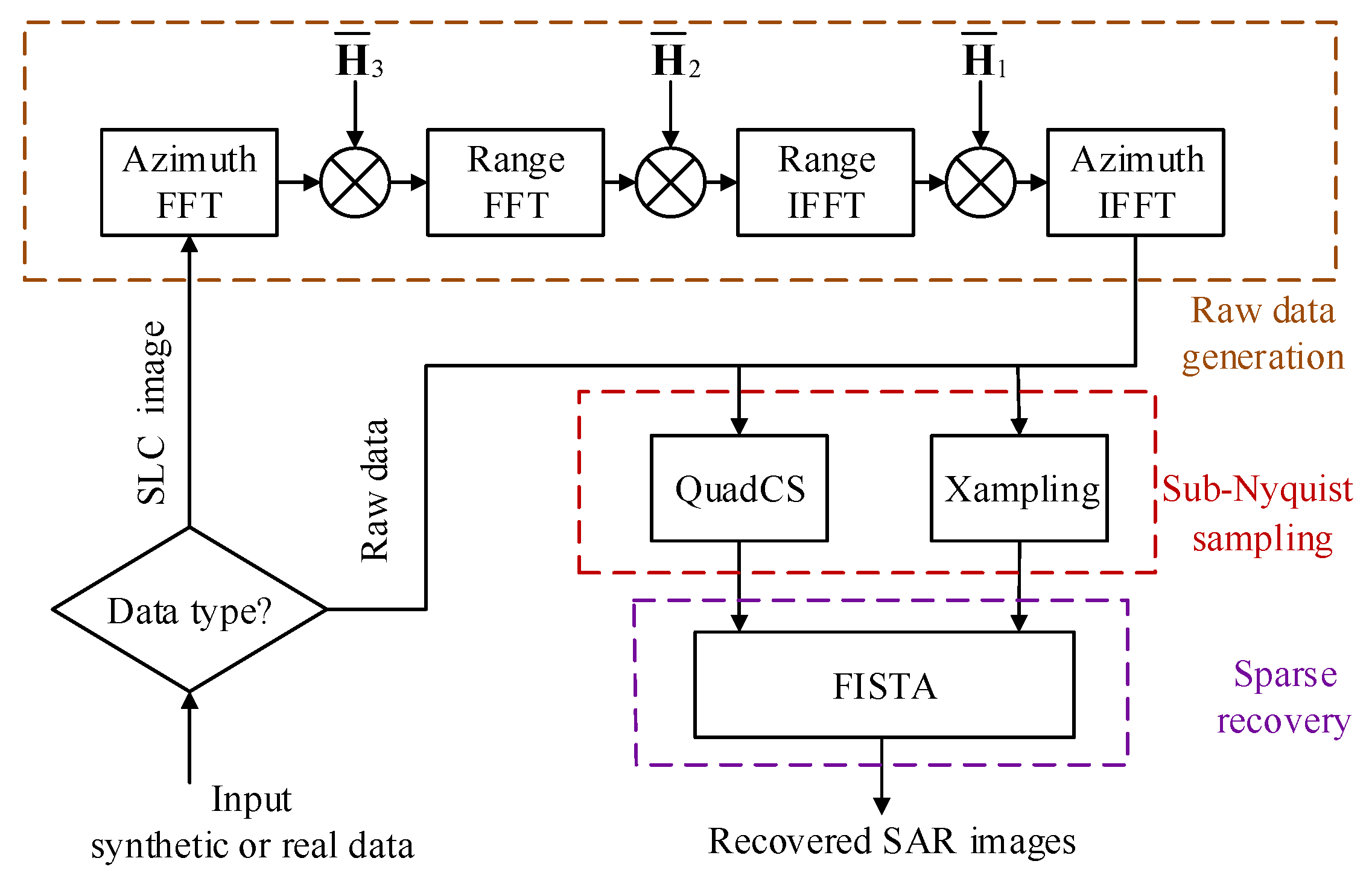
In this section, we derive the RIP of the sensing matrix A resulting from the proposed sampling system. The established RIP condition shows that the strategy of independent measurements provides a “diversity gain”, which is up to N a . Therefore, the sensing matrix A has smaller RICs with independent measurements compared to that with fixed measurements (i.e., with equal chipping sequences), and thus leads to lower sampling/data rate and smaller recovery error.
Our derivation is based on the concentration of measure (CoM) inequality [36], which is one of the leading techniques for the RIP analysis of random sensing matrices in CS. The CoM inequalities have been established for the random matrix with i.i.d. entries and other structured matrices. However, these results are not applicable to the proposed sensing matrix A because of its special factornizatio. In the following, we first derive a CoM inequality of the matrix A , and then establish a RIP condition on it. The CoM inequality of A is formulated in Lemma 1.
Lemma 1.
Let x be a s-sparse vector in C N . For an arbitrary 0 < δ < 1 , we have
P A x 2 2 x 2 2 δ x 2 2 4 exp δ ξ ϖ 2 M 16 χ s ,
where M is the number of sub-Nyquist measurements, χ denotes two settings of chipping sequences and is defined as
χ = 1 , independent chipping sequences , N a , equal chipping sequences .
ξ is the duty cycle of radar transmitted signals, and ϖ is the maximum value of the normalized antenna beam pattern defined as
ϖ = w a 0 T a T a T a 2 2 T a T a 2 2 w a 2 η d η ,
where T a is the antenna footprint time.
Proof. 
The proof is given in Appendix A.1. □
Lemma 1 points out that, with independent measurements, the probabilistic tail bounds of the CoM decays exponentially N a times faster than that with fixed measurements. Since the CoM inequalities quantify how well a random matrix preserve the norm of a high-dimensional signal in the mapped low-dimensional space [37], the independent measurements result in a better distance-preserving property for the sensing matrix A , which is the essence of RIP.
Based on the CoM inequality in Lemma 1, we can derive a uniform tail bound of A S * A S I s 2 for a fixed subset S [ N ] with card S = s using the covering number estimate [38]. Then, we take the union bound over all subsets S [ N ] of cardinality s, to derive the following RIP condition.
Theorem 1.
The restricted isometry constant δ s of the sensing matrix A satisfies δ s < δ for some constant 0 < δ < 1 with probability exceeding 1 η provided that
M 32 χ s δ ξ ϖ 2 s ln e N s + 4 s ln 3 + ln η 4 .
Proof. 
The proof is given in Appendix A.2.□
Theorem 1 gives the RIP condition on the sensing matrix A . The key parameters in (40) are M and χ , which describe the measurement amount and the setting of chipping sequences, respectively. If M (or equivalently, compression ratio) is properly chosen according to the sparsity s and the imaged scene size N, the sensing matrix A will satisfy RIP with high probability in both settings of chipping sequences. However, the measurement amounts required by the two settings vary somewhat surprisingly, up to a multiplicative factor N a . This variance suggests that the strategy of independent measurements provides a diversity gain, which is similar to the waveform diversity gain in MIMO radar. For a given imaged scene, the diversity gain results in lower sampling/data rates. On the other hand, the parameters ξ and ϖ are often fixed in a given SAR operation mode, and they suggest that the duty cycle and the antenna beam pattern have a direct influence on the RIP. Intuitively, for smaller ξ or ϖ , each column of the basis D will be localized in smaller regions, which is bad for the sensing matrix.
Another benefit of the diversity gain is that, with the same number of measurements, the RIC is expected to be much smaller, as stated in the following corollary.
Corollary 1.
Let δ s and γ s be the s-order RICs of the sensing matrices for the setting of equal and independent chipping sequences, respectively. For fixed M and η, the RICs satisfy δ s < δ and γ s < δ / N a simultaneously for some constant 0 < δ < 1 with probability exceeding 1 η .
Replacing δ s by δ s / χ in Theorem 1 will prove the corollary. According to CS theory, smaller RIC means smaller recovery error. Thus, independent measurements have better performance than fixed measurements, as revealed by Theorem 2.
Theorem 2.
For a fixed number of measurements M and a fixed probabilistic guarantee 1 η , let s 1 and s 2 be the maximum integers that satisfy δ 2 s 1 < δ # and γ 2 s 2 < δ # with equal and independent chipping sequences, respectively, where δ # = 2 1 . Let x 1 # and x 2 # be the solutions of the constrained BPDN problem
min x x 1 subject to A x y c s ϵ
in the two settings of chipping sequences (38), respectively, then
x x 2 # 2 C 1 σ s 2 ( x ) 1 s 2 + C 2 ϵ C 1 σ N a s 1 ( x ) 1 N a s 1 + C 2 ϵ < C 1 σ s 1 ( x ) s 1 + C 2 ϵ ,
where the last line is exactly the error bound of x x 1 # 2 .
Proof. 
The proof is shown in Appendix A.3. □
Theorem 2 makes a comparison between the recovery error bounds about the two settings of chipping sequences. In (42), the error bound consists of two parts: one is the best s-term approximation error and the other comes from the measurement noise. As shown in Appendix A.3, we have a gain factor s 2 / s 1 N a , which results in much lower best s-term approximation error as shown in (42). Therefore, we can recover more sparse targets in the case of high signal-to-noise ratio (SNR). For example, when N a = 4096 , the gain factor will be 64. Thus, the stability of image recovery is significantly improved provided that the scene is not reasonable sparse. When the SNR decreases, the noisy contribution C 2 ϵ gradually dominates the error bounds, and consequently, the relative errors get closer. Namely, the advantage of QuadCS with independent measurement is weakened in this case. However, there is no doubt that x 2 # always has a smaller recovery error than x 1 # . Note that we recover images by solving (10) instead of (41). In fact, the two problems are equivalent. If x # is a minimizer of the (41) with some ϵ > 0 , there necessarily exists λ 0 such that x # is a minimizer of (10) [39,40]. It should be pointed out that ϵ is related to the noise level and the optimal choice of λ is related to x # and ϵ . In this paper, we assume that the noise level is known for (41), and λ is empirically chosen in (10) according to the noise level. In real SAR applications, the noise level can be measured when no SAR echo arrives at the radar receiver. In future works, we will consider how to deal with unknown noise level adaptively.
In summary, the above theoretical analysis shows that, using independent measurements, the proposed sampling system has smaller recovery error and enables lower sampling/data rate. This conclusion is of great importance since our goal is to achieve low-rate sampling and meanwhile provide robust recovery performance for sub-Nyquist SAR.

6. Simulations

In this section, we conduct several simulations to evaluate the proposed QuadCS-based SAR imaging performance. Results on both synthetic data and real SAR data collected by TerraSAR-X and RADARSAT-1 missions are presented. Comparisons are made between Xampling and QuadCS with equal or independent chipping sequences. The relative error, x x # 2 / x 2 , and the relative root-mean-square error (RRMSE), E x x # 2 / x 2 , are used as the imaging performance metrics.
The simulation scheme is shown in Figure 3 and main radar parameters are summarized in Table 1. Given a synthetic image, real SAR single-look complex (SLC) image (as shown in Figure 4) or a raw data matrix, we use the operations (29) or (34) to generate sub-Nyquist measurements. Similar methods for SAR raw data generation can be found in [41,42]. To model the measurement noise, an additive white Gaussian noise (AWGN) is added. The regularization parameter and the maximum number of iterations are empirically set to 10 3 and 200, respectively. For visualization, the recovered images are mapped to grayscale images by the following map
x i g r a y = | x i | / τ , | x i | τ ; 1 , else ,
where τ is a threshold for preventing the image from being almost black due to the presence of strong scattering points. A default value provided by a SAR image processing toolbox (code “plotimage_sar.m” in PPB toolbox [43]) is adopted in our simulations, which is given by the sum of mean and triple standard deviation of the amplitude image. For ease of description, we refer to QuadCS-IndSeq and QuadCS-EquSeq as QuadCS with independent and equal chipping sequences, respectively, and denote the compression ratio M/N by α .

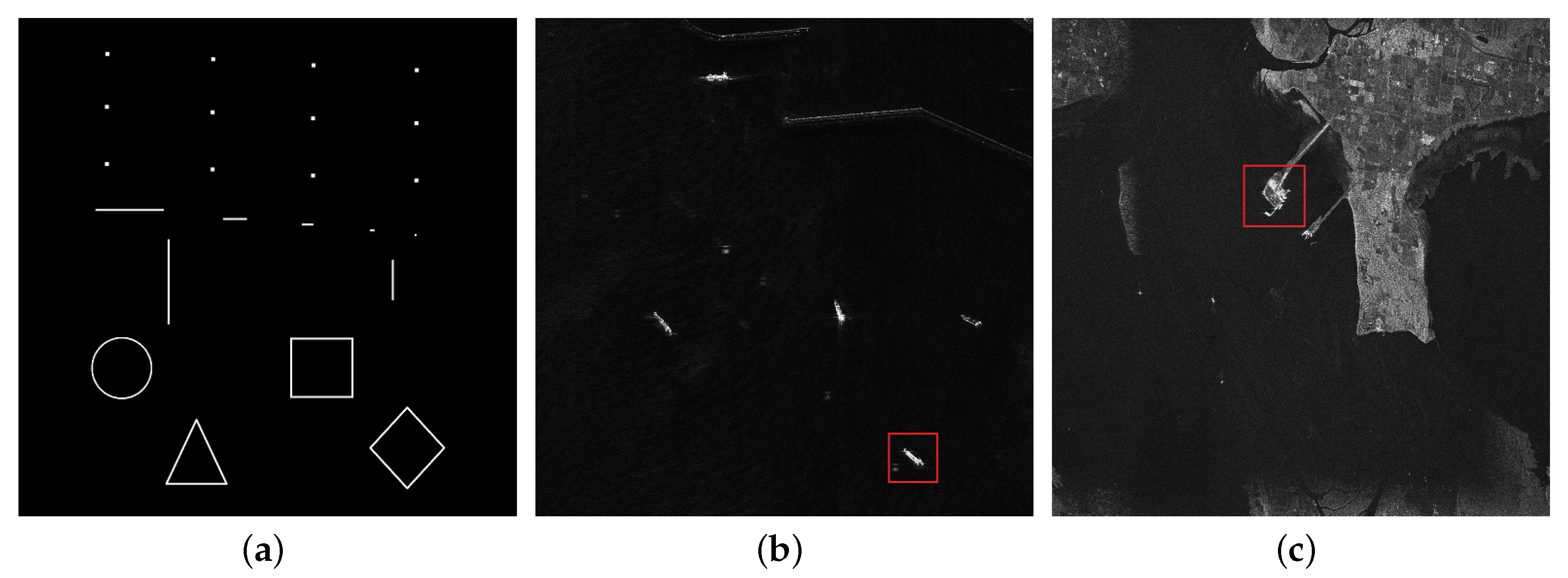
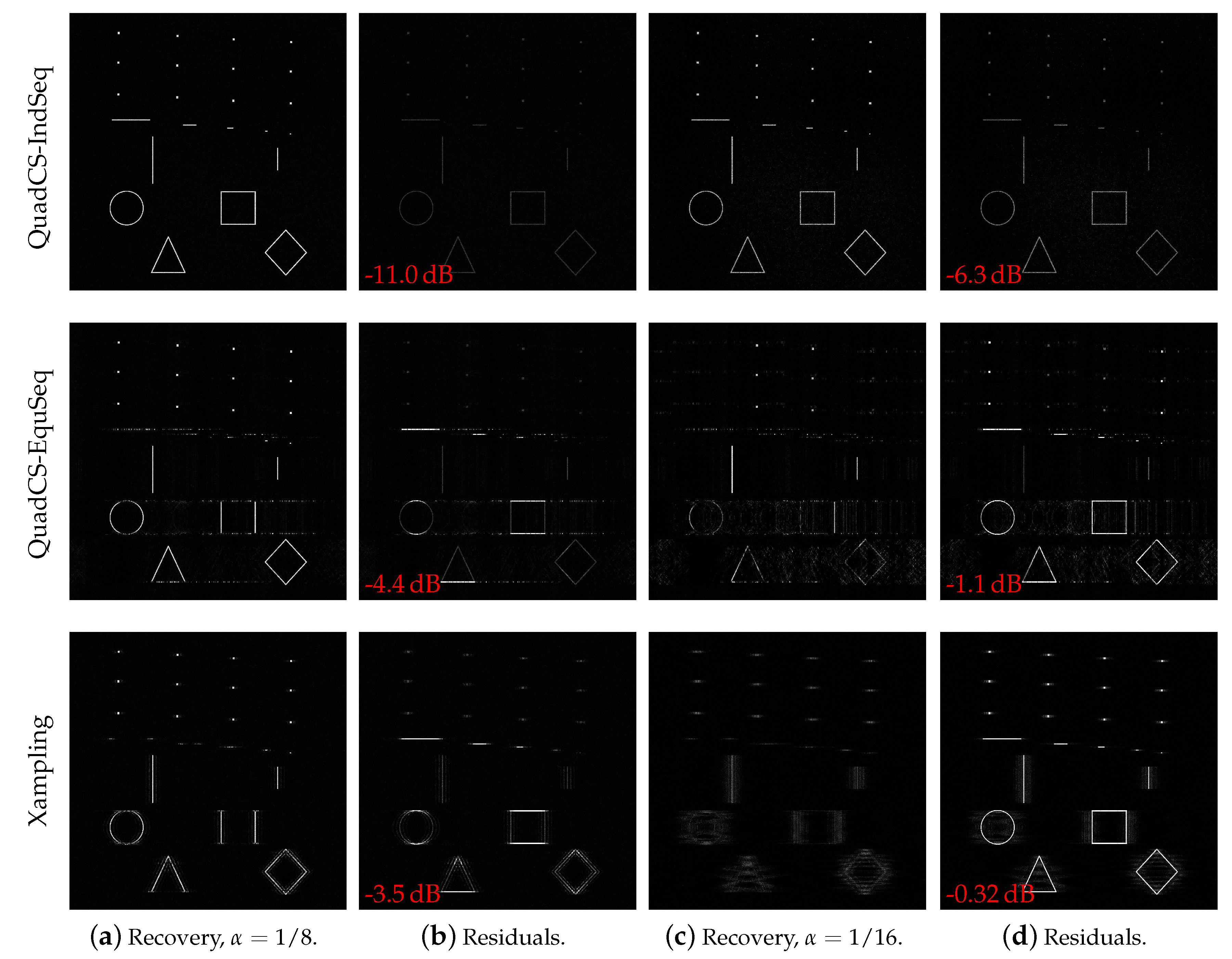
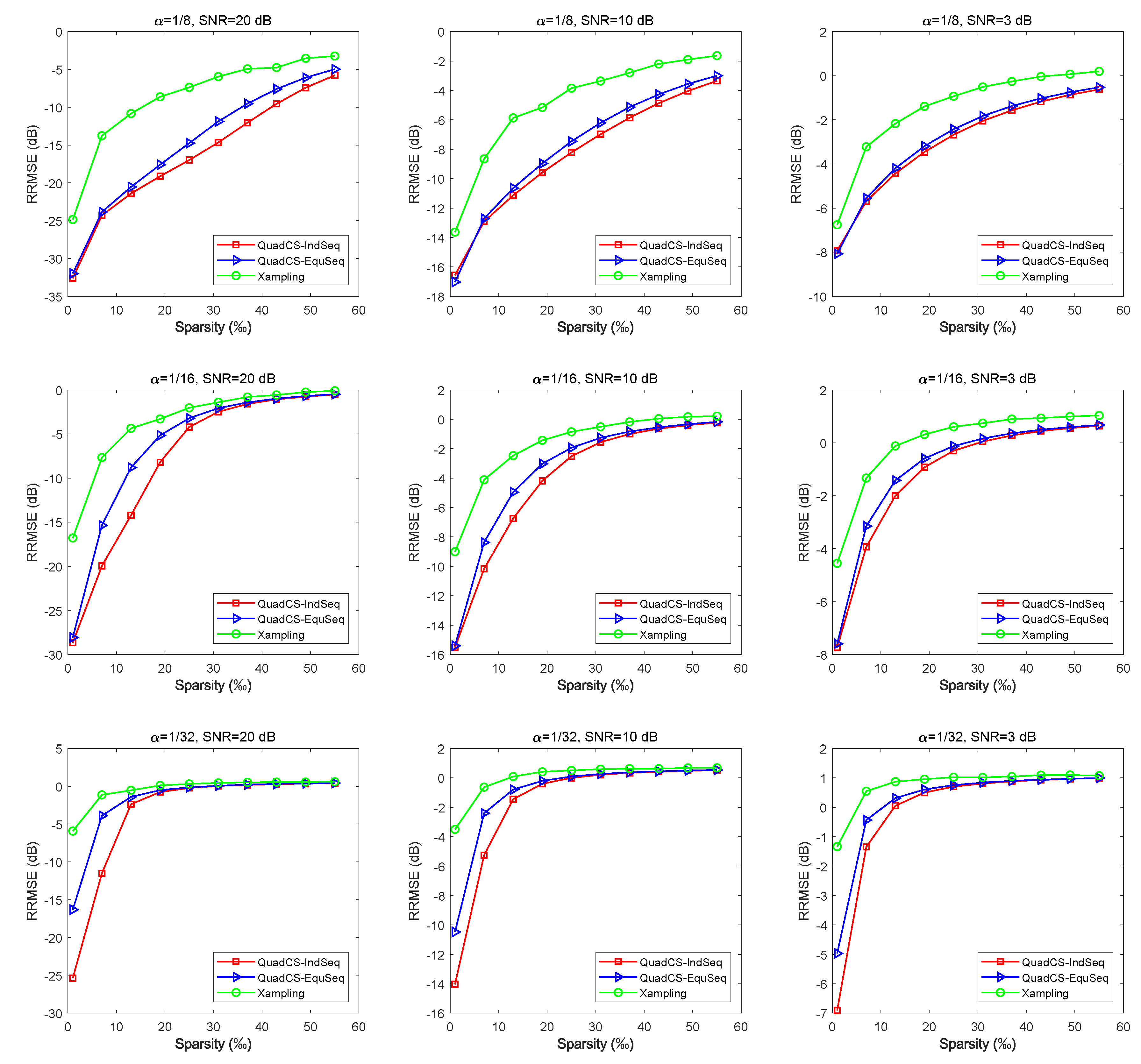
6.1. Simulations with Synthetic Data

Firstly, we use some synthetic geometries as a SLC image, as shown in Figure 4a, to evaluate the imaging performance. The compression ratio is set to 1 / 8 and 1 / 16 , respectively, and the SNR equals 10 dB. As shown in the first column of Figure 5, QuadCS-IndSeq recovers these geometries very well, while QuadCS-EquSeq and Xampling cannot reconstruct horizontal lines clearly. Namely, QuadCS-EquSeq and Xampling cannot recover images in range dimension because of low sampling rate and the usage of fixed measurement matrix in each observation. At the smaller compression ratio 1 / 16 , QuadCS-IndSeq can still recover all geometries with some performance loss, but QuadCS-EquSeq and Xampling cannot reconstruct the geometries correctly. Obviously, the proposed sampling system has the best performance.
Next, we investigate the relationship between RRMSE and the image sparsity under different compressive ratios and SNRs. We choose random subsets of the test image and set its entries to be i.i.d. random variables obeying uniform distribution on [ 0 , 1 ] . The image recovery conducts 100 times and the resulting RRMSE curves are shown in Figure 6. All the figures show that, as the sparsity increases, the recovery errors of all sampling schemes increases. This can be explained by (4) that the best s-term approximation error increases as the sparsity increases. On the other hand, the figures also show that QuadCS-IndSeq has the lowest recovery error in all simulation cases. This is because QuadCS-IndSeq has better RIP, as disclosed in Theorem 2. Furthermore, QuadCS is superior to Xampling in all cases, no matter what the independent measurement strategy is utilized. The reason is that Xampling conducts frequency-domain random sampling by several bandpass filters, so that the randomness is not enough and thus the RIP of corresponding sensing matrix is not very well. Hence, QuadCS is superior to Xampling for sub-Nyqusit SAR.
According to each row subfigures, we find that QuadCS-IndSeq has more performance advantages in the high SNR case (SNR = 20 dB), since the RMMSE relies on the best s-term approximation error in this case. Specifically, as seen from the middle left subfigure in Figure 6, where SNR is 20 dB and compression ratio is 1 / 16 , when the sparsity is 13‰, the RRMSE of QuadCS-IndSeq is about 14.2 dB, while those of QuadCS-EquSeq and Xampling are about 8.8 dB and 4.4 dB, respectively. On the other hand, according to each column subfigure, we know that the image recovery performance degrades faster with the lower compressive ratio, which is the inherent characteristic of sub-Nyquist sampling systems. However, QuadCS-IndSeq still has the best image recovery performance. In summary, our sampling system considerably improves the imaging performance under relatively large sparsity and low sampling rate. However, with the decrease of SNR, the recovery errors mainly come from the noise, as shown in (42); then, the improved performance is gradually diluted.

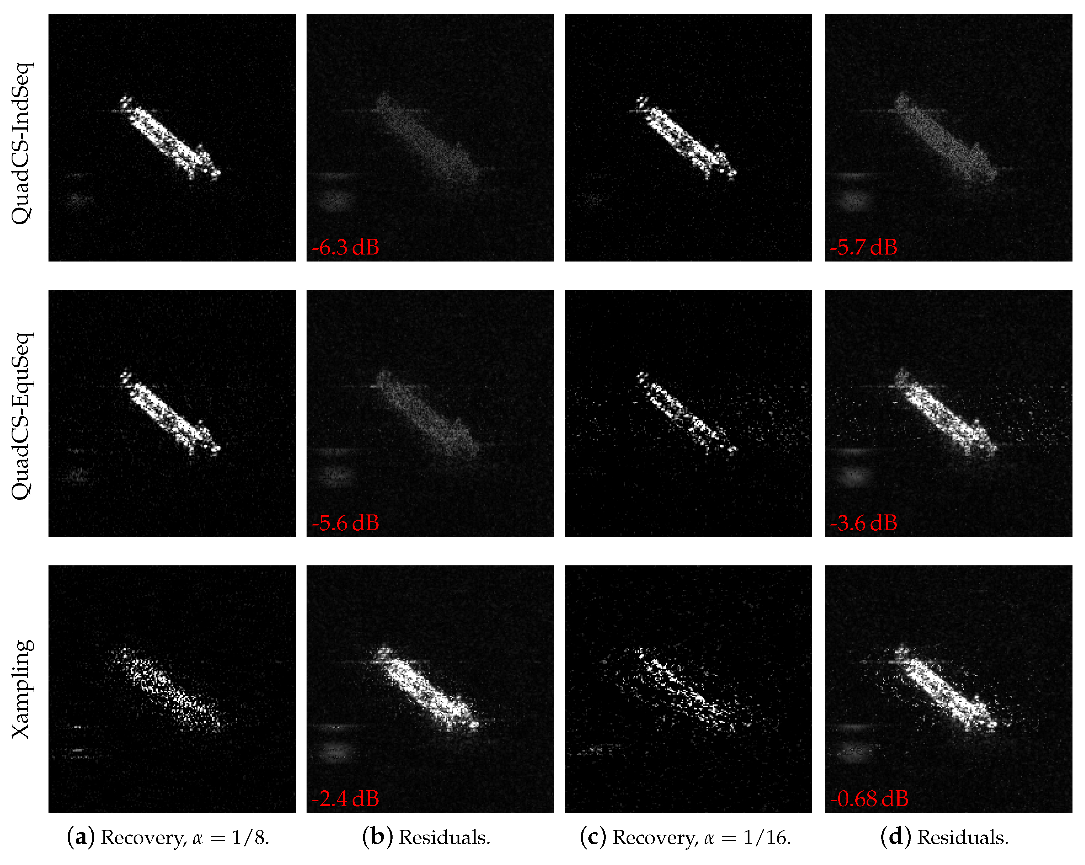
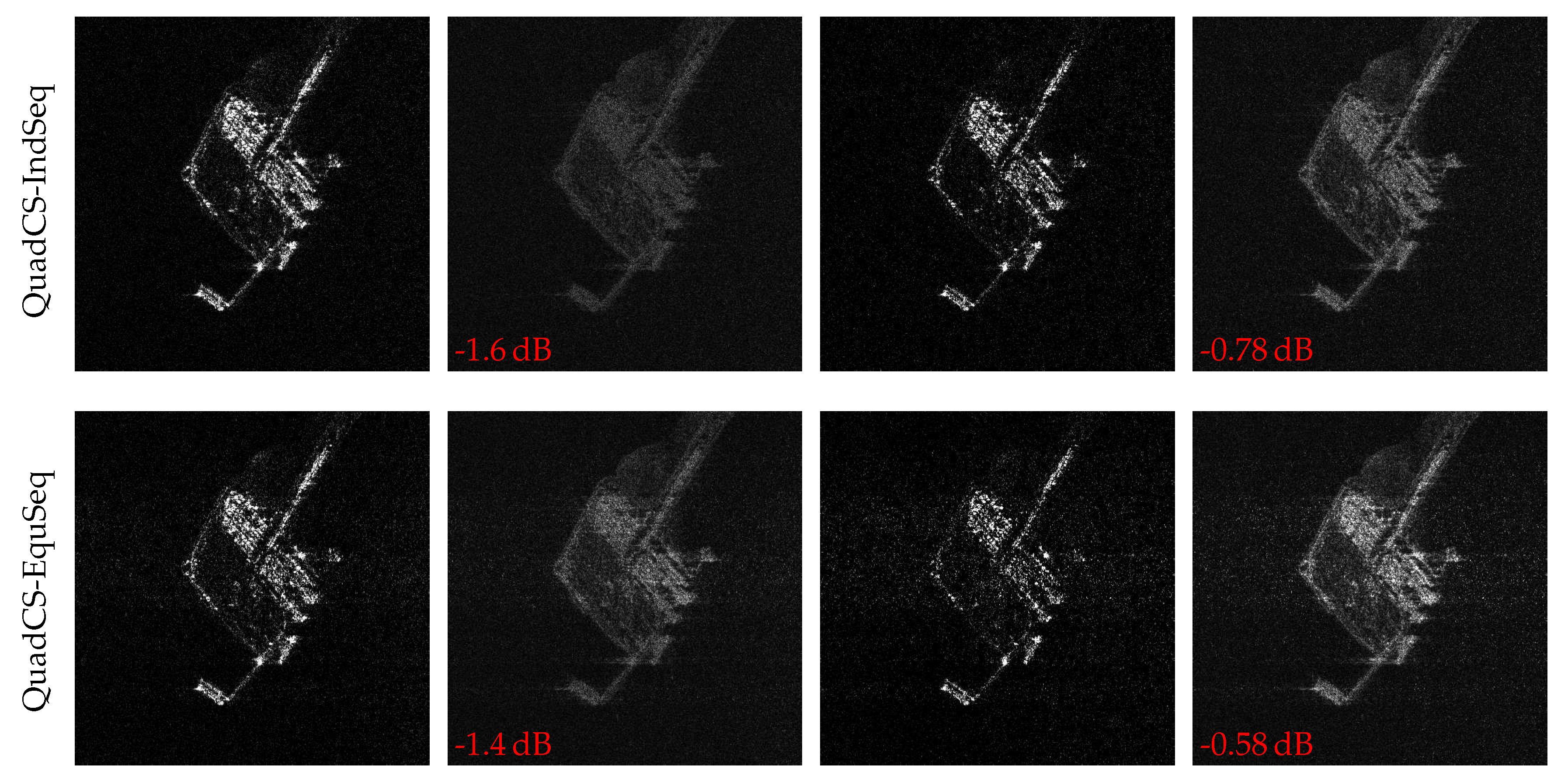
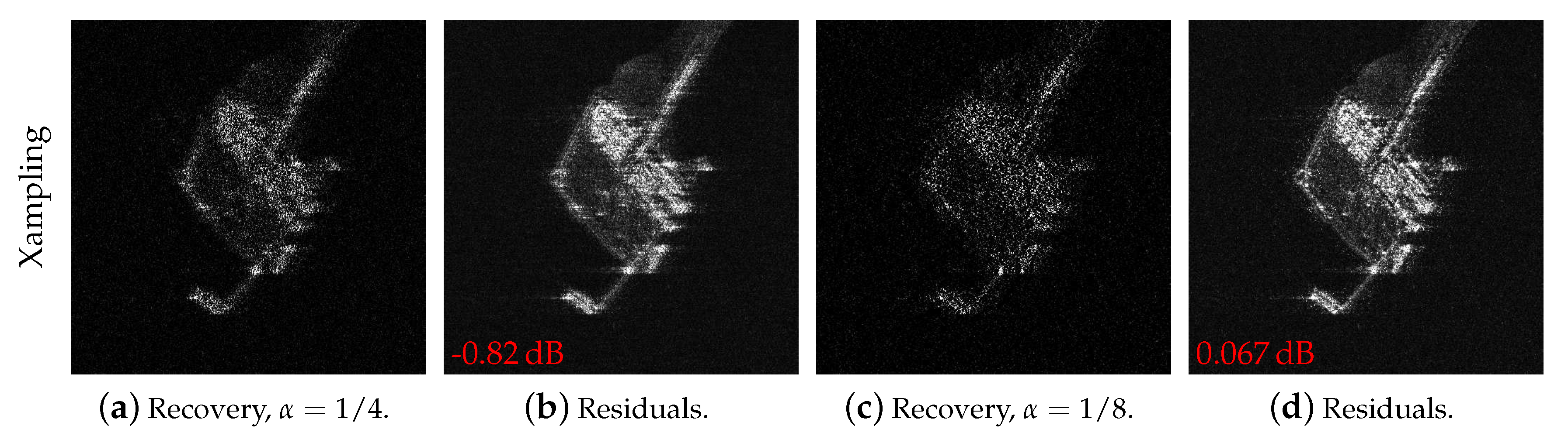
6.2. Simulations with Real SAR Data

Now, we use a real SLC image, shown in Figure 4b, to evaluate the proposed sampling system. The image with size 2048 × 2048 is collected by TerraSAR-X on 4 July 2008, which contains several ships near the coast of Barcelona. For a clear display, we show 200 × 200 area of the recovered images in Figure 7. We find that QuadCS-IndSeq has a smaller recovery error than QuadCS-EquSeq and Xampling.
We also use RADARSAT-1 raw data collected on 16 June 2002 to evaluate the proposed system. Imaging results using the raw data is shown in Figure 4c. Because the scene is not reasonably sparse, we consider larger settings of compression ratios, namely, 1 / 4 and 1 / 8 , respectively. Figure 8 shows a 500 × 500 area of the recovered images. As we noted in Section 1, the recovery error greatly depends on the sparsity of the image. Due to lack of sparsity, the recovery errors are large for all simulated schemes as shown in Figure 8. However, QuadCS-IndSeq still has the lowest recovery errors.

7. Conclusions

In this paper, we presented an efficient sampling system for sub-Nyquist acquisition of SAR data. The proposed system is based on the QuadCS, which is easy to insert randomness into the sensing matrix. With independent measurements in each observation, our system has more randomness than that with fixed measurements in all observations, and thus the corresponding sensing matrix has better image recovery performance. Based on the RIP analysis, we showed that the proposed system has smaller RIC, which can lead to lower sampling/data rate and smaller recover error.
Next, we provided a fast image formation method. Through the frequency-domain representation, we found that the sensing matrix is a block and Toeplitz matrix and its matrix-vector products can be decomposed into several fast operators. In virtue of matrix decomposition, we established a first-order fast SAR imaging algorithm, whose storage and computational complexity are much less than that of the off-the-shelf recovery methods. By using both synthetic data and real data, we made comparisons among QuadCS with independent measurements, QuadCS with fixed measurements, and Xampling. Numerical results showed that the QuadCS with independent measurements achieves much better image qualities than the other simulated schemes.

Author Contributions

H.Y. conceived the research topic, and performed model building, theoretical analysis, numerical simulations and manuscript writing. C.C. assisted with manuscript writing and simulations analysis. S.C. supervised H.Y., provided the reviews and revised the manuscript. F.X. provided the reviews and funding acquisition. All co-authors helped the manuscript writing.

Funding

This work was supported in part by the National Natural Science Foundation of China under grants 61671245, 61571228.

Conflicts of Interest

The authors declare no conflict of interest. The funders had no role in the design of the study; in the collection, analysis, or interpretation of data; in the writing of the manuscript, or in the decision to publish the results.

Abbreviations

The following abbreviations are used in this manuscript:
SARSynthetic aperture radar
RIPRestricted isometry property
CSCompressive sensing
ADCAnalog-to-digital converter
MLFSRMaximal-length linear feedback shift register
FFTFast Fourier transform
PRIPulse repetition interval
CSAChirp scaling algorithm
IFIntermediate frequency
DFTDiscrete Fourier transform
FISTAFast iterative shrinkage-thresholding algorithm
BPDNBasis pursuit denoising
RRMSERelative root-mean-square error

Appendix A

Appendix A.1.

We use the tail bound on Lipschitz functions of i.i.d. random variables to derive the CoM inequality.
Firstly, we describe A x 2 as a Lipschitz function. Let us decompose the vector θ l in (27) as follows:
θ l = F L ρ l = F L S 1 F L p l = J p l ,
where p l is the discrete binary samples of p l t , S 1 circularly shifts the elements of F L p l from top to bottom by one position, and J = F L S 1 F L . In (A1), the Fourier coefficient ρ l is represented by the DFT of the length-L sequence p l . The decomposition (A1) is to represent θ l by the random Bernoulli sequence p l . Let us define
U = F L * Δ a F r Y ,
we can rewrite (29) as
Y c s = L M r F m * Δ r F L Θ U .
Define a matrix
Γ = L M r I N a F m * Δ r F L diag Θ ,
and denote u = vec U ; then, (A3) can be written in a matrix-vector multiplication form as
y c s = A x = Γ u ,
where u = I N a F L * Δ a F r D x . In the following, we replace A x 2 by Γ u 2 for the convenience of proof. With the equivalence between (A3) and (A5), Γ u 2 2 can be represented as
Γ u 2 2 = L M r F m * Δ r F L Θ U F 2 = L M r l F m * Δ r F L diag u l θ l 2 2 = L M r l F m * Δ r F L diag u l F L * F L J p l 2 2 = L M r Δ ^ R F ^ L J ^ p 2 2 ,
where
p = vec ( P ) ,
Δ ^ = I N a Δ r ,
F ^ L = I N a F L ,
J ^ = I N a J ,
R = diag F L diag u 1 F L * , , F L diag u N a F L * = F ^ L diag U F ^ L * .
P = p 1 , p 2 , , p N a , and u l is the l-th column of U .
Let us define a function as
f ( p ) = Γ u 2 = L M r Δ ^ R F ^ L J ^ p 2 .
For a fixed vector u , we prove that f p is a Lipschitz function of the random vector p or its matrix form P . Let p I and p II be two independent copies of p , and we have
f p I f p II = L M r Δ ^ R F ^ L J ^ p I 2 Δ ^ r R F ^ L J ^ p II 2 L M r Δ ^ R F ^ L J ^ p I p II 2 L M r Δ ^ R 2 F ^ L J ^ 2 p I p II 2 = L M r Δ ^ R 2 p I p II 2 .
It can be seen that Δ ^ R is a submatrix of R , so
L M r Δ ^ R 2 L M r R 2 = L M r u : = σ .
Hence, f p is a σ -Lipschitz function of p .
Secondly, we use the Talagrand concentration inequality (Theorem 2.1.13 of [44]), which is included below for completeness, to derive the CoM inequality of A x 2 .
Lemma A1.
Let β > 0 , and let ζ = [ ζ 1 , , ζ n ] be a variable with independent entries ζ i β for all 1 i n . Let f : C n R be a σ-Lipschitz convex function. Then, for any δ, one has
P f ( ζ ) E f ( ζ ) δ C 3 exp C 4 δ 2 σ 2 β 2 ,
for some universal positive constants C 3 , C 4 , where E f ( ζ ) is the expectation of f ( ζ ) . In [45], available values for the constants are given by C 3 = 4 , C 4 = 1 / 16 .
In the setting of independent chipping sequences, p has i.i.d. ± 1 Bernoulli entries. It can be seen from (A1) that θ l also has i.i.d entries. Observing (A4), we find that E { Γ * Γ } = I . Without loss of generality, let us assume u 2 = 1 . Then, we have
E Γ u 2 2 = u 2 2 = 1 .
According to (A15),
P f ( p ) E f ( p ) δ 4 exp δ 2 16 σ 2 .
Since f ( p ) = Γ u 2 , we have
P Γ u 2 1 δ 4 exp δ 2 16 σ 2 .
As Γ u 2 1 > δ is sufficient to establish Γ u 2 2 1 > δ , we have
P Γ u 2 2 1 δ 4 exp δ 16 σ 2 .
Now, for an arbitrary vector u , we have
P Γ u 2 2 u 2 2 δ u 2 2 4 exp δ 16 σ 2 ,
with
σ = L M r u u 2 .
In the setting of equal chipping sequences, each sequence p l has i.i.d. Bernoulli entries but p l , l [ N a ] are equal, i.e., P has identical columns,
P = p 1 , p 1 , , p 1 .
Let p 1 I and p 1 II be the first columns of two independent copies P I and P II , respectively, and p I = vec ( P I ) , p II = vec ( P II ) , then we have p I p II 2 = N a p 1 I p 1 II 2 . We therefore have
f ( p I ) f ( p II ) L M r Δ ^ R 2 ( p I p II ) 2 = N a L M r Δ ^ R 2 ( p 1 I p 1 II ) 2 ,
so f p is a N a σ -Lipschitz function of p 1 . Following the same process from (A16) to (A20), we have
P Γ u 2 2 u 2 2 δ u 2 2 4 exp δ 16 σ 2 N a .
Next, we derive the upper bound of σ for s-sparse vectors x . Let us define
K = I N a F L * Δ a F r D ,
such that u = K x . The upper bound of σ depends on the maximum amplitude of all entries in K , i.e., max i , j | K i , j | .
It is easy to know that I N a F L * Δ a F r in (A25) performs Fourier transform, zero-padding, and inverse Fourier transform in range dimension. According to the principle of stationary phase (POSP) [35], each column of K has the same envelope as the corresponding atom in D . Actually, K is the resample of D at a higher rate followed by normalization. Thus, we have
max i , j K i , j = N r L max i , j D i , j .
Based on this consideration, we now determine max i , j | K i , j | by analyzing D .
Let us denote the n-th column of D by the vector d n , and reshape d n into an N a -column matrix D n . As seen from (6), in range domain, each column of D n is a LFM signal, while, in an azimuth domain, the echo data is weighted by the antenna beam pattern. Since D is a unitary matrix, D n F = 1 . Now, we determine the maximum amplitude of all entries in D n . With an ideal beam pattern, i.e., w a ( η ) = 1 , the amplitudes of all non-zero entries in D n are 1 / ( ξ N ) . In a practical case, the antenna beam pattern will bring a weight into the non-zero amplitudes as w ˜ a ( l T η n ) 1 / ( ξ N ) , where the weight is
w ˜ a ( l T η n ) = w a ( l T η n ) T a T a T a 2 2 T a T a 2 2 w a 2 η d η .
Since the above discussion holds for all n columns, we have
max i , j D i , j = max n , i , j D n i , j = ϖ ξ N ,
where ϖ = w ˜ a ( 0 ) . According to (A26) and (A28), we have
max i , j K i , j = ϖ N r ξ N L .
Let x be a s-sparse vector. Recalling the definition of σ in (A21), we have
σ = L M r u u 2 = L M r K x x 2 L M r sup x 2 = 1 , supp x s K x L M r max i , j K i , j s s ϖ 2 ξ M .
Finally, because A x 2 2 = Γ u 2 2 and u 2 = x 2 , by combining (A20), (A24) and (A30), we have
P A x 2 2 x 2 2 δ x 2 2 4 exp δ ξ ϖ 2 M 16 χ s ,
where χ denotes the two settings of chipping sequences as given in (38). The proof is completed.

Appendix A.2.

Our proof below is rooted in Chapter 6 of [38]. However, some essential modifications are necessary so as to adapt the results to our case.
Firstly, we derive a uniform bound for a fixed subset. Let S N be a subset of cardinality s. According to Proposition C3 in [38] which gives a bound of covering numbers of unit ball, for ρ 0 , 1 / 2 , there exists finite subsets Z i | i = 1 , 2 , , card Z of the unit ball B S = x C N , supp x S , x 2 1 , which satisfies card Z 1 + 1 / ρ 2 s and min z Z x z 2 ρ , for all x B S . Let us choose one element from each subset Z i , i.e., z i Z i for i = 1 , 2 , , card Z . According to Lemma 1, the concentration inequality gives for t 0 , 1 ,
P z i , A z i 2 2 z i 2 2 t z i 2 2 i = 1 card Z P A z i 2 2 z i 2 2 t z i 2 2 4 card Z exp t ξ ϖ 2 M 16 χ s 4 1 + 2 ρ 2 s exp t ξ ϖ 2 M 16 χ s .
Assume that the realization of the random matrix A yields
A z i 2 2 z i 2 2 t z i 2 2 , for all z i .
From (A32), this occurs with probability exceeding
1 4 1 + 2 ρ 2 s exp t ξ ϖ 2 M 16 χ s .
For a proper choice of ρ , t and δ , we prove that (A34) implies A x 2 2 x 2 2 δ for all x B S , i.e., A S * A S I s 2 δ . For simplicity, denote Q = A S * A S I s . Now, for any x B S , there exists a vector z z i | i = 1 , , card Z satisfying x z 2 ρ 1 / 2 . It then follows that
| Q x , x | = | Q z , z + Q ( x z ) , x + z | | Q z , z | + | Q ( x + z ) , x z | < t + Q 2 x + z 2 x z 2 t + 2 ρ Q 2 .
Taking the maximum over all x B S gives
Q 2 < t + 2 ρ Q 2 ,
and hence
Q 2 t 1 2 ρ .
Let us choose t = ( 1 2 ρ ) δ , such that Q 2 < δ . According to (A34), we have
P A S * A S I s 2 δ 4 1 + 2 ρ 2 s exp ( 1 2 ρ ) δ ξ ϖ 2 M 16 χ s .
Next, we derive the RIP condition. Since δ s can be equivalently described as δ s = sup S [ N ] , card S = s A S * A S I s 2 [38], taking the union bound over all N s subsets S gives
P δ s δ S [ N ] , card ( S ) = s P A S * A S I s 2 δ 4 N s 1 + 2 ρ 2 s exp ( 1 2 ρ ) δ ξ ϖ 2 M 16 χ s 4 e N s s 1 + 2 ρ 2 s exp ( 1 2 ρ ) δ ξ ϖ 2 M 16 χ s .
Then, we have
P δ s < δ > 1 4 e N s s 1 + 2 ρ 2 s exp ( 1 2 ρ ) δ ξ ϖ 2 M 16 χ s .
Suppose
1 4 e N s s 1 + 2 ρ 2 s exp ( 1 2 ρ ) δ ξ ϖ 2 M 16 χ s 1 η
for some η , and set ρ = 1 / 4 , and then we have
M 32 χ s δ ξ ϖ 2 s ln e N s + 4 s ln 3 + ln η 4 .
The proof is completed.

Appendix A.3.

The choice of δ # = 2 1 for establishing recovery error bounds in (42) refers to [46]. Under the condition in Proposition 1, M, η , ϖ , δ # and N are fixed constants. Then, according to Theorem 1, we have
M = C 5 N a s 1 2 C 6 ln s 1 + C 7 s 1 ,
M = C 5 s 2 2 C 6 ln s 2 + C 7 s 2 ,
where C 5 = 32 ( δ # ) 1 ξ 1 ϖ 2 , C 6 = ln e N + 4 ln ( 3 ) and C 7 = ln η 2 ln 2 are constants. Dividing (A43) by (A44) gives
s 1 2 C 6 ln s 1 + C 7 s 1 s 2 2 C 6 ln s 2 + C 7 s 2 = 1 N a .
In (A45), with relatively large s, the linear terms C 7 s 1 and C 7 s 2 can be ignored, and since ln s 1 , ln s 2 C 6 , they also can be ignored, so we only need to keep the quadratic terms, C 6 s 1 2 and C 6 s 2 2 , i.e.,
s 1 2 s 2 2 1 N a ,
which gives s 2 N a s 1 . Finally, inserting this result into (4) completes the proof.

References

  1. Candès, E.J.; Wakin, M.B. An introduction to compressive sampling. IEEE Signal Process Mag. 2008, 25, 21–30. [Google Scholar] [CrossRef]
  2. Ender, J.H.G. On compressive sensing applied to radar. Signal Process. 2010, 90, 1402–1414. [Google Scholar] [CrossRef]
  3. Cetin, M.; Stojanovic, I.; Onhon, O.; Varshney, K.; Samadi, S.; Karl, W.C.; Willsky, A.S. Sparsity-driven synthetic aperture radar imaging: Reconstruction, autofocusing, moving targets, and compressed sensing. IEEE Signal Process Mag. 2014, 31, 27–40. [Google Scholar] [CrossRef]
  4. Aberman, K.; Eldar, Y.C. Sub-Nyquist SAR via Fourier domain range-Doppler processing. IEEE Trans. Geosci. Remote Sens. 2017, 55, 6228–6244. [Google Scholar] [CrossRef]
  5. Dong, X.; Zhang, Y. A novel compressive sensing algorithm for SAR imaging. IEEE J. Sel. Top. Appl. Earth Obs. Remote Sens. 2014, 7, 708–720. [Google Scholar] [CrossRef]
  6. Kirolos, S.; Laska, J.; Wakin, M.; Duarte, M.; Baron, D.; Ragheb, T.; Massoud, Y.; Baraniuk, R. Analog-to-information conversion via random demodulation. In Proceedings of the IEEE Dallas/CAS Workshop on Design, Applications, Integration and Software, Richardson, TX, USA, 29–30 October 2006; pp. 71–74. [Google Scholar]
  7. Duarte, M.F.; Eldar, Y.C. Structured compressed sensing: From theory to applications. IEEE Trans. Signal Process. 2011, 59, 4053–4085. [Google Scholar] [CrossRef]
  8. Laska, J.; Kirolos, S.; Massoud, Y.; Baraniuk, R.; Gilbert, A.; Iwen, M.; Strauss, M. Random sampling for analog-to-information conversion of wideband signals. In Proceedings of the IEEE Dallas/CASWorkshop on Design, Applications, Integration and Software, Richardson, TX, USA, 29–30 October 2006; pp. 119–122. [Google Scholar]
  9. Wakin, M.; Becker, S.; Nakamura, E.; Grant, M.; Sovero, E.; Ching, D.; Yoo, J.; Romberg, J.; Emami-Neyestanak, A.; Candès, E.J. A nonuniform sampler for wideband spectrally-sparse environments. IEEE J. Emerg. Sel. Top. Circuits Syst. 2012, 2, 516–529. [Google Scholar] [CrossRef]
  10. Xi, F.; Chen, S.; Liu, Z. Quadrature compressive sampling for radar signals. IEEE Trans. Signal Process. 2014, 62, 2787–2802. [Google Scholar]
  11. Mishali, M.; Eldar, Y.C.; Dounaevsky, O.; Shoshan, E. Xampling: Analog to digital at sub-Nyquist rates. IET Circuits Devices Syst. 2011, 5, 8–20. [Google Scholar] [CrossRef]
  12. Baransky, E.; Itzhak, G.; Wagner, N.; Shmuel, I.; Shoshan, E.; Eldar, Y.C. Sub-Nyquist radar prototype: Hardware and algorithm. IEEE Trans. Aerosp. Electron. Syst. 2014, 50, 809–822. [Google Scholar] [CrossRef]
  13. Song, S.; Xu, B.; Yang, J. Ship detection in polarimetric sar images using targets’ sparse property. In Proceedings of the 2016 IEEE International Geoscience and Remote Sensing Symposium (IGARSS), Beijing, China, 10–15 July 2016; pp. 5706–5709. [Google Scholar]
  14. Liu, Y.; Quan, Y.; Li, J.; Zhang, L.; Xing, M. SAR imaging of multiple ships based on compressed sensing. In Proceedings of the 2009 2nd Asian-Pacific Conference on Synthetic Aperture Radar, Xi’an, China, 26–30 October 2009; pp. 112–115. [Google Scholar]
  15. Mallat, S.G.; Zhang, Z. Matching pursuits with time-frequency dictionaries. IEEE Trans. Signal Process. 1993, 41, 3397–3415. [Google Scholar] [CrossRef] [Green Version]
  16. Donoho, D.L.; Elad, M. Optimally sparse representation in general (non-orthogonal) dictionaries via l1 minimization. Proc. Nalt. Acad. Sci. USA 2003, 100, 2197–2202. [Google Scholar] [CrossRef]
  17. Liu, C.; Xi, F.; Chen, S.; Zhang, Y.D.; Liu, Z. Pulse-Doppler signal processing with quadrature compressive sampling. IEEE Trans. Aerosp. Electron. Syst. 2015, 51, 1217–1230. [Google Scholar] [CrossRef]
  18. Chen, S.; Xi, F.; Liu, Z. A general sequential delay-Doppler estimation scheme for sub-Nyquist pulse-Doppler radar. Signal Process. 2017, 135, 210–217. [Google Scholar] [CrossRef] [Green Version]
  19. Chen, S.; Xi, F.; Liu, Z. A general and yet efficient scheme for sub-Nyquist radar processing. Signal Process. 2018, 142, 206–211. [Google Scholar] [CrossRef] [Green Version]
  20. Ho, K.C.; Chan, Y.T.; Inkol, R. A digital quadrature demodulation system. IEEE Trans. Aerosp. Electron. Syst. 1996, 32, 1218–1227. [Google Scholar] [CrossRef]
  21. Yang, H.; Chen, S.; Xi, F.; Liu, Z. Quadrature compressive sampling SAR imaging. In Proceedings of the IEEE International Geoscience and Remote Sensing Symposium, Valencia, Spain, 22–27 July 2018; pp. 5847–5850. [Google Scholar]
  22. Kim, S.; Koh, K.; Lustig, M.; Boyd, S.; Gorinevsky, D. An interior-point method for large-scale 1-regularized least squares. IEEE J. Sel. Top. Signal Process. 2007, 1, 606–617. [Google Scholar] [CrossRef]
  23. Nesterov, Y. A method of solving a convex programming problem with convergence rate o(1/k2). Sov. Math. Dokl. 1983, 27, 372–376. [Google Scholar]
  24. Donoho, D.L.; Maleki, A.; Montanari, A. Message-passing algorithms for compressed sensing. Proc. Nalt. Acad. Sci. USA 2009, 106, 18914–18919. [Google Scholar] [CrossRef] [PubMed] [Green Version]
  25. Beck, A.; Teboulle, M. A fast iterative shrinkage-thresholding algorithm for linear inverse problems. SIAM J. Imaging Sci. 2009, 2, 183–202. [Google Scholar] [CrossRef]
  26. Becker, S.R.; Candès, E.J.; Grant, M.C. Templates for convex cone problems with applications to sparse signal recovery. Math. Program. Comput. 2011, 3, 165. [Google Scholar] [CrossRef]
  27. Bhattacharya, S.; Blumensath, T.; Mulgrew, B.; Davies, M. Fast encoding of synthetic aperture radar raw data using compressed sensing. In Proceedings of the IEEE/SP 14th Workshop on Statistical Signal Processing, Madison, WI, USA, 26–29 August 2007; pp. 448–452. [Google Scholar]
  28. Alonso, M.T.; Lopez-Dekker, P.; Mallorqui, J.J. A novel strategy for radar imaging based on compressive sensing. IEEE Trans. Geosci. Remote Sens. 2010, 48, 4285–4295. [Google Scholar] [CrossRef]
  29. Chen, S.; Xi, F. Quadrature compressive sampling for multiband radar echo signals. IEEE Access. 2017, 5, 19742–19760. [Google Scholar] [CrossRef]
  30. Michael, N.; Shah, S.; Das, J.; Sandeep, M.M.; Vijaykumar, C. Non uniform digitizer for alias-free sampling of wideband analog signals. In Proceedings of the In TENCON 2007—2007 IEEE Region 10 Conference, Taipei, Taiwan, 30 October–2 November 2007; pp. 1–4. [Google Scholar]
  31. Baraniuk, R.; Davenport, M.; Duarte, M.; Hegde, C. An Introduction to Compressive Sensing; Connexions e-Textbook. 2011. Available online: http://cnx.org/content/col11133/1.5 (accessed on 14 May 2015).
  32. Beck, A.; Teboulle, M. Guide to the Matlab Code for Wavelet-Based Deblurring with FISTA. Available online: http://iew3.technion.ac.il/~becka/papers/wavelet_FISTA.zip (accessed on 19 June 2018).
  33. Wright, S.J.; Nowak, R.D.; Figueiredo, M.A.T. Sparse reconstruction by separable approximation. IEEE Trans. Signal Process. 2009, 57, 2479–2493. [Google Scholar] [CrossRef]
  34. Fang, J.; Xu, Z.; Zhang, B.; Hong, W.; Wu, Y. Fast compressed sensing SAR imaging based on approximated observation. IEEE J. Sel. Top. Appl. Earth Obs. Remote Sens. 2014, 7, 352–363. [Google Scholar] [CrossRef]
  35. Cumming, I.G.; Wong, F.H. Digital Signal Processing of Synthetic Aperture Radar Data: Algorithms and Implementation; Artech House: Norwood, MA, USA, 2004. [Google Scholar]
  36. Ledoux, M. The Concentration of Measure Phenomenon; American Mathematical Society: Washington, DC, USA, 2001. [Google Scholar]
  37. Sanandaji, B.M.; Vincent, T.L.; Wakin, M.B. Concentration of measure inequalities for Toeplitz matrices with applications. IEEE Trans. Signal Process. 2013, 61, 109–117. [Google Scholar] [CrossRef]
  38. Foucart, S.; Rauhut, H. A Mathematical Introduction to Compressive Sensing; Springer: New York, USA, 2013. [Google Scholar]
  39. Figueiredo, M.A.T.; Nowak, R.D.; Wright, S.J. Gradient projection for sparse reconstruction: Application to compressed sensing and other inverse problems. IEEE J. Sel. Top. Signal Process. 2007, 1, 586–597. [Google Scholar] [CrossRef]
  40. Rockafellar, R.T. Convex Analysis; Princeton University Press: Princeton, NJ, USA, 1970. [Google Scholar]
  41. Khwaja, A.S.; Ferro-Famil, L.; Pottier, E. Efficient SAR raw data generation for anisotropic urban scenes based on inverse processing. IEEE Geosci. Remote Sens. Lett. 2009, 6, 757–761. [Google Scholar] [CrossRef]
  42. Qiu, X.; Hu, D.; Zhou, L.; Ding, C. A bistatic SAR raw data simulator based on inverse ω-k algorithm. IEEE Trans. Geosci. Remote Sens. 2010, 48, 1540–1547. [Google Scholar]
  43. Deledalle, C. Probabilistic Patch-Based Filter (ppb). Available online: http://www.ceremade.dauphine.fr/~deledall/ppb.php (accessed on 16 June 2018).
  44. Tao, T. Topics in Random Matrix Theory; American Mathematical Society: Washington, DC, USA, 2012. [Google Scholar]
  45. Massart, P. About the constants in Talagrand’s concentration inequalities for empirical processes. Ann. Probab. 2000, 28, 863–884. [Google Scholar] [CrossRef]
  46. Candès, E.J. The restricted isometry property and its implications for compressed sensing. C. R. Math. 2008, 346, 589–592. [Google Scholar] [CrossRef]
Figure 1. The architecture of QuadCS. The first subsystem is to perform low-rate random measurement; the second subsystem is a classical digital quadrature demodulation system [20] used for extract compressive in-phase and quadrature measurement.
Remotesensing 11 00472 g001
Figure 2. Illustration of stripmap SAR imaging geometry.
Remotesensing 11 00472 g002
Figure 3. Block diagram of simulations. We take synthetic, real images and real raw data as input data, respectively. The simulated data output by QuadCS and Xampling are processed by a sparse recovery algorithm.
Remotesensing 11 00472 g003
Figure 4. Scenes of interest in simulations. (a) a synthetic image; (b) a real SAR SLC image, collected by TerraSAR-X on 1 May 2008, and the imaged area is near the coast of Barcelona; (c) an SLC image focused from RADARSAT-1 raw data and the red-framed area is the Tsawwassen Ferry Port.
Remotesensing 11 00472 g004
Figure 5. Recovery of the synthetic image in 10 dB AWGN. From top to bottom: QuadCS with independent chipping sequences (Quad-IndSeq), QuadCS with equal chipping sequences (Quad-EquSeq), Xampling. From left to right: recovered images and corresponding residuals with compression ratios 1 / 8 and 1 / 16 . Range and azimuth are along the horizontal and vertical axes, respectively. The relative errors ( measured in dB) of these images are shown at the lower left corners of their residual images, respectively.
Remotesensing 11 00472 g005
Figure 6. RRMSE vs. sparsity (averaged by 100 times). From top to bottom: compression ratios, denoted by α , are 1 / 8 , 1 / 16 , and 1 / 32 , respectively. From left to right: SNR = 20 dB, SNR = 10 dB and SNR = 3 dB, respectively. We can see that QuadCS-IndSeq has the smallest RRMSE in all cases.
Remotesensing 11 00472 g006
Figure 7. Recovery of the TerraSAR-X SLC image. From top to bottom: QuadCS-IndSeq, QuadCS-EquSeq, Xampling. From left to right: recovered images and corresponding residuals with compression ratios 1 / 8 and 1 / 16 . Range and azimuth are along the horizontal and vertical axes, respectively. The relative errors for these images are shown at the lower left corners of their residual images, respectively. For the sparse scene, QuadCS-IndSeq achieves 5 . 7 dB even at the compression ratio 1 / 16 .
Remotesensing 11 00472 g007
Figure 8. Recovery of the RADARSAR-1 image. From top to bottom: QuadCS-IndSeq, QuadCS-EquSeq, Xampling. From left to right: recovered images and corresponding residuals with compression ratios 1 / 4 and 1 / 8 . Range and azimuth are along the horizontal and vertical axes, respectively. The relative errors for these images are shown at the lower left corners of their residual images, respectively. Due to lack of scene sparsity, all of the simulated systems cannot provide satisfactory performances.
Remotesensing 11 00472 g008aRemotesensing 11 00472 g008b
Table 1. Simulation parameters.
ParameterValue
Carrier frequency5.3 GHz
Fast-time frequency bandwidth30.11 MHz
Pulse width41.74 μ s
Pulse repetition frequency1256.98 Hz
Effective radar velocity7062 m/s
Slant range of scene center150.1 km

