Optimal Combination of Predictors and Algorithms for Forest Above-Ground Biomass Mapping from Sentinel and SRTM Data

Abstract

Accurate forest above-ground biomass (AGB) mapping is crucial for sustaining forest management and carbon cycle tracking. The Shuttle Radar Topographic Mission (SRTM) and Sentinel satellite series offer opportunities for forest AGB monitoring. In this study, predictors filtered from 121 variables from Sentinel-1 synthetic aperture radar (SAR), Sentinal-2 multispectral instrument (MSI) and SRTM digital elevation model (DEM) data were composed into four groups and evaluated for their effectiveness in prediction of AGB. Five evaluated algorithms include linear regression such as stepwise regression (SWR) and geographically weighted regression (GWR); machine learning (ML) such as artificial neural network (ANN), support vector machine for regression (SVR), and random forest (RF). The results showed that the RF model used predictors from both the Sentinel series and SRTM DEM performed the best, based on the independent validation set. The RF model achieved accuracy with the mean error, mean absolute error, root mean square error, and correlation coefficient in 1.39, 25.48, 61.11 Mg·ha⁻¹ and 0.9769, respectively. Texture characteristics, reflectance, vegetation indices, elevation, stream power index, topographic wetness index and surface roughness were recommended predictors for AGB prediction. Predictor variables were more important than algorithms for improving the accuracy of AGB estimates. The study demonstrated encouraging results in the optimal combination of predictors and algorithms for forest AGB mapping, using openly accessible and fine-resolution data based on RF algorithms.

1. Introduction

Forest carbon stocks have a key role in mitigation and adaptation with climate change. A substantial portion (70–90%) of forest carbon is stored in above-ground biomass (AGB) [1,2,3,4,5]. Forests absorb large amounts of atmospheric carbon dioxide (CO₂) in terrestrial land and soil [6,7]. The spatial distribution of forest AGB remains inadequately quantified with certain uncertainty, especially when AGB values are higher than 150 Mg·ha⁻¹ or lower than 40 Mg·ha⁻¹, with large trees and tropical issues [8,9]. This is particularly true when considering practical difficulties in inventory over broad geographic scales and complexity of the forest ecosystems [10,11,12]. Therefore, accurate estimation and rapid monitoring of forest AGB is recognized as a research challenge.

Well-known sources for mapping AGB include field-based measurements with allometric functions and data from passive and active remote sensors [13,14,15]. In contrast to forest inventories and Light Detection and Ranging equipment (LiDAR) surveys, satellite images cover larger areas in a more cost-effective and comparable manner [16,17]. The common approach for the upscaling of accurate forest inventories or airborne LiDAR-derived AGB estimations were coupling reference values with satellite data, and then using spatial predictive algorithms to acquire spatially explicit AGB distributions [18,19,20]. Progress has been made in mapping forest AGB by optimal combinations of satellite data-derived predictors and modeling algorithms, based on multisource remote sensing techniques [21,22,23,24]. Those predictive algorithms were divided into two categories, i.e., physical and empirical regression models, and the latter include conventional regression and machine learning techniques [25,26]. Founded on physical principles with two main examples of radiative transfer and geometric optical models, physical models conventionally depend on a number of factors to simulate canopy reflectance, such as leaf area index, chlorophyll concentration, water and matter contents, soil reflectance, and bidirectional reflectance distribution function, while those are often not readily available [27,28,29]. On contrary, empirical regression techniques require support from a large number of ground measurements, and they depend on the modeling relationship between spectral signals and field-measured AGB samples. Common methodologies include stepwise regression (SWR), partial least squares regression (PLSR), geographically weighted regression (GWR), k-nearest neighbor (KNN), artificial neural network (ANN), support vector machine for regression (SVR), and random forest (RF) [30,31,32,33]. Most of reported studies employed one method, however, there is lack of comparison of performances from multiple algorithms.

The recent launch of Sentinel series, e.g., Sentinel-1 synthetic aperture radar (SAR) and Sentinel-2 multispectral instrument (MSI), provides new effective data for monitoring and mapping of AGB [34,35,36]. Sentinel-1 SAR data are available in C-band HH (horizontal transmit-horizontal) + HV (horizontal transmit-vertical) or VV (vertical transmit- vertical) + VH (vertical transmit-horizontal) polarizations [37]. Sentinel-2 MSI data include three vegetation red edge, two infrared, visible, and near infrared bands [38]. The Sentinel series data have been applied in a variety of vegetation studies [39,40,41]. However, using Sentinel data for forest AGB mapping deserves further exploration. The Shuttle Radar Topography Mission (SRTM) digital elevation model (DEM) were globally consistent and openly available for providing topographic indices that are helpful for estimating forest biomass [42,43,44]. Thus, data mining can be done from those free-access data for forest AGB mapping.

The specific objectives of this study included: (1) determining the best predictors for forest AGB prediction among four groups of variables, i.e., Sentinel-1 (S1), Sentinel-2 (S2), Sentinel series (S) including S1 and S2, and combination of S and SRTM DEM (S + S); (2) identifying the most accurate algorithm for modeling the relationship between field-measured AGB and the above four groups of predictors among linear regression (SWR and GWR) and machine learning (ANN, SVR and RF) algorithms; (3) revealing the optimal combination of predictors and algorithms for forest AGB mapping.

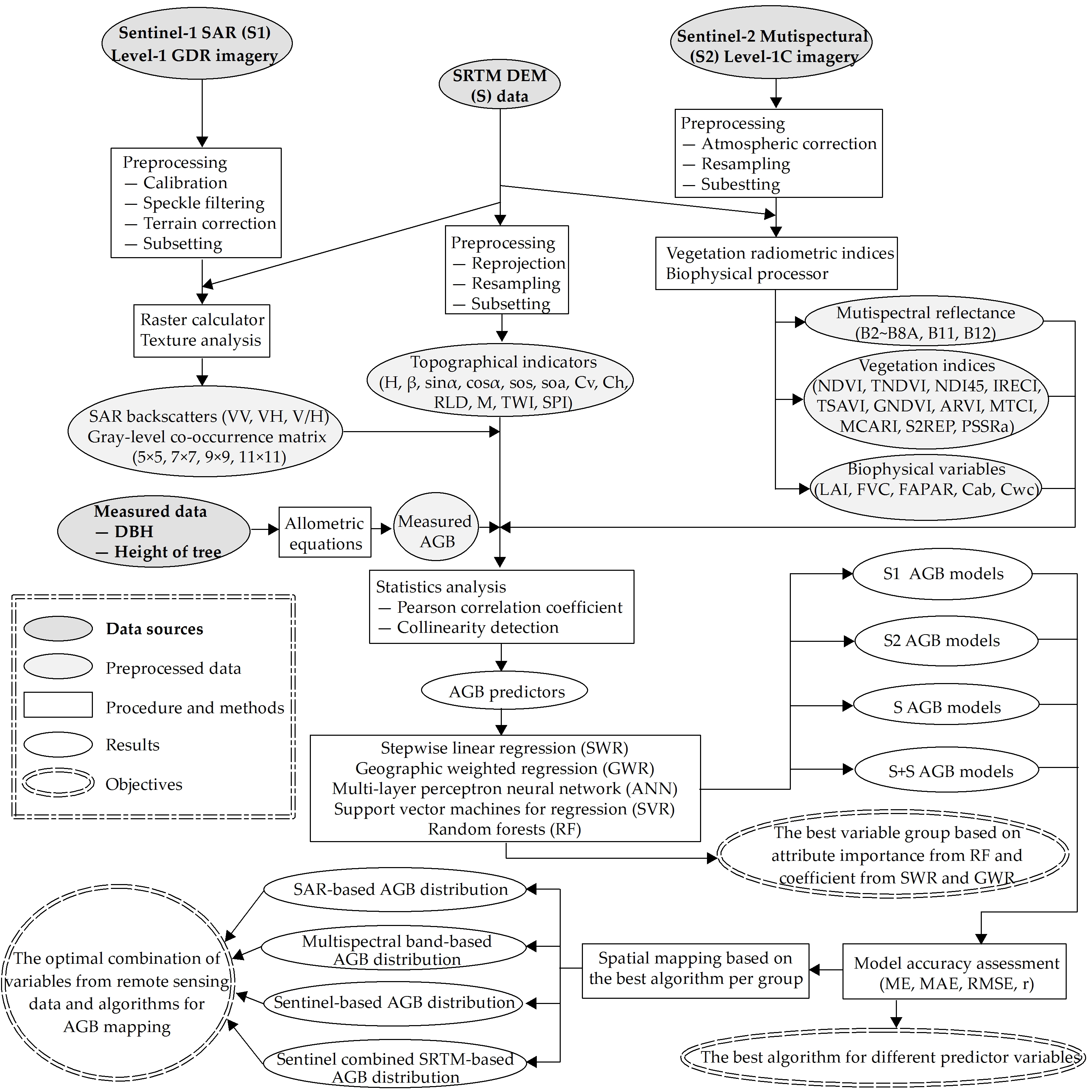
2. Materials and Methods

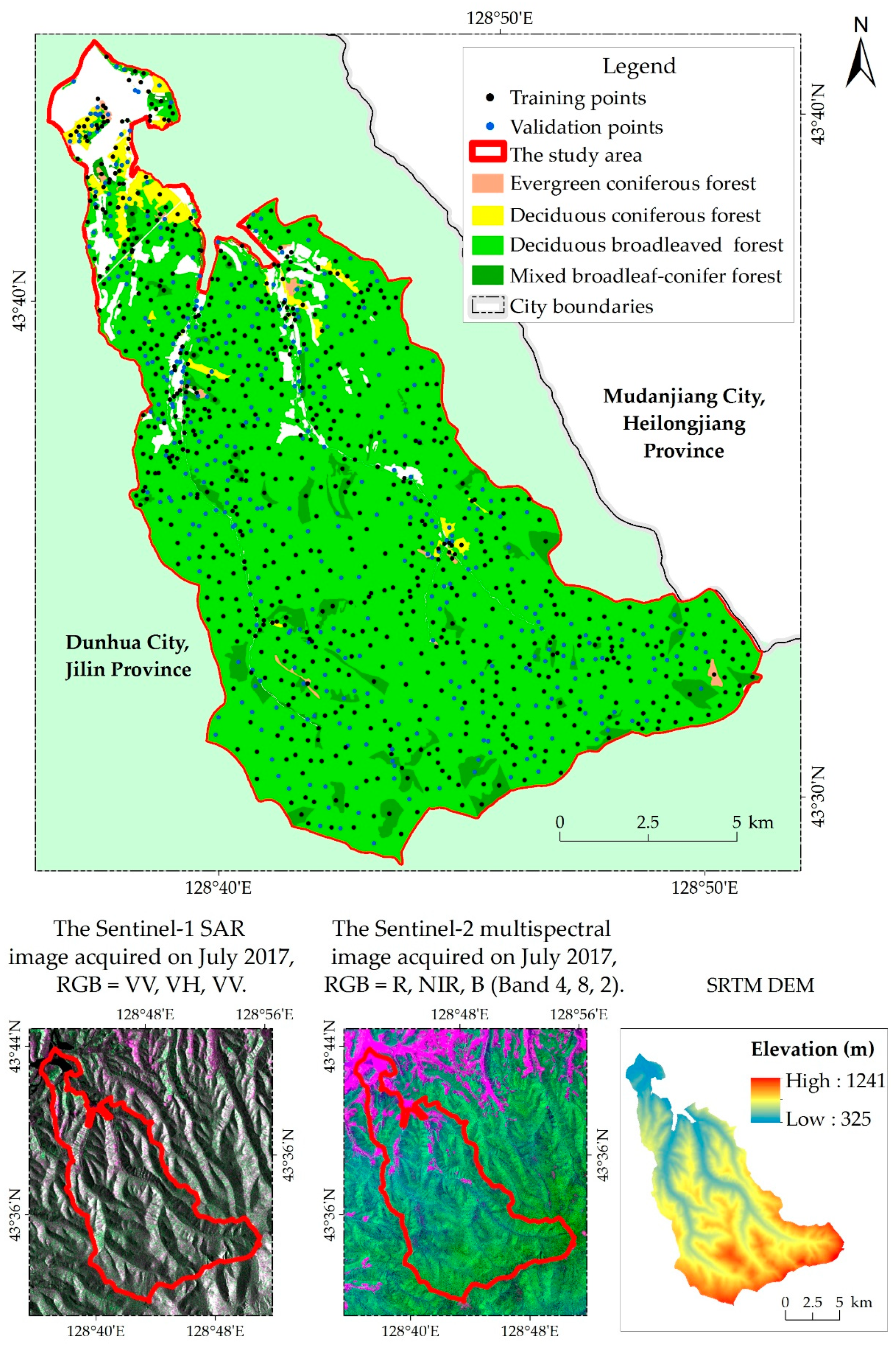
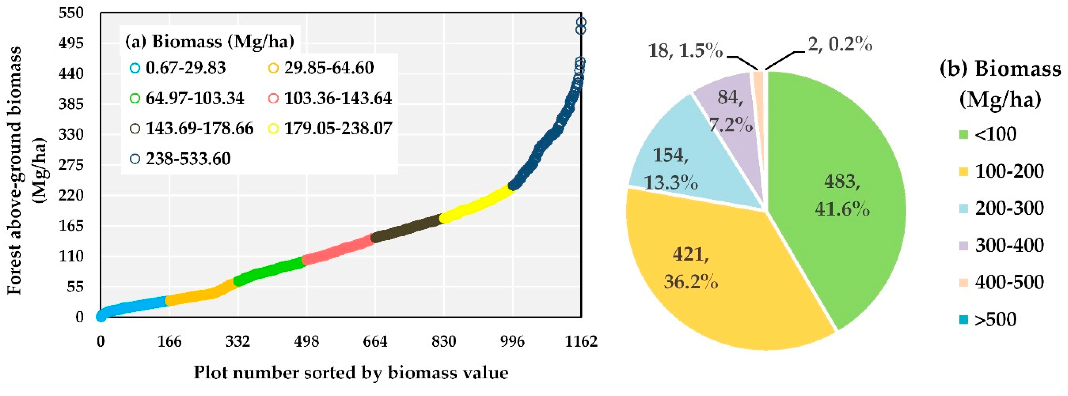
2.1. Study Site and Field-Measured Above-Ground Biomass

This study area covers 17,481 hectares of forests (Figure 1). The site is located within the eastern mountainous area of Jilin Province, northeast China. This region has a four-season, monsoon-influenced, humid continental climate, with an annual average temperature of 3.28 °C and an annual precipitation of 632 mm. Characterized by dense forest cover of the Changbai Mountains, the major forest types include deciduous broadleaved forest (90.7%) and mixed broadleaf-conifer forest (6.4%). Typical tree species include Mongolian oak (Quercus spp.), Betula platyphylla (Suk.), Tilia amurensis (Rupr.), and Fraxinus mandschurica (Rupr.).

The field campaign was carried out in July, 2017. The distribution of sampling plots was randomly generated, and non-forest areas were masked out. A total of 1,162 10 m × 10 m plots were located and sampled (Figure 1). The plots included 982 for broadleaved deciduous forests, 94 for mixed broadleaf-conifer forests, 59 for deciduous-coniferous forests, and 27 for evergreen coniferous forests. Based on allometric equations [45,46,47,48], measured diameter at breast height (1.3 m from the ground) and tree height, field-based forest AGB at each plot was calculated. The forest AGB samples were from 0.67 to 533.60 Mg·ha⁻¹, with the median value being between 103.36 to 143.64 Mg·ha⁻¹ (Figure 2a), and mainly below 200 Mg·ha⁻¹ with 77.8% (Figure 2b). The 1,162 sampling sites were randomly divided into training (n = 775) and validation (n = 387) sets (Figure 1) for establishing and examining the performance of the models.

2.2. Satellite Data Pre-Processing and Derived Variables

Sentinel series images were downloaded from the Copernicus Sentinel Scientific Data Hub (https://scihub.copernicus.eu/). The data included one Sentinel-1 C-band SAR VH and VV polarizations, and one Sentinel-2 MSI image. The SAR data were at a high-resolution (HR) Level-1 ground range detected (GRD) processing level with a pixel size of 10 m [37]. The Sentinel-2 Level 1C data were top-of-atmosphere reflectance, and they were processed for orthorectification and registration [38]. The MSI data had 13 spectral bands and were in 10 m (bands 2–4, 8), 20 m (band 5–7, 8a, 11–12), and 60 m (band 1, 9–10) spatial resolutions, respectively [38]. SRTM DEM data at a 30 m resolution were obtained from USGS were acquired (https://earthexplorer.usgs.gov/).

The procedures were illustrated in Figure 3. SNAP software (version 6.0, European Space Agency) was used to pre-process the Sentinel-1 and Sentinel-2 images. The steps based on the Sentinel-1 Toolbox of acquiring an accurate radar intensity backscatter coefficient with a map projection from the SAR images consisted of image calibration, speckle reduction using the Refined Lee Filter, and terrain correction by the Range-Doppler [36,49]. A bottom-of-atmosphere-corrected reflectance image was atmospherically corrected and processed from the Sentinel-2 Level 1C data by the radiative transfer model-based SEN2COR atmospheric correction processor (version 2.5.5, European Space Agency). The pre-processed Sentinel series images and the SRTM DEM data were registered into UTM Zone 52 WGS84 projection, and resampled to 10 m pixel sizes.

Uncertainties for the estimated AGB have been considered an important issue associated with modeling, based on remote sensing-derived variables [50,51]. For example, reported studies suggested that improved spatial resolution from the Sentinel series helped to reduce the uncertainty, and improved the accuracy of AGB mapping at finer scale [52,53]. Promising results demonstrated that texture measurement of SAR data with higher spatial resolution could improve biomass estimation [54,55]. However, uncertainties in implementing the texture measurement for biomass estimation were reported, due to the selection of window size [56,57]. Vegetation indices and biophysical variables are strongly related to reflectance, but they showed uncertainties for the estimated AGB in spectral sensitivity [58,59]. The reported study suggested that the red edge bands of Sentinel-2 (band 5, 6, 7, and 8A) were sensitive to phenological dynamics in vegetation, and that they were helpful for reducing the uncertainty [60,61]. In this study, 121 variables, including those that were suggested to be helpful in reducing uncertainties in forest AGB estimation, were selected and extracted for comparison evaluation [48,54,55,56,57,60,61,62,63,64]. A total of 109 variables were derived from the Sentinel series images, including 83 from Sentinel-1 SAR and 26 from Sentinel-2 MSI, and 12 topographic indices from SRTM DEM were also included (

Table 1. Remote sensing indices from the Sentinel series and SRTM digital elevation model (DEM) data for AGB mapping.

Source Image	Relevant Variables		Description
Sentinel-1 10 m resolution	Polarization	VV	Vertical transmit-vertical channel
		VH	Vertical transmit-horizontal channel
		V/H 1	VV/VH
	Texture 2	VV/VH_CON5/7/9/11	Contrast
		VV/VH_DIS5/7/9/11	Dissimilarity
		VV/VH_HOM5/7/9/11	Homogeneity
		VV/VH_ASM5/7/9/11	Angular second moment
		VV/VH_ENE5/7/9/11	Energy
		VV/VH_MAX5/7/9/11	Maximum probability
		VV/VH_ENT5/7/9/11	Entropy
		VV/VH_MEA5/7/9/11	Gray-level co-occurrence matrix (GLCM) mean
		VV/VH_VAR5/7/9/11	GLCM variance
		VV/VH_COR5/7/9/11	GLCM correlation
Sentinel-2 10 m resolution	Multispectral bands	B2	Blue, 490 nm
		B3	Green, 560 nm
		B4	Red, 665 nm
		B5	Red edge, 705 nm
		B6	Red edge, 749 nm
		B7	Red edge, 783 nm
		B8	Near infrared, 842 nm
		B8a	Near infrared, 865 nm
		B11	Short-wave infrared, 1610 nm
		B12	Short-wave infrared, 2190 nm
	Vegetation indices 3	NDVI	Normalized difference vegetation index, (B8 − B4)/(B8 + B4)
		NDI45	Normalized difference vegetation index with bands 4 and 5, (B5 − B4)/(B5 + B4)
		IRECI	Inverted red-edge chlorophyll index, (B7 − B4)/(B5/B6)
		TNDVI	Transformed normalized difference vegetation index, [(B8 − B4)/(B8 + B4) + 0.5]1/2
		TSAVI	Transformed soil adjusted vegetation index, 0.5 × (B8 − 0.5 × B4 − 0.5)/(0.5 × B8 + B4 − 0.15)
		GNDVI	Green normalized Difference vegetation index, (B7 − B3)/(B7 + B3)
		ARVI	Atmospherically resistant vegetation index, [B8 − (2 × B4 − B2)]/[B8 + (2 × B4 − B2)]
		MTCI	Medium-resolution imaging spectrometer terrestrial chlorophyll index, (B6 − B5)/(B5 − B4)
		MCARI	Modified chlorophyll absorption ratio index, [(B5 − B4) − 0.2 × (B5 − B3)] × (B5 − B4)
		S2REP	Sentinel-2 red-edge position index, 705 + 35 × [(B4 + B7)/2 − B5] × (B6 − B5)
		PSSRa	Pigment specific simple ratio chlorophyll index, B7/B4
	Vegetation biophysical variables 3	LAI	Leaf area index
		FVC	Fraction of vegetation cover
		FAPAR	Fraction of absorbed photosynthetically active radiation
		Cab	Chlorophyll content in the leaf
		Cwc	Canopy water content
SRTM DEM 30 m resolution	Elevation	H	Elevation
	First order micro topographic factors 4–8	β	Slope
		sinα	Sine of aspect, the extent of the location toward the east
		cosα	Cosine of aspect, the extent of the location toward the north
	Second order micro topographic factors 4–8	sos	Slope of slope, the curvature of the surface
		soa	Slope of aspect, the curvature of the contour line
		Cv	Profile curvature
		Ch	Plan curvature
	Hybrid macro topographic factors 4–8	RLD	Relief of land surface, Hmax−Hmin
		M	Surface roughness
		TWI	Topographic wetness index, Ln[Ac9/tanβ],
		SPI	Stream power index, Ln[Ac × tanβ × 100]

¹ Berninger et al. (2018); Bourgoin et al. (2018) [15,67]; ² Gray-level co-occurrence matrix (GLCM) of four size windows (i.e., 5 × 5, 7 × 7, 9 × 9, 11 × 11), Haralick et al. (1973) [68]; ³ SNAP (2016) [63]; ⁴ Jacob (1999) [69]; ⁵ Murdock and Dodds (2007) [70]; ⁶ Tang and Yang (2013) [62]; ⁷ Hou et al. (2014) [71]; ⁸ Xu (2015) [72]; ⁹ Ac is the catchment area directed to the vertical flow.

). The variables derived from the Sentinel series were conducted in the Sentinel-1 and Sentinel-2 Toolboxes of SNAP, and that from SRTM DEM were calculated in Spatial Analyst of ArcGIS (Figure 3). The biophysical variables were also calculated in SNAP from their biophysical processor by the reflectance of bands 3–8A, band 11, band 12 and geometric parameters, which used a neural network algorithm based on the PROSAIL radiative transfer model [65,66].

2.3. Modeling Algorithms and Evaluation

Firstly, a pairwise Pearson’s product-moment correlation analysis was operated to determine the relationship between field-based AGB and multisensor-derived indices, and collinearity among variables. Then the variance inflation factor (VIF) was calculated to delete the redundancy among variables (Figure 3). Variables that were highly correlated (r ≥ 0.8), and that had high VIF (VIF ≥ 10) in regression analysis were excluded from predictors of the modeling [48,73]. Those analyses were performed using SPSS (version 21.0, IBM, Armonk, NY, USA).

Sentinel series and SRTM DEM data were composed into four variable groups, including S1, S2, S, and S + S (Figure 3). The first group of variables (S1) was related to AGB with Sentinel-1 SAR polarization channels (i.e., VH and VV) and texture characteristics in four window sizes. The second group of variables (S2) was related AGB with Sentinel-2 multispectral bands, vegetation indices, and biophysical variables. The third group of variables was a combination of S1 and S2. The fourth group of variables used the factors of the combination of S1, S2, and topographic indices derived from SRTM DEM.

The five tested algorithms were listed in

Table 2. Linear regression and machine learning algorithms used in the study. The algorithms are available from SPSS, GWR, and WEKA software [76,77,78].

Algorithms	Software	Key Description	Necessary Parameters
Stepwise regression (SWR)	SPSS	Linear Regression in Analyze	Stepwise method
Geographically weighted regression (GWR)	GWR	Geographically Weighted Regression	Model type, Kernel type, Bandwidth selection method and Selection criteria
Artificial neural network (ANN)	WEKA	Multilayer Perceptron in Functions, Backpropagation to classify instances	Hidden layers, Learning rate, Momentum and Training time
Support vector machine for regression (SVR)		SMOreg in Functions, Support vector machine for regression	C (the regularization parameter), Kernel and its σ (the bandwidth parameter), Regoptimizer (the learning algorithm)
Random Forest (RF)		Random Forest in Trees, Construction a forest of random trees	Numfeatures (the number of randomly selected predictor variables at each node), Numiterations (the number of trees to grow in the forest)

. Linear regression algorithms included SWR and GWR, which were implemented in SPSS and GWR software (version 4.0, Ritsumeikan University, Kyoto, Japan), respectively. SWR is a global fitting regression model. SWR selects vital variables automatically. The contribution of variables to SWR can be determined by the coefficients [74]. GWR estimates individual parameters for each estimation location as a spatial model, the closer to the location of an observation, the greater the weight in a GWR model [75].

Machine learning algorithms were modeled in WEKA software (version 3.8, The University of Waikato, Hamilton, NZ). The ANN is a multi-layer perception neural network. Its architecture consists of input, hidden, and output layers, along with interconnection weights characterizing the connection strength. The algorithm takes the back-propagation learning rule to minimize the mean square error between the desired target and the actual output vectors [79]. The initial weights are assigned randomly, and when developing the network, the interconnection weights are adjusted to minimize the prediction error. SVR can construct an optimal hyperplane by projecting the data onto a new hyperspace based on means of kernel functions. The hyperplane can fit data with a modeling function that minimizes empirical risk and complexity when representing non-linear patterns [80].

RF combines bagging with random variable selections at each node to iteratively generate a large group of classification and regression trees. Every node in trees is a condition on a single feature, designed to split the dataset into two. Impurity is a measure that is based on the locally optimal condition that is chosen. For regression trees, it is variance. Thus, when training a tree, it can be computed to learn how much each feature decreases the weighted impurity in a tree. For a forest, the impurity decrease from each feature can be averaged, and the features are ranked according to this measure. In other words, the attribute importance in RF algorithms were calculated based on the mean decrease variance. The classification output represents an average from the whole ensemble for regression. Hence, it achieves a more robust result than a single classification tree that is produced by a single model run [81].The performances of SWR, GWR, ANN, SVR, and RF algorithms of each variables group were tested and compared, based on the root mean squared error (RMSE, Equation (1)), mean absolute error (MAE, Equation (2)), mean error (ME, Equation (3)), and correlation coefficient between the measured and predicted AGB (r, Equation (4)) [36,82]. The algorithm with the highest accuracy was selected for use in the predictive mapping of the AGB distribution in each group of variables. Four predictive maps were produced, which were derived from S1, S2, S, and S + S variables.

$$\mathrm{RMSE}=\sqrt{{\displaystyle {\sum }_1^n\frac{{(y_i\sum {\widehat{y}}_i)}^2}{n}}}$$

(1)

$$\mathrm{MAE}={\displaystyle \sum _1^n\frac{\left|y_i-{\widehat{y}}_i\right|}{n}}$$

(2)

$$\mathrm{ME}={\displaystyle \sum _1^n\frac{(y_i-{\widehat{y}}_i)}{n}}$$

(3)

$$r=\frac{{\displaystyle \sum _{i=1}^n(y_i-\overline{y})({\widehat{y}}_i-\overline{\widehat{y}})}}{\sqrt{{\displaystyle \sum _{i=1}^n(y_i-\overline{y})}}\sqrt{{\displaystyle \sum _{i=1}^n({\widehat{y}}_i-\overline{\widehat{y}})}}}$$

(4)

where ${\widehat{y}}_i$ is the estimated AGB value of each model, $y_i$ is the measured AGB value, and n is 387 in this study. The RMSE, MAE, and ME should be as small as possible, while r should be larger.

3. Results

3.1. Relationship between Field-Measured Biomass with Sentinel-Based and Topographical Variables

Among the S1 variables, 54 were significantly related to forest AGB (p < 0.05), including two backscatter values (VV, VH), four window sizes of VH_MEA, VH_VAR, VH_COR, and all 10 texture variables of VV. The backscatter values were positively related to AGB. With the growth of the window size, the r values of those 13 texture variables increased. Except for four sizes of VV_CON, VV_DIS and VV_ENT were negatively related to AGB, and the other 40 texture variables showed positive correlations. In other words, increasing the smoothness and the order of the VV backscatter indicated the decrease of the forest AGB. The top five AGB-related S1 variables were VV_ASM₁₁, VV_ENE₁₁, VV_MAX₁₁, VV_ENT₁₁, and VV_HOM₁₁.

As for S2, 21 variables were significantly related to forest AGB, excluding B5, 12, TSAVI, S2REP, and Cwc. The reflectance of B2–B4 were negatively related to AGB, while the other 18 variables showed the positive correlation. The reflectance of B2, NDI45, PSSRa, MCARI, and GNDVI displayed the strongest correlation with AGB. The vegetation indices that were calculated and synthesized by characteristic bands of S2 to monitor the chlorophyll of the vegetation were more distinguished and important for predicting forest AGB.

There were four topographical variables, i.e., H, M, TWI, and SPI, that obtained significant correlation with forest AGB, while impacts from the other eight factors were marginal. Elevation and wetness derived from SRTM DEM showed a positive influence on the increase of AGB; however, the surface roughness was negative. Hybrid macro-topographic indicators, as well as elevation, were more useful than other variables from SRTM DEM.

Above all, 79 variables acquired from Sl, S2, and SRTM DEM explained the valid information of forest AGB. Based on the average response of the entire samples, elevation, the texture characteristics of the VV channel in the 11×11-pixel window size, and the vegetation indices were comparatively vital for the forest AGB prediction.

3.2. Modeling Forest AGB

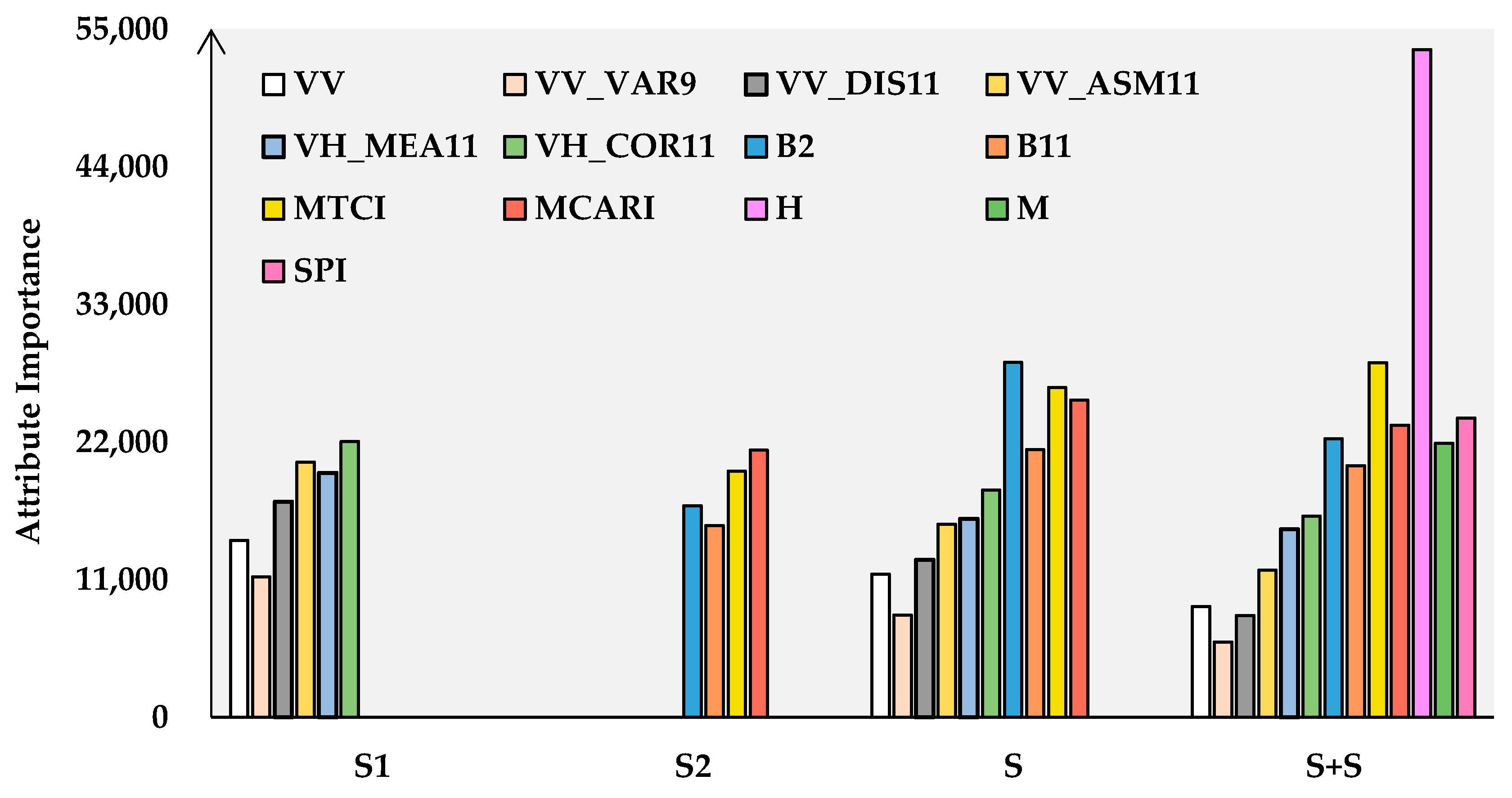
3.2.1. Predictors Selection and Descriptive Statistics

Based on the result from Section 3.1, 42 variables that had p values for the correlation analysis with AGB were above 0.05 were excluded. Then, 64 variables that had r values of the correlation analysis among predictors above 0.8 were disposed from the remaining 79 variables. Specifically, r values among VH_MEA and VH_VAR of four window sizes, as well as VH, were above 0.8, so that VH_MEA₁₁ with the highest r values of the correlation analysis with AGB was chosen as a predictor. Similarly, VH_COR₁₁ was chosen from VH_COR of four window sizes, then VV_DIS₁₁ was selected from VV_CON and VV_DIS of four window sizes, and VV_ASM₁₁ was selected from VV_HOM_5/7/9/11, VV_ASM_5/7/9/11, VV_ENE_5/7/9/11, VV_MAX_5/7/9/11 and VV_ENT_5/7/9/11, while VV_VAR₉ was elected from VV_MEA_5/7/9/11, VV_VAR_5/7/9/11 and VV_COR_5/7/9/11. B2 was selected rather than B3, B4, NDI45, and PSSRa, and B6 was chosen on behalf of B7, B8, B8A, IRECI, LAI, FVC, FAPAR, and Cab. The GDNVI was selected, on behalf of NDVI, TNDVI, and ARVI. As for the topographical variables, SPI was chosen rather than TWI. Among the remaining 15 variables, B6 and GNDVI, whose VIF exceeded the threshold of 10 were deleted. The predictors involved in modeling were the following 13 shown in

Table 3. Descriptive statistics of field-measured forest AGB, Sentinel-based, and topographical predictors.

	Mean	Median	SD 2	CV 3 (%)	Kurtosis	Skewness	Min	Max	r
AGBall 1	136.90	121.57	100.07	73	0.49	0.92	0.67	533.60	1
AGBt 1	132.51	117.85	97.92	74	0.86	0.99	2.88	533.60	/
AGBv 1	145.69	127.83	103.81	71	−0.07	0.77	0.67	433.24	/
VV	0.17	0.14	0.11	65	18.20	3.18	0.01	1.21	0.06 *
VV_VAR9	1894.57	1922.00	136.21	7	90.72	−8.58	9.21	1922.00	0.14 **
VV_DIS11	0.46	0.00	1.84	402	62.39	7.09	0.00	25.40	−0.15 **
VV_ASM11	3.52	4.00	1.04	30	3.26	−2.14	0.02	4.00	0.20 **
VH_MEA11	31.34	28.30	18.03	58	–1.24	0.25	0.00	62.00	0.11 **
VH_COR11	0.91	0.95	0.11	12	11.70	−2.80	0.00	1.00	0.19 **
B2	0.04	0.04	0.01	17	6.18	1.67	0.02	0.08	−0.20 **
B11	0.17	0.17	0.02	11	9.24	−0.70	0.03	0.26	0.08 *
MTCI	4.48	4.61	0.80	18	15.59	−1.43	–2.01	11.93	0.07 *
MCARI	0.11	0.11	0.02	22	2.13	−0.51	0.01	0.20	0.16 **
H	670.10	654.00	188.87	28	−0.70	0.39	339.00	1187.00	0.34 **
M	1.03	1.03	0.03	3	5.47	1.77	1.00	1.24	−0.07 *
SPI	3.79	4.18	2.77	73	−0.19	0.15	0.00	13.45	0.06 *

¹ AGB_all, AGB_t, and AGB_v are the whole, model training, and model validation biomass samples, respectively. ² SD means the standard deviation. ³ CV represents the coefficient of variation, which is defined as the ratio of the standard deviation to the mean. *denotes significance with a p-value of the t-test being below 0.05; ** denotes strong significance with a p-value below 0.01.

. Their r values, which represent the simple linear relationship with AGB, were relatively low. It was revealed that combing predictors from multiple sources and modeling algorithms were necessary.

Table 3 displays the basic statistics of the measured AGB and the multiple remote sensor predictors used as explanatory variables. The AGB of all the samples varied from 0.67 to 533.60 Mg·ha⁻¹, with a standard deviation and coefficient of variation (CV) of 100.07 and 0.73, respectively, which indicated moderate variability. For the explanatory variables, the CV of surface roughness was 0.03, which showed the least variability. The CV of VV_DIS₁₁, SPI, VV, and VH_MEA₁₁ were 4.02, 0.73, 0.65, and 0.58, indicating a stronger variability than the other predictors, respectively. The kurtosis of AGB was 0.49, and the skewness was 0.92, indicating that the AGB data had an approximately normal distribution.

3.2.2. Linear Regression

The four SWR models automated the selection of the best explanatory variables based on different predictors groups (

Table 4. Summary of AGB models by SWR.

Group	Formula	p-Value of F-Test	Adjusted R2
S1	AGB = 12.589 ** × VV_ASM11 + 85.359 * × VH_COR11 + 14.621	<0.01	0.042
S2	AGB = −3801.981 ** × B2 + 678.913 ** × B11 + 155.048 **	<0.01	0.053
S	AGB = 15.361 × VV_ASM11 ** − 3927.917 ** × B2 + 548.177 × B11 ** − 8.468 *×MTCI + 166.187 **	<0.01	0.078
S + S	AGB = 6.335 × VV_ASM11 + 82.607 * × VH_COR11 + 1582.612 * × B2 + 309.763 * × B11 + 0.215 **×H − 273.557 ** × M + 2.563 ** × SPI + 57.209	<0.01	0.158

* denotes significance with a p-value of t-test below 0.05; ** denotes strong significance with a p-value below 0.01.

). According to the formula and the p-values of the F-test, the four SWR models were strongly significant, while the factors influencing forest AGB varied. Specifically, VV_ASM₁₁ and VH_COR₁₁ were factors of forest AGB based on S1 predictors, and their impacts were significantly active, which was consistent with the above correlation analysis. B2 and B11 represented S2 indices for predicting AGB and explaining its variation significant influence. In accordance with adjusted R², AGB predicted by the SWR model based on S2 fit the measured AGB better that that based on S1. When combining S1 and S2, MTCI became much more important by replacing VH_COR₁₁, and the effect of B2 turned out to be unclear, due to the insignificance of its coefficient. In regard to the S+S variables, all four predictors from S1 and S2 models were retained. Among three predictors from SRTM DEM, only elevation showed a significant impact. Overall, VV_ASM₁₁, B2, B11, and H were relatively essential for AGB modeling, based on the SWR algorithm, and the SWR model based on predictors from S + S explained more of the information on forest AGB then the other three, on the basis of the highest adjusted R².

The GWR models were the Gaussian approach, where the weight function was an adaptive Gaussian kernel. The models found the optimal bandwidth by using a golden section search and the corrected Akaike information criterion (AICc, small sample bias corrected AIC). The GWR was a local regression method whose parameters in the formula varied across the study area. The top three predictors with the largest absolute mean values of coefficients in each GWR model were recorded in

Table 5. Summary of AGB models by GWR.

Group	Top Three Ranked Predictors of Absolute Mean Values of Coefficients	Bandwidth	Adjusted R2	AICc
S1	VH_COR11, VV, VV_ASM11	88.72	0.302	13618.33
S2	B11, B2, MCARI	50.82	0.336	13566.47
S	B11, B2, MCARI	88.83	0.341	13572.94
S+S	B2, B11, M	80.29	0.351	13578.47

. B2 and B11 were relatively important in GWR modeling for predicting forest AGB in the study area. According to the values of the adjusted R² of four models, predictors from S2 were more influential than that from S1 on forest AGB prediction. However, the effective information decreased when S1 variables or topographic indices were added, as indicated by the lowest value of AICc of the S2 model, among the four.

To sum up, both global and local linear regression algorithms indicated that predictors from S2 performed better than those from S1. Combining all of the factors from S1, S2, and SRTM DEM improved the ability of the linear regression models to predict forest AGB.

3.2.3. Machine Learning Algorithms

The necessary parameters of machine learning models are shown in

Table 6. Summary of AGB models by ANN, SVR and RF.

	ANN				SVR		RF
Group	Learning Rate	Momentum	Training Time	Hidden Layers	C	σ	Features	Tree
S1	0.1	0.2	500	6	5	5	4	1000
S2	0.2	0.01	500	4	5	5	2	1000
S	0.1	0.1	500	7	5	5	5	1000
S+S	0.3	0.2	500	8	5	5	8	1000

. The optimized ANN architecture of the S1 model used 13 input nodes in the input layer, six nodes in the hidden layer with the unipolar sigmoid as the transfer function, and one node in the output layer (i.e., 13-16-1). Using the Levenberg–Marquardt learning algorithm, the best learning rate, momentum, and training time obtained were determined to be 0.1, 0.2, and 500, respectively. Likewise, the other three ANN models were built with parameters in Table 6. As for the SVR models, using the SMO (sequential minimal optimization) algorithm with Shevade et al. [83] and the RBF (radial basis function) kernel, the best parameters for C and σ that were obtained were both five and five, respectively. With a tree number of 1000, and feature numbers of four, two, five, and eight, the RF models based on S1, S2, S, and S+S were acquired, respectively.

The attribute importance for the four RF models was calculated based on the mean decrease variance, and illustrated in Figure 4. In detail, VH_COR₁₁ was the most important factor of the RF model based on the S1 predictors, which was in accordance with the linear regression models. In the S2 RF model, MCARI was the most needed predictor, which was different to the linear models. When integrating S1 and S2 to build the RF models, the attribute importance ranking of the S1 variables changed a little, which was that VH_MEA₁₁ turned out to be more important than VV_ASM₁₁. While the attribute importance ranking of the S2 variables changed, B2 surpassed MTCI and MCARI, and became the primary predictor. Additionally, predictors from S2 were more crucial than those from S1, due to the higher importance in the S model. After adding topographic indices to the S RF model, the attribute importance ranking of factors from S1 remained the same, while that from S2 changed, where MTCI was shown to be the most important among the S2 predictors. Elevation was the most essential factor, followed by MTCI and SPI. In short, predictors from S2 were more vital than that from S1, which was also found by linear models, and elevation from SRTM DEM contributed to a lot of RF modeling for predicting forest AGB.

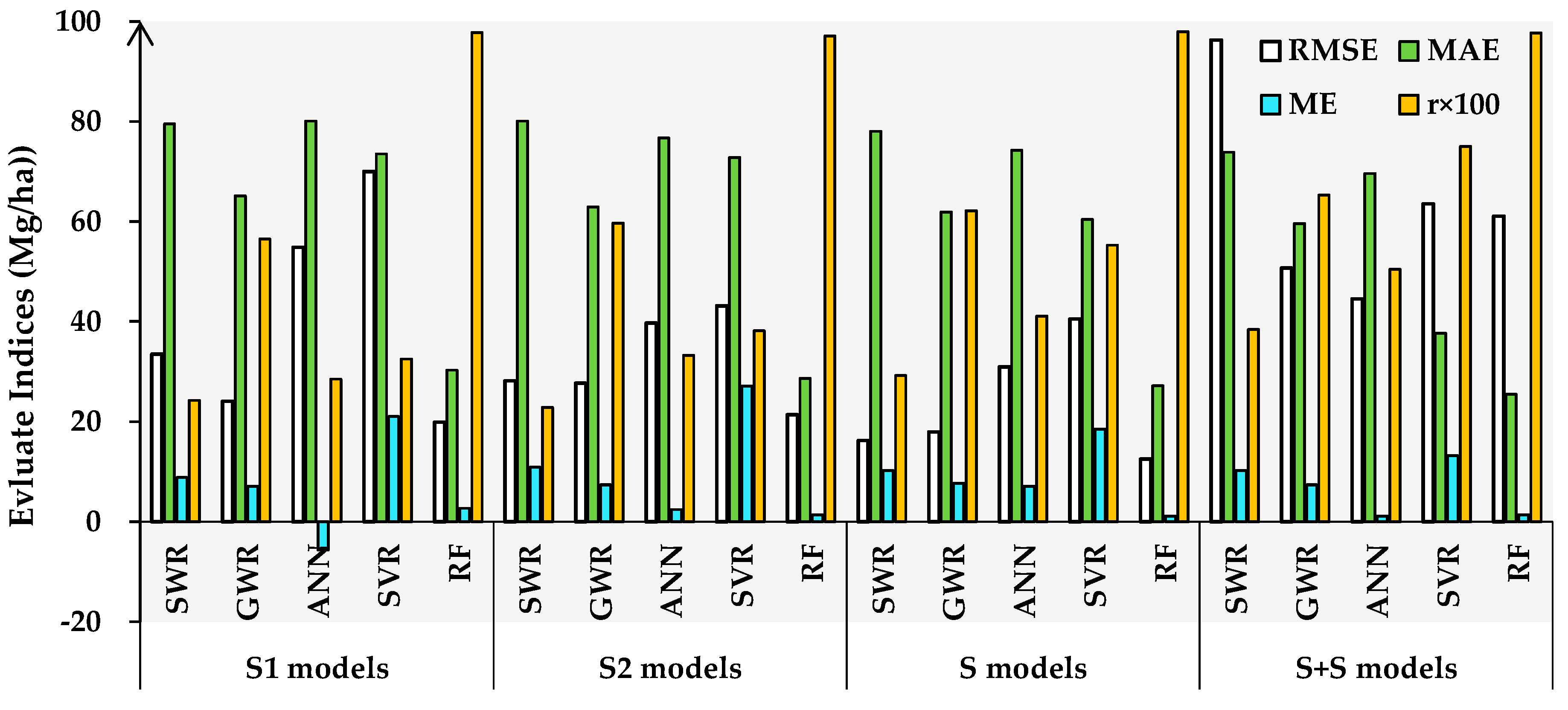
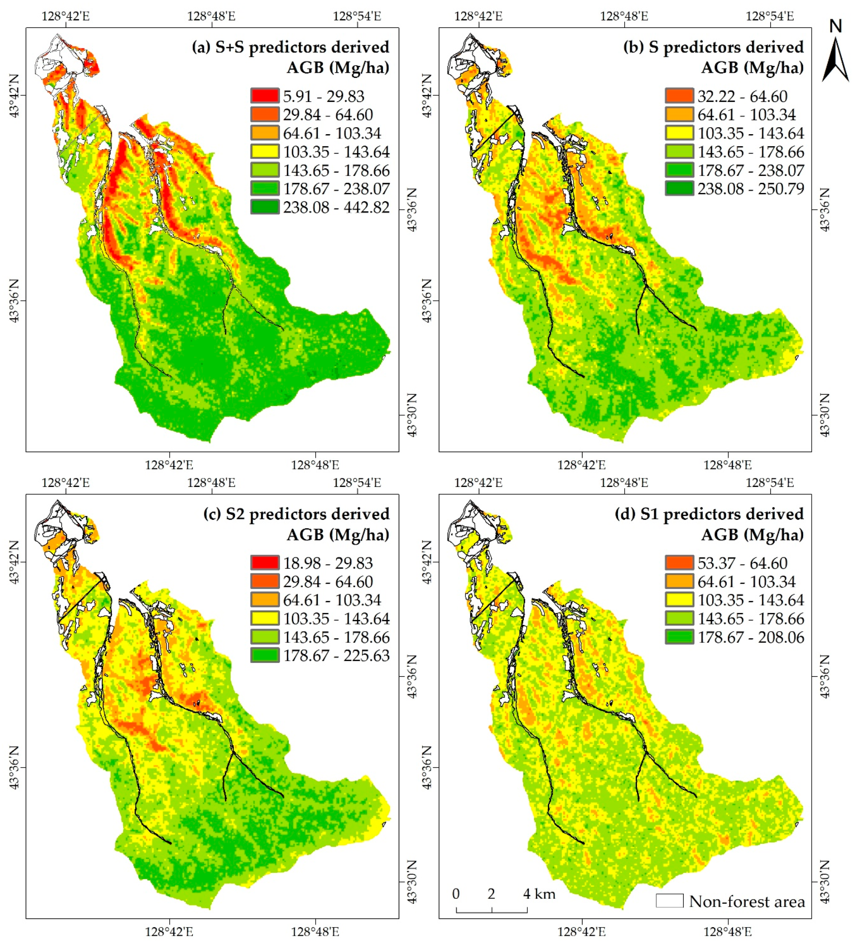
3.3. Models Assessment and Biomass Mapping.

Calculated by an independent validation dataset, the accuracies of the five algorithms were depicted in Figure 5. All five S1 models underestimated AGB, except for the ANN model. The S1 RF model, with the lowest RMSE (19.90 Mg·ha⁻¹), MAE (30.31 Mg·ha⁻¹), and ME (2.65 Mg·ha⁻¹) as well as the highest r (0.9781), was an algorithm chosen to predict forest AGB based on S1 indices. The S2 models all underestimated the AGB. The RF algorithm also was considered the optimal one, where the RMSE, MAE, ME, and r were 21.37, 28.61, 1.37 Mg·ha⁻¹, and 0.9715, respectively. Coupling the S1 and S2 explanatory variables, the accuracies of all the models increased, and the RF was also the most accurate algorithm with the lowest RMSE (12.51 Mg·ha⁻¹), MAE (27.15 Mg·ha⁻¹), and ME (1.15 Mg·ha⁻¹), as well as the highest r (0.9790). The models combining the explanatory variables from S1, S2, and SRTM DEM all showed the tendency for underestimation. Although the ANN algorithm obtained the lowest RMSE and ME among the S + S models, its value of ME was relatively high, and r was low. Thus, the RF model was selected again with the lowest MAE (25.48 Mg·ha⁻¹) and the highest r (0.9769), where the RMSE and ME were 61.11 and 1.39 Mg·ha⁻¹, respectively. In summary, all of the models underestimated forest AGB except for the ANN one based on the S1 factors, and four RF algorithms were selected to map forest AGB distribution.

The predicted values of forest AGB of the study area ranged from 5.91 to 442.82 Mg·ha⁻¹ (Figure 6). For a better comparison among the four models, the values were divided into seven levels by intervals of measured AGB values in Figure 2a. All maps showed that the southern part of the study area was a high AGB region, with values ranging from 208.06 to 442.82 Mg·ha⁻¹. Low AGB (5.91 to 53.37 Mg·ha⁻¹) zones were located close to non-forest areas. Comparing the predicted and measured AGB (Figure 2), the RF model built by multisource explanatory variables from S1, S2, and SRTM DEM performed the best (Figure 6a). The map produced from the RF model based on six S1 predictors displayed the fragmentation of AGB, where spatial distribution was rather random (Figure 6d). Although there were only four predictors from S2, they demonstrated better performance compared to S1 factors on forest AGB mapping by the RF algorithm (Figure 6c), but it was still difficult to predict high values of forest AGB (238–533.06 Mg·ha⁻¹, shown in Figure 2a). The distribution of forest AGB predicted by the RF model using S1 and S2 predictors (Figure 6b) was similar with that by the S2 RF model. This S model made progress in high values of forest AGB; however, it overestimated low values of AGB (0.67–29.83 Mg·ha⁻¹, shown in Figure 2a). It had a great improvement on the accuracy of forest AGB mapping, where topographic indices from SRTM DEM were joined to the explanatory variables of the RF model (Figure 6a). In detail, the distribution of the predicted values of forest AGB by the Sentinel series, combined with the SRTM DEM model depicted in Figure 6a, was relatively in keeping with the field data (Figure 2).

4. Discussion

4.1. Sentinel-Based and Topographical Predictors of Forest AGB Mapping

This study revealed that the relationships of the measured AGB with Sentinel-based and topographical predictors varied by modeling the algorithms according to parameters from the SWR and GWR formulas, and the attribute importance from RF models. VV_ASM₁₁ and VH_COR₁₁ were the most important variables among the S1 variables for explaining the observed spatial patterns of forest AGB both in the linear global and local regression, and this was also shown in the RF models. Texture features were usually calculated for forest AGB mapping, with one fixed window size [15,67,84]. It was helpful to note that the texture characteristics of the Sentinel SAR backscatters with a larger window size (i.e., 11 × 11) achieved a greater potential for mapping forest AGB, based on the correlation analysis. The backscatter coefficients of S1 and their calculation were useful as common predictors [36,85,86]. The study indicated that direct use of the backscatter coefficients from the SAR C band might not be appropriate. The lack of penetrability could affect biomass information retrieval. Meanwhile, the variation and disorder of backscatters showed in texture might be caused by vegetation diversity and density. These texture characteristics denoted a significant relationship with AGB. In other words, vegetation diversity and density was reflected as variation of backscatter texture, resulting in higher forest AGB. Some of the S2 variables showed a significant relationship with forest AGB [87,88,89]. This indicated that the selection of predictors were necessary for S2-based prediction. Owing to the acquisition from the band calculation, two vegetation indices were deleted in the S2 SWR model, while they showed a greater impact on GWR and RF modeling of forest AGB. It revealed that variables obtained from the operation of S2 multispectral bands, especially vegetation indices representing chlorophyll characteristics, were more efficient for complex regression algorithms, whereas the reflectance of multispectral bands as the direct information of S2 were more important for simple global linear modeling. However, collinearity and redundancy of the predictors decreased the effective information of models, and this pre-processing for modeling needs to be improved in future work. It was supposed that predictors were obtained by synthesizing indices such as principal component analysis, rather than simply deleting variables with lower correlation with forest AGB.

The strongest related predictor was elevation, as shown in Table 3 and Figure 4. The vital role of topography was also reported in other studies by influencing water and sunlight supply and storage [36,44,64]. As a proxy for the potential soil–water storage for vegetation [90], TWI was reported as being an important factor for estimating forest AGB, using nonlinear regression models [64]. However in this study, it was replaced by SPI, which was more relative to measured AGB. SPI was the third important predictor of the RF model (Figure 4), after H and MTCI, and it is also listed in the SWR model. It demonstrated that SPI was an essential predictor for forest AGB mapping. Due to the close correlation between AGB and TWI and SPI, it was proposed that both indices should be tested in other geographical settings that are different than this study. Surface roughness (M) was also a vital predictor in this study, both in linear regression and machine learning models, which had a greater influence than S1 predictors. Predictors from S2 were comparatively primary for forest AGB prediction. Factors from SRTM DEM were effective compared to that from S1 in complex AGB modeling, while S1 texture features were useful in simple AGB models. It is suggested that texture characteristics measured in an 11×11-pixel window of S1, and the reflectance and vegetation indices of S2, as well as elevation, SPI, TWI, and M be recommended predictors for forest AGB mapping.

4.2. Optimal Combination of Predictors and Modeling Algorithms

Based on the predictor selection in Section 3.2.1, the best predictors for forest AGB mapping were determined to be those listed in Table 3, which belong to the four variable groups, S1, S2, S and S + S. In contrast, the optimal modeling algorithm for predictors from the four variable groups were all the RF algorithm. This study revealed the powerful capacity of the RF algorithm to predict forest AGB, as in other reported studies [88,91,92,93]. The SVR algorithm, however, performed the worst for S1 variables, while the SWR algorithm performed the worst for S2 and S, as well as S+S modeling. Different from other studies [29,33,91], the performances of linear regression algorithms in this research were closer to that by machine learning. The improvement might be from the contribution of the localized spatial scale of the study, and the density of representative field samples of forest AGB. It was demonstrated that SVR algorithm was suitable for limited samples prediction, in agreement with other studies [25,48,94]. Figure 5 indicated that predictor variables were more important than algorithms for remote sensing-based estimations of forest AGB. The linear regression depended more on predictors than on machine learning algorithms.

L- and P-band SAR, as well as LiDAR were crucial for prediction of high forest AGB values. Although C band SAR and optical multispectral have demonstrated the saturation for detecting the sensibility of forest AGB, the Sentinel series, and SRTM DEM in fine-resolution with full coverage provided critical information for applications in comparison to forest AGB estimation.

5. Conclusions

Predictors from Sentinel-1 C band SAR, Sentinel-2 MSI, and SRTM DEM were extracted with a resolution of 10 m and divided into four variable groups. Five modeling algorithms, including SWR (a global linear regression), GWR (a local linear model), ANN, SVR, and RF, were built using 775 field measurements, and tested by 387 independent field samples. The results demonstrated that the RF algorithm was the best for predicting and mapping spatial patterns of AGB, with all groups of predictors in the study site. It also proposed that for texture characteristics in an 11 × 11-pixel window of Sentinel-1 SAR, the reflectance and vegetation indices of Sentinel-2 MSI, as well as elevation, SPI, TWI, and M from SRTM DEM were the vital predictors for explaining the observed variability of AGB. Sentinel-2 MSI were considered primary, and SRTM DEM were more important than Sentinel-1 SAR in complex AGB modeling, while texture features of SAR were useful in simple models. Predictor variables were more important than algorithms for improving the accuracy of AGB estimates. Machine learning models were less dependent on predictors than linear regression. Overall, the comparison assessment of this study provided a reference for the selection of combinations of predictors and algorithms for forest AGB modeling.

References

1. Pan, Y.; Birdsey, R.A.; Fang, J.; Houghton, R.; Kauppi, P.E.; Kurz, W.A.; Phillips, O.L.; Shvidenko, A.; Lewis, S.L.; Canadell, J.G.; et al. A large and persistent carbon sink in the world’s forests. Science 2011, 333, 988–993. [Google Scholar] [CrossRef] [PubMed]
2. Bloom, A.A.; Exbrayat, J.F.; van der Velde, I.R.; Feng, L.; Williams, M. The decadal state of the terrestrial carbon cycle: Global retrievals of terrestrial carbon allocation, pools, and residence times. Proc. Natl. Acad. Sci. USA 2016, 113, 1285–1290. [Google Scholar] [CrossRef] [PubMed]
3. Santi, E.; Paloscia, S.; Pettinato, S.; Fontanelli, G.; Mura, M.; Zolli, C.; Maselli, F.; Chiesi, M.; Bottai, L.; Chirici, G. The potential of multifrequency SAR images for estimating forest biomass in Mediterranean areas. Remote Sens. Environ. 2017, 200, 63–73. [Google Scholar] [CrossRef]
4. Fotis, A.T.; Murphy, S.J.; Ricart, R.D.; Krishnadas, M.; Whitacre, J.; Wenzel, J.W.; Queenborough, S.A.; Comita, L.S. Above-ground biomass is driven by mass-ratio effects and stand structural attributes in a temperate deciduous forest. J. Ecol. 2018, 106, 561–570. [Google Scholar] [CrossRef]
5. Erb, K.H.; Kastner, T.; Plutzar, C.; Bais, A.L.S.; Carvalhais, N.; Fetzel, T.; Gingrich, S.; Haberl, H.; Lauk, C.; Niedertscheider, M.; et al. Unexpectedly large impact of forest management and grazing on global vegetation biomass. Nature 2018, 553, 73–76. [Google Scholar] [CrossRef]
6. Sedjo, R. The carbon cycle and global forest ecosystem. Water Air Soil Poll. 1993, 70, 295–307. [Google Scholar] [CrossRef]
7. Motlagh, M.G.; Kafaky, S.B.; Mataji, A.; Akhavan, R. Estimating and mapping forest biomass using regression models and Spot-6 images (case study: Hyrcanian forests of north of Iran). Environ. Monit. Assess. 2018, 190, 352–365. [Google Scholar] [CrossRef]
8. Brown, S.; Schroeder, P.; Birdsey, R. Aboveground biomass distribution of US eastern hardwood forests and the use of large trees as an indicator of forest development. For. Ecol. Manag. 1997, 96, 37–47. [Google Scholar] [CrossRef]
9. Zhao, P.; Lu, D.; Wang, G.; Wu, C.; Huang, Y.; Yu, S. Examining spectral reflectance saturation in landsat imagery and corresponding solutions to improve forest aboveground biomass estimation. Remote Sens. 2016, 8, 469. [Google Scholar] [CrossRef]
10. Gonzalez, P.; Asner, G.P.; Battles, J.J.; Lefsky, M.A.; Waring, K.M.; Palace, M. Forest carbon densities and uncertainties from Lidar, QuickBird, and field measurements in California. Remote Sens. Environ. 2010, 114, 1561–1575. [Google Scholar] [CrossRef]
11. Minha, D.H.T.; Ndikumana, E.; Vieilledent, G.; McKey, D.; Baghdadi, N. Potential value of combining ALOS PALSAR and Landsat-derived tree cover data for forest biomass retrieval in Madagascar. Remote Sens. Environ. 2018, 213, 206–214. [Google Scholar] [CrossRef]
12. Sadeghi, Y.; St-Onge, B.; Leblon, B.; Prieur, J.F.; Simard, M. Mapping boreal forest biomass from a SRTM and TanDEM-X based on canopy height model and Landsat spectral indices. Int. J. Appl. Earth. Obs. Geoinf. 2018, 68, 202–213. [Google Scholar] [CrossRef]
13. Saatchi, S.S.; Harris, N.L.; Brown, S.; Lefsky, M.; Mitchard, E.T.A.; Salas, W.; Zutta, B.R.; Buermann, W.; Lewis, S.L.; Hagen, S.; et al. Benchmark map of forest carbon stocks in tropical regions across three continents. Proc. Natl. Acad. Sci. USA 2011, 108, 9899–9904. [Google Scholar] [CrossRef] [Green Version]
14. Thurner, M.; Thurner, M.; Beer, C.; Santoro, M.; Nuno, C.; Wutzler, T.; Schepaschenko, D.; Shvidenko, A.; Kompter, E.; Ahrens, B.; et al. Carbon stock and density of northern boreal and temperate forests. Glob. Ecol. Biogeogr. 2014, 23, 297–310. [Google Scholar] [CrossRef]
15. Berninger, A.; Lohberger, S.; Stängel, M.; Siegert, F. SAR-based estimation of above-ground biomass and its changes in tropical forests of Kalimantan using L- and C-band. Remote Sens. 2018, 10, 831. [Google Scholar] [CrossRef]
16. Ene, L.T.; Naesset, E.; Gobakken, T.; Gregoire, T.G.; Stahl, G.; Holm, S. A simulation approach for accuracy assessment of two-phase post-stratified estimation in large-area LiDAR biomass surveys. Remote Sens. Environ. 2013, 133, 210–224. [Google Scholar] [CrossRef]
17. Searle, E.B.; Chen, H.Y.H. Tree size thresholds produce biased estimates of forest biomass dynamics. For. Ecol. Manag. 2017, 400, 468–474. [Google Scholar] [CrossRef]
18. Avitabile, V.; Baccini, A.; Friedl, M.A.; Schmullius, C. Capabilities and limitations of Landsat and land cover data for aboveground woody biomass estimation of Uganda. Remote Sens. Environ. 2012, 117, 366–380. [Google Scholar] [CrossRef]
19. Baccini, A.; Goetz, S.J.; Walker, W.S.; Laporte, N.T.; Sun, M.; Sulla-Menashe, D.; Hackler, J.; Beck, P.S.A.; Dubayah, R.; Friedl, M.A.; et al. Estimated carbon dioxide emissions from tropical deforestation improved by carbon-density maps. Nat. Clim. Chang. 2012, 2, 182–185. [Google Scholar] [CrossRef]
20. Joshi, N.; Mitchard, E.T.A.; Schumacher, J.; Johannsen, V.K.; Saatchi, S.; Fensholt, R. L-band SAR backscatter related to forest cover, height and aboveground biomass at multiple spatial scales across Denmark. Remote Sens. 2015, 7, 4442–4472. [Google Scholar] [CrossRef]
21. Muukkonen, P.; Heiskanen, J. Biomass estimation over a large area based on standwise forest inventory data and ASTER and MODIS satellite data: A possibility to verify carbon inventories. Remote Sens. Environ. 2007, 107, 617–624. [Google Scholar] [CrossRef]
22. Zhao, P.P.; Lu, D.S.; Wang, G.X.; Liu, L.J.; Li, D.Q.; Zhu, J.R.; Yu, S.Q. Forest aboveground biomass estimation in Zhejiang Province using the integration of Landsat TM and ALOS PALSAR data. Int. J. Appl. Earth Obs. 2016, 53, 1–15. [Google Scholar] [CrossRef]
23. Shao, Z.F.; Zhang, L.J.; Wang, L. Stacked sparse autoencoder modeling using the synergy of airborne LiDAR and satellite optical and SAR data to map forest above-ground biomass. IEEE J.-STARS 2017, 10, 5569–5582. [Google Scholar] [CrossRef]
24. Huang, H.B.; Liu, C.X.; Wang, X.Y.; Zhou, X.L.; Gong, P. Integration of multi-resource remotely sensed data and allometric models for forest aboveground biomass estimation in China. Remote Sens. Environ. 2019, 221, 225–234. [Google Scholar] [CrossRef]
25. Fassnacht, F.E.; Hartig, F.; Latifi, H.; Berger, C.; Hernandez, J.; Corvalan, P.; Koch, B. Importance of sample size, data type and prediction method for remote sensing-based estimations of aboveground forest biomass. Remote Sens. Environ. 2014, 154, 102–114. [Google Scholar] [CrossRef]
26. Rivera, J.; Verrelst, J.; Delegido, J.; Veroustraete, F.; Moreno, J. On the semi-automatic retrieval of biophysical parameters based on spectral index optimization. Remote Sens. 2014, 6, 4927–4951. [Google Scholar] [CrossRef]
27. Peddle, D.R.; Hall, F.G.; LeDrew, E.F. Spectral mixture analysis and geometric-optical reflectance modeling of boreal forest biophysical structure. Remote Sens. Environ. 1999, 67, 288–297. [Google Scholar] [CrossRef]
28. Atzberger, C. Object-based retrieval of biophysical canopy variables using artificial neural nets and radiative transfer models. Remote Sens. Environ. 2004, 93, 53–67. [Google Scholar] [CrossRef]
29. Yue, J.B.; Feng, H.K.; Yang, G.J.; Li, Z.H. A comparison of regression techniques for estimation of above-ground winter wheat biomass using near-surface spectroscopy. Remote Sens. 2018, 10, 66. [Google Scholar] [CrossRef]
30. Zheng, D.L.; Rademacher, J.; Chen, J.Q.; Crow, T.; Bresee, M.; Moine, J.L.; Ryu, S.R. Estimating aboveground biomass using Landsat 7 ETM+ data across a managed landscape in northern Wisconsin, USA. Remote Sens. Environ. 2004, 93, 402–411. [Google Scholar] [CrossRef]
31. Propastin, P. Modifying geographically weighted regression for estimating aboveground biomass in tropical rainforests by multispectral remote sensing data. Int. J. Appl. Earth Obs. 2012, 18, 82–90. [Google Scholar] [CrossRef]
32. Laurin, G.V.; Chen, Q.; Lindsell, J.A.; Coomes, D.A.; Frate, F.D.; Guerriero, L.; Pirotti, F.; Valentini, R. Above ground biomass estimation in an African tropical forest with lidar and hyperspectral data. ISPRS J. Photogramm. Remote Sens. 2014, 89, 49–58. [Google Scholar] [CrossRef]
33. Gao, Y.K.; Lu, D.S.; Li, G.Y.; Wang, G.X.; Chen, Q.; Liu, L.J.; Li, D.Q. Comparative analysis of modeling algorithms for forest aboveground biomass estimation in a subtropical region. Remote Sens. 2018, 10, 627. [Google Scholar] [CrossRef]
34. Malenovsky, Z.; Rott, H.; Cihlar, J.; Schaepman, M.E.; Garcia-Santos, G.; Fernandes, R.; Berger, M. Sentinels for science: Potential of Sentinel-1, -2, and -3 missions for scientific observations of ocean, cryosphere, and land. Remote Sens. Environ. 2012, 120, 91–101. [Google Scholar] [CrossRef]
35. Torres, R.; Snoeij, P.; Geudtner, D.; Bibby, D.; Davidson, M.; Attema, E.; Potin, P.; Rommen, B.; Floury, N.; Brown, M.; et al. GMES Sentinel-1 mission. Remote Sens. Environ. 2012, 120, 9–24. [Google Scholar] [CrossRef]
36. Castillo, J.A.A.; Apan, A.A.; Maraseni, T.N.; Salmo, S.G. Estimation and mapping of above-ground biomass of mangrove forests and their replacement land uses in the Philippines using Sentinel imagery. ISPRS J. Photogramm. Remote Sens. 2017, 134, 70–85. [Google Scholar] [CrossRef]
37. Sentinel-1_Team. Sentinel-1 User Handbook; European Space Agency: Paris, France, 2013. [Google Scholar]
38. Sentinel-2_Team. Sentinel-2 User Handbook; European Space Agency: Paris, France, 2015. [Google Scholar]
39. Sibanda, M.; Mutanga, O.; Rouget, M. Examining the potential of Sentinel-2 MSI spectral resolution in quantifying above ground biomass across different fertilizer treatments. ISPRS J. Photogramm. Remote Sens. 2015, 110, 55–65. [Google Scholar] [CrossRef]
40. Laurin, G.V.; Puletti, N.; Hawthorne, W.; Liesenberg, V.; Corona, P.; Papale, D.; Chen, Q.; Valentini, R. Discrimination of tropical forest types, dominant species, and mapping of functional guilds by hyperspectral and simulated multispectral Sentinel-2 data. Remote Sens. Environ. 2016, 176, 163–176. [Google Scholar] [CrossRef] [Green Version]
41. Mura, M.; Bottalico, F.; Giannetti, F.; Bertani, R.; Giannini, R.; Mancini, M.; Orlandini, S.; Travaglini, D.; Chirici, G. Exploiting the capabilities of the Sentinel-2 multi spectral instrument for predicting growing stock volume in forest ecosystems. Int. J. Appl. Earth Obs. 2018, 66, 126–134. [Google Scholar] [CrossRef]
42. Rodríguez, E.; Morris, C.S.; Belz, J.E. A global assessment of the SRTM performance. Photogramm. Eng. Remote Sens. 2006, 72, 249–260. [Google Scholar] [CrossRef]
43. Simard, M.; Zhang, K.Q.; Rivera-Monroy, V.H.; Ross, M.S.; Ruiz, P.L.; Castaneda-Moya, E.; Twilley, R.R.; Rodriguez, E. Mapping height and biomass of mangrove forests in Everglades National Park with SRTM elevation data. Photogramm. Eng. Remote Sens. 2006, 72, 299–311. [Google Scholar] [CrossRef]
44. Su, Y.J.; Guo, Q.H.; Xue, B.L.; Hu, T.Y.; Alvarez, O.; Tao, S.L.; Fang, J.Y. Spatial distribution of forest aboveground biomass in China: Estimation through combination of spaceborne lidar, optical imagery, and forest inventory data. Remote Sens. Environ. 2016, 173, 187–199. [Google Scholar] [CrossRef] [Green Version]
45. Wang, C.K. Biomass allometric equations for 10 co–occurring tree species in Chinese temperate forests. Forest Ecol. Manag. 2006, 222, 9–16. [Google Scholar] [CrossRef]
46. Zhu, B.; Wang, X.P.; Fang, J.Y.; Piao, S.L.; Shen, H.H.; Zhao, S.Q.; Peng, C.H. Altitudinal changes in carbon storage of temperate forests on Mt Changbai, Northeast China. J. Plant Res. 2010, 123, 439–452. [Google Scholar] [CrossRef] [PubMed]
47. Dong, L.H. Developing Individual and Stand-level Biomass Equations in Northeast China Forest Area. Ph.D. Thesis, Northeast Forestry University, Harbin, China, 13 June 2015. [Google Scholar]
48. Chen, L.; Ren, C.Y.; Zhang, B.; Wang, Z.M.; Xi, Y.B. Estimation of forest above-ground biomass by geographically weighted regression and machine learning with Sentinel imagery. Forests 2018, 9, 582. [Google Scholar] [CrossRef]
49. Veci, L. Sentinel-1 Toolbox: SAR Basics Tutorial; ARRAY Systems Computing, Inc.: Toronto, ON, Canada; European Space Agency: Paris, France, 2015. [Google Scholar]
50. Chen, Q.; Laurin, G.V.; Valentini, R. Uncertainty of remotely sensed aboveground biomass over an African tropical forest: Propagating errors from trees to plots to pixels. Remote Sens. Environ. 2015, 160, 134–143. [Google Scholar] [CrossRef]
51. Montesano, P.M.; Rosette, J.; Sun, G.; North, P.; Nelson, R.F.; Dubayah, R.Q.; Ranson, K.J.; Kharuk, V. The uncertainty of biomass estimates from modeled ICESat-2 returns across a boreal forest gradient. Remote Sens. Environ. 2015, 158, 95–109. [Google Scholar] [CrossRef]
52. Battude, M.; Bitar, A.A.; Morin, D.; Cros, J.; Huc, M.; Sicre, C.M.; Dantec, V.L.; Demarez, V. Estimating maize biomass and yield over large areas using high spatial and temporal resolution Sentinel-2 like remote sensing data. Remote Sens. Environ. 2016, 184, 668–681. [Google Scholar] [CrossRef]
53. Kumar, P.; Prasad, R.; Gupta, D.K.; Mishra, V.N.; Vishwakarma, A.K.; Yadav, V.P.; Bala, R.; Choudhary, A.; Avtar, R. Estimation of winter wheat crop growth parameters using time series Sentinel-1A SAR data. Geocarto Int. 2017, 33, 942–956. [Google Scholar] [CrossRef]
54. Attarchi, S.; Gloaguen, R. Improving the estimation of above ground biomass using dual polarimetric PALSAR and ETM+ data in the Hyrcanian mountain forest (Iran). Remote Sens. 2014, 6, 3693–3715. [Google Scholar] [CrossRef]
55. Laurin, G.V.; Pirotti, F.; Callegari, M.; Chen, Q.; Cuozzo, G.; Lingua, E.; Notarnicola, C.; Papale, D. Potential of ALOS2 and NDVI to estimate forest above-ground biomass, and comparison with Lidar-derived estimates. Remote Sens. 2016, 9, 18. [Google Scholar] [CrossRef]
56. Franklin, S.E.; Wulder, M.A.; Lavigne, M.B. Automated derivation of geographic window sizes for remote sensing digital image texture analysis. Comput. Geosci. 1996, 22, 665–673. [Google Scholar] [CrossRef]
57. Sarker, L.R.; Nichol, J.E. Improved forest biomass estimates using ALOS AVNIR-2 texture indices. Remote Sens. Environ. 2011, 115, 968–977. [Google Scholar] [CrossRef]
58. Byrd, K.B.; O’Connell, J.L.; Tommaso, S.D.; Kelly, M. Evaluation of sensor types and environmental controls on mapping biomass of coastal marsh emergent vegetation. Remote Sens. Environ. 2014, 149, 166–180. [Google Scholar] [CrossRef]
59. Zhang, G.; Ganguly, S.; Nemani, R.R.; White, M.A.; Milesi, C.; Hashimoto, H.; Wang, W.; Saatchi, S.; Yu, Y.F.; Myneni, R.B. Estimation of forest aboveground biomass in California using canopy height and leaf area index estimated from satellite data. Remote Sens. Environ. 2014, 151, 44–56. [Google Scholar] [CrossRef]
60. Vincini, M.; Amaducci, S.; Frazzi, E. Empirical estimation of leaf Chlorophyll density in winter wheat canopies using Sentinel-2 spectral resolution. IEEE Trans. Geosci. Remote Sens. 2014, 52, 3220–3235. [Google Scholar] [CrossRef]
61. Majasalmi, T.; Rautiainen, M. The potential of Sentinel-2 data for estimating biophysical variables in a boreal forest: A simulation study. Remote Sens. Lett. 2016, 7, 427–436. [Google Scholar] [CrossRef]
62. Tang, G.A.; Yang, X. ArcGIS Experimental Course for Spatial Analysis, 2nd ed.; Science Press: Beijing, China, 2013. [Google Scholar]
63. SNAP. Sentinels Application Platform Software ver. 4.0.0; European Space Agency: Paris, France, 2016. [Google Scholar]
64. Ma, J.; Xiao, X.M.; Qin, Y.W.; Chen, B.Q.; Hu, Y.M.; Li, X.P.; Zhao, B. Estimating aboveground biomass of broadleaf, needleleaf, and mixed forests in Northeastern China through analysis of 25-m ALOS/PALSAR mosaic data. For. Ecol. Manag. 2017, 389, 199–210. [Google Scholar] [CrossRef]
65. Jacquemoud, S.; Verhoef, W.; Baret, F.; Bacour, C.; Zarco-Tejada, P.J.; Asner, G.P.; François, C.; Ustin, S.L. PROSPECT + SAIL models: A review of use for vegetation characterization. Remote Sens. Environ. 2009, 113, S56–S66. [Google Scholar] [CrossRef]
66. Weiss, M.; Baret, F. Sentinel 2 Toolbox Level 2 Products: LAI, FAPAR, FCOVER; INRA: Paris, France, 2016. [Google Scholar]
67. Bourgoin, C.; Blanc, L.; Bailly, J.S.; Cornu, G.; Berenguer, E.; Oszwald, J.; Tritsch, I.; Laurent, F.; Hasan, A.F.; Sist, P.; Gond, V. The potential of multisource remote sensing for mapping the biomass of a degraded Amazonian forest. Forests 2018, 9, 303. [Google Scholar] [CrossRef]
68. Haralick, R.M.; Shanmugam, K.; Denstien, I. Textural features for image classification. IEEE Trans. Syst. Man Cybern. 1973, 3, 610–621. [Google Scholar] [CrossRef]
69. Jacob, B. Stream power influence on southern Californian riparian vegetation. J. Veg. Sci. 1999, 10, 243–252. [Google Scholar]
70. Murdock, J.N.; Dodds, W.K. Linking benthic algal biomass to stream substratum topography. J. Phycol. 2007, 43, 449–460. [Google Scholar] [CrossRef]
71. Hou, Z.J.; Zhao, C.Z.; Li, Y.; Zhang, Q.; Ma, X.L. Trade-off between height and branch numbers in Stellera chamaejasme on slopes of different aspects in a degraded alpine grassland. Chin. J. Plant Ecol. 2014, 38, 281–288. [Google Scholar]
72. Xu, Y.Z.; Franklin, S.B.; Wang, Q.G.; Shi, Z.; Luo, Y.Q.; Lu, Z.J.; Zhang, J.X.; Qiao, X.J.; Jiang, M.X. Topographic and biotic factors determine forest biomass spatial distribution in a subtropical mountain moist forest. For. Ecol. Manag. 2015, 357, 95–103. [Google Scholar] [CrossRef]
73. O’brien, R.M. A caution regarding rules of thumb for variance inflation factors. Qual. Quant. 2007, 41, 673–690. [Google Scholar] [CrossRef]
74. Sun, G.Q.; Ranson, K.J.; Guo, Z.; Zhang, Z.; Montesano, P.; Kimes, D. Forest biomass mapping from lidar and radar synergies. Remote Sens. Environ. 2011, 115, 2906–2916. [Google Scholar] [CrossRef] [Green Version]
75. Shin, J.; Temesgen, H.; Strunk, J.L.; Hilker, T. Comparing modeling methods for predicting forest attributes using LiDAR metrics and ground measurements. Can. J. Remote Sens. 2016, 42, 739–765. [Google Scholar] [CrossRef]
76. Hall, M.; Frank, E.; Holmes, G.; Pfahringer, B.; Reutemann, P.; Witten, I.H. The WEKA data mining software: An update. ACM SIGKDD Explor. Newsl. 2009, 11, 10–18. [Google Scholar] [CrossRef]
77. IBM Corp. IBM SPSS Statistics 21 Core System User’s Guide; IBM Corp. Somers: New York, NY, USA, 2012. [Google Scholar]
78. Nakaya, T.; Charlton, M.; Lewis, P.; Brunsdon, C.; Yao, J.; Fotheringham, S. GWR4 User Manual, Windows Application for Geographically Weighted Regression Modelling; Ritsumeikan University: Kyoto, Japan, 2014. [Google Scholar]
79. Santi, E.; Paloscia, S.; Pettinato, S.; Chirici, G.; Mura, M.; Maselli, F. Application of Neural Networks for the retrieval of forest woody volume from SAR multifrequency data at L and C bands. Eur. J. Remote Sens. 2015, 48, 673–687. [Google Scholar] [CrossRef] [Green Version]
80. Sharifi, A.; Amini, J.; Tateishi, R. Estimation of forest biomass using multivariate relevance vector regression. Photogramm. Eng. Rem. S. 2016, 82, 41–49. [Google Scholar] [CrossRef]
81. Dhanda, P.; Nandy, S.; Kushwaha, S.P.S.; Ghosh, S.; Murthy, Y.V.N.K.; Dadhwal, V.K. Optimizing spaceborne LiDAR and very high resolution optical sensor parameters for biomass estimation at ICESat/GLAS footprint level using regression algorithms. Prog. Phys. Geog. 2017, 41, 247–267. [Google Scholar] [CrossRef]
82. Isaaks, E.H.; Srivastava, R.M. An Introduction to Applied Geostatistics; Oxford University Press: Oxford, UK, 1989. [Google Scholar]
83. Shevade, S.K.; Keerthi, S.S.; Bhattacharyya, C.; Murthy, K.R.K. Improvements to the SMO algorithm for SVM regression. IEEE Trans. Neural Netw. 1999, 11, 1188–1193. [Google Scholar] [CrossRef] [PubMed]
84. Ghosh, S.M.; Behera, M.D. Aboveground biomass estimation using multi-sensor data synergy and machine learning algorithms in a dense tropical forest. Appl. Geogr. 2018, 96, 29–40. [Google Scholar] [CrossRef]
85. Byrd, K.B.; Ballanti, L.; Thomas, N.; Nguyen, D.; Holmquist, J.R.; Simard, M.; Windham-Myers, L. A remote sensing-based model of tidal marsh aboveground carbon stocks for the conterminous United States. ISPRS J. Photogramm. Remote Sens. 2018, 139, 255–271. [Google Scholar] [CrossRef]
86. Laurin, G.V.; Balling, J.; Corona, P.; Mattioli, W.; Papale, D.; Puletti, N.; Rizzo, M.; Truckenbrodt, J.; Urban, M. Above-ground biomass prediction by Sentinel-1 multitemporal data in central Italy with integration of ALOS2 and Sentinel-2 data. J. Appl. Remote Sens. 2018, 12, 016008. [Google Scholar] [CrossRef]
87. Chrysafis, I.; Mallinis, G.; Siachalou, S.; Patias, P. Assessing the relationships between growing stock volume and Sentinel-2 imagery in a Mediterranean forest ecosystem. Remote Sens. Lett. 2017, 8, 508–517. [Google Scholar] [CrossRef]
88. Pandit, S.; Tsuyuki, S.; Dube, T. Estimating above-ground biomass in sub-tropical buffer zone community forests, Nepal, using Sentinel 2 data. Remote Sens. 2018, 10, 601. [Google Scholar] [CrossRef]
89. Puliti, S.; Saarela, S.; Gobakken, T.; Ståhl, G.; Næsset, E. Combining UAV and Sentinel-2 auxiliary data for forest growing stock volume estimation through hierarchical model-based inference. Remote Sens. Environ. 2018, 204, 485–497. [Google Scholar] [CrossRef]
90. Beven, K.J.; Kirkby, M.J. A physically based, variable contributing area model of basin hydrology. Hydrol. Sci. Bull. 1979, 24, 43–69. [Google Scholar] [CrossRef]
91. López-Serrano, P.M.; López-Sánchez, C.A.; Álvarez-González, J.G.; García-Gutiérrez, J. A comparison of machine learning techniques applied to Landsat-5 TM spectral data for biomass estimation. Can. J. Remote Sens. 2016, 42, 690–705. [Google Scholar] [CrossRef]
92. Wu, C.F.; Tao, H.X.; Zhai, M.Y.; Lin, Y.; Wang, K.; Deng, J.S.; Shen, A.H.; Gan, M.Y.; Li, J.; Yang, H. Using nonparametric modeling approaches and remote sensing imagery to estimate ecological welfare forest biomass. J. For. Res. 2018, 29, 151–161. [Google Scholar] [CrossRef]
93. Zhao, K.G.; Suarez, J.C.; Garcia, M.; Hu, T.X.; Wang, C.; Londo, A. Utility of multitemporal lidar for forest and carbon monitoring: Tree growth, biomass dynamics, and carbon flux. Remote Sens. Environ. 2018, 204, 883–897. [Google Scholar] [CrossRef]
94. Liu, K.; Wang, J.D.; Zeng, W.S.; Song, J.L. Comparison and evaluation of three methods for estimating forest above ground biomass using TM and GLAS data. Remote Sens. 2017, 9, 341. [Google Scholar] [CrossRef]
Figure 1. The outline of the study area, sampling sites, and the coverage of Sentinel-1 synthetic aperture radar (SAR), Sentinel-2 multispectral instrument (MSI), and Shuttle Radar Topographic Mission (SRTM) data.
Remotesensing 11 00414 g001
Figure 2. The values of measured above-ground biomass (AGB). (a) Field plot profiles of AGB in the study site from Plot 1 to 1,162; (b) Components of AGB.
Remotesensing 11 00414 g002
Figure 3. Flowchart for the evaluation of the optimal combination of predictors, and modeling algorithms for forest above-ground biomass mapping from Sentinels and the SRTM data.
Remotesensing 11 00414 g003
Figure 4. The attribute importance based on the average impurity decrease for the four RF models.
Remotesensing 11 00414 g004
Figure 5. Accuracy assessment of S1, S2, S, and S + S models, based on SWR, GWR, ANN, SVR, and RF algorithms.
Remotesensing 11 00414 g005
Figure 6. Maps of AGB prediction in the study area derived from the best combination of predictors and models, based on the Sentinel series and the SRTM DEM data: (a) S+S with RF; (b) S with RF; (c) S2 with RF; (d) S1 with RF.
Remotesensing 11 00414 g006