Superpixel-Based Segmentation of Polarimetric SAR Images through Two-Stage Merging


Abstract
:
1. Introduction
2. Statistical Distributions of PolSAR Data
2.1. Wishart Distribution
2.2. KummerU Distribution
2.3. Parameter Estimation of KummerU Distribution
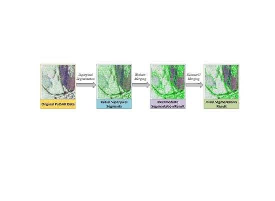
3. Methodology
3.1. Wishart-Merging Stage
3.2. KummerU-Merging Stage
| Algorithm 1: KUMS iterative merging. | |
| Begin | |
| 1. | For each pair of adjacent regions, calculate the KummerU energy loss , the edge penalty function , and the homogeneity penalty Fh, then obtain the merging criterion SCij, according to Equation (27) |
| 2. | Find the minimum SCij, and merge the corresponding adjacent regions. |
| 3. | Update the region adjacency graph RAG, and re-calculate the merging criterion SCij which is related to the newly merged region, and continue from Step 2. |
| 4. | Determine the appropriate number of the regions based on the L-method, and the final segmentation result is obtained accordingly. |
| End | |
3.3. Procedure of the Proposed Method
4. Experimental Results and Analysis
4.1. Datasets Description and Parameter Settings
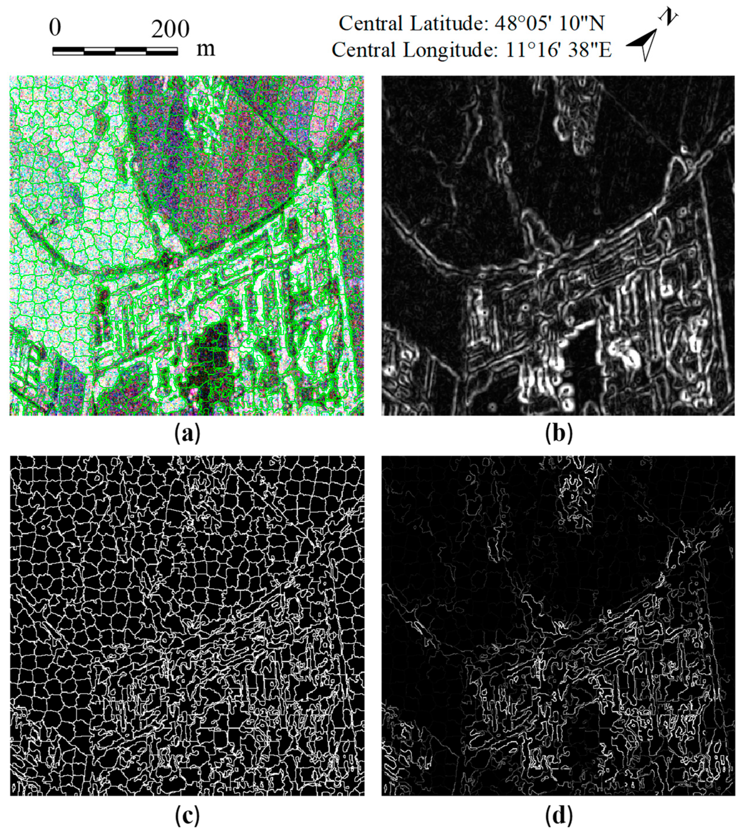
4.2. Segmentation Results of ESAR Data
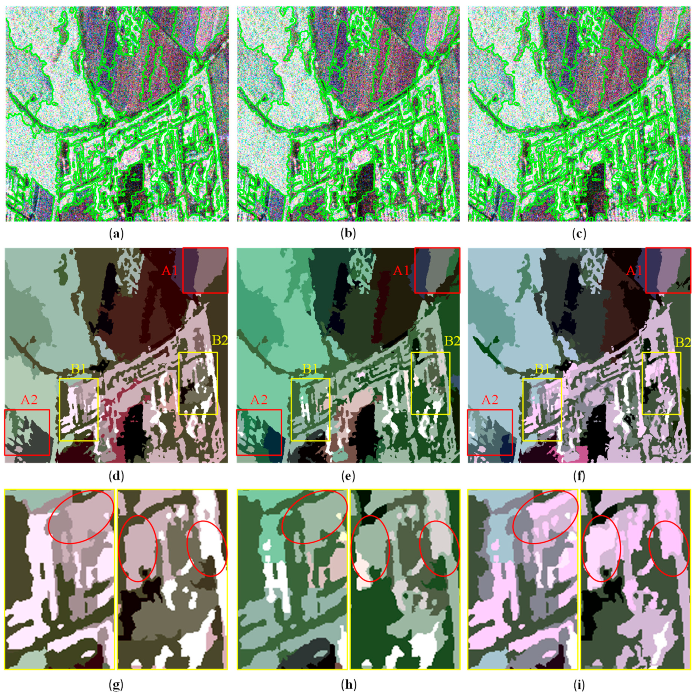
4.3. Segmentation Results of EMISAR Data
5. Conclusions
Author Contributions
Funding
Acknowledgments
Conflicts of Interest
References
- Chen, J.; Chen, Y.; An, W.; Cui, Y.; Yang, J. Nonlocal Filtering for Polarimetric SAR Data: A Pretest Approach. IEEE Trans. Geosci. Remote Sens. 2011, 49, 1744–1754. [Google Scholar] [CrossRef]
- Wang, W.; Xiang, D.; Zhang, J.; Wan, J. Integrating Contextual Information With H/α Decomposition for PolSAR Data Classification. IEEE Geosci. Remote Sens. Lett. 2016, 13, 2034–2038. [Google Scholar] [CrossRef]
- Niu, X.; Ban, Y. Multi-temporal RADARSAT-2 polarimetric SAR data for urban land-cover classification using an object-based support vector machine and a rule-based approach. Int. J. Remote Sens. 2013, 34, 1–26. [Google Scholar] [CrossRef]
- Wu, Y.; Ji, K.; Yu, W.; Su, Y. Region-based classification of polarimetric SAR images using Wishart MRF. IEEE Geosci. Remote Sens. Lett. 2008, 5, 668–672. [Google Scholar] [CrossRef]
- Xu, Q.; Chen, Q.; Yang, S.; Liu, X. Superpixel-Based Classification Using K Distribution and Spatial Context for Polarimetric SAR Images. Remote Sens. 2016, 8, 619. [Google Scholar] [CrossRef]
- Liu, W.; Yang, J.; Li, P.; Han, Y.; Zhao, J.; Shi, H. A Novel Object-Based Supervised Classification Method with Active Learning and Random Forest for PolSAR Imagery. Remote Sens. 2018, 10, 1092. [Google Scholar] [CrossRef]
- Qi, Z.; Yeh, A.G.-O.; Li, X.; Lin, Z. A novel algorithm for land use and land cover classification using RADARSAT-2 polarimetric SAR data. Remote Sens. Environ. 2012, 118, 21–39. [Google Scholar] [CrossRef]
- Yang, W.; Yang, X.; Yan, T.; Song, H.; Xia, G.S. Region-Based Change Detection for Polarimetric SAR Images Using Wishart Mixture Models. IEEE Trans. Geosci. Remote Sens. 2016, 54, 6746–6756. [Google Scholar] [CrossRef]
- Ghanbari, M.; Akbari, V. Unsupervised Change Detection in Polarimetric SAR Data With the Hotelling-Lawley Trace Statistic and Minimum-Error Thresholding. IEEE J. Sel. Top. Appl. Earth Obs. Remote Sens. 2018, 11, 4551–4562. [Google Scholar] [CrossRef]
- Wang, Y.; Liu, H. PolSAR Ship Detection Based on Superpixel-Level Scattering Mechanism Distribution Features. IEEE Geosci. Remote Sens. Lett. 2015, 12, 1780–1784. [Google Scholar] [CrossRef]
- Ran, L.; Liu, Z.; Li, T.; Xie, R.; Zhang, L. An Adaptive Fast Factorized Back-Projection Algorithm With Integrated Target Detection Technique for High-Resolution and High-Squint Spotlight SAR Imagery. IEEE J. Sel. Top. Appl. Earth Obs. Remote Sens. 2018, 11, 171–183. [Google Scholar] [CrossRef]
- Mahdianpari, M.; Salehi, B.; Mohammadimanesh, F.; Motagh, M. Random forest wetland classification using ALOS-2 L-band, RADARSAT-2 C-band, and TerraSAR-X imagery. ISPRS J. Photogramm. Remote Sens. 2017, 130, 13–31. [Google Scholar] [CrossRef]
- Mohammadimanesh, F.; Salehi, B.; Mahdianpari, M.; Motagh, M.; Brisco, B. An efficient feature optimization for wetland mapping by synergistic use of SAR intensity, interferometry, and polarimetry data. Int. J. Appl. Earth Obs. Geoinf. 2018, 73, 450–462. [Google Scholar] [CrossRef]
- Wang, Y.; Han, C.; Tupin, F. PolSAR Data Segmentation by Combining Tensor Space Cluster Analysis and Markovian Framework. IEEE Geosci. Remote Sens. Lett. 2010, 7, 210–214. [Google Scholar] [CrossRef]
- Cao, F.; Hong, W.; Wu, Y.; Pottier, E. An unsupervised segmentation with an adaptive number of clusters using the SPAN/H/α/A space and the complex Wishart clustering for fully polarimetric SAR data analysis. IEEE Trans. Geosci. Remote Sens. 2007, 45, 3454–3467. [Google Scholar] [CrossRef]
- Yu, P.; Qin, A.; Clausi, D.A. Unsupervised polarimetric SAR image segmentation and classification using region growing with edge penalty. IEEE Trans. Geosci. Remote Sens. 2012, 50, 1302–1317. [Google Scholar] [CrossRef]
- Lang, F.; Yang, J.; Li, D.; Zhao, L.; Shi, L. Polarimetric SAR image segmentation using statistical region merging. IEEE Geosci. Remote Sens. Lett. 2014, 11, 509–513. [Google Scholar] [CrossRef]
- Alonso-González, A.; López-Martínez, C.; Salembier, P. Filtering and segmentation of polarimetric SAR data based on binary partition trees. IEEE Trans. Geosci. Remote Sens. 2012, 50, 593–605. [Google Scholar] [CrossRef]
- Salembier, P.; Foucher, S. Optimum Graph Cuts for Pruning Binary Partition Trees of Polarimetric SAR Images. IEEE Trans. Geosci. Remote Sens. 2016, 54, 5493–5502. [Google Scholar] [CrossRef]
- Liu, B.; Zenghui, Z.; Xingzhao, L.; Wenxian, Y. Representation and Spatially Adaptive Segmentation for PolSAR Images Based on Wedgelet Analysis. IEEE Trans. Geosci. Remote Sens. 2015, 53, 4797–4809. [Google Scholar] [CrossRef]
- Ersahin, K.; Cumming, I.G.; Ward, R.K. Segmentation and classification of polarimetric SAR data using spectral graph partitioning. IEEE Trans. Geosci. Remote Sens. 2010, 48, 164–174. [Google Scholar] [CrossRef]
- Lee, J.; Pottier, E. Polarimetric Radar Imaging: From Basics to Applications; CRC Press: Boca Raton, FL, USA, 2009. [Google Scholar]
- Akbari, V.; Doulgeris, A.P.; Moser, G.; Eltoft, T.; Anfinsen, S.N.; Serpico, S.B. A Textural-Contextual Model for Unsupervised Segmentation of Multipolarization Synthetic Aperture Radar Images. IEEE Trans. Geosci. Remote Sens. 2013, 51, 2442–2453. [Google Scholar] [CrossRef]
- Bombrun, L.; Beaulieu, J.M. Fisher distribution for texture modeling of Polarimetric SAR data. IEEE Geosci. Remote Sens. Lett. 2008, 5, 512–516. [Google Scholar] [CrossRef]
- Deng, X.; López-Martínez, C.; Chen, J.; Han, P. Statistical Modeling of Polarimetric SAR Data: A Survey and Challenges. Remote Sens. 2017, 9, 348. [Google Scholar] [CrossRef]
- Doulgeris, A.P.; Anfinsen, S.N.; Eltoft, T. Classification with a Non-Gaussian model for PolSAR Data. IEEE Trans. Geosci. Remote Sens. 2008, 46, 2999–3009. [Google Scholar] [CrossRef]
- Freitas, C.C.; Frery, A.C.; Correia, A.H. The polarimetric G distribution for SAR data analysis. Environmetrics 2005, 16, 13–31. [Google Scholar] [CrossRef]
- Doulgeris, A.P. An Automatic U-Distribution and Markov Random Field Segmentation Algorithm for PolSAR Images. IEEE Trans. Geosci. Remote Sens. 2015, 53, 1819–1827. [Google Scholar] [CrossRef]
- Bombrun, L.; Vasile, G.; Gay, M.; Totir, F. Hierarchical segmentation of polarimetric SAR images using heterogeneous clutter models. IEEE Trans. Geosci. Remote Sens. 2011, 49, 726–737. [Google Scholar] [CrossRef]
- Beaulieu, J.M.; Touzi, R. Segmentation of textured polarimetric SAR scenes by likelihood approximation. IEEE Trans. Geosci. Remote Sens. 2004, 42, 2063–2072. [Google Scholar] [CrossRef]
- Qin, F.; Guo, J.; Lang, F. Superpixel segmentation for polarimetric SAR imagery using local iterative clustering. IEEE Geosci. Remote Sens. Lett. 2015, 12, 13–17. [Google Scholar] [CrossRef]
- Xiang, D.; Ban, Y.; Wang, W.; Su, Y. Adaptive Superpixel Generation for Polarimetric SAR Images With Local Iterative Clustering and SIRV Model. IEEE Trans. Geosci. Remote Sens. 2017, 55, 3115–3131. [Google Scholar] [CrossRef]
- Lang, F.; Yang, J.; Yan, S.; Qin, F. Superpixel Segmentation of Polarimetric Synthetic Aperture Radar (SAR) Images Based on Generalized Mean Shift. Remote Sens. 2018, 10, 1592. [Google Scholar] [CrossRef]
- Song, H.; Yang, W.; Bai, Y.; Xu, X. Unsupervised classification of polarimetric SAR imagery using large-scale spectral clustering with spatial constraints. Int. J. Remote Sens. 2015, 36, 2816–2830. [Google Scholar] [CrossRef]
- Anfinsen, S.N.; Eltoft, T. Application of the Matrix-Variate Mellin Transform to Analysis of Polarimetric Radar Images. IEEE Trans. Geosci. Remote Sens. 2011, 49, 2281–2295. [Google Scholar] [CrossRef]
- Nicolas, J.-M. Application de la transformée de Mellin: Étude des lois statistiques de l’imagerie cohérente. Rapport de Recherche 2006, 2006, D010. [Google Scholar]
- Anfinsen, S.N.; Doulgeris, A.P.; Eltoft, T. Goodness-of-Fit Tests for Multi-look Polarimetric Radar Data Based on the Mellin Transform. IEEE Trans. Geosci. Remote Sens. 2011, 49, 2764–2781. [Google Scholar] [CrossRef]
- Wang, W.; Xiang, D.; Ban, Y.; Zhang, J.; Wan, J. Superpixel Segmentation of Polarimetric SAR Images Based on Integrated Distance Measure and Entropy Rate Method. IEEE J. Sel. Top. Appl. Earth Obs. Remote Sens. 2017, 10, 4045–4058. [Google Scholar] [CrossRef]
- Liu, M.Y.; Tuzel, O.; Ramalingam, S.; Chellappa, R. Entropy rate superpixel segmentation. In Proceedings of the CVPR 2011, Colorado Springs, CO, USA, 20–25 June 2011; pp. 2097–2104. [Google Scholar]
- Qin, X.; Zhou, S.; Zou, H. SAR Image Segmentation via Hierarchical Region Merging and Edge Evolving With Generalized Gamma Distribution. IEEE Geosci. Remote Sens. Lett. 2014, 11, 1742–1746. [Google Scholar] [CrossRef]
- Yu, Q.; Clausi, D.A. IRGS: Image Segmentation Using Edge Penalties and Region Growing. IEEE Trans. Pattern Anal. Mach. Intell. 2008, 30, 2126–2139. [Google Scholar] [CrossRef]
- Xiang, D.; Ban, Y.; Wang, W.; Tang, T.; Su, Y. Edge Detector for Polarimetric SAR Images Using SIRV Model and Gauss-Shaped Filter. IEEE Geosci. Remote Sens. Lett. 2016, 13, 1661–1665. [Google Scholar] [CrossRef]
- Yang, S.; Chen, Q.; Yuan, X.; Liu, X. Adaptive Coherency Matrix Estimation for Polarimetric SAR Imagery Based on Local Heterogeneity Coefficients. IEEE Trans. Geosci. Remote Sens. 2016, 54, 6732–6745. [Google Scholar] [CrossRef]
- Touzi, R. A review of speckle filtering in the context of estimation theory. IEEE Trans. Geosci. Remote Sens. 2002, 40, 2392–2404. [Google Scholar] [CrossRef]
- Salvador, S.; Chan, P. Determining the number of clusters/segments in hierarchical clustering/segmentation algorithms. In Proceedings of the 16th IEEE International Conference on Tools with Artificial Intelligence, Boca Raton, FL, USA, 15–17 November 2004; pp. 576–584. [Google Scholar]
- Martin, D.R.; Fowlkes, C.C.; Malik, J. Learning to detect natural image boundaries using local brightness, color, and texture cues. IEEE Trans. Pattern Anal. Mach. Intell. 2004, 26, 530–549. [Google Scholar] [CrossRef] [PubMed] [Green Version]


| IM-Wishart | IM-KummerU | The Proposed Method | ||
|---|---|---|---|---|
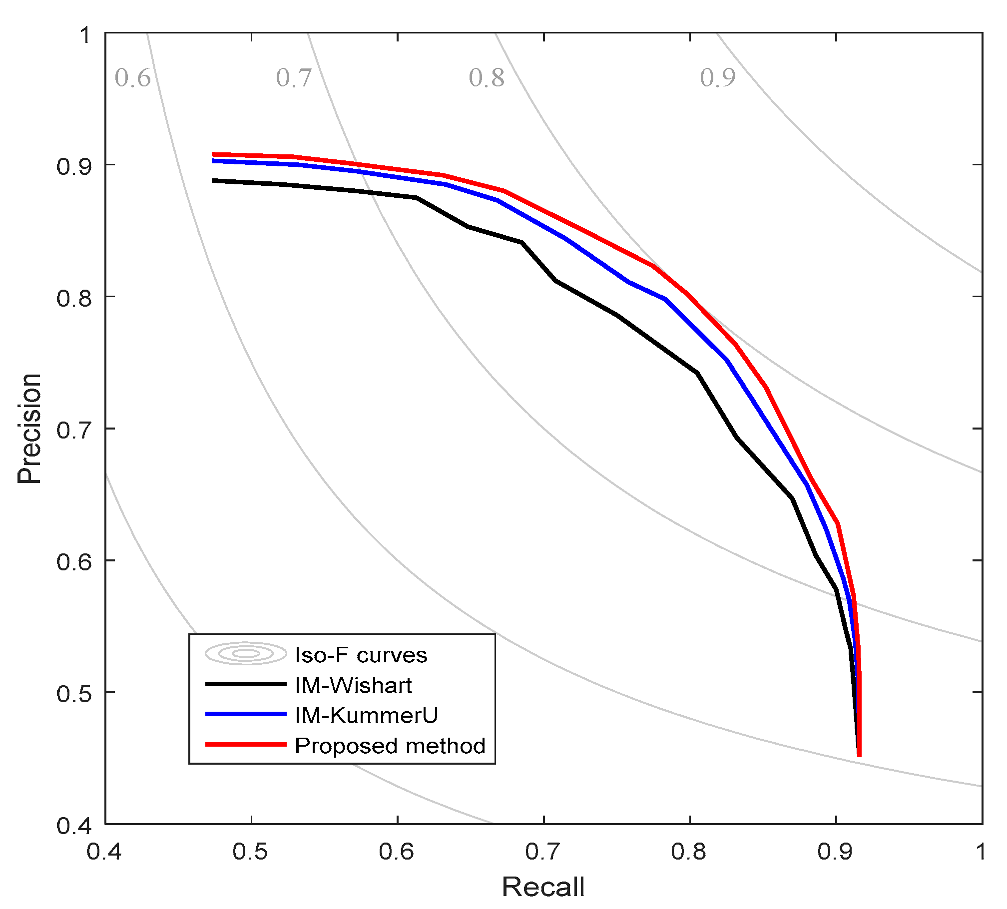
| ESAR | Precision | 0.772 | 0.794 | 0.8 |
| Recall | 0.758 | 0.788 | 0.8 | |
| F-measure | 0.765 | 0.791 | 0.8 | |
| EMISAR | Precision | 0.768 | 0.797 | 0.81 |
| Recall | 0.76 | 0.787 | 0.804 | |
| F-measure | 0.764 | 0.792 | 0.807 | |
| IM-Wishart | IM-KummerU | The Proposed Method | |||
|---|---|---|---|---|---|
| WMS | KUMS | Total | |||
| ESAR | 337.5 | 703.8 | 2.7 | 256.2 | 258.9 |
| EMISAR | 453.4 | 914.6 | 3.5 | 371.8 | 375.3 |
© 2019 by the authors. Licensee MDPI, Basel, Switzerland. This article is an open access article distributed under the terms and conditions of the Creative Commons Attribution (CC BY) license (http://creativecommons.org/licenses/by/4.0/).
Share and Cite
Wang, W.; Xiang, D.; Ban, Y.; Zhang, J.; Wan, J. Superpixel-Based Segmentation of Polarimetric SAR Images through Two-Stage Merging. Remote Sens. 2019, 11, 402. https://doi.org/10.3390/rs11040402
Wang W, Xiang D, Ban Y, Zhang J, Wan J. Superpixel-Based Segmentation of Polarimetric SAR Images through Two-Stage Merging. Remote Sensing. 2019; 11(4):402. https://doi.org/10.3390/rs11040402
Chicago/Turabian StyleWang, Wei, Deliang Xiang, Yifang Ban, Jun Zhang, and Jianwei Wan. 2019. "Superpixel-Based Segmentation of Polarimetric SAR Images through Two-Stage Merging" Remote Sensing 11, no. 4: 402. https://doi.org/10.3390/rs11040402