Article

Active Learning for Recognition of Shipwreck Target in Side-Scan Sonar Image

1
NanJing Research Institute of Surveying, Mapping & Geotechnical Investigation, Co. Ltd., Nanjing 210019, China
2
School of Geomatics and Marine Information, Huaihai Institute of Technology, 59 Cangwu Road, Lianyungang 222005, China
*
Author to whom correspondence should be addressed.
Remote Sens. 2019, 11(3), 243; https://doi.org/10.3390/rs11030243
Submission received: 25 December 2018 / Revised: 21 January 2019 / Accepted: 21 January 2019 / Published: 24 January 2019
(This article belongs to the Special Issue Remote Sensing of Target Detection in Marine Environment)

Abstract

:
In order to realize the automatic and accurate recognition of shipwreck targets in side-scan sonar (SSS) waterfall images, a pipeline that contains feature extraction, selection, and shipwreck recognition, an AdaBoost model was constructed by sample images. Shipwreck targets are detected quickly by a nonlinear matching model, and a shipwreck recognition in SSS waterfall images are given, and according to a wide set of combinations of different types of these individual procedures, the model is able to recognize the shipwrecks accurately. Firstly, two feature-extraction methods suitable for recognizing SSS shipwreck targets from natural sea bottom images were studied. In addition to these two typical features, some commonly used features were extracted and combined as comprehensive features to characterize shipwrecks from various feature spaces. Based on Independent Component Analysis (ICA), the preferred features were selected from the comprehensive features, which avoid dimension disaster and improved the correct recognition rate. Then, the Gentle AdaBoost algorithm was studied and used for constructing the shipwreck target recognition model using sample images. Finally, a shipwreck target recognition process for the SSS waterfall image was given, and the process contains shipwreck target fast detection by a nonlinear matching model and accurate recognition by the Gentle AdaBoost recognition model. The results show that the correct recognition rate of the model for the sample image is 97.44%, while the false positive rate is 3.13% and the missing detection rate is 0. This study of a measured SSS waterfall image confirms the correctness of the recognition process and model.

1. Introduction

Side-scan sonar (SSS) is often applied to ocean engineering for obtaining high-resolution seabed images and detecting underwater targets such as aircrafts, shipwrecks, torpedoes, mine-like objects, etc. [1,2,3,4,5,6]. In practice, target detection and recognition from SSS images are mostly based on manual interpretation, and thus its efficiency and accuracy are significantly affected by the experience of the sonar map reader. Some commercial SSS image processing software, such as Triton, Hips and SonerWeb, all provide a manual target detection function [7]. Therefore, automatic and accurate target detection and recognition methods need to be studied in-depth. For target recognition, the general processes are feature extraction, feature selection, the construction of the target recognition model and the application of the model. Dobeck et al. (1997) proposed an advanced mine-detection and classification (AMDAC) algorithm for sonar images which was comprised of four steps: (1) Image enhancement; (2) mine detection; (3) feature extraction and optimal feature selection; and (4) mine classification. In step (3), 45 kinds of features, such as shape and intensity features of the target, were extracted and used for sea mine recognition [8]. Dobeck (2000) proposed a combination of multiple classifiers to construct a comprehensive recognition model which effectively improved the correct recognition rate of the sea mines targets [9]. Reed et al. (2003) extracted features based on the frequency domain of images to complete the recognition of sea mines from a sand sea bottom image [10]. Langner et al. (2009) used a probabilistic neural network (PNN) to recognize underwater mine-like targets [11]. Isaacs (2015) found that features were generated on geometric moments in the imaging domain and performed a recognition process using an Ada-boosted decision tree classifier for underwater unexploded ordnance (UXO) remediation [12]. Guo et al. (2002) achieved the recognition of underwater small targets with shape parameters that were spherical, circular, etc., based on fuzzy clustering, and extracted shape features such as horizontal, height characteristic lines of the target image for target recognition; horizontal, height lines were calculated using the contour information of the shadow areas for a target [13]. Wang (2005) extracted the gray and moment invariant features of a simulated target image having a certain shape parameter and achieved target recognition based on the radial basis artificial neural network model [14]. Yang et al. (2006) studied an SSS image object recognition method using a simulated man-made target image based on grayscale histogram and geometric features [15]. Ma (2007) extracted shape and fractal dimension from an SSS target image and used a back propagation (BP) neural network to achieve the recognition of an underwater mine-like object [16]. Tang (2009) extracted texture features of an SSS image based on multi-resolution analysis, and used a BP neural network to recognize underwater simulated targets [17].
There are many kinds of feature extraction methods and recognition models used for SSS image target recognition that can achieve high correct recognition rate for certain different targets, with most research aimed at mine-like objects. All of these methods have been used to analyze SSS sample images [10,11,12,13,14,15,16,17], although not for the SSS whole waterfall image. What happens when combining some of these features as a comprehensive dataset for target recognition remains unclear.
Increased marine activities have led to frequent underwater shipwreck accidents, causing enormous casualties and economic losses. The accurate detection of shipwreck targets is the premise for underwater rescue. However, few studies have aimed to perform shipwreck target recognition. It is still necessary to conduct further research to find more suitable texture feature extraction methods for shipwreck target recognition, especially when the shape and gray features are difficult to extract, which is caused by a wreck being tilted, broken and covered by sediments, etc. It is also necessary to obtain the optimal feature if some of these features are combined as a comprehensive feature set, and to find the optimal recognition model construction algorithm which can be applied to SSS waterfall images obtained from complex marine noise.
The shipwreck target in SSS waterfall images can be recognized when the recognition model is constructed, but it is very time consuming if the feature extraction, selection and target recognition processes are applied in every moving window of the SSS waterfall image. Dobeck gave a general step for target detection and classification in SSS waterfall images [8,9], however the algorithms used in the literature are outdated. In-depth study is required to determine how to better use the recognition model in SSS waterfall images with large data sizes.
For this reason, this paper took a man-made shipwreck target as the research object and aimed to solve the aforementioned problems in SSS shipwreck recognition. The shipwreck recognition process is given to achieve the goal of automatic and accurate shipwreck recognition in SSS waterfall images. This process consists of two basic steps: Fast detection and precise recognition.
The remainder of this paper is organized as follows. Section 2 details the typical features of the man-made shipwreck target, introduces the methods of feature dimensionality reduction and aims to solve the problems of feature extraction and selection; Section 3 introduces the widely used recognition models, analyses the model which is suitable for SSS image shipwreck target recognition, gives the flow chart of shipwreck target recognition process for SSS waterfall image and aims to solve the problems of constructing a robust shipwreck recognition model and applying the model in SSS waterfall image which has a large dataset; Section 4 presents the experimental results; Section 5 discusses several issues affecting the results of the experiment and in Section 6 some conclusions are drawn.

2. Feature Extraction and Selection Methods

Theoretically and intuitively, except for the shape parameter, man-made (iron, wooden, etc.) targets are different from natural sea bottom (sand, rock, etc.) in materials and under the representation of some textural feature values; these textural features are defined as typical features, and two typical features are introduced as follows.

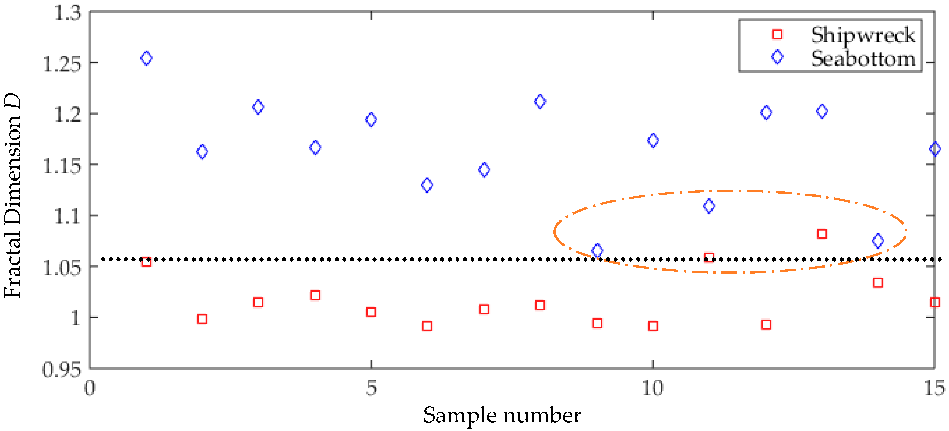
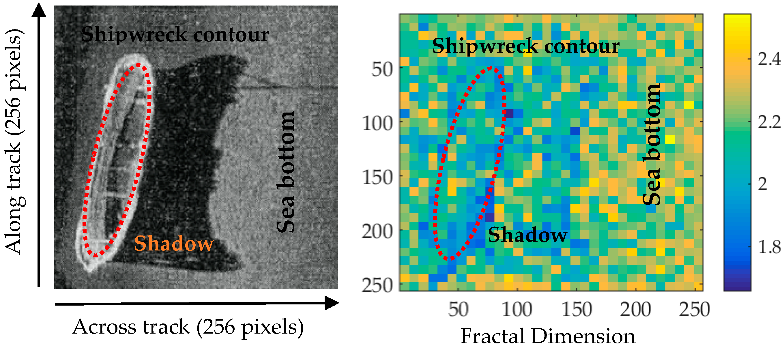
2.1. Fractal Geometry

Fractal geometry is a useful technique for analysis of digital images in terms of its roughness. Roughness of digital image can be estimated from the overall distribution of intensity points based on the concept of self-similarity. From the property of self-similarity, the fractal is normally an irregular geometric structure that can be broken into smaller pieces; each of the smaller pieces are related to the original and similar to the original. A surrounded set X in Euclidean n-space is self-similar if X is the unification of Nr distinct (non-overlapping) copies of r itself, scaled up or down by a factor of r [18]. The fractal dimension D of X is given by:
D = log ( N r ) log ( 1 / r )
where Nr represents the distinct copies of X of the scale of reduction factor r. Differential box-counting (DBC) is a commonly used algorithm to estimate surface roughness of gray scale image and its details are as follows.
A two-dimensional SSS image actually has two calculable fractal dimensions, one for each of its two topological dimensions. The two fractal dimensions correspond to the average variation in texture, or pixel intensity, in the along and across-track directions. And the fractal dimension D must meet the condition: 1 ≤ D ≤ 2, where 1 indicates flat or regular surface, 2 indicates extremely corrugated one. Although an image representing a physical surface has a third topological dimension, an image maps the surface with a two-dimension snapshot that reduces three-dimensional geographical information into a single pixel intensity for each image portion [19].
The DBC algorithm considers an image of size M × M which has broken down of size L × L, where L represents the box size of integer type of range from 2 to M/2. The image can be represented in 3-Dimensional spatial space, where (x, y) represents 2-Dimension spatial space and a 3rd coordinate Z represents gray level G. In the next step, partitioning the x, y plane into grids of size L × L, each grid contains column of boxes of size L × L × L′, where L′ represents height of the box and can be evaluated as L′ = L × G/M and the reduction factor r can be computed as M/L. The minimum and maximum gray level of input images fall into respectively Mk th and Ml th, then nr (i, j) can be evaluated as follows [18]:
n r ( i , j ) = M l M k + 1
Finally, Nr can be computed by taking contribution from each grid of scale r based on:
N r = i , j n r ( i , j )
Different types of objects in the natural world generally have different values of D. There is a certain correspondence between the fractal dimension and the gray level of an image. D is matched for the surface roughness of the object, and different textural images have a large difference in roughness [20]. A total of 30 different pieces of shipwreck and sea bottom SSS images were selected to calculate D. All of these images were selected from the data collected by ourselves in different areas in China with different SSS instruments. All of these 30 images had a size of 128 × 128 pixels. The sea bottom images were collected with different types of geological structures, such as sand, rock, etc. But these sea bottom images did not contain any man-made target, the results are shown in Figure 1.
It can be seen from Figure 1 that the fractal dimension value for SSS images of a shipwreck target are smaller than that of sea bottom image. There are only four samples that are difficult to distinguish. Therefore, fractal dimension can be used for object recognition, especially for distinguishing man-made shipwreck targets from natural sea bottom backgrounds for SSS images. In summary, the fractal dimension D is defined as the typical texture feature of SSS shipwreck target.

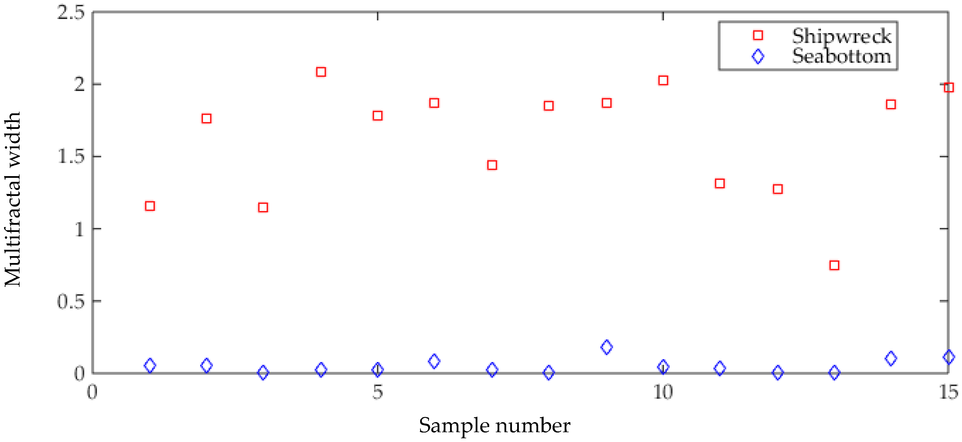
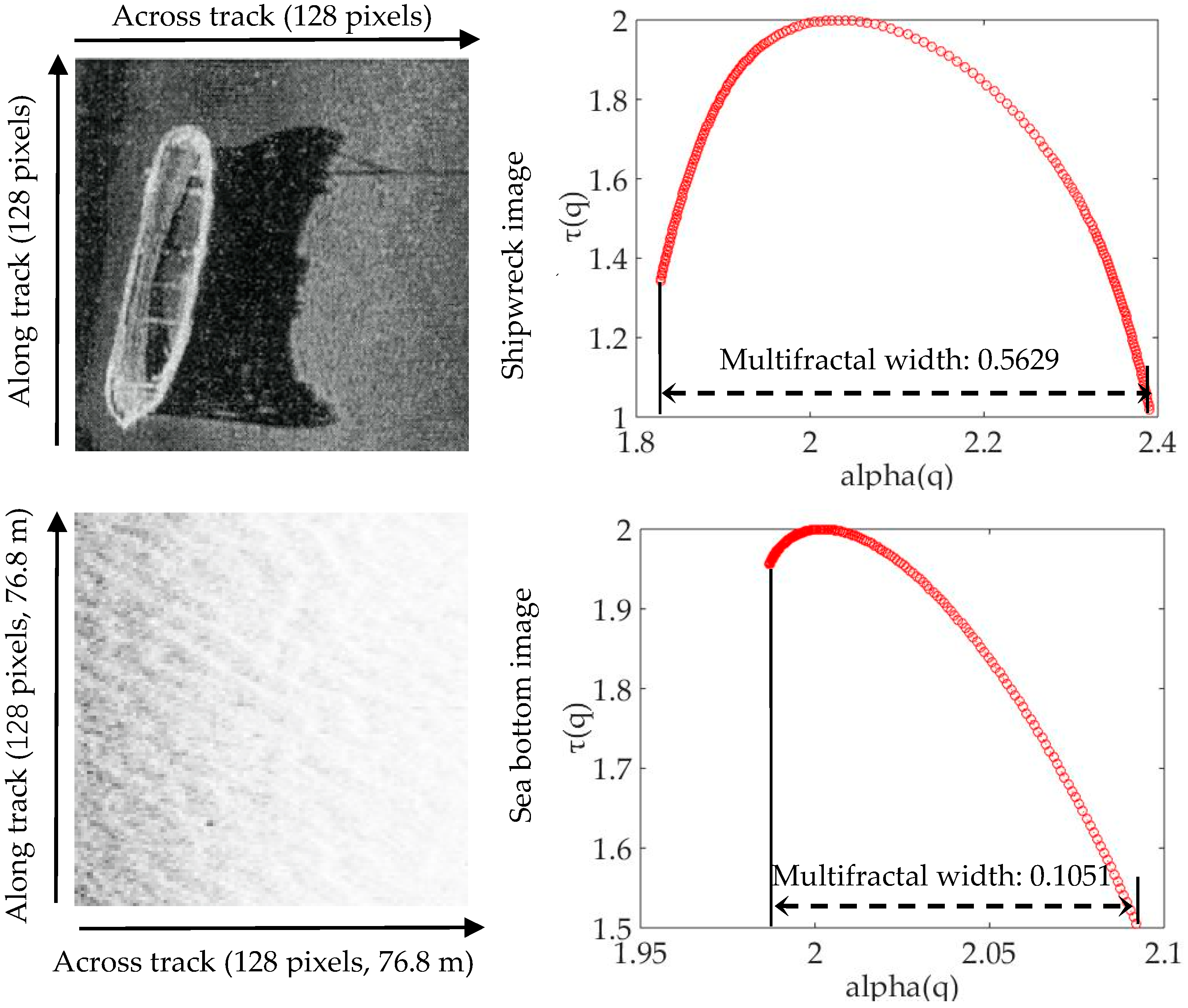
2.2. Multifractal Features

Fractal feature is useful for describing man-made shipwreck targets from sea bottom images. However, some studies show that images of many different textures are similar in their calculated fractal values that are not visually identical; the experiments shown in Figure 1 also demonstrate this problem [21]. The reason for this is that the fractal dimension can only describe those fractal objects with ideal self-similarities, and many real-world textures do not satisfy this condition. In order to obtain a more detailed description of a fractal object, it is necessary to add parameters that can characterize different fractal subsets. Therefore, the multifractal theory is introduced.
A formula, named “multifractal formalism” was established in order to compute the multifractal [22]. The multifractal formalism was then defined by:
D ( h ) = inf q ( q · h τ ( q ) + c )
where q is a real number, c is a constant and τ(q) is called the partition function.
A multifractal structure can be considered as a superposition of homogeneous monofractal structures. Let us consider the set E(h) of Holder exponents h of particles with values in the interval [h, h + Dh]. F(h) is defined as the fractal dimension of the set E(h), which has a monofractal structure. The pairs (q, s(q)) and (h, F(h)) are linked by the Legendre transform:
τ ( q ) = q · κ ( q ) F ( h ) κ ( q ) α ( q ) = d τ ( q ) d q
where α is an approximation of the Holder coefficient h. For a multifractal structure, the dimensions Dq are decreasing functions of q, and hF(h) is a convex function whose maximum corresponds to the Hausdorff dimension Dh. The width between α(q)min and α(q)max was defined as the multifractal width and used in the experiments.
Islam et al. introduced the details of the calculation of multifractals [21]. As in fractal feature estimation, many methods exist to approximately calculate the multifractal, and the box-counting method based on the same principles for fractal dimension is also used for calculating multifractals.
The multifractal width feature was calculated by the same images used in Figure 1, and the results are shown in Figure 2. It can be seen from Figure 2 that the multifractal widths for SSS image of shipwreck targets are all larger than that of sea bottom image, and the multifractal width can be defined as the typical textural feature for recognizing SSS shipwreck target.

2.3. Feature Selection Methods

The possible typical features of the shipwreck image are described above. However, there are other typical textural features that can be used for SSS man-made shipwreck recognition. Considering the complex marine environment and the noise of underwater SSS images, it is still necessary to extract a large number of other features to increase the dimension of shipwreck features and enrich the expression of shipwreck features. However, in actual applications, selecting more kinds of features is not necessarily better. Some researchers have found that if the features’ dimension is larger, the robustness of the recognition classifier will be reduced [23]. Moreover, the increase of the dimensionality of the features will lead to the “dimensionality disaster”, which further affects the calculation efficiency.
Therefore, another important task before constructing the recognition model is to extract a small number of robust features from a large number of features, that is, feature dimension reduction or optimal feature selection. The reliability of the recognition results sometimes depends on the cohesion and inter-class variability of the features in the classification space [24]. Principal Component Analysis (PCA) and Independent Component Analysis (ICA) are the methods used in this manuscript.
PCA involves seeking for orthogonal projections that best explain the variance of a feature set and is suitable for those data with Gaussian distribution. However, due to the complex marine environment, the data may not necessarily be Gaussian. SSS images were obtained by different devices under the influence of complex marine environment and were used as the sample database. The extracted features are often independent. The background is dominant in the SSS image, and the target may only be a secondary component. Thus, PCA is not suitable for SSS image optimal feature extraction.
ICA involves seeking random projections that maximize higher-order statistical criteria, such as absolute normalized kurtosis, a fourth order statistic, and non-Gaussian problems. ICA assumes that the observed multivariate data are linear or non-linear mixtures of some unknown non-Gaussian and mutually independent latent variables, called independent components, which are attempted to be determined [25]. ICA can also obtain better data dimensionality reducing results and achieve optimal feature extraction, resulting in small sample sets.
In summary, ICA can be used as the optimal feature selection algorithm for the SSS image, and to reduce the feature dimensionality and optimize the texture features of the shipwreck target.

3. Recognition Models

The shipwreck recognition model can be constructed by the preferred selected features obtained above. We used AdaBoost, k-Nearest-Neighbors (kNN), random forests (RFs) and Support Vector Machine (SVM) algorithms in the experiment to construct the model. The basic principles of each model are briefly introduced, and their characteristics are analyzed as follows.

3.1. Recognition Models

1. k-Nearest Neighbors
kNN is a simple but effective method for classification problem. The flowchart of the kNN algorithm is shown in Table 1.
The major drawbacks with respect to kNN are: (1) Its low efficiency; the fact that it is a lazy learning method prohibits its use in many applications; and (2) its dependency on the selection of a “good value” for k and on the influence of the test samples, such as there is only a few samples [26].
2. Random Forests (RFs)
The RFs are a combination of many decision trees that are created using bootstrapping technique coming from the learning dataset samples of the predictors and choosing randomly at each node. The principle of RFs is performed with respect to classification and regression trees (CART) model strategy. The RFs algorithm estimates the importance of the variables by comparing the prediction error with Out-Of-Bag (OOB) data term.
Advantages of RFs compared to other statistical classifiers include: (1) Very high classification accuracy; (2) a novel method of determining variable importance; (3) the ability to model complex interactions among predictor variables; (4) flexibility to perform several types of statistical data analysis; and (5) an algorithm for imputing missing values. RFs will be fitted over for some noisy classification or regression problems [27].
3. Support Vector Machine
The mechanism of SVM is to find an optimal class hyperplane that meets the classification requirements, which enables the hyperplane to ensure the accuracy of the classification and maximize the blank area on both sides of the hyperplane.
If given training samples (xi, yi), i = 1, 2, …, m, x∈Rn, and when y∈{ ± 1}, this is a two-type data classification problem, m is the sample number. The hyperplane can be defined as (w·x) + b = 0 for making the classification plane correctly classify all samples, and it is required to satisfy the following constraints:
y i [ ( w · x i ) + b ] 1 i = 1 , 2 , , m
where w represents a weight matrix, and x represents the sample feature matrix. It can be calculated that the classification interval is 2 w , so the problem of constructing the hyperplanes translates into calculating:
min ϕ ( w ) = 1 2 w 2 = 1 2 ( w · w )
To solve this constraint optimization problem, the Lagrange function is introduced:
L ( w , b , a ) = 1 2 w a ( y ( ( w · x ) + b ) 1 )
where ai > 0 is the Lagrange multiplier, the solution to the optimization problem meets the partial derivative of w, and b is 0. Turn the quadratic programming (QP) question into the corresponding dual problem:
max Q ( a ) = j = 1 m a j 1 2 i = 1 m j = 1 m a i a j y i y j ( x i x j ) s . t . j = 1 m a j y j = 0    j = 1 , 2 , , m ,    a j 0
Then the optimal solution of a* can be calculated as (a1*, a2*, …, am*)T, and the optimal solution of w* and b* can be calculated as:
w * = j = 1 m a j * y j x j b * = y i j = 1 m y j a j * ( x j · x i )
where j∈{j|aj* > 0}. Thus, the optimal hyperplane is (w*·x) + b* = 0, and the optimal classification function is:
f ( x ) = sgn { ( w * · x ) + b * } = sgn { ( j = 1 m a j * y j ( x j x i ) ) + b * } , x R n
SVM is a better option to solve problems for fewer training samples, higher feature dimensionality and linear inseparability. However, the drawback is that SVM does not consider some latent variables [28].
4. AdaBoost
Given a set of training samples, AdaBoost maintains a weight distribution, W, over these samples. This distribution is initially set to be uniform, and AdaBoost repeatedly calls a component learn algorithm in a series of cycles, as shown in Algorithm 1.
Algorithm 1 The flowchart of the AdaBoost.
1. Input: a set of training samples with labels y, (x1, y1), (x2, y2), …, (xm, ym), x is the feature set, m is the sample number; a component learn algorithm; the number of cycles T.
2. Initialize: the weights of training samples: w 1 , j = 1 m , for j = 1, 2, …, m.
3. Do for t = 1, 2, …, T.
(1)
Use the Component Learn algorithm to train a component classifier, et, on the weighted training samples.
(2)
Calculate the training error of et: ε t = i = 1 m w i t ,   y i e t ( x i ) .
(3)
Set weight for the component classifier et: α t = ln ( 1 ε t ε t ) .
(4)
Update the weights of training samples: w t + 1 , i = w t , i exp ( a t y i e t ( x i ) ) Z t , t = 1 , 2 , , m ,    where , Z t = i = 1 m w t , i exp ( α t y i e t ( x i ) ) .
4. Output: H ( x ) = sgn ( t = 1 T a t e t ( x ) ) .
Many improvements have been made to AdaBoost, and many new forms have emerged. At present, Modest AdaBoost and Gentle AdaBoost are two commonly used algorithms. AdaBoost has the following advantages: (1) Higher recognition accuracy; (2) the component learning algorithm can be built in a variety of ways, and AdaBoost provides a framework; (3) the improved Gentle AdaBoost does not suffer from the problem of over-fitting [29]. Therefore, AdaBoost can be seen as a natural algorithm that proposes a fusion of multiple classifiers, and it has been shown that this multiple characteristic can improve the correct recognition rate for underwater targets [9].
Using the preferred selected features, different shipwreck recognition models can be constructed based on the above algorithms. As mentioned in the introduction, it is time consuming if the feature extraction and target recognition process are applied in every moving window in SSS waterfall image. By analyzing the mechanism of SSS measurement and the characteristics of the target in SSS image, a flow chart of the shipwreck target recognition in SSS waterfall image is given to achieve better application of the model, and is introduced as follows.

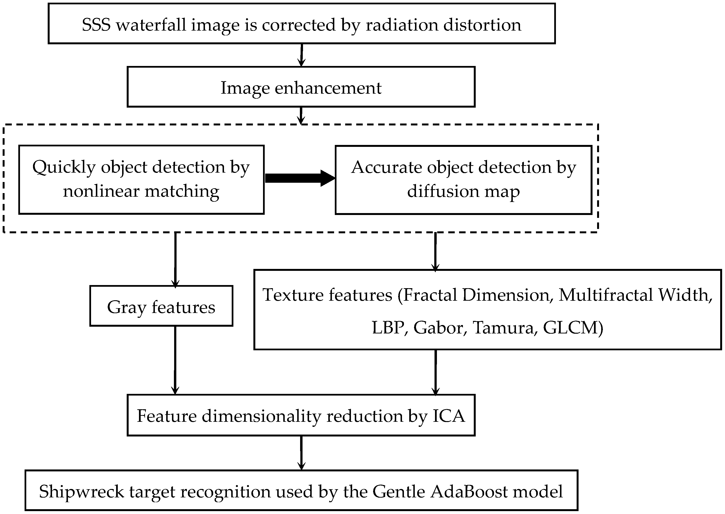
3.2. Flow Chart of the Shipwreck Target Recognition in SSS Waterfall Images

In SSS imaging, a sonar array is typically mounted on either side of a towfish or an autonomous underwater vehicle (AUV). Two fan-shaped beams are transmitted perpendicular to the towfish or AUV travel path, and starboard (stbd) and port SSS sea bottom images are formed through received beam forming. During the transmitting pulse, the receiving circuitry is switched off to prevent damage or saturation of the high-sensitivity amplifiers. After the completion of the transmitting pulse, the transducers are switched over to the receiving circuitry, and the continuous recording of the incoming acoustic signal begins. The signals scan a swath of the sea bottom from a point just below the towfish to a limited distance away from the line of travel (slant range) on both sides [30], and this forms a ping measurement. A series of pings can be obtained continuously in SSS measurements, and a waterfall image will finally be formed by these ping measurements, as shown in Figure 3. The water column image is formed due to the transmitting time of the acoustic wave through the water before the first reflected sound wave from the seabed.
Taking into account the efficiency and accuracy of shipwreck target recognition in SSS waterfall image which has a large dataset, and that the target may be visible in the water column image, a shipwreck target recognition process is given, the flow chat for which is shown in Figure 4. In order to ensure the effectiveness of feature extraction, the size of the detection image is selected to be the same as that of the sample image.

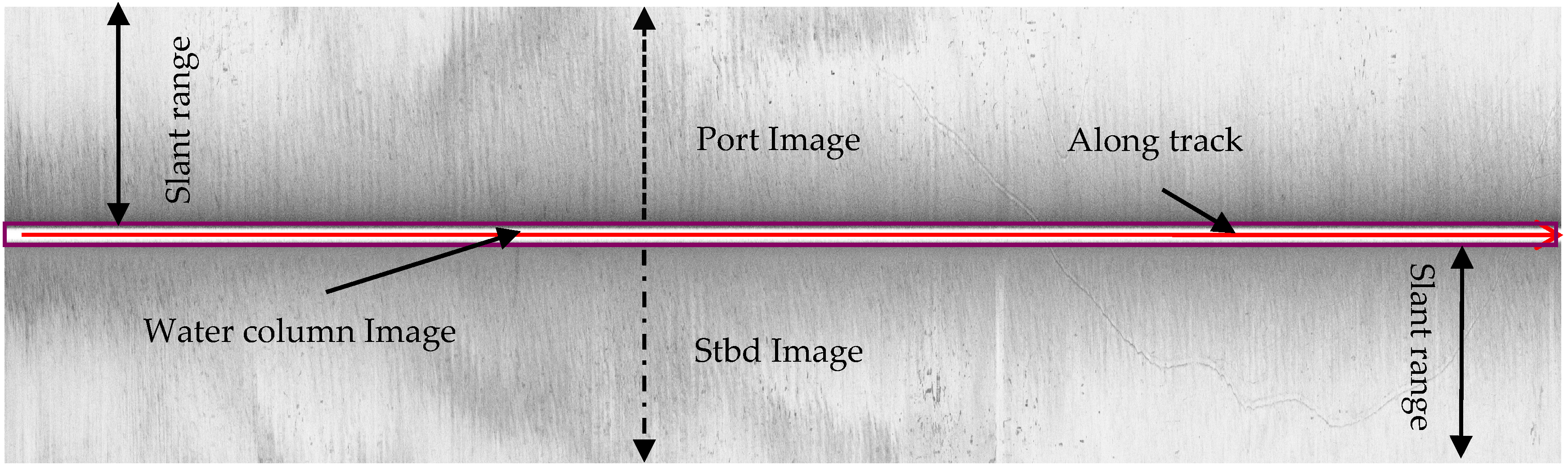
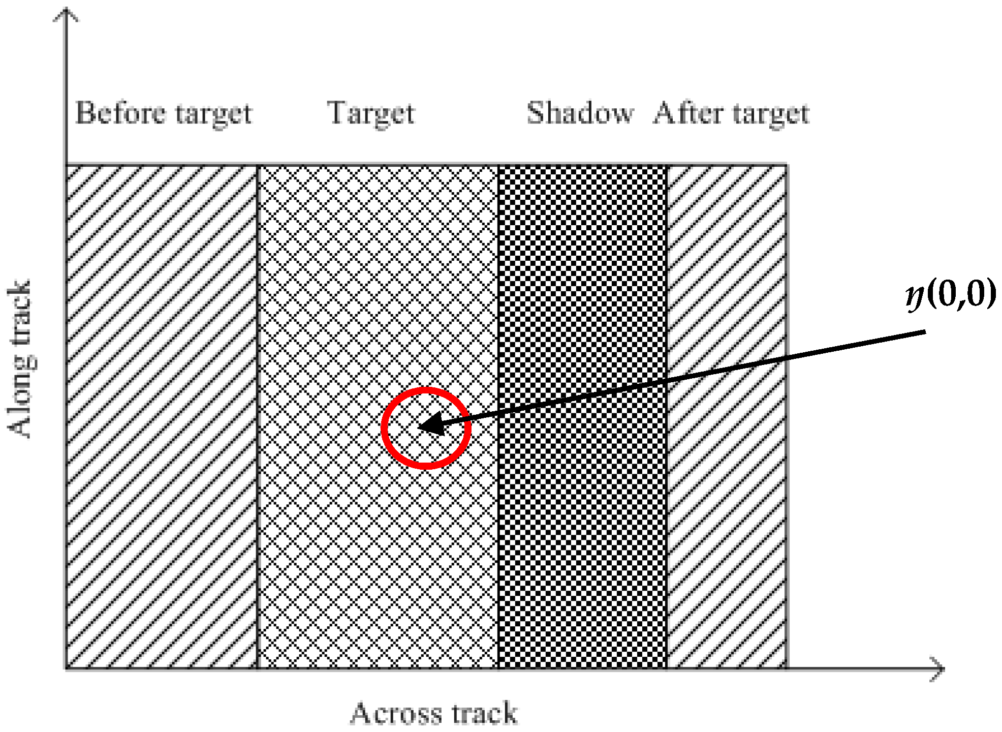
3.2.1. SSS Image Pre-Processing

According to the imaging mechanism of SSS, the SSS image was significantly influenced by the sound attenuation and the diffusion with the sound transmission distance and water properties. Additionally, as can be seen from Figure 3, the raw SSS waterfall image was seriously influenced by the radiation distortion. As such, time varying gain (TVG) and radiation distortion correction were processed by the method given in [31] for the SSS image to maintain the consistency of the gray level in the along- and across-track directions. In order to make the target areas easier to distinguish, an image enhancement was processed by:
I e ( i , j ) = min ( 4 , I r ( i , j ) / mean ( i ) ) mean ( i ) = 1 N n = N ( m ) N I r ( i , j )
where, Ie is the enhanced image and Ir is the original image; if M and N are the height and width of the image, respectively, then 1 ≤ iM, 1 ≤ jN and mean (i) is the mean value of the i-th line of the image. In order to make sure that the image enhancement was carried out separately for the port, starboard and water column images, N(i) was introduced and defined as the i-th bottom tacking result. After the above process, it can be concluded that the average gray scale value of the background region is substantially uniform, the gray scale value of the target region varies from 1 to 4, and the gray scale value of the shadow region ranges from 0 to 1. Therefore, the target areas may be detected more easily.

3.2.2. A Nonlinear Matching Model for Target Detection

With the appearance of SSS shipwreck recognition models learned from sample images, an exhaustive search can be performed where every location within the SSS image is examined so as not to miss any potential shipwreck locations. However, this type of search has several drawbacks. Searching every possible location is computationally infeasible. Consequently, an important task before shipwreck recognition is to locate those regions named as shipwreck-like areas with very different characteristics. According to the characteristics of the SSS shipwreck image, a nonlinear matching model was used to quickly detecting the shipwreck-like target areas; the model includes the shipwreck areas, the shadow areas for the shipwreck, the areas before and after the shipwreck. The schematic diagram is shown in Figure 5. The matched filter output is calculated according to:
I e ( i , j ) = k = m 1 m 2 l = n 1 n 2 g ( η ( k , l ) , I e ( i + k , j + l ) ) g ( η ( k , l ) , I e ) = { η ( k , l ) ( I e 1 ) the   shipwreck   and   its   shadow   areas η ( k , l ) | I e 1 | the   area   before   and   after   the   shipwreck h ( k , l ) = { 1 / ( T a | T 0 1 | ) the   area   before   shipwreck 1 / ( H a ( H 0 1 ) ) the   shipwreck   area 0 the   shadow   areas   of   the   shipwreck 1 / ( S a ( S 0 1 ) ) the   area   after   shipwreck
where I′e is the output of the model, Ie is the enhanced image, m2 + m1 is the length of the model in the along-track direction; n2 + n1 is the length of the model in the across-track direction and Ta, Ha and Sa indicate the value of the model in the area before shipwreck, the shipwreck area, and the area after shipwreck, if the model of the area before shipwreck is 3 × 3, then Ta = 9. Considering that the real measured SSS shipwreck data may not have a shadow area, the value in the shadow areas is given as 0; the remaining values are given by referring to Dobeck [8], T0 = 2 or 0, H0 = 1.5, S0 = 0.75; and ŋ(0,0) was defined at the center of the target area.
After the above processing, an amplitude threshold was defined. If the output of the model is larger than the threshold, the window can be determined to be a shipwreck-like region, and the target detection is completed. The threshold setting method can also be referred to Dobeck [8].

3.2.3. Diffusion Map

The shipwreck-like regions were located using the nonlinear matching model. Considering that the shipwreck may be broken, a Diffusion Map (DM) was used to locate the shipwreck region accurately. A DM is a kind of nonlinear technique for dimensionality reduction, which can embed the data in a low dimensional representation. Additionally, the diffusion distance between points is useful for estimating the local density of each pixel in the new embedding.
The diffusion distance reflects the structural information of the dataset, and this provides a measure of the differences between the dataset. The dimensionality reduction and clustering property of the diffusion map are useful for target detection, especially for SSS image which contains target, background and shadow areas. Because of the background pixels in the SSS image which would be clustered together, the shadow and target area would be distant from this cluster in the new embedding. By using the target score defined in [30,32], the target and shadow areas of SSS shipwreck image can be detected accurately.
After the above processing, the shipwreck-like regions were considered to be accurately located. The feature extraction and selection, and AdaBoost shipwreck recognition model were applied in these located regions, which can solve the problem of computationally infeasibility for exhaustive searching and improve shipwreck recognition efficiency.

4. Results

A total of 50 pieces of SSS shipwreck and 200 pieces of non-shipwreck images were selected as experimental material. These non-shipwreck images are mostly contained different types of pure sea bottom backgrounds and other targets. Most of these images were measured by various types of SSS instruments in China by ourselves, while some shipwreck or other target images were collected from other references [3,10,25,33]. These images were randomly divided in two for the training and testing experiment. In the sample data pre-processing process, the image sizes were all 128 × 128 pixels, and the images were uniformly converted to grayscale images. Therefore, in the detection process shown in Figure 4, the size of the nonlinear detection model was set as 128 × 128 pixels. The “pros and cons” evaluation criteria for the recognition model are as follows:
Assume that the number of all the test samples is P, where the shipwreck image (positive sample, true) is P1, and the non-shipwreck sample (negative sample, false) is P2. When the trained classifier is used to classify the test samples, the number of correctly classified samples is F, of which the correctly recognized shipwreck sample is F1 and the non-shipwreck sample is F2. In the binary classification problem, the trained classifier obtains two types of recognition results: Shipwreck (positive) and non-shipwreck (negative). The criteria are shown in Table 2.
In order to analyze the shipwreck recognition model in numerical method, the following three evaluation indexes can be used:
(1)
Correct recognition rate: the ratio of all correctly recognized samples to the total test samples, represented by tp:
t p = ( T P + F N ) / P = F / P
(2)
False positive rate: The ratio of the negative samples recognized as positive samples to the total negative samples, represented by fp:
f p = F P / ( F P + F N ) = ( P 2 F 2 ) / P 2
(3)
Missing detection rate: The ratio of the positive samples mistakenly recognized as negative samples to the total positive samples, represented by tn:
t n = T N / ( T P + T N ) = ( P 1 F 1 ) / P 1
In the subsequent discrimination process, it is desirable that the missing detection rate tn is as small as possible, and that the false positive rate fp is small.

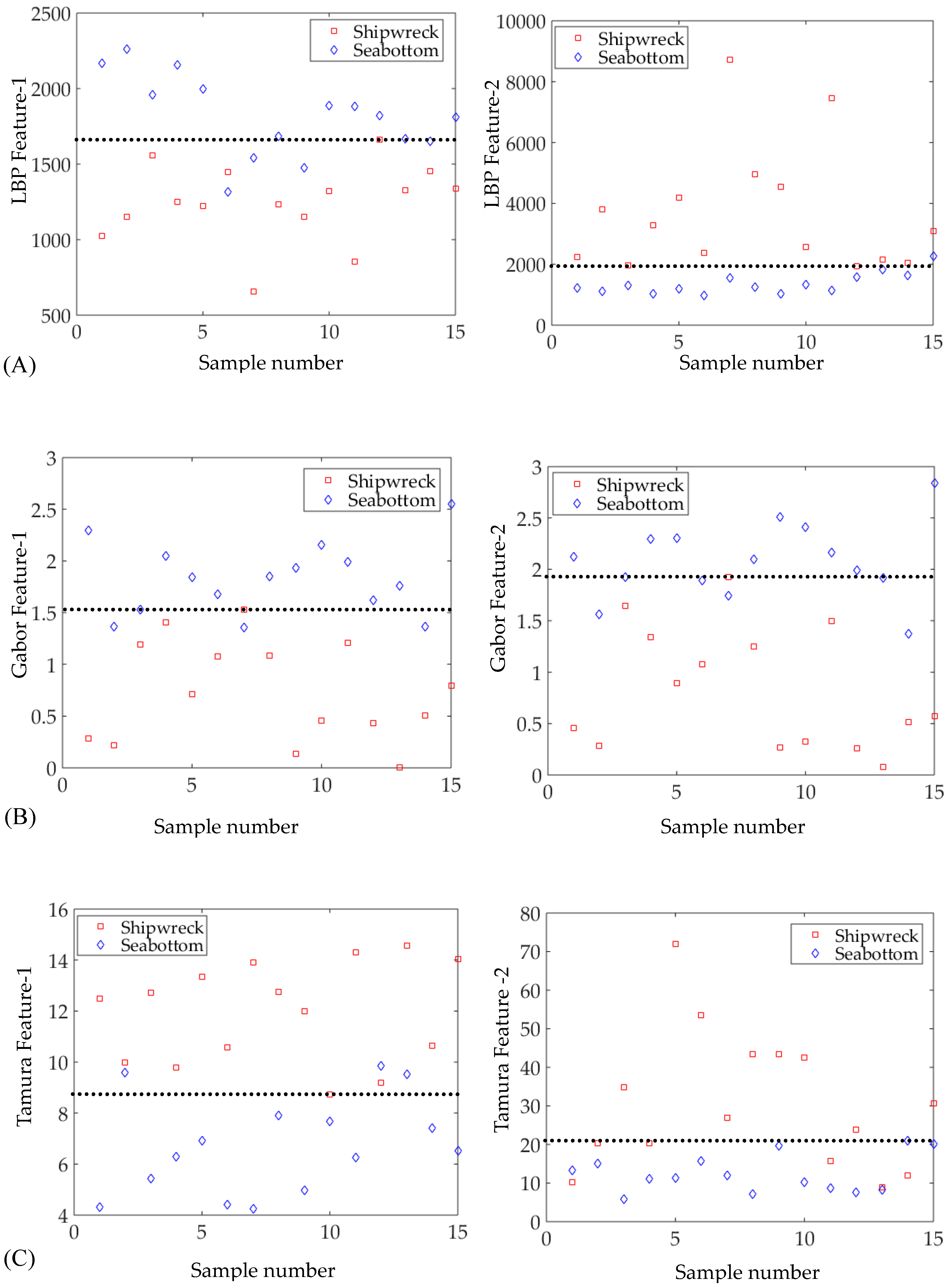
4.1. Analysis of Typical Features for Shipwreck Targets

In order to ensure the validity of the features extracted from the sample and actual measured SSS data, before the gray-scale features extraction process, the first step is to perform image enhancement, which is also a gray-scale normalization process. However, the original statistical information is expected to be obtained without image enhancement when textural features are extracted. Firstly, the numerical experiments of fractal and multifractal features extracted from SSS images of natural sea bottom background and man-made shipwreck target are carried out.
The fractal dimension D is calculated by the differential box-counting method, and the original shipwreck image and its D values are shown in Figure 6. The D was calculated in 8 × 8 neighborhoods. It can be seen that the D of the shipwreck contour is clearly different from that of the natural sea bottom background image, such that the shipwreck target can be recognized. However, it can also be seen that the D in the shadow and some background areas is smaller than the natural sea bottom background image, which may lead to the misrecognizing of the shipwreck target in SSS waterfall images.
Both Figure 1 (D was calculated by the whole image) and Figure 6 (D was calculated by the neighborhoods in one image) show the validity and defect of D for SSS shipwreck recognition.
Multifractals were calculated by the box-counting method [21]. Experiments were carried out by using SSS image of shipwreck target and natural sea bottom background of sandy slope, with uniform image sizes of 128 × 128 pixels. The numerical results of the multifractal width are shown in Figure 7. It can be seen that the multifractal width of the underwater shipwreck target was 0.5629, and that of the sea bottom image was 0.1051. The multifractal width of the SSS image of the man-made shipwreck target is larger than the natural sea bottom background image. Figure 2 and Figure 7 both demonstrate that multifractals’ width can be used to recognize the shipwreck target from SSS sea bottom image.
The above experiments show that the fractal and multifractal can distinguish man-made shipwreck target from natural sea bottom background images, and verify the theory introduced in Section 2. Next, independent features were extracted to construct a shipwreck target recognition model by different recognition algorithms. The modeling and testing data were randomly divided in two. The recognition results of the test data are shown in Table 3 and Table 4.
The commonly used gray features such as mean gray level, and comprehensive gray (CGRAY) features which combined mean gray level, mean square error, entropy and energy were also used for constructing the recognition model. The recognition results of the test data are shown in Table 5 and Table 6.
The abovementioned experiments show that a single typical feature can achieve a higher correct recognition rate than the commonly used gray features. Other evaluation indexes have more consistency, however the tp and fn indexes both still have large values. The complexity and particularity of the underwater acoustic environment also determines that no reliable single typical feature is available to construct a strong robust recognition model. In the recognition process of the shipwreck target, the missing detection rate is expected to reach zero, and the smaller the false positive rate the better. Therefore, typical and other commonly used features are combined for the next experiment, and all the evaluation indexes are compared with each other. Then, the best recognition model construction algorithm is given in the following experiment.

4.2. The Optimal Recognition Model Construction Algorithm

The commonly used features, Gray Level Co-occurrence Matrix (GLCM) and CGRAY, were combined, and then combined with the typical features to construct the shipwreck recognition model based on Gentle AdaBoost, kNN, RF and SVM, respectively. The recognition results of the test data are shown in Table 7 and Table 8.
The abovementioned experiments show that the combination of features does not obviously improve the correct recognition rate compared to that achieved when only using the typical features. However, by combining typical features with commonly used features, the capability of distinguishing shipwreck target from sea bottom images can be improved. As a result, this can reduce the missed detection rate and false positive rate. Gentle AdaBoost can not only improve the correct recognition rate, but also ensure a steady decrease of missed detection rate and false positive rate, which corresponds to the theoretical advantages mentioned in Section 3. When SVM, kNN and RF are used for constructing the recognition model, it could obtain a high correct recognition rate, however there are some drawbacks in the numerical values of the false positive rate or the missed detection rate. This is due to the influences of complex marine environment, the insufficient number of sample images, and the fact that the images were obtained from different instruments in different sea bottom background, and were affected by various noises, meaning that SVM, kNN and RF cannot work well. By analyzing the characteristics of each recognition algorithm and the experimental results, the Gentle AdaBoost algorithm was finally selected to construct the shipwreck target recognition model.

4.3. Shipwreck Target Recognition Model Construction

By combining other features extraction methods mentioned in the introduction and other literatures, considering the visual feature description of the image, the contrast, roughness and orientation for the Tamura texture feature were extracted to represent the gray features. The ring feature which characterizes roughness, and the wedge feature which characterizes direction based on the Fourier transformation, were extracted to further characterize the shipwreck texture. Considering the detailed description of the shipwreck texture in local space and frequency domain information, Gabor texture features were extracted to further enrich the texture representation of the shipwreck target. Considering that the SSS waterfall image target recognition requires multi-scale processing of the image, the local binary pattern (LBP) features are extracted to characterize multi-scale features; it is an operator used to describe the local features of SSS images, and LBP features have significant advantages such as gray and rotation invariance [34].
Some of the features mentioned above are calculated using the same images as used in Figure 1. The results are shown in Figure 8. These LBP, Gabor and Tamura features are all feature sets and have high dimensions; the feature values are only shown in several dimensions selected from the feature set. It can be seen from Figure 8 that all of these features have the ability to recognize shipwreck targets from natural sea bottom SSS image. However, the recognition performance is not as good as the typical features; more negative samples can be misrecognized as shipwreck targets through using any single texture feature value as marked by the black dotted line in Figure 8.
The above features were all combined as a comprehensive feature, whose dimension reached 427, and were used to construct the shipwreck recognition model. Based on the comprehensive feature, PCA and ICA optimized features respectively, Gentle AdaBoost was used to construct the shipwreck recognition model. The statistical results of the test data are shown in Table 9.
As shown in Table 9, the correct recognition rate of shipwreck image is very low based on the dimensionality reduction features obtained by PCA, and the missed detection rate is 1, indicating that none of the shipwrecks were recognized. This verifies that under the influence of complex marine environmental noise, and taking the images acquired by different instruments as samples, the extracted features may not necessarily satisfy a Gaussian distribution, and the target areas may not necessarily dominate the information. Therefore, a simple linear transformation cannot effectively achieve the correct extraction of the main optimal features. After the preferred features are extracted by ICA, the correct recognition rate reached 97.44% and the missed detection rate reached 0, which demonstrates that the main optimal feature components were effectively extracted. Therefore, based on the preferred features extracted by the ICA dimensionality reduction algorithm, the use of Gentle AdaBoost to construct a shipwreck recognition model is effective and feasible.

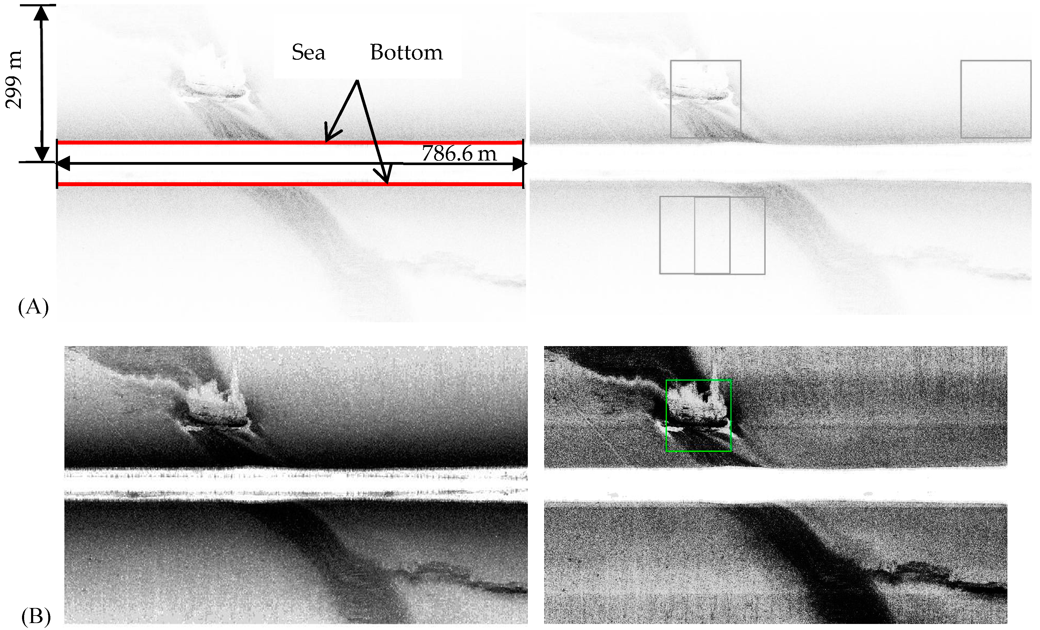
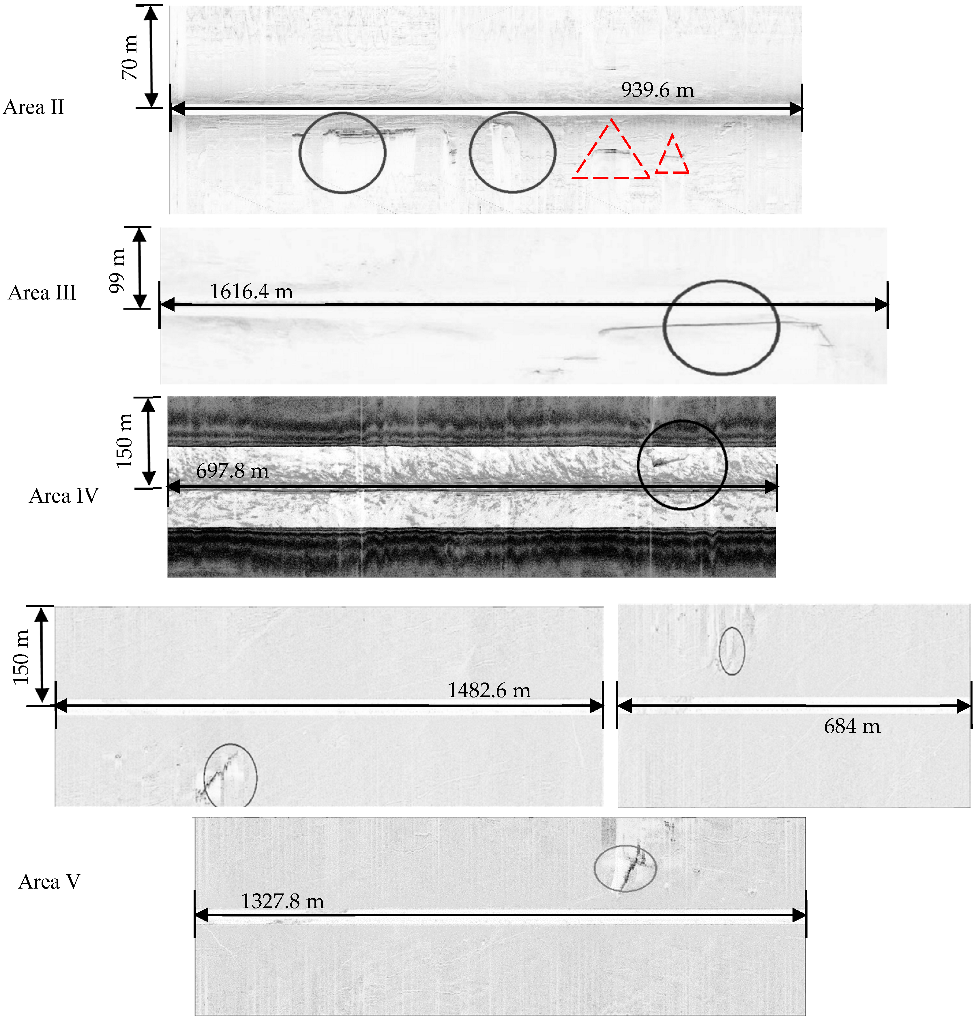
4.4. Shipwreck Target Recognition in Actual Measured SSS Waterfall Images

In order to verify the correctness of the shipwreck recognition model and process, some experiments were carried out using the actual measured SSS strip data. These experiments’ areas, instruments type, and the slant range of the strip, are shown in Table 10. The resolution of all of the images was set as 0.6 m.
First, taking the SSS image of area I as an example, and the original SSS waterfall image is used for shipwreck recognition. The SSS image and the shipwreck recognition results are shown in Figure 9A. Due to the serious radiation distortion of the image, there are obvious highlight areas in the image besides the sea bottom line. When the target was detected, 13 false targets in these areas were detected as true targets, so the subsequent recognition process was inefficient and cannot achieve accurate shipwreck target recognition, and four targets were misrecognized as shipwrecks. Subsequently, the target recognition was performed based on the SSS waterfall image corrected by radiation distortion, which was corrected by the method introduced in [31], and can ensure that the differences between the target and its’ shadow areas still exist. Four targets were detected and the shipwreck was correctly recognized after the model was identified. The radiation-distortion-corrected image and the shipwreck target recognition results are shown in Figure 9B. The experiment demonstrates that the given recognition process and model can achieve the accurate recognition of shipwreck targets in real measured SSS waterfall images.
The shipwreck recognition process was also performed in the other surveying areas. The final recognition results are shown in Figure 10. It can be seen that the given shipwreck recognition process can better recognize the shipwreck targets measured by different instruments in different sea areas; this result proves the feasibility of the process, and the Adaboost shipwreck recognition model has strong robustness and applicability. By analyzing the shipwreck target recognition results in each area shown in Figure 10, it can be seen that the shipwreck targets were well recognized in areas II, IV and V. The shipwreck targets in area II had been broken, and the recognition model recognized the main parts of the shipwreck targets. In area IV, the shipwreck target was effectively recognized by the recognition model, despite the fact that the shipwreck is located in the water column image, and the image is significantly polluted by marine noise, making it difficult to determine the type of target by visual interpretation. As can be seen in Figure 10, the shape of the shipwreck targets in all areas were not obvious, and the shipwreck target can be recognized accurately when the shape parameter cannot be obtained. In all of the above areas, the existence of a shipwreck had been confirmed by other means such as magnetic survey and human diving operations.
In area III, the target is recognized as a shipwreck by the model even though no shipwreck occurred in the area. It is found that the acoustic echoes of other ship were returned and received by the SSS transducer during the measurement and were misrecognized as shipwrecks by the model. This misrecognition can be ruled out according to the measurement log in the surveying.
It can be concluded that the shipwreck can be recognized even if the shape parameter is not available. First, we were able to extract the gray-level features, the texture features of GLCM, fractal dimension, multifractal width, Tamura, LBP, Gabor, ring and wedge texture features based on Fourier transform, etc. Then, the feature dimension reduction as an optimal feature selection process was realized by ICA. Finally, an underwater shipwreck recognition model was constructed using Gentle AdaBoost. Based on the given recognition process, the shipwreck was able to be effectively and accurately recognized. In the implementation process, it is suggested that the survey still needs to strictly follow the operational requirements and take into account the actual operating environment, to ensure that high-quality SSS images can be obtained and accurate shipwreck target recognition can be realized.

5. Discussion

These experiments verify the correctness and effectiveness of the shipwreck recognition progress used for SSS waterfall images. However, there are also some problems that will influence the accuracy and effectiveness of the shipwreck recognition.

5.1. The Effect of Nonlinear Matching Model used for Quick Object Detection

It can be seen from the areas marked by the red triangle shown in Figure 10, area II, that the two shipwreck-like broken areas were not recognized in the SSS waterfall image. In the experiment, this was caused by the missing detection during the nonlinear matching model process used for the target detection step. The shipwreck recognition was not applied in these regions. The model given in the process could solve the problem of time-consuming of exhaustive searches methods, although it reduced the shipwreck correct recognition rate.
The size of the model was set at a constant value of 128 × 128 pixels, and the model was implemented in a moving window without any overlapping during the experiment. If the target is larger than the model, the shipwreck-like region can be located; otherwise it fails. As such, a stronger robust model should be studied in depth, such as one constructed with variable length, or one in a multi-scale processed SSS waterfall image, etc.
The target detection process shown in Figure 4 includes a nonlinear matching model and DM calculation, which are expected to achieve fast and accurate location of shipwreck-like target areas. Nevertheless, this can be replaced by other effective methods, such as the methods of selective search and edge-box, which have been shown to have good application to other images collected by cameras and remote sensing satellites [35,36].

5.2. The Features and Shipwreck Recognition Model (AdaBoost) Used in the Current Process

Although the shipwreck target in SSS waterfall image could be recognized by the current process, much more work should be carried out, such as feature extraction and selection, which is time consuming and in which the quality of features seriously affects the shipwreck correct recognition rate. These shipwreck features may not be suitable for other targets, and an effective feature set for more targets is difficult to obtain. The problem influenced the accuracy and efficiency of the process. Additionally, the AdaBoost algorithm used in the experiment has the drawback of being time consuming at the model training step. Only 250 samples were used in the current experiment, just half of which were selected for the training model, which removed the drawback of excessive time consumption. However, for large datasets, this is an issue that must be addressed.
Recently, deep learning methods based on neural networks have dominated the fields of speech recognition and vision-based pattern recognition [37]. The method for constructing an underwater man-made target recognition model based on convolutional neural network (CNN) requires further study. One of the difficulties and priorities for introducing CNN in underwater target recognition is that CNN requires a huge amount of annotated data for training, while the indicator samples are difficult to acquire, especially for SSS images obtained in complex marine environment.

6. Conclusions

In this study, the Gentle AdaBoost recognition model of a side-scan sonar (SSS) shipwreck target was studied, and a shipwreck recognition process was presented for the automatic and accurate recognition of the shipwreck target in a SSS waterfall image. Firstly, the feature extraction methods suitable for shipwreck targets were studied and analyzed, and the optimal feature selection method was given based on Independent Component Analysis (ICA). Secondly, some widely used recognition algorithms were compared and analyzed, and Gentle AdaBoost was considered as a useful algorithm for underwater SSS image. A Gentle AdaBoost-based SSS shipwreck target recognition model was constructed based on the preferred features. Finally, the flow chart of shipwreck target recognition for SSS waterfall images was given. Experiments demonstrate the correctness of the shipwreck target recognition model and process. The given shipwreck target recognition process has some scalability: The recognition of other underwater special targets in SSS image, and mine-like objects, can be performed by only modifying some textural features or adding the shape feature.

Author Contributions

Conceptualization, X.W. and B.Z.; Methodology, X.W.; Software, X.W. and Y.Y.; Validation, X.W. and B.Z.; Formal Analysis, X.W.; Resources, X.W., B.Z. and Z.C.; Writing-Original Draft Preparation, X.W., B.Z. and Z.C.; Writing-Review & Editing, X.W., Y.Y., J.S. and B.Z.; Project Administration, X.W., B.Z.; Funding Acquisition, B.Z., Z.C. and X.W.

Funding

This research was supported by the National Natural Science Foundation of China (41806117), the Youth Science Foundation of Huaihai Institute of Technology (Z2017013), and the NanJing Research Institute of Surveying, Mapping & Geotechnical Investigation, Co. Ltd. (2018RD03).

Conflicts of Interest

The authors declare no conflict of interest.

References

  1. Healy, C.A.; Schultz, J.J.; Parker, K.; Lowers, B. Detecting Submerged Bodies: Controlled Research Using Side-Scan Sonar to Detect Submerged Proxy Cadaver. J. Forensic Sci. 2015, 60, 743–752. [Google Scholar] [CrossRef] [PubMed]
  2. Kumagai, H.; Tsukioka, S.; Yamamoto, H.; Tsuji, T.; Shitashima, K.; Asada, M.; Yamamoto, F.; Kinoshita, M. Hydrothermal plumes imaged by high-resolution side-scan sonar on a cruising AUV, Urashima. Geochem. Geophys. Geosyst. 2010, 11, 1–8. [Google Scholar] [CrossRef]
  3. Davy, C.M.; Fenton, M.B. Technical note: Side-scan sonar enables rapid detection of aquatic reptiles in turbid lotic systems. Eur. J. Wildl. Res. 2013, 59, 123–127. [Google Scholar] [CrossRef]
  4. Bryant, R. Side Scan Sonar for Hydrography-An Evaluation by the Canadian Hydrographic Service. Int. Hydrogr. Rev. 2015, 52, 243–249. [Google Scholar]
  5. Flowers, H.J.; Hightower, J.E. A novel approach to surveying sturgeon using side-scan sonar and occupancy modeling. Mar. Coast. Fish. 2013, 5, 211–223. [Google Scholar] [CrossRef]
  6. Nakamura, K.; Toki, T.; Mochizuki, N.; Asada, M.; Ishibashi, J.I.; Nogi, Y.; Yoshikawa, S.; Miyazaki, J.I.; Okino, K. Discovery of a new hydrothermal vent based on an underwater, high-resolution geophysical survey. Deep Sea Res. Part I: Oceanogr. Res. Pap. 2013, 74, 1–10. [Google Scholar] [CrossRef]
  7. Ramirez, T.M. Triton-Sidescan Processing Guide—Software Version 7.6; Triton Imaging Inc.: Capitola, CA, USA, 2014; pp. 6–7. [Google Scholar]
  8. Dobeck, G.J.; Hyland, J.C. Automated detection and classification of sea mines in sonar imagery. In Detection and Remediation Technologies for Mines and Minelike Targets II; International Society for Optics and Photonics: Bellingham, WA, USA, 1997; pp. 90–110. [Google Scholar]
  9. Dobeck, G.J. Algorithm fusion for the detection and classification of sea mines in the very shallow water region using side-scan sonar imagery. In Detection and Remediation Technologies for Mines and Minelike Targets V; International Society for Optics and Photonics: Bellingham, WA, USA, 2000; pp. 348–361. [Google Scholar]
  10. Reed, S.; Petillot, Y.; Bell, J. An automatic approach to the detection and extraction of mine features in sidescan sonar. IEEE J. Ocean. Eng. 2003, 28, 90–105. [Google Scholar] [CrossRef] [Green Version]
  11. Langner, F.; Knauer, C.; Jans, W.; Ebert, A. Side Scan Sonar Image Resolution and Automatic Object Detection, Classification and Identification. In Proceedings of the OCEANS 2009—Europe Conference, Bremen, Germany, 11–14 May 2009. [Google Scholar]
  12. Isaacs, J.C. Sonar automatic target recognition for underwater UXO remediation. In Proceedings of the 2015 IEEE Conference on Computer Vision and Pattern Recognition Workshops (CVPRW), Boston, MA, USA, 7–12 June 2015; pp. 134–140. [Google Scholar]
  13. Guo, H.; Tian, T. A Recognizing Method Based on Fuzzy Clustering on the Sonar Image of a Small Target on the Sea Bed. J. Chin. Comput. Syst. 2002, 23, 139–141. [Google Scholar]
  14. Wang, B. Research on Sonar Image Processing and Target Recognition. Master’s Thesis, Northwest Normal University, Lanzhou, China, 2005. [Google Scholar]
  15. Yang, F.; Du, Z.; Wu, Z. Object Recognizing on Sonar Image Based on Histogram and Geometric Feature. Mar. Sci. Bull. 2006, 25, 64–69. [Google Scholar]
  16. Ma, M. Study on Under Water Target Recognition Technique. Master’s Thesis, Harbin Engineering University, Harbin, China, 2007. [Google Scholar]
  17. Tang, C. Research on Multi-resolution Analysis and Recognition of Underwater Targets Acoustic Image. Ph.D. Thesis, Harbin Engineering University, Harbin, China, 2009. [Google Scholar]
  18. Nayak, S.R.; Mishra, J.; Palai, G. A modified approach to estimate fractal dimension of gray scale images. Optik 2018, 161, 136–145. [Google Scholar] [CrossRef]
  19. Nelson, S.R.; Tuovila, S.M. Fractal Features Used with Nearest Neighbor Clustering for Identifying Clutter in Sonar Images. U.S. Patent US 6,052,485, 18 April 2000. [Google Scholar]
  20. Tin, H.W.; Leu, S.W.; Wen, C.C.; Chang, S.H. An efficient side scan sonar image denoising method based on a new roughness entropy fractal dimension. In Proceedings of the 2013 IEEE International Underwater Technology Symposium (UT), Tokyo, Japan, 5–8 March 2013; pp. 1–5. [Google Scholar]
  21. Islam, A.; Reza, S.M.; Iftekharuddin, K.M. Multifractal texture estimation for detection and segmentation of brain tumors. IEEE Trans. Biomed. Eng. 2013, 60, 3204–3215. [Google Scholar] [CrossRef] [PubMed]
  22. Lopes, R.; Betrouni, N. Fractal and multifractal analysis: A review. Med. Image Anal. 2009, 13, 634–649. [Google Scholar] [CrossRef] [PubMed]
  23. Hasan, M.K.; Sakib, N.; Field, J.; Love, R.R.; Ahamed, S.I. Bild (big image in less dimension): A novel technique for image feature selection to apply partial least square algorithm. In Proceedings of the 2017 IEEE Great Lakes Biomedical Conference (GLBC), Milwaukee, WI, USA, 6–7 April 2017; pp. 1–10. [Google Scholar]
  24. Chizi, B.; Maimon, O. Dimension Reduction and Feature Selection. J. Appl. Entomol. 2016, 140, 444–452. [Google Scholar]
  25. Fakiris, E.; Papatheodorou, G.; Geraga, M.; Ferentinos, G. An Automatic Target Detection Algorithm for Swath Sonar Backscatter Imagery, Using Image Texture and Independent Component Analysis. Remote Sens. 2016, 8, 373. [Google Scholar] [CrossRef]
  26. Guo, G.; Wang, H.; Bell, D.; Bi, Y.; Greer, K. KNN Model-Based Approach in Classification. In Otm Confederated International Conferences on the Move to Meaningful Internet Systems; Springer: Berlin/Heidelberg, Germany, 2003; pp. 986–996. [Google Scholar]
  27. Cutler, D.R.; Edwards, T.C., Jr.; Beard, K.H.; Cutler, A.; Hess, K.T.; Gibson, J.; Lawler, J.J. Random Forests for Classification in Ecology. Ecology 2007, 88, 2783–2792. [Google Scholar] [CrossRef] [PubMed]
  28. Matic-Cuka, B.; Kezunovic, M. Islanding Detection for Inverter-Based Distributed Generation Using Support Vector Machine Method. IEEE Trans. Smart Grid 2017, 5, 2676–2686. [Google Scholar] [CrossRef]
  29. Bi, J.; Chen, J.; Yang, S.; Li, C.; Wang, J.; Zhang, B. A Face Detection Method Based on LAB and Adaboost. In Proceedings of the 2016 International Conference on Virtual Reality and Visualization (ICVRV), Hangzhou, China, 24–26 September 2017; pp. 175–178. [Google Scholar]
  30. Wang, X.; Zhao, J.; Zhu, B.; Jiang, T.; Qin, T. A Side Scan Sonar Image Target Detection Algorithm Based on a Neutrosophic Set and Diffusion Maps. Remote Sens. 2018, 10, 295. [Google Scholar] [CrossRef]
  31. Zhao, J.; Yan, J.; Zhang, H.; Meng, J. A New Radiometric Correction Method for Side-Scan Sonar Images in Consideration of Seabed Sediment Variation. Remote Sens. 2017, 9, 575. [Google Scholar] [CrossRef]
  32. Mishne, G.; Cohen, I. Multiscale anomaly detection using diffusion maps and saliency score. In Proceedings of the IEEE International Conference in Acoustics, Speech and Signal Processing (ICASSP), Florence, Italy, 4–9 May 2014; pp. 2823–2827. [Google Scholar]
  33. Zhao, J.; Wang, X.; Zhang, H.; Hu, J.; Jian, X. Side scan sonar image segmentation based on neutrosophic set and quantum-behaved particle swarm optimization algorithm. Mar. Geophys. Res. 2016, 37, 229–241. [Google Scholar] [CrossRef]
  34. Singh, G.; Chhabra, I. Effective and Fast Face Recognition System Using Complementary OC-LBP and HOG Feature Descriptors with SVM Classifier. J. Inf. Technol. Res. 2018, 11, 91–110. [Google Scholar] [CrossRef]
  35. Uijlings, J.R.; Van De Sande, K.E.; Gevers, T.; Smeulders, A.W. Selective Search for Object Recognition. Int. J. Comput. Vis. 2013, 104, 154–171. [Google Scholar] [CrossRef] [Green Version]
  36. Zhao, Z.B.; Zhang, L.; Qi, Y.C.; Shi, Y.Y. A Generation Method of Insulator Region Proposals Based on Edge Boxes. Optoelectron. Lett. 2017, 13, 466–470. [Google Scholar] [CrossRef]
  37. Chen, F.C.; Jahanshahi, M.R. NB-CNN: Deep Learning-Based Crack Detection Using Convolutional Neural Network and Naïve Bayes Data Fusion. IEEE Trans. Ind. Electron. 2018, 65, 4392–4400. [Google Scholar] [CrossRef]
Figure 1. The value of fractal dimension (D) calculated by Side Scan Sonar (SSS) images of shipwreck and sea bottom. The black dotted line represents the feature distinguishing value. The elliptical labeling area are the samples difficult to be recognized.
Remotesensing 11 00243 g001
Figure 2. The value of multifractal width calculated by SSS images of shipwreck and sea bottom.
Remotesensing 11 00243 g002
Figure 3. SSS waterfall image, it was measured in the South China Sea by Edgetech 4200 MP system.
Remotesensing 11 00243 g003
Figure 4. Shipwreck target recognition process for SSS waterfall image [8,30,31,32].
Remotesensing 11 00243 g004
Figure 5. Schematic diagram of the matching model.
Remotesensing 11 00243 g005
Figure 6. Shipwreck image and its fractal dimension (D), the raw SSS image is referenced from [33]. The red ellipse marked area demonstrate the shipwreck contour.
Remotesensing 11 00243 g006
Figure 7. Comparison of the multifractal width of shipwreck and sea bottom image, the sea bottom image is intercepted from Figure 3.
Remotesensing 11 00243 g007
Figure 8. The value of other texture features calculated by SSS images of shipwreck and sea bottom. The black dotted line represents the feature distinguishing value. (A) shows the first two dimensions of local binary pattern (LBP) features, (B) shows the first two dimensions of Gabor features, (C) shows the first two dimensions of Tamura features.
Remotesensing 11 00243 g008
Figure 9. The shipwreck target recognition result in area I. (A) The raw SSS image is used for the experiment; (B) The radiation distortion corrected image is used for the experiment.
Remotesensing 11 00243 g009
Figure 10. The shipwreck target recognition results in other surveying areas.
Remotesensing 11 00243 g010
Table 1. The flowchart of k-Nearest Neighbors (kNN) algorithm.
kNN
1. Calculate the distance between the current point and the point in the known category data set;
2. Sorting these points according to Lp distance, if p = 2, this is Euclidean distance;
3. Select the smallest k points from the current point;
4. Determine the frequency of occurrence of the previous k points;
5. Return to the category with the highest frequency of occurrences at the previous k points as the forecast classification result.
Table 2. Discriminant criteria for dichotomous problems.
TrueFalse
PositiveTrue Positve (TP)False Positive (FP)
NegativeTrue Negative (TN)False Negative (FN)
Table 3. Experimental results of constructing different recognition models based on D.
Feature − DCorrect Recognition Rate (%)False Positive Rate (%)Missed Detection Rate (%)
Gentle AdaBoost92.316.256.67
kNN92.316.256.67
SVM63.896.250
RF92.316.256.67
Table 4. Experimental results of constructing different recognition models based on multifractal width.
Feature − Multifractal WidthCorrect Recognition Rate (%)False Positive Rate (%)Missed Detection Rate (%)
Gentle AdaBoost94.873.136.67
kNN94.873.134.29
SVM97.4404.29
RF94.873.134.29
Table 5. Experimental results of constructing different recognition models based on mean gray level.
Feature − Mean Gray LevelCorrect Recognition Rate (%)False Positive Rate (%)Missed Detection Rate (%)
Gentle AdaBoost31.2591.1814.29
kNN2579.4164.29
SVM35.4276.4735.71
RF2579.4164.29
Table 6. Experimental results of constructing different recognition models based on comprehensive gray (CGRAY).
Feature − CGRAYCorrect Recognition Rate (%)False Positive Rate (%)Missed Detection Rate (%)
Gentle AdaBoost58.3350.0021.43
kNN2579.4164.29
SVM29.171000
RF64.5847.067.14
Table 7. Experimental results of constructing different recognition models based on Gray Level Co-occurrence Matrix (GLCM) + CGRAY features.
Features − GLCM + CGRAYCorrect Recognition Rate (%)False Positive Rate (%)Missed Detection Rate (%)
Gentle AdaBoost92.30773.1328.57
kNN92.30779.380
SVM94.87183.1314.29
RF92.30773.1328.57
Table 8. Experimental results of constructing different recognition models based on GLCM + CGRAY + multifractal width features.
Features − GLCM + CGRAY + Multifractal WidthCorrect Recognition Rate (%)False Positive Rate (%)Missed Detection Rate (%)
Gentle AdaBoost94.871806.7
kNN92.30779.380
SVM94.4539014.29
RF94.8718028.57
Table 9. Experimental results of constructing shipwreck recognition model by Gentle AdaBoost based on comprehensive feature, preferred feature extracted by Principal Component Analysis (PCA) and Independent Component Analysis (ICA) respectively.
Correct Recognition Rate (%)False Positive Rate (%)Missed Detection Rate (%)
Comprehensive Feature92.313.1328.57
PCA Feature extraction82.050100
ICA Feature extraction97.443.130
Table 10. The surveying areas and SSS instruments used for the experiments.
Instruments’ TypeSlant Range (m)Experiment AreasResolution (m)
IBenthos SIS 1624299East China Sea0.6
IIEdgeTech 420070Shenzhen Bay0.6
IIIBenthos SIS 162499South of Bohai0.6
IVEdgeTech 4200150North of Bohai0.6
VEdgeTech 4200150West of Bohai0.6

