Deep Convolutional Capsule Network for Hyperspectral Image Spectral and Spectral-Spatial Classification

Abstract

Capsule networks can be considered to be the next era of deep learning and have recently shown their advantages in supervised classification. Instead of using scalar values to represent features, the capsule networks use vectors to represent features, which enriches the feature presentation capability. This paper introduces a deep capsule network for hyperspectral image (HSI) classification to improve the performance of the conventional convolutional neural networks (CNNs). Furthermore, a modification of the capsule network named Conv-Capsule is proposed. Instead of using full connections, local connections and shared transform matrices, which are the core ideas of CNNs, are used in the Conv-Capsule network architecture. In Conv-Capsule, the number of trainable parameters is reduced compared to the original capsule, which potentially mitigates the overfitting issue when the number of available training samples is limited. Specifically, we propose two schemes: (1) A 1D deep capsule network is designed for spectral classification, as a combination of principal component analysis, CNN, and the Conv-Capsule network, and (2) a 3D deep capsule network is designed for spectral-spatial classification, as a combination of extended multi-attribute profiles, CNN, and the Conv-Capsule network. The proposed classifiers are tested on three widely-used hyperspectral data sets. The obtained results reveal that the proposed models provide competitive results compared to the state-of-the-art methods, including kernel support vector machines, CNNs, and recurrent neural network.

1. Introduction

The task of classification, when it relates to hyperspectral images (HSIs), generally refers to assigning a label to each pixel vector in the scene [1]. HSI classification is a crucial step for a plethora of applications including urban development [2,3,4], land change monitoring [5,6,7], scene interpretation [8,9], resource management [10,11], and so on. Due to the fundamental importance of this step in various applications, classification of HSI is one of the hottest topics in the remote sensing community. However, the classification of HSI is still challenging due to several factors such as high dimensionality, a limited number of training samples, and complex imaging situations [1].

During the last few decades, a huge number of methods have been proposed for HSI classification [12,13,14]. Due to the availability of abundant spectral information in HSIs, lots of spectral classifiers have been proposed for HSI classification including k-nearest-neighbors, maximum likelihood, neural network, logistic regression, and support vector machines (SVMs) [1,15,16].

Hyperspectral sensors provide rich spatial information as well, and the spatial resolution is becoming finer and finer along with the development of sensor technologies. With the help of spatial information, classification performance can be greatly improved [17]. Among the spectral-spatial classification techniques, the generation of a morphological profile is a widely-used approach, which is usually followed by either an SVM or a random forest classifier to obtain the final classification result [18,19,20,21]. As the extension of SVM, multiple kernel learning is another main stream of spectral-spatial HSI classification, which has a powerful capability to handle the heterogeneous features obtained by spectral-spatial hyperspectral images [22].

Due to the complex atmospheric conditions, scattering from neighboring objects, intra-class variability, and varying sunlight intensity, it is very important to extract invariant and robust features from HSIs for accurate classification. Deep learning uses hierarchical models to extract invariant and discriminate features from HSIs in an effective manner and usually leads to accurate classification. During the past few years, many deep learning methods have been proposed for HSI classification. Deep learning includes a broader family of models, including the stacked auto-encoder, the deep belief network, the deep convolutional neural network (CNN), and the deep recurrent neural network. All of the aforementioned deep models have been used for HSI classification [23,24].

The stacked auto-encoder was the first deep model to be investigated for HSI feature extraction and classification [25]. In [25], two stacked auto-encoders were used to hierarchically extract spectral and spatial features. The extracted invariant and discriminant features led to a better classification performance. Furthermore, recently, the deep belief network was introduced for HSI feature extraction and classification [26,27].

Because of the unique and useful model architectures of CNNs (e.g., local connections and shared weights), such networks usually outperform other deep models in terms of classification accuracy. In [28], a well-designed CNN with five layers was proposed to extract spectral features for accurate classification. In [29], a CNN-based spectral classifier that elaborately uses pixel-pair information was proposed, and it was shown to obtain good classification performance under the condition of a limited number of training samples.

Most of the existing CNN-based HSI classification methods have been generalized to consider both spectral and spatial information in a single classification framework. The first spectral-spatial classifier based on CNN was introduced in [30], which was a combination of principal component analysis (PCA), deep CNN, and logistic regression. Due to the fact that the inputs of deep learning models are usually 3D data, it is reasonable to design 3D CNNs for HSI spectral-spatial classification [31,32]. Furthermore, CNN can be combined with other powerful techniques to improve the classification performance. In [33], CNN was combined with sparse representation to refine the learnt features. CNNs can be connected with other spatial feature extraction methods, such as morphological profiles and Gabor filtering, to further improve the classification performance [34,35].

The pixel vector of HSIs can be inherently considered to be sequential. Recurrent neural networks have the capability of characterizing sequential data. Therefore, in [27], a deep recurrent neural network that can analyze hyperspectral pixel vectors as sequential data and then determine information categories via network reasoning was proposed.

Although deep learning models have shown their capabilities for HSI classification, some disadvantages exist which downgrade the performance of such techniques. In general, deep models require a huge number of training samples to reliably train a large number of parameters in their networks. On the other hand, having insufficient training samples is a frequent problem in remotely sensed image classification. In 2017, Sabour et al. proposed a new idea based on capsules, which showed its advantages in coping with a limited number of training samples [36]. Furthermore, traditional CNNs usually use a pooling layer to obtain invariant features from the input data, but the pooling operation loses the precise positional relationship of features. In hyperspectral remote sensing, abundant spectral information and the positional relationship in a pixel vector are the crucial factors for accurate spectral classification. Therefore, it is important to maintain the precise positional relationship in the feature extraction stage. In addition, when it comes to extracting spectral-spatial features from HSI, it is also important to hold the positional relationship of spectral-spatial features. Moreover, most of the existing deep methods use a scalar value to represent the intensity of a feature. In contrast, capsule networks use vectors to represent features. The usage of vectors enriches the feature representation and is a huge progress and a much more promising method for feature learning than scalar representation [36,37]. These properties of the capsule network perfectly align with the goals of this study and the current demands in the hyperspectral community.

Deep learning-based methods, including deep capsule networks, have a powerful feature extraction capability when the number of training samples is sufficient. Unfortunately, the availability of only a limited number of training samples is a common bottleneck in HSI classification. Deep models are often over-trained with a limited number of training samples, which downgrades the classification accuracy on test samples. In order to mitigate the overfitting problem and lessen the feature extraction workload of deep models, the idea of a local connection-based capsule network is proposed in this study. The proposed Conv-Capsule network uses local connections and shared transform matrices to reduce the number of trainable parameters compared to the original capsule, which potentially mitigates the overfitting issue when the number of available training samples is limited.

In the current study, the idea of the capsule network is modified for HSI classification. Two deep capsule classification frameworks, 1D-Capsule and 3D-Capsule, are proposed as spectral and spectral-spatial classifiers, respectively. Furthermore, two modified capsule networks, i.e., 1D-Conv-Capsule and 3D-Conv-Capsule, are proposed to further improve the classification accuracy.

The main contributions of the paper are briefly summarized as follows.

(1)

A modification of the capsule network named Conv-Capsule is proposed. The Conv-Capsule uses local connections and shared transform matrices in the network, which reduces the number of trainable parameters and mitigates the overfitting issue in classification.

(2)

Two frameworks, called 1D-Capsule and 3D-Capsule, based on the capsule network are proposed for HSI classification.

(3)

To further improve the HSI classification performance, two frameworks, called 1D-Conv-Capsule and 3D-Conv-Capsule, are proposed.

(4)

The proposed methods are tested on three well-known hyperspectral data sets under the condition of having a limited number of training samples.

The rest of the paper is organized as follows. Section 2 presents the background of the deep learning and capsule network. Section 3 and Section 4 are dedicated to the details of the proposed deep capsule network frameworks, including spectral and spectral-spatial architectures for HSI classification. The experimental results are reported in Section 5. In Section 6, the conclusions and discussions are presented.

2. Background

2.1. Convolutional Neural Networks

In general, CNN is a special case of deep neural network, which is loosely inspired by the biological visual system [38]. Compared with other deep learning methods, there are two unique factors in the architecture of the CNN, i.e., local connections and shared weights. Since each neuron only responds to a small region known as the reception field, CNN efficiently explores the structure correlation. Furthermore, CNN uses the replicated weights and biases across the entire layer, which significantly reduces the parameters in the network. By using specific architectures like local connections and shared weights, CNN tends to provide better generalization for a wide variety of applications.

There are three main building blocks in CNNs: A convolution layer, a nonlinear transformation, and a pooling operation. By stacking several convolution layers with the nonlinear operations and several pooling layers, a deep CNN can be established [39].

A convolutional layer can be defined as follows:

$$x_j^l=f\left({{\displaystyle \sum }}_{i=1}^M{x}_i^{l-1}*k_{ij}^l+b_j^l\right),$$

(1)

$$f\left(x\right)=\max \left(0,x\right),$$

(2)

where matrix $x_i^{l-1}$ is the i-th feature map of the previous (l-1)-th layer, $x_j^l$ is the j-th feature map of the current l-th layer, and M is the number of input feature maps. $k_{ij}^l$ and $b_j^l$ are randomly initialized and set to zero. Furthermore, $f(·)$ is a nonlinear function known as the rectified linear unit (ReLU), and ∗ is the convolution operation [40].

The pooling operation offers invariance by reducing the resolution of the feature maps. The neuron in the pooling layer combines a small N × N (e.g., N = 2) patch of the convolution layer. The most common pooling operation is max pooling.

All parameters in the deep CNN model are trained using the back-propagation algorithm.

In this study, CNN is adopted as the feature extraction method, and the extracted features are fed to the deep capsule network for further processing.

2.2. Capsule Network

The capsule network is a modification of the traditional neural network, which uses a group of neurons to obtain the vector representations of a specific type of entity.

In [36], the input to a capsule $s_j$ is a weighted sum of prediction vector $u_{j|i}$ from the previous layers. $u_{j|i}$ is obtained by multiplying $u_i$ of the previous capsule by a transform matrix $W_{ij}$,

$$s_j={{\displaystyle \sum }}_i{c}_{ij}{u}_{j|i},$$

(3)

$$u_{j|i}=W_{ij}{u}_i$$

(4)

where $c_{ij}$ represents the coupling coefficients determined by a processing called dynamic routing [36].

The capsule uses the length of the output vector to obtain the probability of the entity, and then, a nonlinear function which we call squash function is used to squash the vector,

$$v_j=\frac{||s_j||{}^2}{1+||s_j||{}^2}\frac{s_j}{||s_j||},$$

(5)

where $v_j$ is the output of capsule j, which is a vector representation of the input, while the traditional neural network uses a scalar value to give the final probability of the entity. There are some advantages when we use a vector representation instead of a scalar value. The vector representation uses the length of the activity vector to obtain the probability of the entity, and the vector representation gives the orientation of the entity too. In traditional CNNs, a pooling layer is used to make the network invariant to small changes in inputs, but the effectiveness is limited [37]. CNNs are not robust to translation, rotation, and scale, which usually downgrades their classification performance. In the capsule network, the output of the capsule is a vector representation of a type of entity [36]. When changes occur on the entity, the length of the corresponding output vector of the capsule may not change greatly. Through the capsule network, we can obtain a more robust representation of the input.

2.3. Capsule Network for HSI Classification

The capsule network can be combined with the traditional neural network (e.g., CNN) to formulate a classification system for a specific task (e.g., HSI classification). In the remote sensing community, two works have already adopted the capsule networks for HSI classification. Paoletti et al. [41] and Deng et al. [42] adopted the capsule network for HSI classification and achieved good classification performance. In this context, Paoletti et al. proposed a spectral-spatial capsule network to capture high abstract-level features for HSI classification while reducing the network design complexity. The classification result in [41] demonstrates that the proposed method can extract more relevant and complete information about HSI data cubes. Deng et al. presented a modified two-layer capsule network capable of handling a limited number of training samples for HSI classification.

Previous capsule networks contained a fully-connected capsule layer, which led to lots of trainable parameters. As we all know, having lots of parameters may cause an overfitting problem with a limited number of training samples. In this study, an improved capsule network named Conv-Capsule, which uses local connections and shared transform matrices in the network, is proposed. Conv-Capsule dramatically reduces the number of trainable parameters and mitigates the overfitting issue in HSI classification. Furthermore, the previous capsule networks for HSI classification are spectral-spatial classifiers. In this study, a 1D capsule network is also proposed as a spectral classifier to enrich the classification techniques of HSI. The details of our proposed methods are explicitly explained in Section 3 and Section 4.

3. One-Dimensional Deep Capsule Network as a Spectral Classifier

3.1. One-Dimensional Convolutional Capsule

Deep learning models use multilayer neural networks to hierarchically extract the features of input data, which is the key factor for effectiveness in deep learning-based methods. The traditional capsule network does not contain multiple capsule layers. Therefore, it is necessary to build a multilayer capsule network.

The simple stacking of capsule layers can develop a deep capsule network. However, the traditional capsule layer is fully connected and contains a huge number of trainable parameters. The problem is even worse when the number of training samples is limited. Inspired by the CNN, local connections and shared transform matrices, which are the core ideas of CNN, are combined with the dynamic routing algorithm in the capsule layer, and we call it the convolutional capsule (Conv-Capsule) layer. In the Conv-Capsule layer, each capsule in the current layer only connects with capsules within its local receptive field in the last capsule layer. The transform matrices in the local connections are shared across the entire layer.

In HSI classification, spectral classification is an important research direction. To develop a 1D capsule network for HSI classification, a 1D Conv-Capsule layer needs to be utilized. Here is a description of the 1D Conv-Capsule layer which we use here to shape the spectral classifier. The input of a capsule $s_j^x$ in a 1D Conv-Capsule layer is a weighted sum of the “prediction vector” $u_{j|i}^{x+p}$ from all channels of the capsule within its receptive field in the last capsule layer. Furthermore, $u_{j|i}^{x+p}$ is obtained by multiplying $u_i^{x+p}$ from the capsule in the last layer by the corresponding transform matrix $W_{ij}^p$ which is shared across the last capsule layer. By using a squash function, the output of the capsule $v_j^x$ can be obtained from the input $s_j^x$. The equations used here are listed as follows:

$$u_{j|i}^{x+p}=W_{ij}^p{u}_i^{x+p},$$

(6)

$$s_j^x={{\displaystyle \sum }}_{i=1}^I{{\displaystyle \sum }}_{p=0}^{P-1}{c}_{ij}^p{u}_{j|i}^{x+p},$$

(7)

$$v_j^x=squash\left(s_j^x\right),$$

(8)

where I and P are the number of capsule channels in the last capsule layer and kernel size in the current 1D Conv-Capsule layer. $s_j^x$ is the input of the j-th channel capsule at position x in the current 1D Conv-Capsule layer, and $v_j^x$ is the corresponding output. $u_i^{x+p}$ is the output of the i-th channel capsule at position (x + p) in the last capsule layer. $W_{ij}^p$ is the transform matrix between $u_i^{x+p}$ and $v_j^x$. $c_{ij}^p$ represents the coupling coefficients determined by the dynamic routing algorithm. An illustration of the 1D Conv-Capsule layer is shown in Figure 1.

3.2. Dynamic Routing Algorithm in 1D Conv-Capsule layer

Between two consecutive capsule layers, we use the dynamic routing algorithm to iteratively update coupling coefficients. The details about the procedure of the dynamic routing algorithm in 1D Conv-Capsule layer are described as follows:

From the description of the 1D Conv-Capsule in the last subsection, we know that each capsule in the current 1D Conv-Capsule layer receives “prediction vectors” from the capsules within its receptive field in the last capsule layer. The weight of each “prediction vector” is represented by coupling coefficients. The coupling coefficients between capsule $u_i^{x+p}$ in the last capsule layer and all channels capsules at the same position in the 1D Conv-Capsule layer sum to 1 and can be obtained by a softmax function,

$$c_{ij}^p=\frac{exp\left(b_{ij}^p\right)}{{{\displaystyle \sum }}_k{b}_{ik}^p},$$

(9)

where $b_{ij}^p$ is initialized to 0 before the training begins and is determined by the dynamic routing algorithm.

In the dynamic routing algorithm, the coefficient $b_{ij}^p$ is iteratively refined by measuring the agreement between the “prediction vector” $u_{j|i}^{x+p}$ and $v_j^x$. If the agreement is reached to a great extent, capsule $u_i^{x+p}$ makes a good prediction for capsule $v_j^x$. Then, the coefficient $b_{ij}^p$ will be significantly increased. In our network, the agreement is quantified as the inner product between two vectors $u_{j|i}^{x+p}$ and $v_j^x$. This agreement is added to $b_{ij}^p$:

$$a_{ij}^p=u_{j|i}^{x+p}·v_j^x,$$

(10)

$$b_{ij}^p\leftarrow b_{ij}^p+a_{ij}^p,$$

(11)

The pseudo codes of the dynamic routing algorithm in the 1D Conv-Capsule layer are shown in

Table 1. Dynamic Routing Algorithm in 1D Conv-Capsule layer.

Algorithm 1. Dynamic Routing Algorithm in 1D Conv-Capsule layer

1. begin

2.   for x in spectral dimension in current capsule layer

3.    for j-th channel capsule in current capsule layer

4.     for p across kernel size

5.      for i-th channel capsule in last capsule layer

6.       initialize coupling coefficients $b_{ij}^p$

7.    for r iterations

8.     $c_{ij}^p=softmax\left(b_{ij}^p\right)$ across dimension j

9.     for j-th channel capsule in current capsule layer

10.      $s_j^x={{\displaystyle \sum }}_{i=0}^{I-1}{{\displaystyle \sum }}_{p=0}^{P-1}{c}_{ij}^p{W}_{ij}^p{u}_i^{x+p}$

11.      $v_j^x=squash\left(s_j^x\right)$

12.      $b_{ij}^p\leftarrow b_{ij}^p+v_{ij}^x{W}_{ij}^p{u}_i^{x+p}$

13.    return $v_j^x$

14. end

.

3.3. One-Dimensional Capsule Framework for HSI Classification

The main framework of the 1D-Conv-Capsule network, which is based on the integration of principal component analysis (PCA), convolutional neural network, and the capsule network, is shown in Figure 2. We build this framework based on HSI spectral features and only use spectral vectors of the training data to train the model.

As illustrated in Figure 2, PCA is first used to reduce the dimensionality of the input data [43], which leads to fewer trainable parameters in the network. Then, $m$ principal components of each pixel are chosen as the inputs to the network. Through the capsule network, the predicted label of each pixel can be obtained.

The proposed 1D-Conv-Capsule network contains six layers. The first layer is an input layer which has $m$ principal components for each pixel. The second and third layers are convolutional layers, which are the same as traditional convolutional layers in a CNN. The fourth layer is the first capsule layer with I channels of convolutional $d_1$ dimension capsules, which means that each capsule contains $d_1$ convolutional units. The fifth layer is a 1D Conv-Capsule layer which outputs J channels of $d_2$ dimension capsules. The last layer is a fully connected capsule layer that has n_class (n_class is the number of classes) $d_3$ dimensional capsules. Each capsule in the last layer represents one class, and it is called the ClassCaps layer for short. The length of the vector output of each capsule represents the probability of the input spectral vector belonging to each class. $||L_2||$ in Figure 2 is the Euclidean norm of a vector (i.e., the length of the vector). Some details about the network are given below.

In the first two convolutional layers, which have no difference with traditional convolution layers, we use a leaky rectified linear unit (LeakyReLU) to obtain a nonlinear mapping [44],

$$f\left(x\right)=\{\begin{array}{r}x, x\ge 0\\ \alpha x, x<0\end{array},$$

(12)

where $\alpha$ is a small positive scalar value.

The fourth layer is a transition layer and is also the first capsule layer. This layer translates convolutional units to capsules. Although convolution is still a fundamental operation in this layer, it has many differences with the traditional convolutional layer. In a traditional convolutional layer, the output of each channel’s convolution is one feature map. In the convolutional capsule layer, each channel outputs p (i.e., the number of neural units each capsule contains) feature maps. Then, p convolutional units in the same location of the p feature map represent one capsule. The activation of these convolutional units gives an output of each capsule using Equation (6).

In the second, third, and fourth layers, the convolution operation is followed with batch normalization (BN) and LeakyReLU activation function [45]. There is no pooling operation in the proposed network.

The fifth layer is a 1D Conv-Capsule layer. Local connections and shared transform matrices are used in this layer. We use the dynamic routing algorithm described in the last section to iteratively update coupling coefficients. Then, we can get the output of the capsule in this layer.

The last layer, which we call ClassCaps layer, is a fully connected capsule layer. The dynamic routing algorithm is also used in this layer.

Each capsule in the ClassCaps layer represents one class. The probability of a pixel belonging to one class is denoted by the length of the vector output of each capsule. In our network, we use the margin loss as the loss function,

$$L_M={{\displaystyle \sum }}_{j=1}^{n\_class}[T_j\max {\left(0,m^{+}-||v_j||\right)}^2+\lambda \left(1-T_j\right)\max {\left(0,||v_j||-m^{-}\right)}^2],$$

(13)

where $T_j=1$ if the pixel belongs to class j. The parameter $m^{+}$ means that if the length of the vector output $||v_j||$ is bigger than $m^{+}$, we can make sure the pixel belongs to class j. The parameter $m^{-}$ means that when $||v_j||$ is smaller than $m^{-}$, we can firmly believe the pixel does not belong to class j. The loss for the class that the pixel does not belong to may stop the initial learning from shrinking the length of vector output for all capsules in the ClassCaps layer. So λ is used to down-weight it.

4. Three-Dimensional Deep Capsule Network as a Spectral-Spatial Classifier

4.1. Three-Dimensional Convolutional Capsule

The 1D capsule network only extracts spectral features for HSI classification. To obtain an excellent classification performance, spatial information should be taken into consideration. Therefore, we further develop the 3D capsule network for HSI classification. A 3D Conv-Capsule layer is used in the 3D capsule network and is described below.

For each capsule in the 3D Conv-Capsule layer, all capsules in its receptive field make a prediction through the transform matrix. Then, the weighted sum of all “prediction vectors” serves as the input of the capsule. Finally, the input vector is squashed by a nonlinear function (i.e., squash function) to generate the output of the capsule. The detailed equations are listed below:

$$u_{j|i}^{\left(x+p\right)\left(y+q\right)}=W_{ij}^{pq}{u}_i^{\left(x+p\right)\left(y+q\right)},$$

(14)

$$s_j^{xy}={{\displaystyle \sum }}_{i=1}^I{{\displaystyle \sum }}_{p=0}^{P-1}{{\displaystyle \sum }}_{q=0}^{Q-1}{c}_{ij}^{pq}{u}_{j|i}^{\left(x+p\right)\left(y+q\right)},$$

(15)

$$v_j^{xy}=squash\left(s_j^{xy}\right),$$

(16)

where I is the number of capsule channels in the last capsule layer. $P$ and $Q$ represent the kernel size. Furthermore, $u_i^{\left(x+p\right)\left(y+q\right)}$ is the output of the capsule which is the i-th channel’s capsule in the last capsule layer at position (x + p, y + q). In addition, $W_{ij}^{pq}$ is the shared transform matrix between the i-th channel capsule in the last capsule layer and the j-th channel capsule in the current Conv-Capsule layer. $c_{ij}^{pq}$ represents the corresponding coupling coefficients determined by the dynamic routing algorithm. Figure 3 shows an illustration of the 3D Conv-Capsule layer.

The dynamic routing algorithm in the 3D Conv-Capsule layer is similar to the one in the 1D Conv-Capsule layer. The pseudo codes are shown in

Table 2. Dynamic Routing Algorithm in 3D Conv-Capsule layer.

Algorithm 2. Dynamic Routing Algorithm in 3D Conv-Capsule layer

1. begin

2.  for x in width dimension in current capsule layer

3.   for y in height dimension in current capsule layer

4.    for j-th channel capsule in current capsule layer

5.     for p across kernel width

6.      for q across kernel height

7.       for i-th channel capsule in last capsule layer

8.        initialize coupling coefficients $b_{ij}^{pq}$

9.    for r iterations

10.     $c_{ij}^{pq}=softmax\left(b_{ij}^{pq}\right)$ across dimension j

11.     for j-th channel capsule in current capsule layer

12.      $s_j^{xy}={{\displaystyle \sum }}_{i=1}^I{{\displaystyle \sum }}_{p=0}^{P-1}{{\displaystyle \sum }}_{q=0}^{Q-1}{c}_{ij}^{pq}{W}_{ij}^{pq}{u}_i^{\left(x+p\right)\left(y+q\right)}$

13.      $v_j^{xy}=squash\left(s_j^{xy}\right)$

14.      $b_{ij}^{pq}\leftarrow b_{ij}^{pq}+v_{ij}^{xy}{W}_{ij}^{pq}{u}_i^{\left(x+p\right)\left(y+q\right)}$

15.    return $v_j^{xy}$

16. end

.

4.2. Three-Dimensional Capsule Framework for HSI Classification

The main framework of the 3D-Conv-Capsule network is shown in Figure 4. Different from the 1D-Conv-Capsule network which extracts spectral features only, the spatial information of HSIs is also taken into consideration.

From the framework shown in Figure 4, it can be seen that, first, EMAP (Extended Multi-Attributes Profile) is used as a preprocessing technique, which significantly reduces the dimensionality of the inputs and the number of training parameters. Then, $a\times a$ neighbors of each pixel, as the input 3D images, are imported to the 3D-Conv-Capsule network. Through the network, each pixel gets n_class (i.e., the number of classes) $d_3$ dimension capsules. Each capsule represents a class of entity. The length of the output vector of each capsule shows the probability that the corresponding entity exists. In other words, it represents the probability of the pixel belonging to each class. Therefore, the classification results can be obtained by calculating the length of the vectors.

Attribute profiles (APs), the basis of EMAP, are a generalization of the widely used morphological profiles (MPs) [20]. EMAP uses multiple morphological attributes to replace the fixed structure elements, which enables the EMAP to model the spatial information more accurately.

In order to extract spatial information more comprehensively, different kinds of attribute can be used. In this paper, four attributes are considered: (1) a, the area of the regions; (2) d, the length of the diagonal of the box bounding the region; (3) i, the first moment of Hu [46]; (4) s, the standard deviation. EMAPs are generated by concatenating EAPs (Extend Attribute Profiles) computed by different attributes where EAPs are obtained by applying APs to principal components extracted by PCA.

Similar to the 1D-Conv-Capsule network, the 3D-Conv-Capsule network also has six layers, i.e., the input layer, two convolutional layers, and three consecutive capsule layers. The two convolutional layers serve as a local feature detector. Then, a transition layer (i.e., capsule layer), which is similar to the 1D-Conv-Capsule network, is adopted. In the last two capsule layers, we use a dynamic routing algorithm to calculate the capsule output in the Conv-Capsule layer and the ClassCaps layer. Compared to the 1D-Conv-Capsule network, the input data changes from 1D spectral information to 3D spectral-spatial information and from the 1D convolution operation to the 2D convolution operation. The 3D-Conv-Capsule network uses the ReLU as the activation function. Batch normalization is also used to alleviate the overfitting problem and boost the classification accuracy.

5. Experimental Results

5.1. Data Description

In our study, three widely-used hyperspectral data sets with different environmental settings were used to validate the effectiveness of the proposed methods. They were captured over Salinas Valley in California (Salinas), Kennedy Space Center (KSC) in Florida, and an urban site over the University of Houston campus and the neighboring area (Houston).

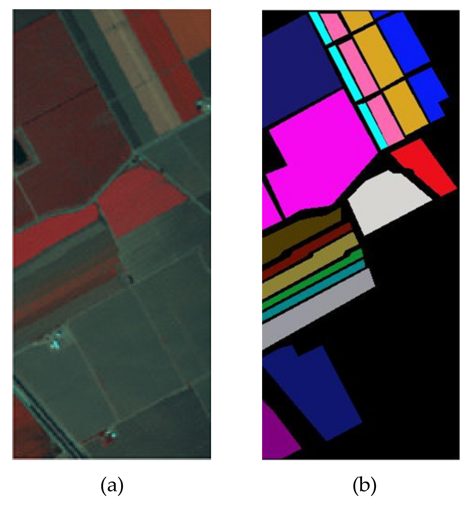
The first data set was captured by the 224-band AVIRIS sensor over Salinas Valley, California. After removing the low signal to noise ratio (SNR) bands, the available data set was composed of 204 bands with 512 × 217 pixels. The ground reference map covers 16 classes of interest. The hyperspectral image is of high spatial resolution (3.7-meter pixels). Figure 5 demonstrates the false-color composite image and the corresponding ground reference map. The number of samples in each class is listed in

Table 3. Land cover classes and numbers of samples in the Salinas data set.

Class			Samples
No.	Color	Name	Numbers
1		Brocoli_green_weeds_1	1977
2		Brocoli_green_weeds_2	3726
3		Fallow	1976
4		Fallow_rough_plow	1394
5		Fallow_smooth	2678
6		Stubble	3959
7		Celery	3579
8		Grapes_untrained	11213
9		Soil_vinyard_develop	6197
10		Corn_senesced_green_weeds	3249
11		Lettuce_romaine_4wk	1058
12		Lettuce_romaine_5wk	1908
13		Lettuce_romaine_6wk	909
14		Lettuce_romaine_7wk	1061
15		Vinyard_untrained	7164
16		Vinyard_vertical_trellis	1737
Total			53785

.

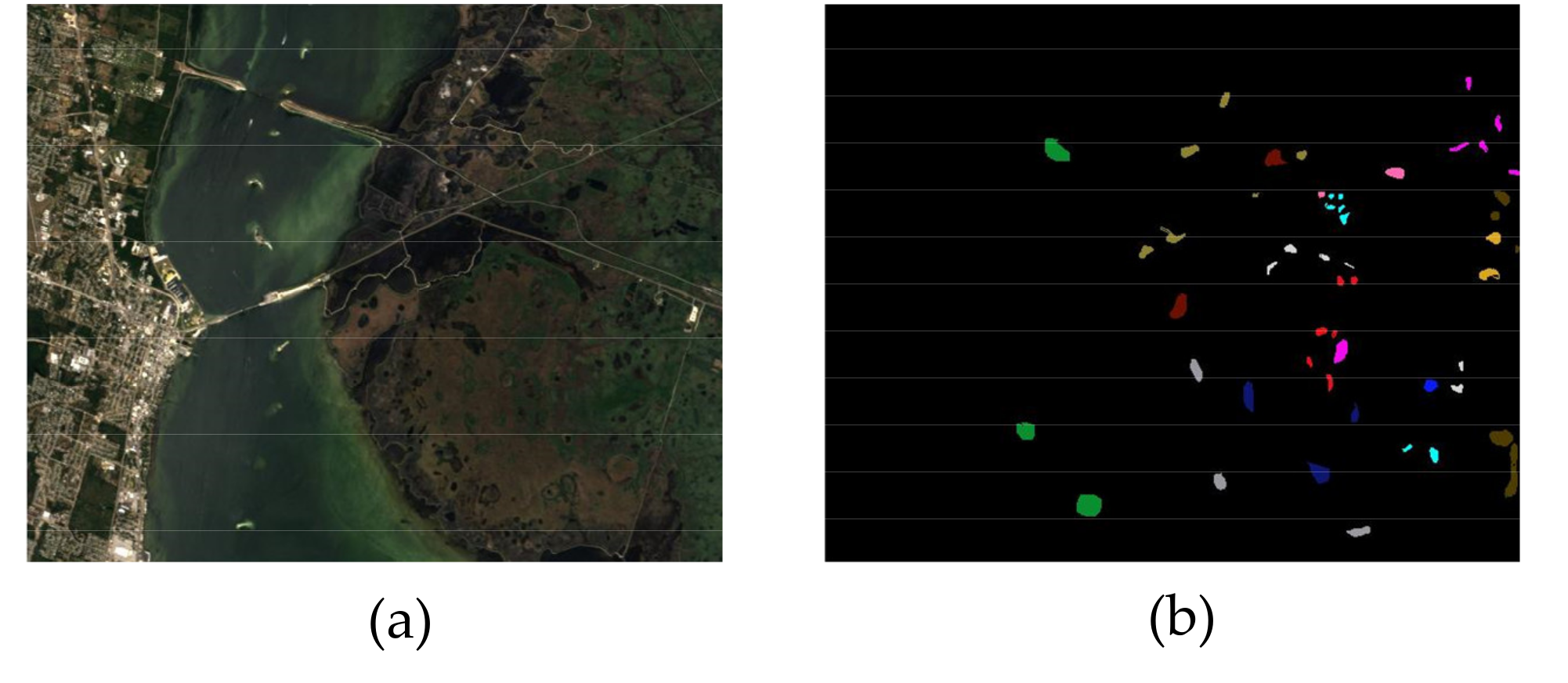
The second data set, KSC, was collected by the airborne AVIRIS instrument over the Kennedy Space Center, Florida. The KSC data set has an altitude of approximately 20 km, with a spatial resolution of 18 m. After removing water absorption and low SNR bands, 176 bands with 512 × 614 pixel vectors were used for the analysis. For classification purpose, 13 classes were selected. The classes of the KSC data set and the corresponding false-color composite map are demonstrated in Figure 6. The number of samples for each class is given in

Table 4. Land cover classes and numbers of samples in the KSC data set.

Class			Samples
No.	Color	Name	Numbers
1		Scrub	761
2		Willow swamp	243
3		CP hammock	256
4		Slash pine	252
5		Oak/Broadleaf	161
6		Hardwood	229
7		Swamp	105
8		Graminoid marsh	431
9		Spartina marsh	520
10		Cattail marsh	404
11		Salt marsh	419
12		Mud flats	503
13		Water	927
Total			5211

.

The third data set is an urban site over the University of Houston campus and neighboring area which was collected by an ITRES-CASI 1500 sensor. The data set is of 2.5-m spatial resolution and consists of 349 × 1905 pixel vectors. The hyperspectral image is composed of 144 spectral bands ranging from 380 to 1050 nm. Fifteen different land-cover classes are provided in the ground reference map, as shown in Figure 7. The samples are listed in

Table 5. Land cover classes and numbers of samples in the Houston data set.

Class			Samples
No.	Color	Name	Numbers
1		Grass Healthy	1251
2		Grass Stresed	1254
3		Grass Synthetic	697
4		Tree	1244
5		Soil	1242
6		Water	325
7		Residential	1268
8		Commercial	1244
9		Road	1252
10		Highway	1227
11		Railway	1235
12		Parking Lot 1	1233
13		Parking Lot 2	469
14		Tennis Court	428
15		Running Track	660
Total			15029

.

For all three data sets, we split the labeled samples into three subsets, i.e., training, validation, and test samples. In our experiment, we randomly chose 200 labeled samples as the training set to train the weights and biases of each neuron and transformation matrix between two consecutive capsule layers. The proper architectures of our network were designed based on performance evaluation on 100 validation samples, which were also randomly chosen from labeled samples. The choice of hyper-parameters, like kernel size in the convolution operation and the dimensions of the vector output of each capsule, were also guided by the validation set. After the training was done, all remaining labeled samples served as the test set to evaluate the capability of the network and to obtain the final classification results. Three evaluation criteria were investigated: overall accuracy (OA), average accuracy (AA), and Kappa coefficients (K).

5.2. The Classification Results of the 1D Capsule Network

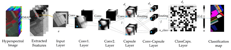
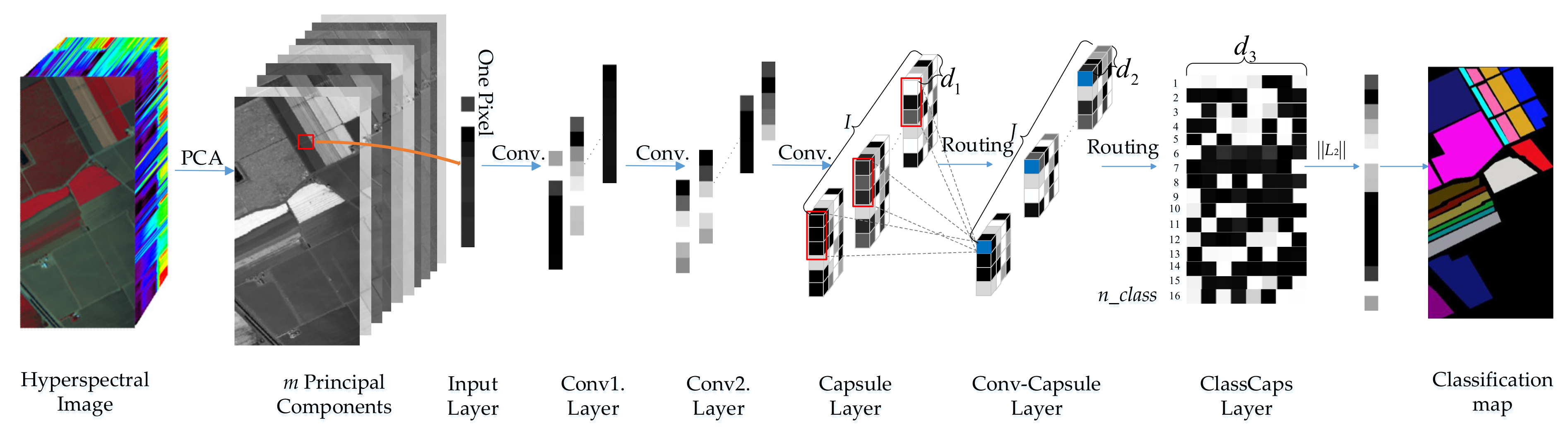
The 1D capsule network, which is built only based on spectral features, contains two parts. One is a fully connected capsule network that uses normalized spectral vectors as input. The other is the Conv-Capsule network which inputs spectral features extracted by PCA. We call the two methods 1D-Capsule and 1D-Conv-Capsule for short. In the 1D-Conv-Capsule, we first used PCA to reduce the spectral dimensions of the data. Then, we randomly chose 200 and 100 labeled samples as the training and validation data for each data set. The training samples were imported to the 1D capsule network. The number of principal components was chosen based on the classification result for the validation samples. Some other hyper-parameters (e.g., the learning rate, the convolutional kernel size, the $\alpha$ in LeakyReLU, etc.) were also determined by the validation set. In our method, the size of the mini-batch was 100 and the number of training epochs was set to 150 for our network. We used a decreasing learning rate which was initialized to 0.01 at the beginning of the training process. The number of the principal components was set to 20, 20, and 30, respectively, for the Salinas, KSC, and Houston data sets. We used $\alpha =0.1$ in the LeakyReLU function. The parameters $m^{+}$, $m^{-}$, and $\lambda$ in the loss function were set to 0.9, 0.1, and 0.5, respectively.

The main architectures of the 1D-Conv-Capsule network for each data set are shown in

Table 6. The architectures of the 1D-Conv-Capsule network for the different data sets.

Nets	No.	Convolution	BN	Stride	Padding	Activation Function
Salinas (KSC)	1	First ten principal components, input shape is 20 × 1 × 1
	2	5 × 1 × 32	YES	1	Yes	LeakyReLU
	3	5 × 1 × 64	YES	1	Yes	LeakyReLU
	4	(5 × 1 × 8) × 8	YES	2	Yes	LeakyReLU, Squash
	5	(5 × 1 × 8) × 16	No	2	No	Squash
	6	Three routing iterations and n_class capsules with a 16-dimensional output vector
Houston	1	First thirty principal components, input shape is 30 × 1 × 1
	2	7 × 1 × 32	YES	1	No	LeakyReLU
	3	7 × 1 × 64	YES	1	No	LeakyReLU
	4	(7 × 1 × 8) × 8	YES	1	No	LeakyReLU, Squash
	5	(3 × 1 × 8) × 16	No	2	No	Squash
	6	Three routing iterations and n_class capsules with a 16-dimensional output vector

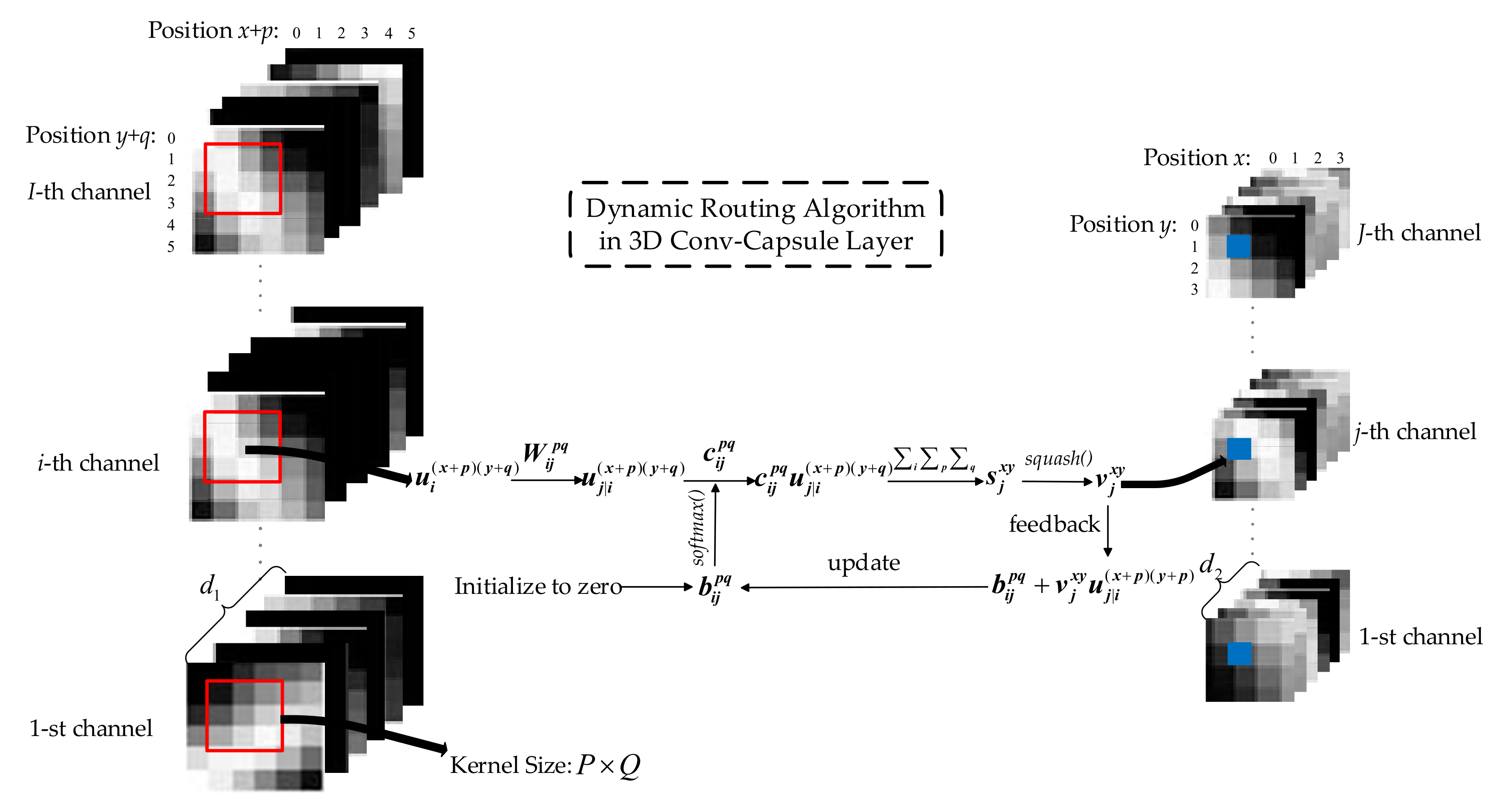
. Due to the fact that the same number of principal components was chosen as the input, the network for the Salinas and KSC data sets had the same architecture. In Table 6, (5 × 1 × 8) × 8 in the fourth layer (i.e., transition layer) means that eight channels of convolution with the kernel size of 5 × 1 were used, and each channel output eight feature maps. Thus, the fourth layer output a capsule with eight channels. The fifth layer was a Conv-Capsule layer with eight (i.e., the number of capsule channels output by the fourth layer) channels of capsule input and 16 channels of capsule output. The kernel size was 5 × 1. We used (5 × 1 × 8) × 16 to represent this operation. The last layer was a fully connected capsule layer. All capsules from the fifth layer were connected with n_class capsules in this layer. The length of the vector output of each capsule in this layer represents the probability of the network’s input belonging to each class. Between consecutive capsule layers in the 1D-Conv-Capsule, three routing iterations were used to determine the coupling coefficients $b_{ij}^p$.

In this set of experiments, our methods were compared with other classical classification methods that are only based on spectral information. These methods included random forest (RF) [47], multiple layer perceptron (MLP) [48], linear support vector machine (L-SVM), support vector machine with the radial basis kernel function (RBF-SVM) [17], recurrent neural network (RNN) [24], and the convolutional neural network (1D-CNN) [28]. Furthermore, 1D-PCA-CNN, which has nearly the same architecture as 1D-Conv-Capsule (apart from the capsule layer), was also designed to give a fair comparison. The classification results are shown in

Table 7. Classification with spectral features on the Salinas data set with different training samples.

Trainin Samples	Method	RF	MLP	L-SVM	RBF-SVM	RNN	1D-CNN	1D-PCA-CNN	1D-Capsule	1D-Conv-Capsule
100	OA (%)	77.81 ± 1.86	80.89 ± 2.25	80.33 ± 2.14	81.01 ± 2.10	71.48 ± 3.50	80.04 ± 1.66	84.07 ± 2.63	77.63 ± 1.52	84.75 ± 1.94
	AA (%)	78.12 ± 3.06	81.56 ± 4.68	79.83 ± 3.58	80.79 ± 4.69	68.84 ± 4.62	80.99 ± 4.08	84.87 ± 4.70	76.41 ± 3.34	86.00 ± 2.01
	K × 100	75.11 ± 2.14	78.68 ± 2.51	78.02 ± 2.44	78.77 ± 2.34	68.26 ± 3.86	77.69 ± 1.87	82.26 ± 2.89	74.92 ± 1.80	83.01 ± 2.15
200	OA (%)	82.63 ± 1.63	84.13 ± 0.50	86.37 ± 1.05	86.07 ± 1.52	79.67 ± 2.42	84.93 ± 0.73	86.52 ± 2.34	83.73 ± 0.23	88.12 ± 1.07
	AA (%)	85.73 ± 2.09	88.71 ± 0.60	89.37 ± 1.92	88.07 ± 2.27	83.22 ± 1.25	89.97 ± 0.58	89.46 ± 3.09	89.02 ± 0.29	91.08 ± 1.70
	K × 100	80.63 ± 1.77	82.21 ± 0.57	84.77 ± 1.18	84.46 ± 1.71	77.38 ± 2.71	83.20 ± 0.82	84.97 ± 2.57	81.78 ± 0.27	86.76 ± 1.21
300	OA (%)	84.24 ± 0.79	87.76 ± 0.83	88.47 ± 0.91	88.22 ± 1.05	81.35 ± 0.90	85.66 ± 1.33	88.46 ± 1.27	84.09 ± 1.36	89.36 ± 0.41
	AA (%)	88.00 ± 1.41	91.72 ± 1.00	91.96 ± 1.16	91.40 ± 1.60	83.88 ± 2.82	88.41 ± 1.98	91.93 ± 1.54	88.28 ± 1.85	92.92 ± 0.32
	K × 100	82.42 ± 0.87	86.37 ± 0.93	87.12 ± 1.02	86.86 ± 1.19	79.20 ± 1.07	84.00 ± 1.48	87.14 ± 1.39	82.22 ± 1.52	88.15 ± 0.44

,

Table 8. Classification with spectral features on the KSC data set with different training samples.

Training Samples	Method	RF	MLP	L-SVM	RBF-SVM	RNN	1D-CNN	1D-PCA-CNN	1D-Capsule	1D-Conv-Capsule
100	OA (%)	73.56 ± 2.63	81.43 ± 1.85	81.38 ± 1.61	80.72 ± 1.85	70.70 ± 2.67	77.19 ± 2.63	81.72 ± 2.02	80.09 ± 1.66	84.83 ± 1.69
	AA (%)	62.52 ± 4.14	72.33 ± 3.58	72.22 ± 3.33	71.17 ± 2.36	58.79 ± 4.74	67.92 ± 3.09	72.41 ± 3.39	70.65 ± 3.16	77.52 ± 3.07
	K × 100	70.49 ± 2.95	79.30 ± 2.06	79.25 ± 1.79	78.51 ± 2.05	67.30 ± 3.07	74.57 ± 2.94	79.63 ± 2.26	77.79 ± 1.86	83.09 ± 1.87
200	OA (%)	80.08 ± 1.12	85.15 ± 0.81	86.35 ± 1.50	86.64 ± 1.21	82.03 ± 1.33	84.80 ± 0.97	86.02 ± 2.16	84.39 ± 0.33	88.22 ± 1.06
	AA (%)	71.52 ± 1.93	78.78 ± 0.98	78.06 ± 2.76	79.57 ± 1.76	74.68 ± 1.21	79.32 ± 1.48	78.91 ± 2.97	78.66 ± 0.36	82.11 ± 2.52
	K × 100	77.79 ± 1.26	83.45 ± 0.90	84.78 ± 1.68	85.11 ± 1.35	79.97 ± 1.48	83.08 ± 1.08	84.44 ± 2.39	82.59 ± 0.37	86.87 ± 1.18
300	OA (%)	82.31 ± 0.98	88.02 ± 0.67	88.56 ± 0.84	88.87 ± 0.93	82.35 ± 1.81	84.34 ± 1.12	88.03 ± 0.88	85.81 ± 1.40	89.84 ± 1.41
	AA (%)	75.32 ± 0.99	82.15 ± 1.55	82.45 ± 2.23	83.55 ± 1.39	73.33 ± 3.10	78.37 ± 1.84	81.45 ± 2.09	79.11 ± 1.29	84.43 ± 2.29
	K × 100	80.26 ± 1.09	86.66 ± 0.75	87.27 ± 0.95	87.60 ± 1.04	80.33 ± 2.02	82.56 ± 1.25	86.66 ± 0.99	84.18 ± 1.55	88.68 ± 1.57

and

Table 9. Classification with spectral features on the Houston data set with different training samples.

Training Samples	Method	RF	MLP	L-SVM	RBF-SVM	RNN	1D-CNN	1D-PCA-CNN	1D-Capsule	1D-Conv-Capsule
100	OA (%)	64.68 ± 2.27	72.42 ± 1.39	69.89 ± 1.99	72.95 ± 1.64	62.41 ± 3.10	70.66 ± 3.43	72.51 ± 2.94	70.11 ± 3.14	76.04 ± 1.90
	AA (%)	63.59 ± 3.34	70.82 ± 2.88	70.11 ± 2.28	72.03 ± 2.23	61.58 ± 2.96	68.20 ± 3.99	71.43 ± 3.81	69.64 ± 4.34	75.46 ± 2.93
	K × 100	61.76 ± 2.47	70.15 ± 1.52	67.42 ± 2.16	70.73 ± 1.77	59.37 ± 3.36	68.22 ± 3.73	70.24 ± 3.18	67.66 ± 3.41	74.08 ± 2.06
200	OA (%)	72.64 ± 1.27	80.69 ± 1.53	75.47 ± 0.96	78.91 ± 0.95	74.24 ± 1.61	79.47 ± 0.59	80.85 ± 1.55	77.54 ± 2.47	84.06 ± 1.34
	AA (%)	71.48 ± 1.54	79.68 ± 1.88	75.22 ± 1.11	78.06 ± 0.91	73.22 ± 1.45	77.94 ± 1.59	80.62 ± 1.59	77.39 ± 1.99	83.46 ± 1.43
	K × 100	70.39 ± 1.37	79.11 ± 1.65	73.45 ± 1.04	77.17 ± 1.03	72.15 ± 1.73	77.80 ± 0.64	79.29 ± 1.69	75.70 ± 2.67	82.75 ± 1.46
300	OA (%)	77.32 ± 1.17	83.25 ± 1.36	79.00 ± 1.51	83.30 ± 1.17	77.61 ± 2.36	79.26 ± 1.13	86.39 ± 0.37	80.25 ± 1.19	87.11 ± 1.38
	AA (%)	75.99 ± 1.03	82.32 ± 1.49	77.97 ± 1.33	82.16 ± 1.25	75.79 ± 1.71	78.18 ± 1.57	85.47 ± 0.93	79.37 ± 1.19	86.32 ± 1.50
	K × 100	75.45 ± 1.26	81.87 ± 1.47	77.26 ± 1.63	81.93 ± 1.26	75.80 ± 2.53	77.55 ± 1.23	85.27 ± 0.40	78.63 ± 1.29	86.06 ± 1.50

.

The experiment setups of the classical classification methods are described as follows. RF was used for classification. A grid search method and four-fold cross-validation were used to define RF’s two key hyper-parameters (i.e., the number of features to consider when looking for the best split (F) and the number of trees (T)). In the experiment, the search ranges of F and T were (5, 10, 15, 20) and (100, 200, 300, 400), respectively. The MLP used in this experiment was a fully connected neural network with one hidden layer. The used MLP contained 64 hidden units. L-SVM is a linear SVM with no kernel function. RBF-SVM uses the radial basis function as the kernel. In L-SVM and RBF-SVM, a grid search method and four-fold cross-validation were also used to define the most appropriate hyper-parameters (i.e., $C$ for L-SVM and $\left(C,\gamma \right)$ for RBF-SVM). In this experiment, the search range was exponentially growing sequences of $C$ and $\gamma$ ($C={10}^{-3},{10}^{-2},\dots ,{10}^3$, $\gamma ={10}^{-3},{10}^{-2},\dots ,{10}^3$). A single layer RNN with a gated recurrent unit and the tanh activation function were adopted. The architecture of 1D-CNN was designed as in [28] and contained an input layer, a convolutional layer, a max-pooling layer, a fully connected layer, and an output layer. The convolutional kernel size and number of kernels were 17 and 20 for all three data sets. The pooling size was 5, 5, and 4 for the Salinas, KSC, and Houston data sets, respectively. Table 7, Table 8 and Table 9 show the classification results obtained when we used the aforementioned experimental settings. All experiments were run ten times with different random training samples. The classification accuracy is given in the form of mean ± standard deviation. The 1D-Conv-Capsule network showed a better performance in terms of accuracy on all three data sets.

For all three data sets, RBF-SVM, which is famous for handling a limited number of training samples, provides competitive classification results. We use the experiments with 200 training samples as an example to discuss the results. For the Salinas data set, 1D-Conv-Capsule exhibited the best OA, AA, and K, with improvements of 2.05%, 3.01%, and 0.023 over RBF-SVM, respectively. Our approach outperformed 1D-PCA-CNN by 1.6%, 1.62%, and 0.0179 in terms of OA, AA, and K, respectively. For the KSC data set, as can be seen, the OA of 1D-Conv-Capsule was 88.22%, which is an increase of 1.58% and 2.2% compared with RBF-SVM and 1D-PCA-CNN, respectively. For the Houston data set, 1D-Conv-Capsule improved the OA, AA, and K of 1D-PCA-CNN by 3.21%, 2.84%, and 0.0346, respectively. The results show that the 1D-Conv-Capsule method demonstrated the best performance in terms of OA, AA, and K for all three data sets. In addition, all experiments with 100 and 300 training samples were also implemented to demonstrate the effectiveness of the proposed methods. From the results reported in Table 7, Table 8 and Table 9, it can be seen that 1D-Conv-Capsule outperformed the other classical classification methods, especially when the number of training samples was extremely limited (i.e., 100 training samples).

Furthermore, the 1D-Conv-Capsule with a different number of principal components as input was conducted. Figure 8 shows the classification results of the 1D-Conv-Capsule on three data sets by using 200 training samples. Due to the fact that we injected only spectral information into the 1D-Conv-Capsule, relatively more principal components were used to make sure that sufficient spectral information was preserved, and, at the same time, this maintained low computational complexity. From Figure 8, it can be seen that if the number of selected components is too small or too big, the classification results tend to be poor under both circumstances. On one hand, the spectral information is not sufficiently preserved and the network cannot efficiently extract the spectral feature when the number of principal components is low. On the other hand, the networks are over-trained when the number of principal components is high. The situation becomes worse if the number of training samples is limited. The best classification performance was achieved when the number of the principal components was set to 20, 20, and 30 for the Salinas, KSC, and Houston data sets, respectively.

5.3. The Analysis of Learnt Features of the 1D Capsule

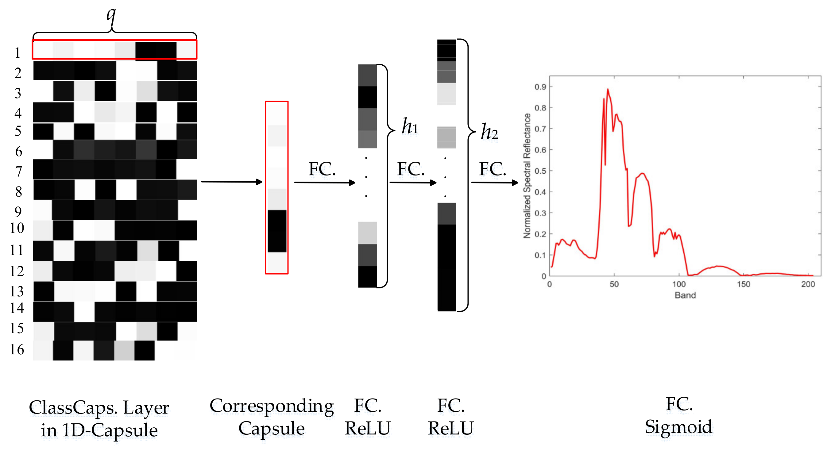
From the aforementioned description about the capsule, it can be understood that the output of the capsule is a vector representation of the type of entity. In order to demonstrate the real advantage of the capsule network on remote sensing data, we performed another experiment based on the 1D-Capsule network followed by a reconstruction network (1D-Capsule-Recon). The architecture of the reconstruction network is shown in Figure 9. According to the label of the input pixel, the representative vector of the corresponding capsule in the ClassCaps layer was imported to the reconstruction network (e.g., if the input pixel belonged to the $i$-th class, the vector output of the $i$-th capsule in the ClassCaps layer was used as input to the reconstruction network). The reconstruction network contained three fully connected (FC) layers. The first two FC layers had 128 and 256 hidden units with the ReLU activation function. The last FC layer with Sigmoid activation function output the reconstructed spectra (i.e., a combination of normalized spectral reflectance of different bands) corresponding to the input of the 1D-Capsule-Recon. The reconstruction loss, i.e., the Euclidean distance between the input and the reconstructed spectra, was added to the margin loss that described in Section 3:

L_total = L_M + εL_R,

(18)

where $L_M$ is the margin loss and $L_R$ is the reconstruction loss. $\epsilon$ is the weight coefficient that is used to avoid $L_R$ dominating $L_M$ during the training procedure. In the experiment, $\epsilon$ was set to 0.1. $L_{total}$ was used as the loss function for the 1D-Capsule-Recon.

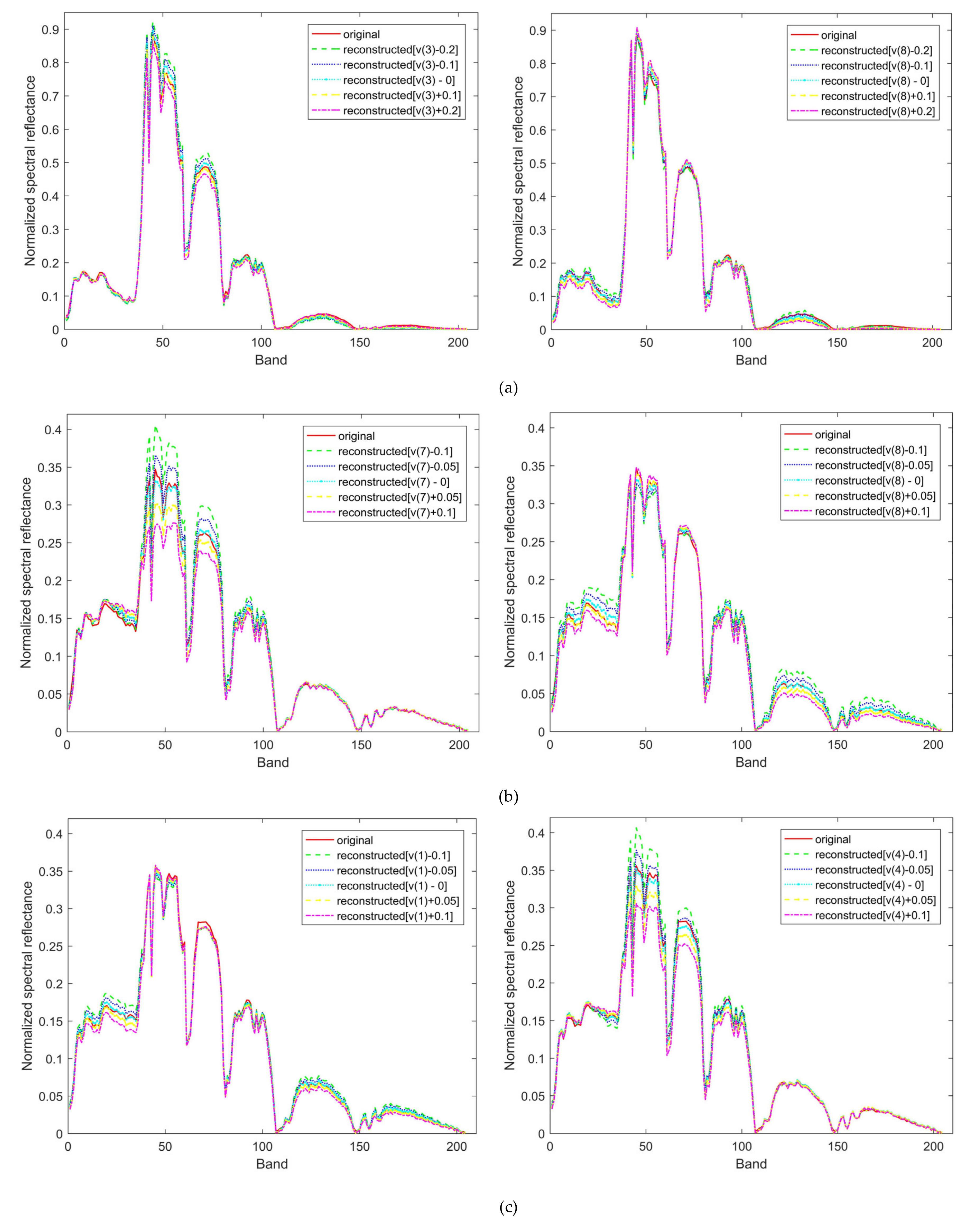
To visualize the vector representation of the capsule, we made use of the reconstruction network. After the training procedure of the 1D-Capsule-Recon was done, we randomly chose some samples from different classes and computed the representation vector of their corresponding capsules in the ClassCaps layer. We made perturbations in different dimensions of the vector and fed them to the reconstruction network. Figure 10 shows the reconstructed results of three class samples from the Salinas data set. Two dimensions of the representation vector were tuned. In Figure 10, the original is the input spectra to the 1D-Capsule-Recon. The notation of [$v\left(i\right)+\mathsf{\Delta }$] in Figure 10 means that we tuned the $i$-th dimension of the representation vector $v$ with perturbation $\mathsf{\Delta }$. The perturbed $v$ was used to reconstruct the spectra. From the results shown in Figure 10, the representation vector (i.e., $v$) can well reconstruct the spectra, which means that the representation vector contains the information in the spectra with low dimensionality.

Furthermore, as shown in Figure 10, $v\left(i\right)+\mathsf{\Delta }$ can influence the reconstruction of some special bands, which means that $v\left(i\right)$ has a close relationship with the special bands. $v$ is a vector that contains several $v\left(i\right)$, and $v$ is a robust and condensed representation of spectra.

5.4. The Classification Results of the 3D Capsule Network

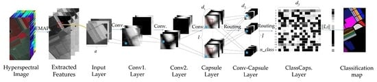
In the 3D capsule network, the network extracts both spectral and spatial features effectively, which could lead to a better performance in terms of classification accuracy than the one obtained by the 1D capsule network. As mentioned above, we proposed two 3D frameworks, i.e., the 3D-Capsule and the 3D-Conv-Capsule. Similar to a 1D framework, the 3D-Capsule is an original fully connected capsule network, while the 3D-Conv-Capsule is the convolutional capsule network. Additionally, the 3D-Capsule directly uses the original hyperspectral data as input, while the 3D-Conv-Capsule utilizes EMAP to extract features of hyperspectral data. In the 3D-Conv-Capsule, three principal components were used and parameters in EMAP were set as in [21]. Through the EMAP analysis, the number of spectral dimensions became 108 for all three data sets. In this set of experiments, the numbers of training and validation samples were the same as for the 1D Capsule network. The mini-batch size was also 100. The training epoch was set to 100 with a learning rate of 0.001. The parameter in loss function was the same as for the 1D capsule network. The details on the architecture of the 3D-Conv-Capsule network are shown in

Table 10. The architectures of the 3D-Conv-Capsule network.

Nets	No.	Convolution	BN	Stride	Padding	Activation Function
Salinas KSC Houston	1	Features extracted by EMAP, input shape is 27 × 27 × 108
	2	3 × 3 × 32	YES	1	No	ReLU
	3	3 × 3 × 64	YES	1	No	ReLU
	4	(4 × 4 × 8) × 4	YES	2	No	ReLU, Squash
	5	(3 × 3 × 4) × 8	No	2	No	Squash
	6	Three routing iterations and n_class capsules with a 16-dimensional output vector

. The definitions of the parameters in Table 10 can be found in the description for the 1D-Conv-Capsule network. Batch normalization was also used to improve the performance of the network.

The SVM-based and CNN-based methods were included in the experiments to give a comprehensive comparison. The classification results are shown in

Table 11. Classification with spectral-spatial features on the Salinas data set with different training samples.

Training Samples	Method	EMP-SVM	EMP-CNN	EMAP-RF	EMAP-SVM	3D-CNN	SSRN [49]	3D-EMAP-CNN	3D-Capsule	3D-Conv-Capsule
100	OA (%)	86.13 ± 2.21	84.28 ± 0.97	87.33 ± 2.44	90.15 ± 2.42	82.34 ± 2.47	84.40 ± 2.11	86.58 ± 4.60	88.00 ± 2.53	93.96 ± 2.18
	AA (%)	86.40 ± 4.96	77.50 ± 4.11	85.11 ± 4.97	91.22 ± 4.07	79.05 ± 2.78	80.90 ± 4.92	82.24 ± 4.80	83.37 ± 4.23	88.03 ± 4.31
	K × 100	84.49 ± 2.53	82.29 ± 1.11	85.88 ± 2.73	89.02 ± 2.72	80.11 ± 2.85	82.52 ± 2.41	84.95 ± 5.07	86.54 ± 2.83	93.25 ± 2.43
200	OA (%)	90.07 ± 1.45	92.71 ± 0.66	94.27 ± 1.14	94.72 ± 2.04	90.68 ± 1.28	91.16 ± 1.64	94.28 ± 2.14	94.86 ± 1.63	97.92 ± 0.30
	AA (%)	91.42 ± 2.30	93.22 ± 0.62	93.45 ± 2.41	95.35 ± 3.21	88.18 ± 1.25	93.59 ± 2.35	92.86 ± 3.32	93.49 ± 3.15	96.21 ± 1.87
	K × 100	88.93 ± 1.63	91.83 ± 0.74	93.62 ± 1.26	94.12 ± 2.29	89.56 ± 1.45	90.16 ± 1.82	93.59 ± 2.41	94.24 ± 1.83	97.68 ± 0.34
300	OA (%)	91.92 ± 0.40	94.91 ± 1.04	95.66 ± 1.02	96.35 ± 0.54	93.98 ± 1.34	92.81 ± 1.21	98.41 ± 0.77	97.64 ± 1.00	99.17 ± 0.58
	AA (%)	94.22 ± 0.44	94.60 ± 1.77	95.77 ± 1.87	97.22 ± 0.61	92.79 ± 2.57	95.20 ± 1.18	98.44 ± 1.01	97.27 ± 1.33	98.95 ± 0.73
	K × 100	91.00 ± 0.45	94.30 ± 1.18	95.18 ± 1.14	95.94 ± 0.60	93.25 ± 1.52	91.98 ± 1.35	98.23 ± 0.86	97.36 ± 1.12	99.07 ± 0.65

,

Table 12. Classification with spectral-spatial features on the KSC data set with different training samples.

Training Samples	Method	EMP-SVM	EMP-CNN	EMAP-RF	EMAP-SVM	3D-CNN	SSRN [49]	3D-EMAP-CNN	3D-Capsule	3D-Conv-Capsule
100	OA (%)	87.83 ± 2.04	86.95 ± 1.68	85.44 ± 2.15	87.88 ± 3.14	84.15 ± 2.58	90.79 ± 2.83	90.07 ± 3.05	88.42 ± 1.23	93.23 ± 2.50
	AA (%)	81.80 ± 3.19	80.63 ± 2.09	78.34 ± 4.16	81.93 ± 3.95	76.98 ± 4.00	84.09 ± 6.20	84.97 ± 5.02	82.28 ± 3.42	89.10 ± 3.94
	K × 100	86.43 ± 2.27	85.46 ± 1.87	83.71 ± 2.42	86.49 ± 3.51	82.35 ± 2.88	89.73 ± 3.17	88.95 ± 3.41	87.12 ± 1.37	92.47 ± 2.78
200	OA (%)	93.63 ± 1.77	96.56 ± 1.24	91.81 ± 1.30	93.66 ± 0.95	95.98 ± 0.85	96.77 ± 0.83	95.30 ± 0.96	97.08 ± 0.41	98.75 ± 0.87
	AA (%)	90.28 ± 2.68	94.65 ± 2.48	87.52 ± 1.75	90.89 ± 1.77	94.07 ± 1.39	94.70 ± 0.86	92.36 ± 1.25	95.77 ± 0.58	98.01 ± 1.36
	K × 100	92.90 ± 1.98	96.18 ± 1.38	90.86 ± 1.44	92.94 ± 1.07	95.53 ± 0.95	96.41 ± 0.93	94.77 ± 1.06	96.75 ± 0.45	98.62 ± 0.97
300	OA (%)	95.34 ± 1.09	98.29 ± 0.83	94.43 ± 0.79	95.28 ± 0.99	97.69 ± 0.69	98.21 ± 0.69	98.57 ± 0.91	98.21 ± 1.07	99.19 ± 0.63
	AA (%)	93.12 ± 1.59	97.45 ± 1.48	91.81 ± 1.05	92.91 ± 2.43	96.66 ± 1.17	96.30 ± 1.50	97.58 ± 1.53	97.27 ± 1.49	98.35 ± 1.51
	K × 100	94.81 ± 1.22	98.10 ± 0.93	93.79 ± 0.88	94.75 ± 1.10	97.44 ± 0.77	98.01 ± 0.77	98.41 ± 1.01	98.01 ± 1.19	99.10 ± 0.70

and

Table 13. Classification with spectral-spatial features on the Houston data set with different training samples.

Training Samples	Method	EMP-SVM	EMP-CNN	EMAP-RF	EMAP-SVM	3D-CNN	SSRN [49]	3D-EMAP-CNN	3D-Capsule	3D-Conv-Capsule
100	OA (%)	79.39 ± 2.63	71.35 ± 2.59	76.57 ± 4.43	78.82 ± 1.74	70.29 ± 4.07	74.58 ± 3.64	73.51 ± 2.80	77.96 ± 3.49	82.61 ± 2.83
	AA (%)	77.13 ± 4.67	67.57 ± 3.46	75.32 ± 4.53	76.75 ± 2.61	67.77 ± 4.83	75.19 ± 3.91	70.60 ± 3.45	76.04 ± 3.77	80.82 ± 3.86
	K × 100	77.69 ± 2.86	68.97 ± 2.81	74.64 ± 4.80	77.07 ± 1.89	67.82 ± 4.41	72.51 ± 3.94	71.31 ± 3.05	76.16 ± 3.78	81.18 ± 3.08
200	OA (%)	86.63 ± 1.26	85.46 ± 2.05	85.68 ± 1.86	87.20 ± 1.51	85.19 ± 1.95	85.12 ± 1.49	87.54 ± 1.92	88.69 ± 1.92	90.41 ± 1.28
	AA (%)	86.29 ± 2.19	85.40 ± 1.95	85.30 ± 1.80	86.63 ± 1.87	83.11 ± 2.74	85.47 ± 1.39	85.43 ± 1.96	86.83 ± 2.75	89.46 ± 1.72
	K × 100	85.54 ± 1.36	84.29 ± 2.21	84.51 ± 2.01	86.17 ± 1.63	83.98 ± 2.11	83.90 ± 1.62	86.52 ± 2.07	87.77 ± 2.08	89.63 ± 1.38
300	OA (%)	90.44 ± 1.34	89.76 ± 1.97	90.17 ± 0.93	90.52 ± 0.75	90.02 ± 1.02	90.64 ± 1.97	91.78 ± 1.48	92.55 ± 1.32	94.16 ± 1.62
	AA (%)	90.10 ± 1.77	89.74 ± 2.78	90.12 ± 1.09	89.75 ± 1.27	89.19 ± 1.68	91.00 ± 1.90	92.19 ± 1.41	91.87 ± 1.86	93.73 ± 2.32
	K × 100	89.66 ± 1.45	88.93 ± 2.13	89.37 ± 1.01	89.74 ± 0.81	89.21 ± 1.10	89.88 ± 2.13	91.11 ± 1.60	91.94 ± 1.43	93.69 ± 1.76

. For the three data sets, we used 27 × 27 neighbors of each pixel as input 3D images in these methods.

Due to the high performance in terms of classification accuracy of SVM, some SVM-based HSIs classifiers were adopted for comparison. The extended morphological profile with SVM (EMP-SVM) is a widely used spectral-spatial classifier [19]. In the EMP-SVM method, the morphological opening and closing operations were used to extract spatial information on the first three components of HSIs, which were computed by PCA. In the experiments, the shape structuring element (SE) was set as a disk, and the radius of disk increased from two to eight with an interval of two. Therefore, 27 spatial features were generated. The learned features were fed to an RBF-SVM to obtain the final classification results. EMAP is a generalization of the EMP and can extract more informative spatial information. EMAP was also combined with the random forest classifier (EMAP-RF) [20]. In order to have a fair comparison, the parameters in EMAP were kept the same as for the 3D-Conv-Capsule. In RBF-SVM, the optimal parameters $C$ and $\gamma$ were also obtained by grid-search and four-fold cross-validation methods. Furthermore, CNN was also used for comparison. We conducted 3D-CNN, EMP-CNN and 3D-EMAP-CNN. Their CNN architectures were the same as in [31]. To give a comprehensive comparison, a spectral–spatial residual network recently proposed in [49] was adopted for comparison.

Table 11, Table 12 and Table 13 give the classification results of the proposed methods and contrast methods on the three data sets. We also used the classification results with 200 training samples as an example. For the Salinas data set, the 3D-Conv-Capsule exhibited the highest OA, AA, and K, with the improvements of 3.64%, 3.35%, and 0.0409 over 3D-EMAP-CNN, respectively. On the other hand, our 3D-Capsule approach also performed better than 3D-EMAP-CNN in terms of OA, AA, and K. For the KSC data set, 3D-Conv-Capsule improved the OA, AA, and K of EMP-CNN by 2.19%, 3.36%, and 0.0244, respectively. Our 3D-Capsule method also showed higher classification accuracy than EMP-CNN with improvements of 0.52%, 1.12%, and 0.0057 in terms of OA, AA, and K. For the Houston data set, we obtained similar results. Experiments with 100 and 300 training samples were investigated as well. The detailed classification results are shown in Table 11, Table 12 and Table 13. Compared with other state-of-the-art methods, the 3D-Conv-Capsule demonstrated the best performance under different training samples.

In the experiment using the 3D-Conv-Capsule, we also explored how a different number of principal components that are used in EMAP analysis may affect the classification results. Due to the spatial information being considered and the EMAP analysis significantly increasing the data volume, we used relatively fewer principal components here compared with the 1D-Conv-Capsule. Figure 11 shows the classification result for the 3D-Conv-Capsule. The 3D-Conv-Capsule with different numbers of principal components outperformed the other contrast experiments. Unlike 1D-Conv-Capsule, the preservation of more principal components leads to a vast data volume which brings a higher requirement for hardware and longer training time in 3D-Conv-Capsule. Though the classification accuracy may be higher with relatively more components, we only used three principal components in consideration of computational cost in the 3D-Conv-Capsule.

5.5. Parameter Analysis

In the 3D-Conv-Capsule, convolutional layers were used as feature extractors, and they converted the original input into a capsule’s input. Thus, the number of convolutional layers and the convolutional kernel size used in 3D-Conv-Capsule influences the classification performance of the model. Furthermore, due to the fact that the input of a 3D-Conv-Capsule is the a × a neighbors around the pixel, the size of neighborhoods is also an important factor. These factors are analyzed below.

When we explored the influence of a parameter on the classification result, the other parameters were fixed. The neighborhood size and convolution kernel size were set to 27 and 3 when we analyzed the number of convolutional layers. For the analysis of the convolution kernel size, 27 × 27 neighborhoods and two convolutional layers were used in the 3D-Conv-Capsule. Similarly, the number of convolutional layers and the convolution kernel size were set to 2 and 3 for analysis of the size of the neighborhood. All the experiments for this analysis were conducted with 200 training samples.

Table 14. Classification results of the 3D-Conv-Capsule with different numbers of convolutional layers on three data sets.

Data Set	Convolutional Layers	1	2	3
Salinas	OA (%)	97.60 ± 1.12	97.92 ± 0.30	97.69 ± 0.77
	AA (%)	95.69 ± 2.77	96.21 ± 1.87	95.84 ± 2.45
	K × 100	97.32 ± 1.25	97.68 ± 0.34	97.41 ± 0.87
KSC	OA (%)	97.80 ± 1.20	98.75 ± 0.87	98.20 ± 1.24
	AA (%)	96.53 ± 2.10	98.01 ± 1.36	97.08 ± 2.09
	K × 100	97.55 ± 1.33	98.62 ± 0.97	97.99 ± 1.37
Houston	OA (%)	88.86 ± 1.58	90.41 ± 1.28	89.04 ± 1.17
	AA (%)	88.03 ± 2.80	89.46 ± 1.72	86.94 ± 1.84
	K × 100	87.96 ± 1.72	89.63 ± 1.38	88.15 ± 1.27

,

Table 15. Classification results of the 3D-Conv-Capsule with different convolutional kernel sizes on three data sets.

Data Set	Kernel Size	3	5	7
Salinas	OA (%)	97.92 ± 0.30	97.08 ± 1.21	97.39 ± 0.84
	AA (%)	96.21 ± 1.87	95.59 ± 3.77	96.90 ± 2.05
	K × 100	97.68 ± 0.34	96.73 ± 1.35	97.08 ± 0.95
KSC	OA (%)	98.75 ± 0.87	97.39 ± 1.10	98.25 ± 1.19
	AA (%)	98.01 ± 1.36	95.68 ± 1.65	97.26 ± 1.85
	K × 100	98.62 ± 0.97	97.10 ± 1.22	98.05 ± 1.32
Houston	OA (%)	90.41 ± 1.28	88.40 ± 1.28	89.06 ± 1.77
	AA (%)	89.46 ± 1.72	87.71 ± 2.72	87.84 ± 1.89
	K × 100	89.63 ± 1.38	87.46 ± 1.38	88.18 ± 1.91

and

Table 16. Classification result of the 3D-Conv-Capsule with different neighborhood sizes on three data sets.

Data Set	Neighborhoods	11	17	21	27
Salinas	OA (%)	95.73 ± 0.87	96.65 ± 2.11	97.07 ± 0.81	97.92 ± 0.30
	AA (%)	95.52 ± 2.98	95.34 ± 4.28	96.15 ± 1.06	96.21 ± 1.87
	K × 100	95.24 ± 0.97	96.25 ± 2.36	96.73 ± 0.90	97.68 ± 0.34
KSC	OA (%)	97.36 ± 0.81	97.68 ± 1.18	97.46 ± 1.15	98.75 ± 0.87
	AA (%)	95.69 ± 1.30	96.34 ± 1.75	94.92 ± 3.42	98.01 ± 1.36
	K × 100	97.07 ± 0.90	97.42 ± 1.30	97.18 ± 1.27	98.62 ± 0.97
Houston	OA (%)	91.56 ± 0.87	91.35 ± 0.78	91.08 ± 1.30	90.41 ± 1.28
	AA (%)	91.81 ± 1.43	89.92 ± 0.70	90.10 ± 1.89	89.46 ± 1.72
	K × 100	90.88 ± 0.94	90.65 ± 0.84	90.36 ± 1.41	89.63 ± 1.38

shows the detailed classification results. As reported in Table 14, the use of two convolutional layers gave better classification results. Furthermore, one convolutional layer could not extract features efficiently while three layers made the model prone to overfitting. Table 15 shows the classification results with different convolution kernel sizes. The 3D-Conv-Capsule performed better when the kernel size was 3. For the neighborhood size, the 3D-Conv-Capsule obtained good classification accuracies on the Salinas and KSC data sets when the neighborhood size was relatively large, but the result for the Houston data set was the other way around.

5.6. Visualization of Learnt Features from the Capsule Network

Unlike traditional neural networks which use a sequence of scalar value to represent the probability of the input belonging to different classes, capsule networks output n_class (i.e., the number of classes) capsules that represent different classes of entity. The length of the vector output of each capsule (i.e., the Euclidean norm of the vector) represents the probability that a corresponding entity exists. In HSI classification tasks, the length of different capsules’ output vectors can be interpreted as the probability that the input belongs to different classes.

We randomly choose several samples from the test data set and imported them into the trained 3D-Conv-Capsule network. The length of the vector output of each capsule in the ClassCaps layer is computed and visualized in Figure 12. From the results shown in Figure 12, it is possible to observe that the capsule corresponding to the true class output the longest vector. Due to the similarity between the Graminoid marsh and Spartina marsh, the experimental results of three samples from the Graminoid marsh class show that the length of the vector corresponding to the similar class was longer than those of the other classes.

5.7. Time Consumption

All experiments in this paper were conducted on a Dell laptop equipped with an Intel Core i5-7300H processor with 2.5 GHz, 8 GB of DDR4 RAM, and an NVIDIA GeForce GTX 1050Ti graphical processing unit (GPU). The software environment used Windows 10 as an operating system, CUDA 9.0 and cuDNN 7.1, Keras framework using TensorFlow as a backend, and Python 3.6 as the programing language. The training and test times of different models are reported in

Table 17. Training and test times of different spectral classifiers for the three HSI data sets with 200 training samples.

	Methods	RF	MLP	L-SVM	RBF-SVM	RNN	1D-CNN	1D-PCA-CNN	1D-Capsule	1D-Conv-Capsule
Data Sets
Salinas	Train (s)	23.5	6.8	0.43	4.8	190.3	19.5	17.1	230.3	92.2
	Test (s)	1.5	0.2	1.5	1.65	4.1	0.29	0.25	120.5	56.3
KSC	Train (s)	21.0	6.5	0.37	4.4	160.2	19.1	17.5	160.2	88.5
	Test (s)	0.2	0.04	0.11	0.13	2.1	0.02	0.02	8.2	5.2
Houston	Train (s)	26.0	6.5	0.49	4.0	135.1	17.5	17.7	145.3	110.2
	Test (s)	0.5	0.07	0.36	0.45	3.5	0.07	0.07	22.3	16.8

and

Table 18. Training and test times of different spectral-spatial classifiers for the three HSI data sets with 200 training samples.

	Methods	EMP-SVM	EMP-CNN	EMAP-RF	EMAP-SVM	3D-CNN	SSRN	3D-EMAP-CNN	3D-Capsule	3D-Conv-Capsule
Data Sets
Salinas	Train (s)	1.1	32.5	18.7	2.95	130.2	240.3	72.2	270.2	140.2
	Test (s)	0.38	3.7	1.5	0.8	19.2	43.6	28.4	220.4	128.4
KSC	Train (s)	1.0	28	19.1	2.75	122.3	215.5	72.1	240.1	140.1
	Test (s)	0.04	0.4	0.15	0.08	1.5	3.8	1.0	17.6	12.3
Houston	Train (s)	1.2	45.0	22.2	3.2	133	190.2	75.2	255.7	135.2
	Test (s)	0.13	1.2	0.5	0.31	3.0	9.0	4.9	65.2	36.1

. The traditional RF and SVM classifiers demonstrated superior computational efficiency. As for deep learning models, the model was able to be trained within a few minutes due to the limited number of training samples and the GPU’s strong computing acceleration power. The 3D-Conv-Capsule required nearly the same training time as 3D-CNN and less time than SSRN. In the experiments, it was found that capsule network-based method converged “faster” than the CNN-based method (e.g., 100 epochs for 3D-Conv-Capsule and 500 epochs for 3D-EMAP-CNN). In future work, the use of more specific computing acceleration for the capsule network could further boost the computational efficiency of the capsule-based method.

5.8. Classification Maps

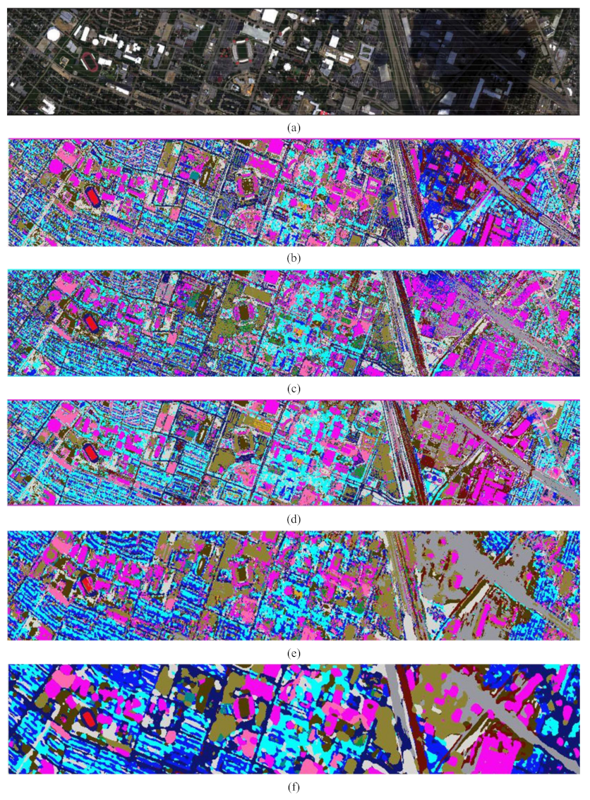
Lastly, we evaluated the classification accuracies from a visual perspective. The trained models, including 1D-CNN, 1D-Conv-Capsule, EMAP-SVM, 3D-CNN and 3D-Conv-Capsule, were selected to classify the whole images. All parameters in these models were optimized. Figure 13, Figure 14 and Figure 15 show the classification maps obtained by different models using the three data sets. From Figure 13, Figure 14 and Figure 15, we can figure out how the different classification methods affect the classification results. Although the 1D-Conv-Capsule demonstrated a higher accuracy than 1D-CNN, the 1D-CNN and 1D-Conv-Capsule models, which only utilize spectral features, depicted more errors compared with spectral-spatial-based methods for the three data sets. Spectral-based models always result in noisy scatter points in the classification map (see Figure 13b,c, Figure 14b,c and Figure 15b,c). Spectral-spatial methods overcome this shortcoming. Obviously, 3D-CNN and 3D-Conv-Capsule, which directly use the neighbor information as the model input, resulted in smoother classification maps. By comparing the true ground reference with the classification maps, the 3D-Conv-Capsule obtained more precise classification results, which demonstrates that the capsule network is an effective method for HSI classification.

6. Conclusions

In this paper, an improved capsule network called the convolutional capsule (Conv-Capsule) was proposed. On the basis of Conv-Capsule, new deep models called 1D-Conv-Capsule and 3D-Conv-Capsule were investigated for HSI classification. Furthermore, 1D-Conv-Capsule and the 3D-Conv-Capsule were combined with PCA and EMAP, respectively, to further improve the classification performance.

The proposed models, 1D-Conv-Capsule and 3D-Conv-Capsule, can effectively extract spectral and spectral-spatial features from HSI data. They were tested on three widely-used hyperspectral data sets under the condition of having a limited number of training samples. The experimental results showed the superiority over the classical SVM-based and CNN-based methods in terms of classification accuracy.

The proposed methods explored the convolutional capsule network for HSI classification, representing a new methodology for better modeling and processing of HSI. Compared with a fully connected capsule layer, the convolutional capsule layer dramatically reduces the trainable parameters, which is critical in order to avoid over-training. In our future work, based on the convolutional capsule, deep capsule architecture like SSRN in CNN will be conducted to fully investigate the potential of capsule networks.

References

1. Ghamisi, P.; Plaza, J.; Chen, Y.; Li, J.; Plaza, A.J. Advanced spectral classifiers for hyperspectral images: A review. IEEE Geosci. Remote Sens. Mag. 2017, 5, 8–32. [Google Scholar] [CrossRef]
2. Ghamisi, P.; Mura, M.D.; Benediktsson, J.A. A survey on spectral–spatial classification techniques based on attribute profiles. IEEE Trans. Geosci. Remote Sens. 2015, 53, 2335–2353. [Google Scholar] [CrossRef]
3. Li, J.; Khodadadzadeh, M.; Plaza, A.; Jia, X.; Bioucas-Dias, J.M. A discontinuity preserving relaxation scheme for spectral–spatial hyperspectral image classification. IEEE J. Sel. Top. Appl. Earth Obs. Remote Sens. 2016, 9, 625–639. [Google Scholar] [CrossRef]
4. Gu, Y.; Liu, T.; Jia, X.; Benediktsson, J.A.; Chanussot, J. Nonlinear multiple kernel learning with multiple-structure-element extended morphological profiles for hyperspectral image classification. IEEE Trans. Geosci. Remote Sens. 2016, 54, 3235–3247. [Google Scholar] [CrossRef]
5. Meola, J.; Eismann, M.T.; Moses, R.L.; Ash, J.N. Application of model-based change detection to airborne VNIR/SWIR hyperspectral imagery. IEEE Trans. Geosci. Remote Sens. 2012, 50, 3693–3706. [Google Scholar] [CrossRef]
6. Demir, B.; Bovolo, F.; Bruzzone, L. Updating land-cover maps by classification of image time series: A novel change-detection-driven transfer learning approach. IEEE Trans. Geosci. Remote Sens. 2013, 51, 300–312. [Google Scholar] [CrossRef]
7. Wu, C.; Du, B.; Zhang, L. Slow feature analysis for change detection in multispectral imagery. IEEE Trans. Geosci. Remote Sens. 2014, 52, 2858–2874. [Google Scholar] [CrossRef]
8. Hu, F.; Xia, G.; Hu, J.; Zhang, L. Transferring deep convolutional neural networks for the scene classification of high-resolution remote sensing imagery. Remote Sens. 2015, 7, 14680–14707. [Google Scholar] [CrossRef]
9. Li, X.; Mou, L.; Lu, X. Scene parsing from an MAP perspective. IEEE Trans. Cybern. 2015, 45, 1876–1886. [Google Scholar]
10. Olmanson, L.G.; Brezonik, P.L.; Bauer, M.E. Airborne hyperspectral remote sensing to assess spatial distribution of water quality characteristics in large rivers: The Mississippi River and its tributaries in Minnesota. Remote Sens. Environ. 2013, 130, 254–265. [Google Scholar] [CrossRef]
11. Moran, M.S.; Inoue, Y.; Barnes, E.M. Opportunities and limitations for image-based remote sensing in precision crop management. Remote Sens. Environ. 1997, 61, 319–346. [Google Scholar] [CrossRef]
12. Tuia, D.; Volpi, M.; Copa, L.; Kanevski, M.; Munoz-Mari, J. A survey of active learning algorithms for supervised remote sensing image classification. IEEE J. Sel. Top. Appl. Earth Obs. Remote Sens. 2011, 5, 606–617. [Google Scholar] [CrossRef]
13. Camps-Valls, G.; Bandos Marsheva, T.V.; Zhou, D. Semi-supervised graph-based hyperspectral image classification. IEEE Trans. Geosci. Remote Sens. 2007, 45, 3044–3054. [Google Scholar] [CrossRef]
14. Jimenez-Rodriguez, L.O.; Arzuaga-Cruz, E.; Velez-Reyes, M. Unsupervised linear feature-extraction methods and their effects in the classification of high-dimensional data. IEEE Trans. Geosci. Remote Sens. 2007, 45, 469–483. [Google Scholar] [CrossRef]
15. Gualtieri, J.A.; Cromp, R.F. Support vector machines for hyperspectral remote sensing classification. In Proceedings of the SPIE 27th AIPR Workshop, Washington, DC, USA, 14–16 October1998; pp. 221–232. [Google Scholar]
16. Melgani, F.; Bruzzone, L. Classification of hyperspectral remote sensing images with support vector machines. IEEE Trans. Geosci. Remote Sens. 2004, 42, 1778–1790. [Google Scholar] [CrossRef] [Green Version]
17. Benediktsson, J.A.; Ghamisi, P. Spectral-Spatial Classification of Hyperspectral Remote Sensing Images; Artech House Publishers: Boston, MA, USA, 2015. [Google Scholar]
18. Benediktsson, J.A.; Palmason, J.A.; Sveinsson, J.R. Classification of hyperspectral data from urban areas based on extended morphological profiles. IEEE Trans. Geosci. Remote Sens. 2005, 43, 480–491. [Google Scholar] [CrossRef]
19. Fauvel, M.; Benediktsson, J.A.; Chanussot, J.; Sveinsson, J.R. Spectral and spatial classification of hyperspectral data using SVMs and morphological profiles. IEEE Trans. Geosci. Remote Sens. 2008, 46, 3804–3814. [Google Scholar] [CrossRef]
20. Mura, M.D.; Benediktsson, J.A.; Waske, B.; Bruzzone, L. Morphological attribute profiles for the analysis of very high resolution images. IEEE Trans. Geosci. Remote Sens. 2010, 48, 3747–3762. [Google Scholar] [CrossRef]
21. Mura, M.D.; Villa, A.; Benediktsson, J.A.; Chanussot, J.; Bruzzone, L. Classification of hyperspectral images by using extended morphological attribute profiles and independent component analysis. IEEE Geosci. Remote Sens. Lett. 2011, 8, 542–546. [Google Scholar] [CrossRef]
22. Gu, Y.; Chanussot, J.; Jia, X.; Benediktsson, J.A. Multiple kernel learning for hyperspectral image classification: A review. IEEE Trans. Geosci. Remote Sens. 2017, 55, 6547–6565. [Google Scholar] [CrossRef]
23. Zhang, L.; Zhang, L.; Du, B. Deep learning for remote sensing data: A technical tutorial on the state of the art. IEEE Geosci. Remote Sens. Mag. 2016, 4, 22–40. [Google Scholar] [CrossRef]
24. Mou, L.; Ghamisi, P.; Zhu, X.X. Deep Recurrent Neural Networks for Hyperspectral Image Classification. IEEE Trans. Geosci. Remote Sens. 2017, 55, 3639–3655. [Google Scholar] [CrossRef]
25. Chen, Y.; Lin, Z.; Zhao, X.; Wang, G.; Gu, Y. Deep learning-based classification of hyperspectral data. IEEE J. Sel. Top. Appl. Earth Obs. Remote Sens. 2014, 7, 2094–2107. [Google Scholar] [CrossRef]
26. Chen, Y.; Zhao, X.; Jia, X. Spectral–spatial classification of hyperspectral data based on deep belief network. IEEE J. Sel. Top. Appl. Earth Obs. Remote Sens. 2015, 8, 1–12. [Google Scholar] [CrossRef]
27. Zhong, P.; Gong, Z.; Li, S.; Schönlieb, C.B. Learning to diversify deep belief networks for hyperspectral image classification. IEEE Trans. Geosci. Remote Sens. 2017, 55, 3516–3530. [Google Scholar] [CrossRef]
28. Hu, W.; Huang, Y.; Wei, L.; Zhang, F.; Li, H. Deep convolutional neural networks for hyperspectral image classification. J. Sens. 2015, 2015, 258619. [Google Scholar] [CrossRef]
29. Li, W.; Wu, G.; Zhang, F.; Du, Q. Hyperspectral image classification using deep pixel-pair features. IEEE Trans. Geosci. Remote Sens. 2016, 55, 844–853. [Google Scholar] [CrossRef]
30. Yue, J.; Zhao, W.; Mao, S.; Liu, H. Spectral–spatial classification of hyperspectral images using deep convolutional neural networks. Remote Sens. Lett. 2015, 6, 468–477. [Google Scholar] [CrossRef]
31. Chen, Y.; Jiang, H.; Li, C.; Jia, X.; Ghamisi, P. Deep feature extraction and classification of hyperspectral images based on convolutional neural networks. IEEE Trans. Geosci. Remote Sens. 2016, 54, 6232–6251. [Google Scholar] [CrossRef]
32. Li, Y.; Zhang, H.; Shen, Q. Spectral–spatial classification of hyperspectral imagery with 3D convolutional neural network. Remote Sens. 2017, 9, 67. [Google Scholar] [CrossRef]
33. Liang, H.; Li, Q. Hyperspectral imagery classification using sparse representations of convolutional neural network features. Remote Sens. 2016, 8, 99. [Google Scholar] [CrossRef]
34. Aptoula, E.; Ozdemir, M.C.; Yanikoglu, B. Deep learning with attribute profiles for hyperspectral image classification. IEEE Trans. Geosci. Remote Sens. 2016, 13, 1970–1974. [Google Scholar] [CrossRef]
35. Chen, Y.; Zhu, L.; Ghamisi, P.; Jia, X.; Li, G.; Tang, L. Hyperspectral images classification with gabor filtering and convolutional neural network. IEEE Geosci. Remote Sens. Lett. 2017, 14, 2355–2359. [Google Scholar] [CrossRef]
36. Sabour, S.; Frosst, N.; Hinton, G. Dynamic routing between capsules. arXiv. 2014. Available online: https://arxiv.org/abs/1710.09829 (accessed on 26 October 2017).
37. Hinton, G.; Krizhevsky, A.; Wang, S.D. Transforming auto-encoders. In Proceedings of the International Conference on Artificial Neural Networks, Espoo, Finland, 14–17 June 2011; pp. 44–51. [Google Scholar]
38. LeCun, Y.; Bottou, L.; Bengio, Y.; Haffner, P. Gradient-based learning applied to document recognition. Proc. IEEE 1998, 86, 2278–2324. [Google Scholar] [CrossRef] [Green Version]
39. Krizhevsky, A.; Sutskever, I.; Hinton, G. ImageNet classification with deep convolutional neural networks. In Proceedings of the Advances in Neural Information Processing Systems, Lake Tahoe, NV, USA, 3–6 December 2012; pp. 1106–1114. [Google Scholar]
40. Nair, V.; Hinton, G. Rectified linear units improve restricted boltzmann machines. In Proceedings of the 27th International Conference on Machine Learning, Haifa, Israel, 21–24 June 2010. [Google Scholar]
41. Paoletti, M.E.; Haut, J.M.; Fernandez-Beltran, R.; Plaza, J.; Plaza, A.; Li, J.; Pla, F. Capsule Networks for Hyperspectral Image Classification. IEEE Trans. Geosci. Remote Sens. 2018. [Google Scholar] [CrossRef]
42. Deng, F.; Pu, S.; Chen, X.; Shi, Y.; Yuan, T.; Pu, S. Hyperspectral image classification with capsule network using limited training samples. Sensors 2018, 18, 3153. [Google Scholar] [CrossRef] [PubMed]
43. Licciardi, G.; Marpu, P.R.; Chanussot, J.; Benediktsson, J.A. Linear versus nonlinear PCA for the classification of hyperspectral data based on the extended morphological profiles. IEEE Geosci. Remote Sens. Lett. 2011, 9, 447–451. [Google Scholar] [CrossRef]
44. Maas, A.L.; Hannun, A.Y.; Ng, A.Y. Rectifier nonlinearities improve neural network acoustic models. In Proceedings of the International Conference on Machine Learning, Atlanta, GA, USA, 16–21 June 2013. [Google Scholar]
45. Ioffe, S.; Szegedy, C. Batch normalization: Accelerating deep network training by reducing internal covariate shift. In Proceedings of the International Conference on Machine Learning, Lille, France, 6–11 July 2015; pp. 448–456. [Google Scholar]
46. Hu, M. Visual pattern recognition by moment invariants. IRE Trans. Inf. Theory 1962, 8, 179–187. [Google Scholar]
47. Ham, J.; Chen, Y.; Crawford, M.M.; Ghosh, J. Investigation of the random forest framework for classification of hyperspectral data. IEEE Trans. Geosci. Remote Sens. 2005, 43, 492–501. [Google Scholar] [CrossRef] [Green Version]
48. Chen, P.; Tran, T.C. Hyperspectral imagery classification using a backpropagation neural network. In Proceedings of the IEEE World Congress on Computational Intelligence Neural Networks, Orlando, FL, USA, 28 June–2 July 1994; Volume 5, pp. 2942–2947. [Google Scholar]
49. Zhong, Z.; Li, J.; Luo, Z.; Chapman, M. Spectral-spatial residual network for hyperspectral image classification: A 3-D deep learning framework. IEEE Trans. Geosci. Remote Sens. 2018, 56, 847–858. [Google Scholar] [CrossRef]
Figure 1. One-dimensional Conv-Capsule layer.
Remotesensing 11 00223 g001
Figure 2. The framework of the 1D-Conv-Capsule network for hyperspectral image (hsi) classification.
Remotesensing 11 00223 g002
Figure 3. Three-dimensional Conv-Capsule layer.
Remotesensing 11 00223 g003
Figure 4. The framework of the 3D-Conv-Capsule network for HSI classification.
Remotesensing 11 00223 g004
Figure 5. The Salinas data set. (a) False-color composite and (b) ground reference map.
Remotesensing 11 00223 g005
Figure 6. The Kennedy Space Center (KSC) data set. (a) False-color composite and (b) ground reference map.
Remotesensing 11 00223 g006
Figure 7. The Houston data set. (a) False-color composite and (b) ground reference map.
Remotesensing 11 00223 g007
Figure 8. Classification results of the 1D-Conv-Capsule on three data sets with respect to different numbers of principal components.
Remotesensing 11 00223 g008
Figure 9. The architecture of the reconstruction network.
Remotesensing 11 00223 g009
Figure 10. Normalized spectral reflectance reconstructed by the perturbed representation vector of three samples from the Salinas data set. The two pictures in each row are the results reconstructed by tuning different dimensions of the representation vector of the same sample. (a) sample from broccoli_green_weeds_1 class; (b) sample from grapes_untrained class; (c) sample from vinyard_untrained class.
Remotesensing 11 00223 g010
Figure 11. Classification results of the 3D-Conv-Capsule on three data sets with respect to different principal components.
Remotesensing 11 00223 g011
Figure 12. The visualization of learnt features (i.e., length of vector output of each capsule in ClassCaps layer) from 3D-Conv-Capsule network on the KSC data set. The four pictures in each row are the results of three randomly selected samples of the same class and an example of input images (i.e., false color image). (a) Scrub class; (b) Willow swamp class; and (c) Graminoid marsh class.
Remotesensing 11 00223 g012
Figure 13. Salinas. (a) False color image. (b) to (f) Classification maps of different classifiers: (b) 1D-CNN; (c) 1D-Conv-Capsule; (d) EMAP-SVM; (e) 3D-CNN; and (f) 3D-Conv-Capsule.
Remotesensing 11 00223 g013
Figure 14. KSC. (a) False color image. (b) to (f) Classification maps obtained by different classifiers: (b) 1D-CNN; (c) 1D-Conv-Capsule; (d) EMAP-SVM; (e) 3D-CNN; and (f) 3D-Conv-Capsule.
Remotesensing 11 00223 g014
Figure 15. Houston. (a) False color image. (b) to (f) classification maps obtained by different classifiers: (b) 1D-CNN; (c) 1D-Conv-Capsule; (d) EMAP-SVM; (e) 3D-CNN; and (f) 3D-Conv-Capsule.
Remotesensing 11 00223 g015