Article

A Probability-Based Spectral Unmixing Analysis for Mapping Percentage Vegetation Cover of Arid and Semi-Arid Areas

1
Research Center of Forestry Remote Sensing & Information Engineering, Central South University of Forestry and Technology, Changsha 410004, China
2
Key Laboratory of Forestry Remote Sensing Based Big Data & Ecological Security for Hunan Province, Changsha 410004, China
3
Key Laboratory of State Forestry & Grassland Administration on Forest Resources Management and Monitoring in Southern Area, Changsha 410004, China
4
Department of Geography and Environmental Resources, Southern Illinois University, Carbondale, IL 62901, USA
*
Author to whom correspondence should be addressed.
Remote Sens. 2019, 11(24), 3038; https://doi.org/10.3390/rs11243038
Submission received: 12 November 2019 / Revised: 6 December 2019 / Accepted: 12 December 2019 / Published: 16 December 2019
(This article belongs to the Section Forest Remote Sensing)

Abstract

:
China has been facing serious land degradation and desertification in its north and northwest arid and semi-arid areas. Monitoring the dynamics of percentage vegetation cover (PVC) using remote sensing imagery in these areas has become critical. However, because these areas are large, remote, and sparsely populated, and also because of the existence of mixed pixels, there have been no accurate and cost-effective methods available for this purpose. Spectral unmixing methods are a good alternative as they do not need field data and are low cost. However, traditional linear spectral unmixing (LSU) methods lack the ability to capture the characteristics of spectral reflectance and scattering from endmembers and their interactions within mixed pixels. Moreover, existing nonlinear spectral unmixing methods, such as random forest (RF) and radial basis function neural network (RBFNN), are often costly because they require field measurements of PVC from a large number of training samples. In this study, a cost-effective approach to mapping PVC in arid and semi-arid areas was proposed. A method for selection and purification of endmembers mainly based on Landsat imagery was first presented. A probability-based spectral unmixing analysis (PBSUA) and a probability-based optimized k nearest-neighbors (PBOkNN) approach were then developed to improve the mapping of PVC in Duolun County in Inner Mongolia, China, using Landsat 8 images and field data from 920 sample plots. The proposed PBSUA and PBOkNN methods were further validated in terms of accuracy and cost-effectiveness by comparison with two LSU methods, with and without purification of endmembers, and two nonlinear approaches, RF and RBFNN. The cost-effectiveness was defined as the reciprocal of cost timing relative root mean square error (RRMSE). The results showed that (1) Probability-based spectral unmixing analysis (PBSUA) was most cost-effective and increased the cost-effectiveness by 29.3% 29.3%, 33.5%, 50.8%, and 53.0% compared with two LSU methods, PBOkNN, RF, and RBFNN, respectively; (2) PBSUA, RF, and RBFNN gave RRMSE values of 22.9%, 21.8%, and 22.8%, respectively, which were not significantly different from each other at the significance level of 0.05. Compatibly, PBOkNN and LSU methods with and without purification of endmembers resulted in significantly greater RRMSE values of 27.5%, 32.4%, and 43.3%, respectively; (3) the average estimates of the sample plots and predicted maps from PBSUA, PBOkNN, RF, and RBFNN fell in the confidence interval of the test plot data, but those from two LSU methods did not, although the LSU with purification of endmembers improved the PVC estimation accuracy by 25.2% compared with the LSU without purification of endmembers. Thus, this study indicated that the proposed PBSUA had great potential for cost-effectively mapping PVC in arid and semi-arid areas.

Graphical Abstract

1. Introduction

During the last thirty years, arid and semi-arid areas have shown an increasing trend of desertification, which is of great concern to the world [1,2,3,4]. Land desertification typically means that land loses water as well as vegetation and wildlife due to a variety of factors, such as global warming and overexploitation of soil through human activities. Vegetation growth requires water. Global warming, overgrazing, natural disasters, and other factors lead to loss of vegetation, which weakens the capacity of soil and reduces water conservation. The loss of soil and water will, in turn, affect the growth of vegetation and trigger land degradation and desertification. Thus, the change of vegetation cover is a significant indicator of land degradation and reveals the dynamics of ecosystems in the areas [2,5,6,7,8]. Accurately monitoring the dynamics of vegetation cover in arid and semi-arid areas has become critical. Percentage vegetation cover (PVC) is defined as the percentage of an area covered by vegetation canopy and quantifies the amount of vegetation. Traditional methods of PVC estimation, including sampling and ocular estimation, as well as visual interpretation using photographs [9,10], are costly, inefficient, and subjective, with low accuracy. Remotely-sensed images can capture the characteristics of vegetation cover at different spatiotemporal resolutions with a large coverage and low cost, and thus provide great potential for deriving the spatial distribution and dynamics of PVC at regional, national, and global scales. However, the existence of mixed pixels in images often impedes improvements in estimating PVC. This is especially true in arid and semi-arid regions that are sparsely populated. A cost-effective spectral unmixing analysis method is needed.
The results of spectral unmixing analysis vary depending on many factors, such as landscape complexity and the used methods, images and spatial resolutions, selection of endmembers, and so on [5,6,9]. Various sensor and spatial resolution images have been used for PVC estimation [1,5,9,11,12,13,14,15], but medium spatial resolution multispectral data are more commonly utilized because they are cheap and easy to obtain [5,11,14,16]. High spatial resolution images, such as those from IKONOS, QuickBird, RapidEye, Worldview, and Gaofen-2, can clearly reflect the features of vegetation canopies because of small pixel sizes and relatively small portions of mixed pixels, but are often only used for small areas due to their high costs [11]. Coarse spatial resolution data, such as those from National Oceanic and Atmospheric Administration/Advanced Very High Resolution Radiometer (NOAA/AVHRR) [12] and Moderate-resolution Imaging Spectroradiometer (MODIS) [1,13,17,18,19], have larger coverage capability and high temporal resolutions, and thus can be used to get near real-time observations of PVC for large areas and at national and global scales. However, large pixels often lead to smoothed results with a low estimation accuracy. Medium spatial resolution images, such as Landsat [14] and Advanced Spaceborne Thermal Emission and Reflection Radiometer (ASTER) [15] data, are suitable for PVC estimation at a regional scale due to them being free to download and having relatively large coverage areas. However, the impact of mixed pixels on estimation accuracy of PVC usually cannot be ignored.
Developing a cost-effective spectral unmixing method is critical for increasing the estimation accuracy of PVC using remotely-sensed images [20,21,22]. Most spectral unmixing methods have two steps: extraction of endmembers—that is, pure training samples—and estimation of PVC or fraction of vegetation cover. Endmembers can be obtained from field or laboratory measurements or remote sensing images. Extracting the endmembers from images is often conducted because the obtained endmembers have consistent spatial resolutions with pixels to be estimated and the cost is also low. However, this method requires fine spatial resolution images such as aerial photographs and Worldview satellite images to interpret endmembers (pure pixels). This may lead to a high cost for mapping PVC at regional and national scales. This is especially true when mapping PVC is conducted for large and remote arid and semi-arid areas. Thus, it is necessary to develop a novel method for selecting endmembers from medium and coarse spatial resolution images.
On the other hand, most existing studies use a fixed number of endmembers [21,23]. However, Roberts et al. [24] developed a multiple endmember spectral mixture analysis method. In the method, endmembers varied on a per-pixel basis and were selected from a library of field- and laboratory- measured spectra of leaves, canopies, stems, and soils. The selected endmembers were then used to develop a set of candidate models. Each of the models was assessed in terms of root mean square error (RMSE) by applying them to an airborne visible/infrared imaging spectrometer image to map California chaparral. Dennison and Roberts [25] further improved this method by using endmember average RMSE to select the endmember models. The multiple and variable endmember-based method theoretically model the complexity of landscapes and spatial variability of endmembers. It provides great potential to improve estimation of PVC and is very promising. However, this method is very complicated and less applicable to large areas, mainly because of the lack of libraries of spectral reflectance for endmembers or because it is labor intensive and costly when collecting a large number of field and laboratory measurements. This suggests that developing a cost-effective method for selecting endmembers is challenging but important. A good alternative is to select endmembers in remote sensing images. This is especially true when mapping of PVC is conducted for large areas.
Various spectral unmixing analysis methods have been developed and can be divided into linear spectral unmixing (LSU) and nonlinear spectral unmixing [23]. In LSU methods, it is assumed that there is no interaction between endmembers and the reflectivity of a mixed pixel is a linear combination of the reflectivity values from all endmembers [26,27]. With simple models and the ability to directly interpret the results, LSU predominates in the area of spectral unmixing. However, the assumption of LSU methods for decomposition of endmembers in mixed pixels is often not true because of multiple scattering from neighboring objects and interactions among the endmembers [19,20]. Moreover, decomposition of endmembers in mixed pixels is complex and depends on many factors, including landscape complexity, spatial resolution of images, purity of endmembers, or training samples selected and relationship of PVC with spectral variables derived from images [5,6,9,11,17,19,20]. Therefore, LSU methods do not work well in many cases. Li et al. [19] improved the LSU methods by equally weighting the values of ratio vegetation index (RVI) and normalized difference vegetation index (NDVI) to minimize their biases due to bare soil and dense canopy-induced saturation. However, their model used for only two endmembers (bare soil and vegetation) is too simple and needs further improvement for its applicability to more complex landscapes. Moreover, the authors collected the in situ measurements of spectral reflectance for bare soil and vegetation in a limited area due to the high cost. Thus, this method is limited for mapping PVC for large and complex areas.
Nonlinear spectral unmixing methods such as artificial neural networks (ANN) consider the nonlinearity and multiple scattering from endmembers and can be more appropriate for estimation of PVC. Traditionally, these methods are based on radiance theory [28], which is very complicated. There have also been nonlinear spectral unmixing approaches that were developed based on computational methods, such as ANN [29,30] and regressions [31,32]. One example of an ANN algorithm is a radial basis function neural network (RBFNN). The RBFNN is a neural network learning method that extends input vectors into a high-dimensional space [33]. It has strong local generalization ability, overcomes the problem of slow convergence, and it is easy for it to fall into the local minimum of the back-propagation neural network. However, the estimation accuracy of all ANN algorithms varies depending on the size and characteristic representation of training samples. Generally, the larger the sample size and the better the representation of the training samples, the greater the estimation accuracy that can be achieved.
Moreover, random forest (RF) is a nonparametric algorithm based on regression trees that can also be utilized to estimate PVC [16]. RF uses randomly selected training samples and variable subsets to build multiple regression trees. It can fast and efficiently process a large dataset and improve the prediction accuracy of the model [34,35,36]. Belgiu and Drăguţ [37] provided a review of remote sensing applications for RF. They pointed out that RF is appropriate to handle high data dimensionality and multicollinearity and select suitable features for reduction of independent variables, being fast and insensitive to overfitting. Similar to ANN methods, however, it is sensitive to sampling design (requiring sufficient samples and substantial representatives) [37]. This implies that using RF to map PVC may be theoretically appropriate because of its strong ability to handle data and optimize selection of features, but the requirements of large sample sizes and good representatives may lead to a high cost.
Fevotte et al. [37] developed a mixture model of linear and nonlinear unmixing methods. In the mixture model, a standard linear spectral unmixing method and an additive term that accounts for nonlinear effects were integrated. The idea of the improved method is to consider the macroscopic and intimate mixtures of spectral reflectance within mixed pixels as the combination of a linear trend contribution and a residual term. That is, nonlinearities are merely treated as outliers. The authors validated this method using two hyperspectral images to extract the information of water, soil, tree species, and other vegetation. They found that the improved method successfully picked up the mixed pixels along the borders of different land cover types. Altmann et al. [38] proposed a Bayesian nonlinear hyperspectral unmixing algorithm that incorporates spatial dependency inherent in an image. The nonlinear mixtures of pixels are decomposed into a linear combination of endmembers, with an additive term accounting for nonlinear effects. A Gamma Markov random field is used to extract nonlinearity variation. This algorithm can identify the nonlinear regions and assign a zero-mean Gaussian prior to the nonlinear coefficient of each pixel. The authors used synthetic and real data for comparisons and demonstrated that the proposed method was compatible with the state-of-the-art approaches.
Dobigeon et al. [39] conducted a review of spectral unmixing models and algorithms based on hyperspectral imagery. They classified the models into intimate mixture and bilinear models and grouped the algorithms into model-based parametric and model-free nonlinear unmixing approaches. Moreover, after characterizing the models and algorithms, the authors suggested an application strategy of selectively applying linear and nonlinear unmixing methods using a pixel-by-pixel approach. The application strategy was achieved by detecting the characteristics of each mixed pixel and then determining the appropriateness of selecting a linear or nonlinear method. In addition, they pointed out two important challenges: how to integrate the algorithmic approaches and physical models to improve nonlinear unmixing performance; and how to develop new unmixing models to take into account heterogeneous regions in which linear, weakly, and strongly nonlinear pixels exist. Overall, the relatively new developments are promising but complicated and difficult to apply.
The k-nearest neighbors (kNN) is a nonparametric model that uses spectral similarity between an unknown pixel and each of the training samples to predict one or more variables [40,41,42]. It does not require the assumption of data distribution and complex parameters. Because of its simplicity and applicability, kNN has become popular in recent years [43,44]. Zhu et al. [45] improved the measure of spectral similarity by calculating the weighted spectral distance based on correlations among the spectral variables used. Sun et al. [16] further proposed an improved kNN by finding and using an optimal number of nearest neighbors, k, for each of the estimated locations. Compared with ANN and RF, this method is simpler and cheaper. Integrating the measure of spectral similarity in kNN with spectral unmixing analysis provides the potential to improve the estimation of PVC in arid and semi-arid areas.
China is one of the countries in which serious land degradation and desertification occurs in its north and northwest areas, especially in Inner Mongolia, Xingjiang, Gansu, and Tibet. The total area of desertification land is about 4,354,800 km2, occupying 45.36% of the national land area. The desertification has brought serious impacts to the population of about 0.4 billion people [46]. Monitoring the dynamics of vegetated lands in the whole desertification area is critical. Substantial research has been conducted, but there have been no accurate and cost-effective methods available because of the large, remote, and sparsely populated area, large number of mixed pixels on images, and difficulty of collection of field measurements [17,18,19,47,48,49,50,51,52]. Thus, there is a strong need to develop an accurate and cost-effective method to monitor the land degradation and desertification in the northern and northwestern China.
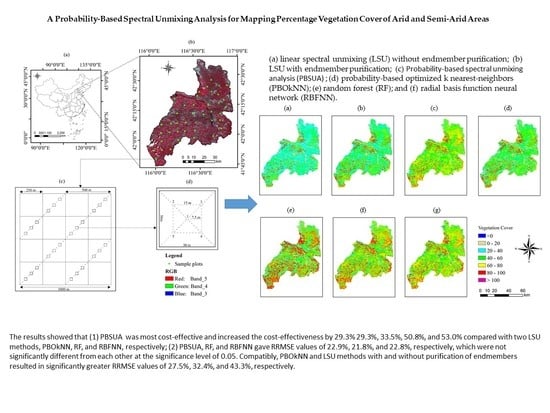
In this study, the overall objective was to develop and evaluate a cost-effective method to map PVC as a significant indicator of land degradation and desertification for the north and northwest areas of China. In these areas, collecting field measurements of PVC is difficult and costly because of the area being remote and sparsely populated. We first presented a method that was used to select and purify endmember pixels from Landsat 8 images by removing those containing multiple components. We then proposed and compared two novel probability-based methods to improve the PVC estimation in a selected study area in terms of accuracy and cost-effectiveness. The methods include a probability-based spectral unmixing analysis (PBSUA) and a probability-based optimal kNN (PBOkNN). The methods were also compared with the widely used LSU, RF, and RBFNN approaches to verify the improvement of estimation accuracy and cost-effectiveness of the proposed methods.

2. Materials and Methods

2.1. Study Area

The study was conducted in Duolun County, located in the southeast of Xilingol League in Inner Mongolia Autonomous Region, China (Figure 1). The county is about 110 km from north to south and 70 km from east to west, with a total area of 3863 km2 and an altitude range of 1150 m to 1800 m. With a continental climate, the study area has an average annual temperature of 1.6 °C and an average annual precipitation of 385 mm. In the study area, the soil types are mainly chestnut soil, aeolian sandy soil, and meadow soil. The area is dominated by grassland, with shrubs and marsh growing in sandy soil. Drought-tolerant herbs and sandy shrubs are the dominant plants. In the 1970s and 1980s, natural disasters combined with land reclamation and overgrazing led to serious soil erosion in Duolun County, which had great influence on the sandstorms of Beijing and Tianjin. To control the sandstorms, the central government initiated a national key ecological construction project that increased the PVC from 0.3 in 2000 to about 0.6 in 2016.

2.2. Data Collection

2.2.1. Remote Sensing Data

The Landsat 8 images acquired on August 8 (Path 123, Row 031) and August 15 (Path 124, Row 031), 2016, were used in the study. The two acquisition dates fell in the time interval of the field survey to be mentioned next. The image from August 8 were of good quality, while clouds were scattered in the southwest corner of the August 15 image. Although the clouds led to poorer quality of the image in this small area, we did not use later images, mainly because in Inner Mongolia Autonomous Region of Northern China, grass starts to wilt and herdsmen start to harvest hay in later August and early September. Using later images could have led to underestimations of PVC. The first 7 bands of the images were used, with a spatial resolution of 30 m × 30 m and a radiometric resolution of 12 bits. The data were level 1T products, in which basic radiometric correction and geometric correction were applied. Choosing the level 1T products instead of Level 2 collection was mainly based on the following considerations. Firstly, the two images were utilized; the August 8 image occupied three-fourths of the study area and had the good quality. The poor quality image from August 15 covered only one-fourth of the area. The clouds affected only 40 plots out of 960 sample plots in the 30 m × 30 m area. Secondly, the radiometric and geometric corrections of Landsat level 2 products were made using the dedicated algorithms developed by the U.S. Geologic Survey. However, the corrections were carried out based on the characteristics of objects, atmospheric conditions, and topographic features across the whole image scene of 185 km × 185 km. However, our study area was only a portion of the scene. The characteristics of the objects, atmospheric conditions, and topographic features from neighboring areas might have influence on the corrections. We would like to conduct the radiometric calibration, atmospheric correction. and precise geometric correction based on the parameters collected locally to reduce the effects from the neighboring regions, and thus to obtain more accurate images than Landsat Level 2 products. Moreover, we used a Trimble GEO 7X global positioning system (GPS) receiver to locate all the 30 m × 30 m sample plots and all the ground control points so that the geometric error of the images had similar characteristics to the position errors of the sample plots.
The radiometric calibration converted the pixel gray values into reflectance values. In order to reduce or eliminate atmospheric influence, the images were corrected using the FLAASH module in ENVI 5.3 and the local parameters collected. After that, the precise geometric correction was carried out using 28 ground control points collected with the Trimble GEO 7X GPS receiver. The Universal Transverse Mercator projection coordinate system was used for registration. The RMSE between the coordinates of the ground control points and the coordinates of the same locations on the corrected image was 0.31 pixels (that is, 9.3 m). After the corrections, the mosaic and clipping processes of the images were further carried out.
We compared the corrected level 1T images using FLAASH with the level 2 products for their quality based on the correlations of NDVI and soil adjusted vegetation index (SAVI) with the PVC from the sample plots. It was found both the level 2 and the locally corrected level 1T products led to the same coefficient of correlation, 0.79, between NDVI and PVC. However, the locally corrected level 1T images resulted in slightly higher correlation of SAVI with PVC than the level 2 images. At the same time, given a vegetation index, the values from the locally corrected level 1T images were highly correlated with those from level 2. In addition, it was found that the level 2 products showed insensitivity for large values of both NDVI and SAVI (the figure was omitted because of the limited space). This implied that the images corrected using FLAASH based on Landsat level 1T products had better quality than those from the level 2 products. Based on the 28 ground control points collected, the level 2 products had a geometric error of 0.30 pixels (that is, 9.0 m). This error was very similar to that (9.3 m) of the level 1T products. The geometric error could ensure almost all five 1 m × 1 m sub-plots systematically allocated in each of the 30 m × 30 m sample plots (Figure 2b) fell in the corresponding pixels when the sample plots were matched with the pixels of the mosaicked image.

2.2.2. Sample Plot Data

A stratified systematic sampling was carried out in Duolun County. Firstly, the NDVI values were extracted from the Landsat 8 mosaic image. The NDVI values were then grouped into five classes with an interval of 0.2. The proportion of each class in the total area was calculated and used to determine the number of sample blocks of each class. Finally, 40 sample blocks of 1000 m × 1000 m were selected from the study area (Figure 1b). To achieve the multiscale and low-cost collection of PVC field observations, the sample sub-blocks of 500 m × 500 m and 250 m × 250 m were designed and nested in each 1000 m × 1000 m sample block (Figure 2a), each containing four 500 m × 500 m sample sub-blocks and sixteen 250 m × 250 m sample sub-blocks. Twelve, six, and three 30 m × 30 m sample plots that had the same spatial resolution of the used images were allocated along the diagonal lines of the 1000 m × 1000 m sample blocks, 500 m × 500 m, and 250 m × 250 m sample sub-blocks, respectively, from the northeast to the southwest. Each 30 m × 30 m sample plot consisted of five 1 m × 1 m sub-plots (Figure 2b). Thus, 160 sample sub-blocks of 500 m × 500 m, 320 sample sub-blocks of 250 m × 250 m, 960 sample plots of 30 m × 30 m, and 4800 sub-plots of 1 m × 1 m were obtained.
The collection of PVC field observations was done between July 13, 2016, and August 20, 2016. The aforementioned Trimble GEO 7X GPS receiver was used to navigate and collect the center coordinates of the 30 m × 30 m sample plots. A compass and a tape were adopted to locate the sub-plots. We recorded the vegetation types and heights and soil types in the sub-plots. Along the west–east and the north–south central lines of the sub-plots, we checked the vegetation cover at an interval of 10 cm, and counted the number of points covered by vegetation. Each PVC value was obtained by dividing the number of the vegetation covered points by the total number of the observed points. The PVC value of each 30 m × 30 m sample plot was the average of the PVC values from five 1 m × 1 m sample sub-plots. In the same way, the PVC values of the 250 m × 250 m and 500 m × 500 m sample sub-blocks and the 1000 m × 1000 m sample blocks were obtained.
Since the mosaicked image used in the study had a spatial resolution of 30 m × 30 m, we only used the field data from the sample plots of 30 m × 30 m. There were 40 sample plots affected by the clouds and removed from the analysis. Finally, there were 920 sample plots of 30 m × 30 m used in the study. Moreover, the sampling design provided the field data from the 1000 m × 1000 m, 500 m × 500 m, and 250 m × 250 m sample sub-blocks, which can be utilized to match the corresponding spatial resolution images from MODIS products to map PVC, although they were not employed in this study. In addition, the PVC values at the spatial resolutions from 30 m × 30 m to 1000 m × 1000 m were not thoroughly measured and were instead obtained by sampling five 1 m × 1 m sample sub-plots, each with two transect lines. Thus, the PVC values should be considered as reference values that were associated with uncertainties.

2.3. Methods

Given an area, the accuracy and cost-effectiveness of estimating PVC using spectral unmixing analysis is, to a great extent, dependent on pure training samples (that is, endmembers) to be selected and the unmixing methods to be used. This is especially true for large areas in which a large number of mixed pixels exist. On the other hand, the measurements of PVC are often obtained by calculating the ratio of the points covered by vegetation canopies to the total number of the points observed in the field, which is then represented by a percentage value. Thus, PVC can be regarded as the probability of vegetation coverage given an area. Moreover, in this study the PVC value of each 30 m × 30 m sample plot was obtained by averaging the PVC values based on the percentages of vegetation-covered points in five 1 m × 1 m sub-plots. This implies a probability of vegetation cover within each of the 30 m × 30 m sample plots. As previously mentioned, the existing linear and nonlinear unmixing methods, including LUS, RF, and BPNN, are not appropriate for mapping PVC for the large and sparsely populated area of northern and northwestern China. A new and applicable method that requires only a few or no field training samples is needed. In this study, we first developed a simple and effective method for selection of endmembers, mainly based on the Landsat 8 image. We then proposed and compared two probability-based spectral unmixing analysis methods.

2.3.1. Selection and Purification of Endmembers

In this study, we examined six endmembers, including woodland, grassland, urbanized area, crop, water, and bare soil. It was found that woodland and grassland had similar spectral reflectance curves, and thus were combined into one endmember (simply called grassland). Finally, five endmembers were determined. Because of a limited cost and a lack of fine spatial resolution images and spectral libraries, in the proposed method the endmembers were directly selected from the 30 m spatial resolution Landsat image. The training pixels of the endmembers were first chosen from the homogeneous areas of the Landsat 8 image by integrating visual interpretation with the NDVI values of the pure sample plots. After substantial experiment and examination based on the field sample plot data, it was found that the NDVI values of pure pixels for water, urbanized area, bare soil, crop, and grassland were −0.8 to −0.5, 0 to −0.1, 0 to −0.05, 0.85 to 1.0, and 0.85 to 1.0, respectively. The 30 m spatial resolution might have led to some impure training pixels that could be regarded as outliers. The one standard deviation-based method of average spectral distance was utilized to remove the outliers. The average spectral distance, d, between any two selected pixels in the same endmember was calculated using the square Euclidean distance:
d = i = 1 m ( x i y i ) 2
where m represents the number of the bands used from the image, and x i , y i are the reflectance values of the ith band for two pixels, respectively. The standard deviation of the average spectral distance in the same endmember was calculated and used to eliminate the impure pixels according to the principle of one standard deviation. The endmember purification was conducted for all five endmembers. This method minimizes the variability of pixel spectral reflectance values within each of the endmembers and purifies the endmembers. The spatial resolution of the used image matches the size of the sample plots used in this study and is close to the plot size utilized in the Chinese national forest inventories. Thus, the proposed method is applicable for mapping PVC in the northern and northwestern China.

2.3.2. Probability-based Spectral Unmixing Analysis (PBSUA)

A spectral center of each endmember was first defined as the average of the reflectance values of all pure pixels for each band after purification in the same endmember. The spectral distance between each mixed pixel and the center of each endmember was calculated. The reciprocal of the spectral distance between the mixed pixel and the spectral center of the endmember was calculated as follows:
w i = 1 d i
where d i represents the spectral distance from the mixed pixel to the spectral center of the ith endmember. The reciprocal of the spectral distance implied the similarity of the mixed pixel to the endmember and was used as the weight of the mixed pixel. The probability of the mixed pixel belonging to the ith endmember was calculated as follows:
p i = w i j = 1 q w j
where p i represents the probability that the mixed pixel belongs to the ith endmember and q is the number of the endmembers. The PVC value of the mixed pixel was derived using the summation of the probabilities of grassland and crop land within the mixed pixel. In the PBSUA, it was assumed that the probability of vegetation cover within a mixed pixel is proportional to the spectral similarity of the mixed pixel to the vegetation endmember.

2.3.3. Probability-based Optimized k-Nearest Neighbors (PBOkNN)

The PBOkNN method is similar to PBSUA for endmember purification, weight, and probability calculation. However, the difference was that given N pure pixels or training samples of all the endmembers, the spectral distance of a mixed pixel to each pure pixel within each of the endmembers was calculated and ranked from the smallest to largest distance. Moreover, an optimal k value was then determined and used to select the k nearest pure pixels. The weight of the mixed pixels within the ith endmember was derived:
w i = k i j = 1 k d i j
In order to derive the optimal k value, two-thirds of the 920 sample plots—that is, 613 plots—were randomly selected and were used. For each sample plot, its PVC value was estimated based on the method mentioned above using all the pure pixels, meaning that k ranged from 1 to the number of the pure pixels. For each k, the RMSE of the PVC was calculated based on the estimated and referenced PVC values of the sample plots. The k value with the smallest RMSE was regarded as optimal.

2.4. Model Performance Assessment

We first compared the results from LSU with and without purification of endmembers to find out whether the purification could improve the estimation of PVC in this study (Table 1). After this, the purified endmembers were used to compare the proposed PBSUA and PBOkNN with the widely used nonlinear methods RF [34,35,36] and RBFNN [33]. Moreover, we used the first seven bands of the image as independent variables and the measured PVC as the dependent variable, which were input into the RF and RBFNN to train the models.
The 920 sample plots in Duolun County were randomly divided into two parts: 613 as the training data and 307 as the test data (Table 1). The PVC estimates obtained by two LSU methods with and without purification of endmembers, PBSUA, PBOkNN, RF, and RBFNN were compared with the field measurements in terms of mean PVC prediction (MPVC), coefficient of determination (R2), RMSE, relative RMSE (RRMSE), relative bias of the test plot data, and coefficient of variation (Covr) of the predicted maps [43,45]. All the methods used the same test dataset to assess their estimation accuracy, but the training datasets varied depending on the methods due to different requirements of data (Table 1). To train the LSU without purification of endmembers, all the pixels selected from the Landsat 8 image before the purification were used. To train both the LSU with purification of endmembers and PBSUA, the pure pixels obtained after the endmember purification were utilized. The same dataset from 613 training sample plots was employed to train both RF and RBFNN models. To training the PBOkNN model, both the pure pixels and 613 training sample plots were utilized. Finally, the cost-effectiveness for each of the methods was assessed. The RRMSE and cost-effectiveness were calculated based on following equations:
R R M S E = i = 1 N ( x ^ i x i ) 2 N x ¯ × 100 %
  C o s t _ e f f e c t i v e n e s s = 1 / ( c o s t   ×   R R M S E )
where N is the number of the test sample plots, x i is the field measurement of the ith plot, x ^ i is the estimated value of the ith plot, and x ¯ is the average of the plot field measurements. In Equation (6), the cost includes the budget used for collection of the field sample plot data and data analysis, and the RRMSE is represented using fraction. The cost-effectiveness for each of the methods was calculated based on the cost required to collect the field data and conduct the data analysis in Table 1. The larger the reciprocal value, the higher the cost-effectiveness.

3. Results

3.1. Statistics of Sample Plot Data

The sample mean values of PVC for the whole, training, and test datasets in the study were 61.3%, 61.4%, and 61.2%, with standard deviations of 24.6%, 24.5%, and 24.6%, and coefficients of variation of 40.1%, 39.3%, and 40.3%, respectively. The sample mean values were not significantly different from each other at the significance level of 0.05, indicating that the division of the whole dataset into the training and validation datasets was reasonable. Based on the sample means and the corresponding standard deviations, the obtained confidence intervals for the whole, training, and test datasets were 59.8%–63.0%, 59.5%–63.4%, and 58.6%–64.1%, respectively.

3.2. Endmember Purification

The spectral characteristic analysis on the endmembers showed that woodland and grassland were almost identical (Figure 3), and thus these two endmembers were merged into one, which finally led to five endmembers. Moreover, several widely used vegetation indices, including NDVI [1,11,19,53], enhanced vegetation index (EVI) [11], SAVI [5], and modified SAVI [5], were used to examine the possibility of separating the woodland from the grassland, but similar results were obtained. The main reason was because there was only a small area located in the southeast part of the study site that was dominated by trees, while most trees were scattered across the study area and mixed with grass. Sequentially, all the analyses were conducted using five endmembers. A total of 10,413 pixels were selected for the five endmembers. The endmember purification removed a total of 1180 pixels, leaving 9233 pixels left, regarded as purified pixels (Table 2). Compared with other endmembers, a smaller number of water pixels and a larger number of crop pixels were removed. This was mainly because the water bodies were relatively pure, while the crop lands had greater potential for plants mixing with soils due to regular planting and sparse canopies.

3.3. Comparison of Methods

In Table 3, the results from all six methods were assessed based on the test plot data. All methods except for two LSU methods led to the PVC average estimates of the test plots and predicted maps falling in the confidence interval at the significance level of 0.05 (Table 3). Both LSU methods with and without purification of endmembers resulted in serious underestimations with large values of RMSE, RRMSE, and relative bias, and their average estimates were much smaller than the sample mean of the test plot data. Compared with the LSU without purification of endmembers, the LSU with endmember purification significantly increased the estimation accuracy of PVC and decreased the RMSE value of predicted PVC by 25.3% (Table 3). The improvement was statistically significant at the significance level of 0.05 (Table 4), implying that the endmember purification significantly increased the accuracy of PVC predictions.
The PBSUA, PBOkNN, RF, and RBFNN methods produced significantly greater estimation accuracy for PVC predictions than the two LSU methods (Table 3 and Table 4). The relative bias values from the two LSU methods were significantly different from zero, but those from PBSUA, PBOkNN, RF, and RBFNN were not. The RF resulted in the greatest R2 and smallest RRMSE, followed by RBFNN, PBSUA, PBOkNN, and LSU with purification of endmembers. The LSU without purification of endmembers led to the smallest R2 and greatest RRMSE (Table 3). The RMSE values from PBSUA, RF, and RBFNN did not significantly differ from each other, but were significantly smaller than that from PBOkNN (Table 3 and Table 4).
In Figure 4, the residuals of the PVC predictions were graphed against the referenced values. The residuals obtained by two LSU methods with and without purification of endmembers showed a decreasing trend with the increase of the PVC referenced value. This indicated that the LSU methods led to overestimations when the PVC values were small, and underestimations when the PVC values were large (Figure 4a,b). The same problem happened for RF and RBFNN, but was much less noticeable (Figure 4e,f). The residual distributions of PBSUA and PBOkNN were relatively uniform and did not show obvious overestimations or underestimations of PVC (Figure 4c,d).
In Figure 5, the spatial distributions of PVC estimates obtained by all the methods were consistent with the vegetation distribution shown by the false color composite image of Landsat 8 band 5 (red), band 4 (green), and band 3 (blue) in terms of the spatial pattern in Figure 1b. The large PVC predictions were mainly distributed in the southwest and northwest parts of Duolun County and the small PVC predictions mainly in the northern part, implying the development of desertification. The PVC estimates obtained by two LSU with and without purification of endmembers were much smaller than those obtained by other methods. The PBSUA, PBOkNN, RF, and RBFNN methods led to more similar and reasonable spatial distributions in terms of both the spatial pattern and value. The clouds in the southwest part of the Landsat 8 image affected the accuracy of PVC estimation in this area.

4. Discussion

4.1. Method for Obtaining Endmembers

The estimation accuracy of spectral unmixing analysis varies, to a great extent, depending on the selection and purification of training samples (endmembers) [19,24,25]. Endmembers are often selected from a library of spectral reflectance, field or laboratory measurements, or fine spatial resolution images. For example, Li et al. [19] selected two endmembers: bare soil and vegetation based on 30 m × 30 m spatial resolution Landsat 8 images and in situ measurements of spectral reflectance and obtained a determination coefficient of 0.54 and a RMSE of 0.17 for estimating fraction of vegetation cover for Inner Mongolia using an improved pixel dichotomy model. This method is simple and easy to apply, but requires endmember field measurements of spectral reflectance. This will greatly increase the cost when it is applied to large areas. Moreover, Roberts et al. [24] proposed a variable endmember spectral unmixing analysis. Dennison and Roberts [25] improved the variable endmember method and obtained a classification accuracy of 88.6% to map six land cover types in the Santa Ynez Mountains using an airborne image. However, the method uses libraries of spectral reflectance for endmembers and is not applicable to mapping PVC for the northern and northwestern China because of the lack of spectral libraries.
There are no general rules that can be used to optimize the selection and purification of endmembers from remote sensing images. In this study, we developed a general method for selection and purification of endmembers using Landsat 8 images at the spatial resolution of 30 m × 30 m to map PVC for large areas. Generally, the 30 m spatial resolution is too coarse to select pure pixels. In this study, the disadvantage was overcome by integrating visual interpretation, use of NDVI values, and purification of endmember pixels. The potentially impure pixels were, thus, removed. It was found that the endmember purification significantly improved the estimation accuracy of PVC in the study area by 25.2%. This was mainly because this method greatly reduced the heterogeneity of the endmember pixels and minimized their reflectance variation within each of the endmembers. Integrating the endmember selection method with the proposed method PBSUA led to coefficient of determination values of 0.679 and RRMSE of 22.9%, indicating significant RRMSE decreases of 47.4% and 29.3% compared with those from the LSU methods without and with the purification of the endmembers, respectively. The PBSUA provided an accuracy value similar to those from RF and RBFNN, but the former was much more cost-effective (discussed next). The results are also compatible with the findings from previous studies [19,24,25]. However, the proposed method for selection of endmembers does not require libraries and field measurements of endmember spectral reflectance, and will greatly reduce the cost of collecting the field observations of spectral reflectance. This is especially important for mapping PVC at regional, national, and global scales.
Theoretically, the proposed method integrates visual-interpretation-based image stratification, spectral-reflectance-based vegetation indices, and statistically an outlier removal method to select and purify the endmember pixels. The pixels that are selected by visual interpretation contain multiple endmembers, and are treated as outliers and removed using vegetation indices and statistical methods. This study showed that although the used Landsat images had a 30 m × 30 m spatial resolution, the images could be successfully utilized to select the endmembers with the proposed method. This implied that the disadvantage of the medium spatial resolution images for selecting endmembers could be compensated by using vegetation indices and statistical methods. Thus, this method overcame a gap that currently exists in the use of medium resolution images to select endmembers and advanced the literature in the field. This method is easier and more promising for application to the selection of endmembers for mapping PVC for large areas than the existing methods. This method also provides the potential to use coarser spatial resolution images such as MODIS products to select endmembers and map PVC at national and global scales.

4.2. Method Comparison by Estimation Accuracy

The multiple scattering often leads to a nonlinear relationship of endmember component fractions with the reflectance values within mixed pixels. The LSU methods lack the ability to model the nonlinear relationship because of their assumption that the spectral reflectance value of a mixed pixel is a convex linear combination of the endmember spectra. Thus, the LSU methods do not work well when the assumption is broken down or landscapes are complex, such as urbanized lands, mountainous areas, and sparsely vegetated areas [20,37,38,39,53,54,55].
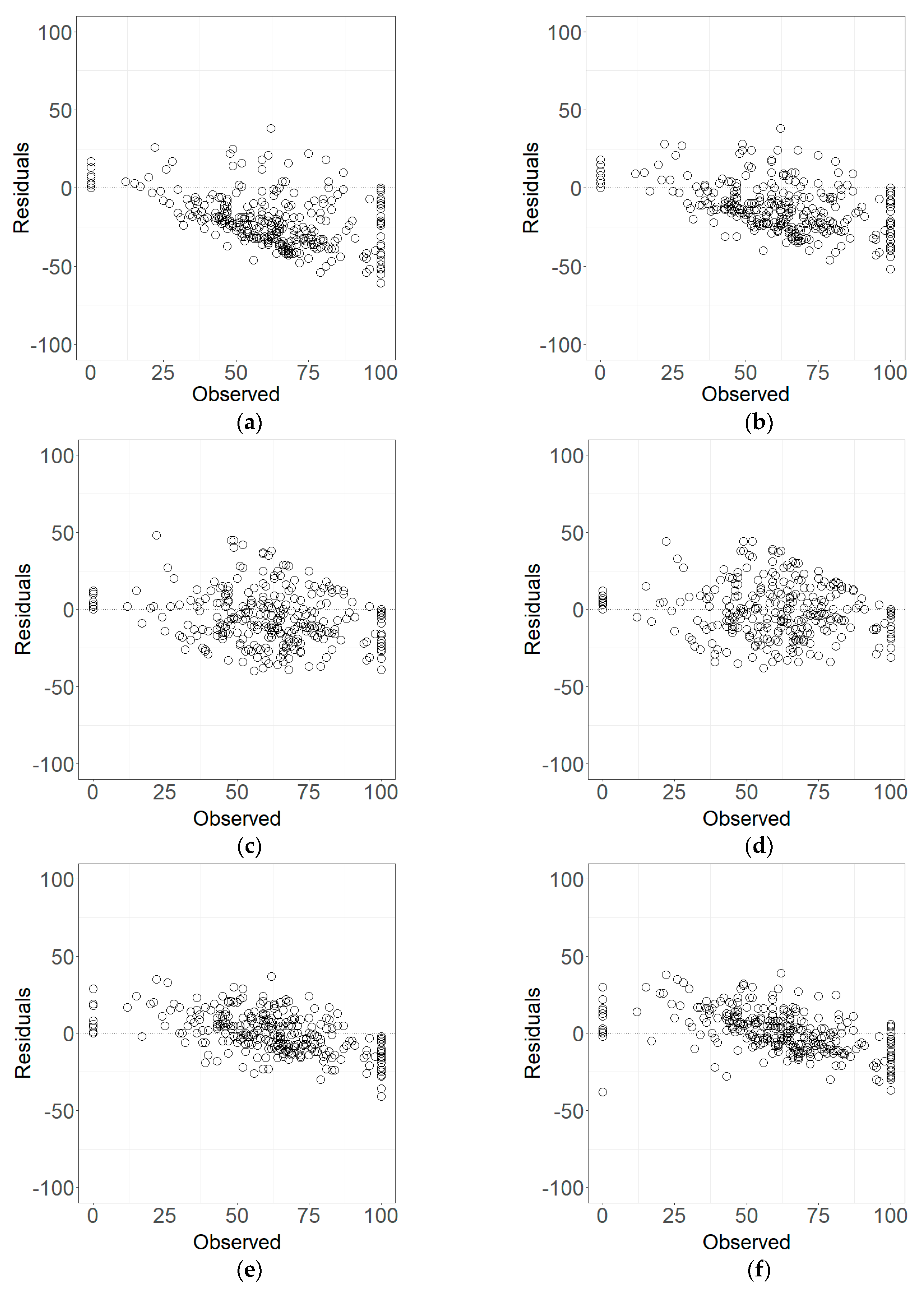
The results of this study showed that compared with two LSU methods with and without the endmember purification, the proposed methods PBSUA and PBOkNN, along with two widely used nonlinear models RF and RBFNN, significantly decreased the RRMSE of PVC estimates (Table 3). The decrease of RRMSE was represented using the difference of RRMSE values between two methods divided by the RRMSE from the compared method. Compared with LSU without the endmember purification, the PBSUA, PBOkNN, RF, and RBFNN methods decreased the RRMSE by 47.1%, 36.5%, 49.7%, and 47.3%, respectively. Compared with LSU with the endmember purification, the PBSUA, PBOkNN, RF, and RBFNN decreased the RRMSE by 29.3%, 15.1%, 32.8%, and 29.7%, respectively. This finding is consistent with the conclusions from previous studies [20,53,54,55]. Yu et al. [54] used Landsat data and compared six linear and nonlinear unmixing methods, including LSU, support vector machine, ANN, and others to estimate fractions of water, forest, and bare land for an area located in Guangxi in China. The authors concluded that all the nonlinear methods decreased the RMSE values by 17.8% to 57.9% compared with the linear approaches. Mitraka et al. [55] used an ANN trained with nonlinear and linear methods, respectively, and concluded that compared with the linear method, the nonlinear ANN decreased the RMSE by 20.4%, 0.0%, 37.6%, and 4.1% for the fraction estimations of built-up area, vegetated area, nonurban bare land, and water, respectively. Similarly, Ahmed et al. [20] presented an ANN-based hybrid approach for switching between linear and nonlinear spectral unmixing of hyperspectral data and found that the hybrid method increased the estimation accuracy of twenty-one endmember fractions by 63.0% to 84.8% compared with the linear and nonlinear models alone. This indicated that the hybrid approach was promising. However, their study used the controlled synthetic data, which covered a small area. Thus, further validation based on real datasets from large and complex landscapes is needed.
Compatibly, machine learning, and nonlinear spectral unmixing methods, especially RF and ANN, are more sensitive to modeling the nonlinear relationship in mixed pixels and have greater potential to provide more accurate estimates of endmember fractions within mixed pixels [20,39,53,54,55]. The nonlinear methods often uses hyperspectral images rather than cheaper multispectral images [37,38,39]. So far, RF has been widely used for image classification, and there have been almost no reports for its application for mapping PVC. Maxwell et al. [56] compared six machine learning classifiers to classify alfalfa, corn, soybeans, wheat, hay, grass, oats, and trees using an airborne visible/infrared imaging spectrometer (AVIRIS) image in Tippecanoe County, Indiana. The classifiers included support vector machines, decision trees, RF,-boosted decision trees, ANN, and kNN. The authors obtained overall classification accuracies of 89.1%, 78.3%, 87.1%, 87.2%, 85.1%, and 78.6%, respectively. The authors also utilized the six methods with high spatial resolution aerial images to distinguish trees, grass, soil, concrete, asphalt, buildings, cars, pools, and shadows in Deerfield Beach, Florida, and yielded overall accuracies of 76.3%, 68.1%, 81.5%, 76.9%, 67.5%, and 72.4%, respectively. However, both RF and ANN are sensitive to training sample size and characteristics [33,35,56].
The previous studies also imply that when the information of an interest variable such as PVC is extracted using spectral unmixing analysis and remote sensing images, both linear and nonlinear relationships of the interest variable with spectral variables may exist in a landscape [20,37,55]. The relationships may vary on a pixel-by-pixel basis or by sub-region. An interest variable may also be characterized by both spatial dependency and heterogeneity. The challenges for improving the performance of the information extraction are first to accurately identify the relationships and characteristics, and then to develop methods to take into account the relationships and characteristics.
In this study, the proposed PBOkNN is an integration of the probability-based decomposition of endmembers with kNN. The kNN is a simple local interpolation technique and has been widely used in forest parameter estimation and mapping, as well as land use and land cover classification, because of its advantage of using k most-similar neighbors in a multiple feature space [45,57,58,59]. In both the proposed PBSUA and PBOkNN, it is assumed that multiple components within each mixed pixel are characterized by the spectral centers of endmembers. The spectral similarity of the mixed pixel to each of the endmembers is quantified using Euclidean distances of spectral features, and then transformed into the probability of the mixed pixel belonging to each of the endmembers. A constraint is used, specifying that the probability summation for all the endmembers within the mixed pixel equals one. This means that both methods are developed based on spectral clustering of similar pixels and endmembers in a multiple dimensional feature space. Within the mixed pixel, the higher the fraction of the endmember component, the more similar the mixed pixel to the endmember and the greater the probability of the mixed pixel belonging to the endmember. In both methods, there is no assumption of linear or nonlinear relationship of PVC with spectral features to be made. Moreover, both methods also transform spatial dependency and heterogeneity into spectral similarity and dissimilarity in a feature space. Thus, the proposed methods provide solutions for the challenges that currently exist in the area of spectral unmixing analysis.
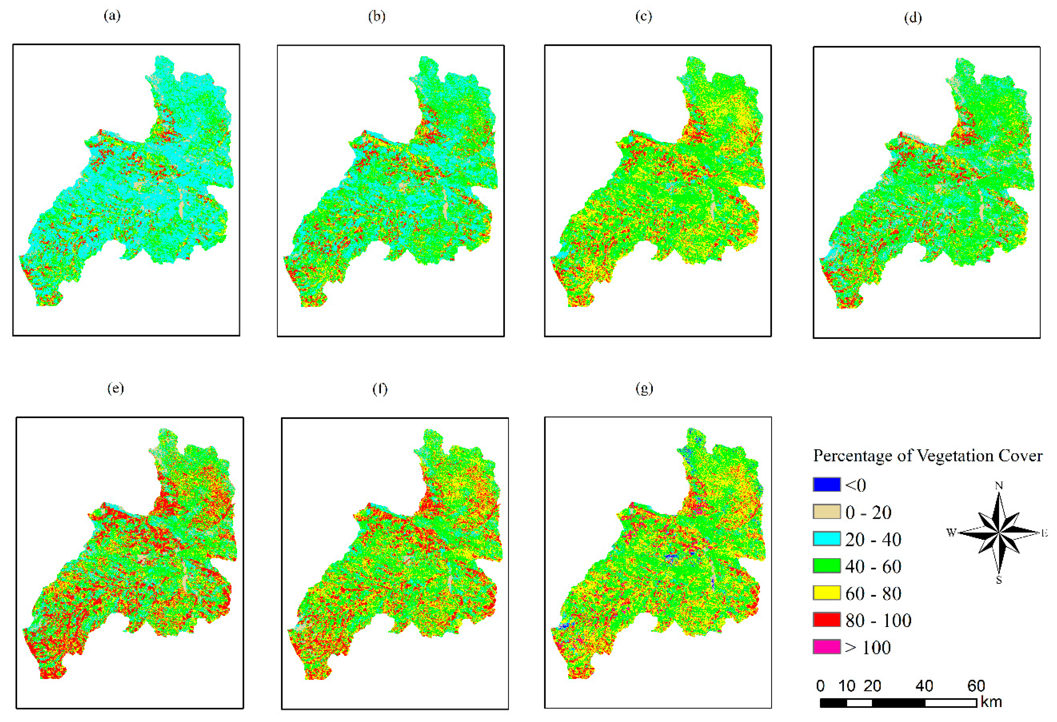
In this study, overall, the PBSUA, PBOkNN, RF, and RBFNN methods had statistically similar accuracies of PVC predictions, indicating that two proposed methods were compatible with the nonlinear unmixing methods. However, the arid and semi-arid areas are sparsely populated and it is often difficult to collect sample field data. Thus, given an estimation accuracy required, the fewer sample plots a method needs, the better the model. Because the pure pixels of the endmembers were selected from the Landsat image, the proposed PBSUA did not need the field plot data for training, except for the test plots. Both RF and RBFNN required a large number of field sample plots for training in addition to the test plots. Similarly, the proposed PBOkNN also needed the field sample plots to determine the optimized k value in addition to the test plots. Additionally, RBFNN produced the PVC estimates less than 0.0% and greater than 100%, which were not reasonable. This implies that the proposed PBSUA has a more significant advantage in terms of accuracy, reasonable predictions, and cost, and is especially appropriate for mapping PVC for large and sparsely populated areas.
The proposed PBOkNN is similar to PBSUA in terms of selection of endmembers and model training. However, it is still unknown how many sample plots are sufficient to determine the optimal k value for PBOkNN. In order to account for the influence of the sample sizes on the estimation accuracy of PVC using this method, we randomly selected and compared four datasets from the field sample plots to map PVC. The datasets consisted of one-fifth (123 plots), two-fifths (245 plots), three-fifths (368 plots), and four-fifths (490 plots) of the field sample plots. The validation results showed that the average values of the estimates varied from 59.6% to 60.2%, all falling within the confidence interval of the test sample data. The RRMSE values slightly decreased from 28.0% to 27.5%. That is, the estimation accuracies of PVC by the different numbers of the sample plots were not statistically significantly different from each other, implying that the sample sizes did not have a great impact on the estimation accuracy of PVC using PBOkNN. The results of this method became stable and achieved the desired accuracy with 123 training plots. The main reason might be because the k nearest plots at each location were selected based on the smallest RMSE between the estimated and referenced PVC values, and the sample size of 123 training plots was large enough to result in stable estimates. On the other hand, when the number of the sample plots was larger than the required number, the plot data tended to be similar to each other. This implied that once the sample plot data is enough, adding more sample plots would not significantly increase the estimation accuracy. This characteristic of PBOkNN provides the potential to reduce the cost for collection of field plot data, which is favorable for mapping PVC for large areas.
The main objective of this study is to develop a cost-effective method for mapping PVC towards a generalized framework of monitoring the dynamics of vegetation cover for large and sparsely populated arid and semi-arid areas in northern and northwestern China. In this study, we used two Landsat 8 images that had a spatial resolution of 30 m × 30 m and a temporal resolution of 16 days. The advantage of the proposed PBSUA and PBOkNN is that the collection of field data for endmembers to train the model can be greatly reduced or avoided. Moreover, the 16-day temporal resolution of Landsat 8 imagery is relatively too coarse to achieve the near real-time monitoring of PVC in the investigated areas. An alternative is using MODIS products that have finer temporal resolutions. For example, Anees and Aryal [60] developed a near real-time detection framework for occurrence of beetle infestation in pine forests using the time series of eight-day 500 m spatial resolution MODIS data collected over five years. In this framework, each of seven vegetation indices was fit by an underlying triply modulated cosine model to derive a stationary vegetation index time series. Based on standard martingale central limit theorem and Gaussian distribution, any non-stationarity in the time series could be detected, indicating beetle infestations. Anees et al. [61] further improved this method so that it could be applied to non-Gaussian time series data to detect near real-time land cover changes using a MODIS NDVI time series. The previous studies imply that the integration of the two proposed methods—especially PBSUA—and the detection framework from Anees and Aryal [60] would make it possible to develop a near real-time monitoring approach for PVC dynamics for large arid and semi-arid areas. In the integration, PBSUA can be used to select endmember pixels from Landsat images, and the monitoring framework of PVC changes can then be generated by combining PBSUA and the method of Anees and Aryal [60] based on the times series of vegetation cover probability from MODIS products.

4.3. Method Comparison by Cost-Effectiveness

Substantial research has been conducted to compare classification accuracies of various linear and nonlinear unmixing methods using remote sensing imagery, but there have been almost no reports that deal with direct comparison of cost-effectiveness among the methods. However, the cost-effectiveness analysis becomes very important for mapping PVC for large areas, because some of the methods are sensitive to the training sample size and computation time, while others not. This will lead to different cost-efficiencies. In the studies related to mapping soil erosion induced by vegetation cover disturbance, Anderson et al. [62] and Wang et al. [63] defined the per sample unit cost-effectiveness as the product of sampling cost per sample unit and average relative error. The authors found that the cost-effectiveness of local variability-based sampling was 5% to 40% higher than that of random sampling. The reason was mainly because the former resulted in the optimized sampling distances and minimized the duplication of information that often takes place in a random sampling design. Wang et al. [64] investigated the cost-effectiveness of the data from different sample plot sizes and image pixel sizes for mapping soil erosion, and concluded that the 20 m spatial resolution sample plot data offered the highest cost-effectiveness of predictions.
In this study, we compared and analyzed the cost-effectiveness of the methods. The analysis did not include the LSU without purification of endmembers because it had almost the same cost as the LSU with purification of endmembers, which had a higher estimation accuracy. The cost of mapping PVC in this study was 150 thousand RMB yuan (1$ = 7.05 yuan), consisting of 120 thousand yuan for the collection of the field data and 30 thousand yuan for the data processing and analysis. The LSU with purification of endmembers and the proposed PBSUA used 307 sample plots as the test data, implying a cost of 40 thousand yuan. The proposed PBOkNN, RF, and RBFNN used all the sample plots, and the total cost was 150 thousand yuan. Thus, the cost-efficiencies of LSU with purification of endmembers, PBSUA, PBOkNN, RF, and RBFNN were 0.0441, 0.0624, 0.0243, 0.0307, and 0.0293, respectively. This indicated that the proposed PBSUA was most cost-effective, followed by LSU with purification of endmembers, RF, RBFNN, and PBOkNN. The PBOkNN had a cost-effectiveness of 0.0243 when a total of 613 sample plots were used to determine the optimal k value. In this method, however, when the number of the sample plots used to determine the optimal k value varied from 613 to 490, 368, 245, and 123, its estimation accuracy changed very slightly, while its cost-effectiveness increased from 0.0243 to 0.0266, 0.0302, 0.0350, and 0.0415, respectively. This implied that when a total of 123 sample plots were used, PBOkNN achieved a higher cost-effectiveness than RF and RBFNN.
Due to the difficulty and high cost of collecting field data in the arid and semi-arid areas, the methods with higher cost-effectiveness should provide greater potential for improving PVC estimation. In this study, RF and RBFNN had higher PVC estimation accuracy, but both used a total of 613 sample plots to train the models. The proposed PBOkNN also needed at least 123 sample plots to determine the optimal k value. The use of the training sample plots lowered the cost-effectiveness of RF, RBFNN, and PBOkNN, and thus they were not appropriate for applications to map PVC for large and sparsely populated arid and semi-arid areas. Because of only using the pure pixels from the Landsat 8 image as the endmembers and the fact that field sample plot data was not needed, the LSU with purification of endmembers had a cost-effectiveness higher than that of other methods, except for PBSUA. However, the LSU with purification of endmembers led to average estimates of the sample plots and the prediction map that were out of the confidence interval of the test dataset, and thus should not be selected for mapping. Moreover, the proposed PBSUA also did not need field sample plot data, but resulted in estimation accuracy that was only slightly lower than those from RF and RBFNN. Thus, PBSUA had the highest cost-effectiveness, implying the best performance for mapping PVC in this study. It is expected that this method can be applied to map PVC for the whole arid and semi-arid area of northern and northwestern China.

4.4. Method Application

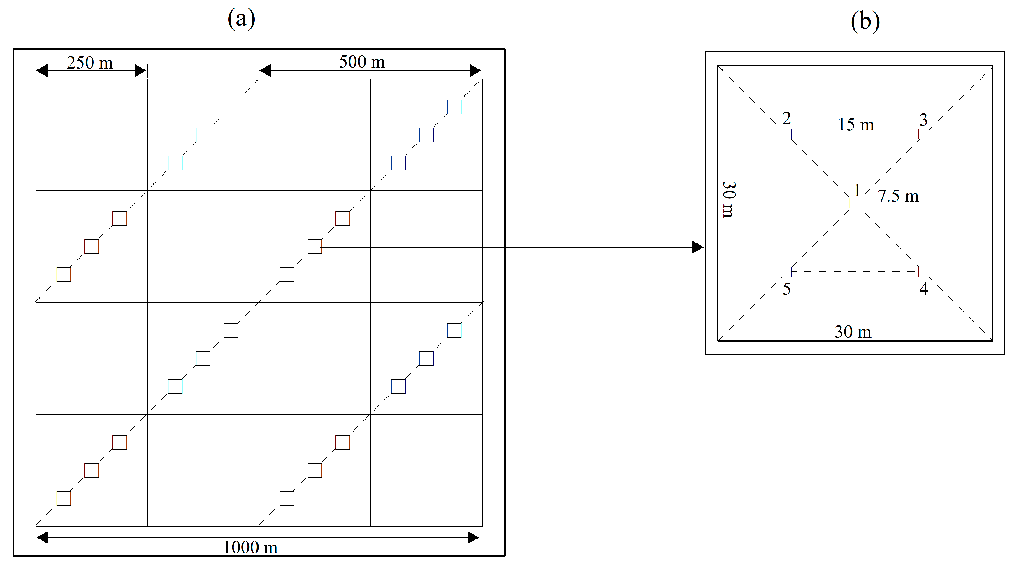
This study is part of a large research project that deals with development and evaluation of cost-effective methods used to map PVC for north and northwest China. In this area, monitoring land degradation and desertification expansion is needed, but collecting field measurements of PVC is difficult and costly because of the area being remote and sparsely populated. In this study, Duolun county is selected because of its representativeness in terms of topography, soil, and vegetation. In addition, there is a need for monitoring the dynamics of PVC and examining the effect of the national key ecological construction project starting in this county in 2000. The size of this study area is relatively small, but it is acceptable because this study focuses on the development and evaluation of the proposed methods, with a large sample size of 920 sample plots of 30 m × 30 m. In the future study, it is expected that the most cost-effective method should be further assessed in larger areas.
The results showed that the proposed PBSUA method is the most cost-effective for mapping PVC in Duolun county using the Landsat 8 imagery. This method is simple and consists of selecting endmembers, deriving spectral similarity of mixed pixels to each endmember and estimating the probability of each mixed pixel belonging to each endmember. In this method, one standard deviation of the average spectral distance among the selected pixels within the same endmember is utilized to remove the impure pixels. The probability of vegetation cover within a mixed pixel is then estimated based on the spectral similarities of the mixed pixel to the vegetation endmembers. The PVC value of the mixed pixel is finally obtained by summing the probabilities of relevant vegetation cover components, including grassland and crop land in this study. In fact, the grassland area actually consists of grassland and woodland in this study. In future studies, the grassland and woodland areas could be separated and other vegetation relevant components could be added. In addition, this method is generalized and can be applied to any study of spectral unmixing analysis using spectral variables from remote sensing data, such as Sentinel-2 and SPOT imagery.
In this study, we only used the original bands of the Landsat 8 image instead of various vegetation indices. This was mainly because of the following reasons: (1) This study focused on the development of the proposed PBSUA and its comparison with other wisely used methods. Thus, using the same set of spectral variables simplified and standardized the assessment of cost-effectiveness among the methods. (2) Because different methods may be sensitive to different spectral variables, such as vegetation indices, using different spectral variables for the methods would impede the consistent assessment of cost-effectiveness. (3) Using the original bands calibrated the method assessment of cost-effectiveness and did not affect the generalization of applications for the proposed PBSUA. In the future studies, the proposed method can be further evaluated using various vegetation indices.
It has to be pointed out that compared with finer spatial resolution images, such as those from Sentinel 2, using the 30 m × 30 m resolution Landsat images in this study increased the number of mixed pixels. This method is, thus, prone to estimation errors of PVC due to the mixed pixels. On the other hand, using 10 m × 10 m spatial resolution Sentinel 2 images would reduce the number of mixed pixels, and thus the estimation error of PVC due to mixed pixels. Compared with Landsat images, however, using Sentinel 2 images would result in a nine-fold increase of data and computation intensity. This indicates a trade-off. China has a desertification land area of about 4,354,800 km2. Annually providing the decision-makers with information related to land desertification dynamics at the national scale is necessary. Because of the large area, limited budget, and requirement for fast acquisition and analysis of data, developing a cost-effective method to map PVC for the whole desertification area of China is critical. Various spatial resolution satellite images should be analyzed for their cost-effectiveness. This study could be regarded as a pilot study for a larger research project. In the future, a comparison of the uses of Landsat and Sentinel images in terms of accuracy and cost-effectiveness is needed.

5. Conclusions

To develop a cost-effective method to map PVC in the north and northwest arid and semi-arid area of China, a Landsat image-based endmember selection approach was first presented. Then, two probability-based spectral unmixing methods, PBSUA and PBOkNN, were proposed and compared with two LSU methods, with and without purification of endmembers, and two nonlinear methods, RF and RBFNN. The comparisons were conducted to improve the estimation accuracy of PVC in terms of mapping accuracy and cost-effectiveness in Duolun County, located in Inner Mongolia Autonomous Region, China, using Landsat 8 images and 920 sample plots. The study led to the following conclusions: (1) the proposed PBSUA was most cost-effective, followed by the two LSU methods, PBOkNN, RF, and RBFNN, but the two LSU methods led to significant underestimations; (2) the accuracy of mapping PVC using PBSUA was only slightly lower than those using RF and RBFNN, but significantly higher than that using PBOkNN; (3) the PBSUA, PBOkNN, RF, and RBFNN methods resulted in significantly higher estimation accuracies than two LSU methods; (4) the PBSUA, PBOkNN, RF, and RBFNN methods produced average estimates of the sample plots and the predicted maps that fell within the confidence interval of the test plot data, but the two LSU methods did not; and (5) the LSU method with purification of endmembers greatly improved the PVC estimation accuracy compared with the LSU method without purification of endmembers. These findings imply that a cost-effective method should be characterized by the capacity to handle both linear and nonlinear relationships of PVC with spectral variables, and spatial dependency and heterogeneity, with the requirement of few or no field samples. Among the compared methods, the proposed PBSUA method possesses these characteristics, and thus is appropriate for cost-effectively mapping PVC for the arid and semi-arid areas of northern and northwestern China.

Author Contributions

All authors have read and agreed to the published version of the manuscript. Conceptualization, H.S. and G.W.; methodology, H.S. and G.W.; validation, C.L.; formal analysis, C.L.; investigation, Y.C., H.S., and X.X.; writing—original draft, Y.C., H.S., and C.L.; supervision, H.S.; writing—review and editing, G.W.; project administration, G.W.; funding acquisition, H.S. All authors have read and agreed to the published version of the manuscript.

Funding

This research was funded by the National Bureau to Combat Desertification, State Forestry Administration of China, grant number101-9899; Scientific Research Fund of Hunan Provincial Education Department, grant number 17A225; the project of the National Key R&D Program of China, grant number 2017YFC0506502 and Training Fund of Young Professors from Hunan Provincial Education Department, grant number 90102-7070220090001.

Conflicts of Interest

The authors declare no conflict of interest.

References

  1. Eckert, S.; Hüsler, F.; Liniger, H.; Hodel, E. Trend analysis of MODIS NDVI time series for detecting land degradation and regeneration in Mongolia. J. Arid Environ. 2015, 113, 16–28. [Google Scholar] [CrossRef]
  2. Liu, F.; Chen, Y.; Lu, H.; Shao, H. Albedo indicating land degradation around the Badain Jaran Desert for better land resources utilization. Sci. Total Environ. 2016, 578, 67–73. [Google Scholar] [CrossRef] [PubMed]
  3. Li, J.; Liu, Z.; He, C.; Tu, W.; Sun, Z. Are the drylands in northern China sustainable? A perspective from ecological footprint dynamics from 1990 to 2010. Sci. Total Environ. 2016, 553, 223–231. [Google Scholar] [CrossRef] [PubMed]
  4. Lamchin, M.; Lee, J.-Y.; Lee, W.-K.; Lee, E.J.; Kim, M.; Lim, C.-H.; Choi, H.A.; Kim, S.-R. Assessment of land cover change and desertification using remote sensing technology in a local region of Mongolia. Adv. Space Res. 2016, 57, 64–77. [Google Scholar] [CrossRef]
  5. Zhang, X.; Liao, C.; Li, J.; Sun, Q. Fractional vegetation cover estimation in arid and semi-arid environments using HJ-1 satellite hyperspectral data. Int. J. Appl. Earth Obs. Geoinf. 2013, 21, 506–512. [Google Scholar] [CrossRef]
  6. Ray, T.W.; Murray, B.C. Nonlinear spectral mixing in desert vegetation. Remote Sens. Environ. 1996, 55, 59–64. [Google Scholar] [CrossRef]
  7. Arneth, A. CLIMATE SCIENCE Uncertain future for vegetation cover. Nature 2015, 524, 44–45. [Google Scholar] [CrossRef] [Green Version]
  8. Wei, X.; Li, Q.; Zhang, M.; Giles-Hansen, K.; Liu, W.; Fan, H.; Wang, Y.; Zhou, G.; Piao, S.; Liu, S. Vegetation cover-another dominant factor in determining global water resources in forested regions. Glob. Chang. Biol. 2017, 24, 786–795. [Google Scholar] [CrossRef]
  9. Coy, A.; Rankine, D.; Taylor, M.; Nielsen, D.; Cohen, J. Increasing the Accuracy and Automation of Fractional Vegetation Cover Estimation from Digital Photographs. Remote Sens. 2016, 8, 474. [Google Scholar] [CrossRef] [Green Version]
  10. Zhou, G.; Liu, S. Estimating ground fractional vegetation cover using the double-exposure method. Int. J. Remote Sens. 2015, 36, 6085–6100. [Google Scholar] [CrossRef]
  11. Jia, K.; Liang, S.; Gu, X.; Baret, F.; Wei, X.; Wang, X.; Yao, Y.; Yang, L.; Li, Y. Fractional vegetation cover estimation algorithm for Chinese GF-1 wide field view data. Remote Sens. Environ. 2016, 177, 184–191. [Google Scholar] [CrossRef]
  12. Gutman, G.; Ignatov, A. The derivation of the green vegetation fraction from NOAA_AVHRR data for use in numerical weather prediction models. Int. J. Remote Sens. 1998, 19, 1533–1543. [Google Scholar] [CrossRef]
  13. Jia, K.; Liang, S.; Liu, S.; Li, Y.; Xiao, Z.; Yao, Y.; Jiang, B.; Zhao, X.; Wang, X.; Xu, S.; et al. Global Land Surface Fractional Vegetation Cover Estimation Using General Regression Neural Networks from MODIS Surface Reflectance. IEEE Trans. Geosci. Remote Sens. 2015, 53, 4787–4796. [Google Scholar] [CrossRef]
  14. Lu, Y.; Coops, N.C.; Hermosilla, T. Estimating urban vegetation fraction across 25 cities in pan-Pacific using Landsat time series data. ISPRS J. Photogramm. Remote Sens. 2017, 126, 11–23. [Google Scholar] [CrossRef]
  15. Hassan, S.M.; Soliman, O.S.; Mahmoud, A.S. Optimized Data Input for the Support Vector Machine Classifier Using Aster Data. Case Study: Wadi Atalla Area, Eastern Desert. Egypt Carpathian J. Earth Environ. Sci. 2015, 10, 15–26. [Google Scholar]
  16. Sun, H.; Wang, Q.; Wang, G.; Lin, H.; Luo, P.; Li, J.; Zeng, S.; Xu, X.; Ren, L. Optimizing kNN for Mapping Vegetation Cover of Arid and Semi-Arid Areas Using Landsat images. Remote Sens. 2018, 10, 1248. [Google Scholar] [CrossRef] [Green Version]
  17. Lin, M.L.; Chu, C.M.; Shih, J.Y.; Wang, Q.B.; Chen, C.W.; Wang, S.; Tao, Y.H.; Lee, Y.T. Assessment and monitoring of desertification using satellite imagery of MODIS in East Asia. Agriculture and Hydrology Applications of Remote Sensing. In Proceedings of the Society of Photo-Optical Instrumentation Engineers (SPIE); Kuligowski, R.J., Parihar, J.S., Saito, G., Eds.; SPIE: Bellingham, WA, USA, 2006; Volume 6411, p. 641123. [Google Scholar]
  18. Liu, Q.; Liu, G.; Huang, C. Monitoring desertification processes in Mongolian Plateau using MODIS tasseled cap transformation and TGSI time series. J. Arid Land 2018, 10, 12–26. [Google Scholar] [CrossRef] [Green Version]
  19. Li, F.; Chen, W.; Zeng, Y.; Zhao, Q.; Wu, F. Improving Estimates of Grassland Fractional Vegetation Cover Based on a Pixel Dichotomy Model: A Case Study in Inner Mongolia, China. Remote Sens. 2014, 6, 4705–4722. [Google Scholar] [CrossRef] [Green Version]
  20. Ahmed, A.; Duran, O.; Zweiri, Y.; Smith, M. Hybrid Spectral Unmixing: Using Artificial Neural Networks for Linear/Non-Linear Switching. Remote Sens. 2017, 9, 775. [Google Scholar] [CrossRef] [Green Version]
  21. Shi, C.; Wang, L. Incorporating spatial information in spectral unmixing: A review. Remote Sens. Environ. 2014, 149, 70–87. [Google Scholar] [CrossRef]
  22. Sun, D. Detection of dryland degradation using Landsat spectral unmixing remote sensing with syndrome concept in Minqin County, China. Int. J. Appl. Earth Obs. Geoinf. 2015, 41, 34–45. [Google Scholar] [CrossRef]
  23. Heylen, R.; Parente, M.; Gader, P. A Review of Nonlinear Hyperspectral Unmixing Methods. IEEE J. Sel. Top. Appl. Earth Obs. Remote Sens. 2014, 7, 1844–1868. [Google Scholar] [CrossRef]
  24. Roberts, D.A.; Gardner, M.; Church, R.; Ustin, S.; Scheer, G.; Green, R.O. Mapping chaparral in the Santa Monica Mountains using multiple endmember spectral mixture models. Remote Sens. Environ. 1998, 65, 267–279. [Google Scholar] [CrossRef]
  25. Dennison, P.E.; Roberts, D.A. Endmember selection for multiple endmember spectral mixture analysis using endmember average RMSE. Remote Sens. Environ. 2003, 87, 123–135. [Google Scholar] [CrossRef]
  26. Meyer, T.; Okin, G.S. Evaluation of spectral unmixing techniques using MODIS in a structurally complex savanna environment for retrieval of green vegetation, nonphotosynthetic vegetation, and soil fractional cover. Remote Sens. Environ. 2015, 161, 122–130. [Google Scholar] [CrossRef]
  27. Zhang, X.; Shang, K.; Cen, Y.; Shuai, T.; Sun, Y. Estimating ecological indicators of karst rocky desertification by linear spectral unmixing method. Int. J. Appl. Earth Obs. Geoinf. 2014, 31, 86–94. [Google Scholar] [CrossRef] [Green Version]
  28. Hapke, B. Bidirectional reflectance spectroscopy: 1. Theory. J. Geophys. Res. Solid Earth 1981, 86, 3039–3054. [Google Scholar] [CrossRef]
  29. Li, J.; Li, X.R.; Huang, B.M.; Zhao, L.Y. Hopfield Neural Network Approach for Supervised Nonlinear Spectral Unmixing. IEEE Geosci. Remote Sens. Lett. 2016, 13, 1002–1006. [Google Scholar] [CrossRef]
  30. Liu, W.; Seto, K.C.; Wu, E.Y.; Gopal, S.; Woodcock, C.E. ART-MMAP: A neural network approach to subpixel classification. IEEE Trans. Geosci. Remote Sens. 2004, 42, 1976–1983. [Google Scholar]
  31. Zhang, L.; Wu, B.; Huang, B.; Li, P. Nonlinear estimation of subpixel proportion via kernel least square regression. Int. J. Remote Sens. 2007, 28, 4157–4172. [Google Scholar] [CrossRef]
  32. Altmann, Y.; Dobigeon, N.; McLaughlin, S.; Tourneret, J.Y. Nonlinear Spectral Unmixing of Hyperspectral Images Using Gaussian Processes. IEEE Trans. Signal Process. 2013, 61, 2442–2453. [Google Scholar] [CrossRef] [Green Version]
  33. Singh, A.; Singh, K.K. Satellite image classification using Genetic Algorithm trained radial basis function neural network, application to the detection of flooded areas. J. Vis. Commun. Image Represent. 2017, 42, 173–182. [Google Scholar] [CrossRef]
  34. Akar, Ö.; Güngör, O. Integrating multiple texture methods and NDVI to the Random Forest classification algorithm to detect tea and hazelnut plantation areas in northeast Turkey. Int. J. Remote Sens. 2015, 36, 442–464. [Google Scholar] [CrossRef]
  35. Belgiu, M.; Drăguţ, L. Random forest in remote sensing: A review of applications and future directions. ISPRS J. Photogramm. Remote Sens. 2016, 114, 24–31. [Google Scholar] [CrossRef]
  36. Hao, P.Y.; Zhan, Y.L.; Wang, L.; Niu, Z.; Shakir, M. Feature Selection of Time Series MODIS Data for Early Crop Classification Using Random Forest: A Case Study in Kansas, USA. Remote Sens. 2015, 7, 5347–5369. [Google Scholar] [CrossRef] [Green Version]
  37. Fevotte, C.; Dobigeon, N. Nonlinear Hyperspectral Unmixing With Robust Nonnegative Matrix Factorization. IEEE Trans. Image Process. 2015, 24, 4810–4819. [Google Scholar] [CrossRef] [Green Version]
  38. Altmann, Y.; Pereyra, M.; McLaughlin, S. Bayesian Nonlinear Hyperspectral Unmixing With Spatial Residual Component Analysis. IEEE Trans. Comput. Imaging 2015, 1, 174–185. [Google Scholar] [CrossRef] [Green Version]
  39. Dobigeon, N.; Tourneret, J.-Y.; Richard, C.; Bermudez, J.C.M.; McLaughlin, S.; Hero, A.O. Nonlinear Unmixing of Hyperspectral Images: Models and Algorithms. IEEE Signal Process. Mag. 2014, 31, 82–94. [Google Scholar] [CrossRef] [Green Version]
  40. McRoberts, R.E.; Nelson, M.D.; Wendt, D.G. Stratified estimation of forest area using satellite imagery, inventory data, and the k-Nearest Neighbors technique. Remote Sens. Environ. 2002, 82, 457–468. [Google Scholar] [CrossRef]
  41. Tomppo, E.; Halme, M. Using coarse scale forest variables as ancillary information and weighting of variables in k-NN estimation: A genetic algorithm approach. Remote Sens. Environ. 2004, 92, 1–20. [Google Scholar] [CrossRef]
  42. Tomppo, E.O.; Gagliano, C.; De Natale, F.; Katila, M.; McRoberts, R.E. Predicting categorical forest variables using an improved k-Nearest Neighbour estimator and Landsat imagery. Remote Sens. Environ. 2009, 113, 500–517. [Google Scholar] [CrossRef]
  43. McRoberts, R.E.; Næsset, E.; Gobakken, T. Optimizing the k-Nearest Neighbors technique for estimating forest aboveground biomass using airborne laser scanning data. Remote Sens. Environ. 2015, 163, 13–22. [Google Scholar] [CrossRef]
  44. McRoberts, R.E.; Magnussen, S.; Tomppo, E.O.; Chirici, G. Parametric, bootstrap, and jackknife variance estimators for the k-Nearest Neighbors technique with illustrations using forest inventory and satellite image data. Remote Sens. Environ. 2011, 115, 3165–3174. [Google Scholar] [CrossRef]
  45. Zhu, J.; Huang, Z.; Sun, H.; Wang, G. Mapping Forest Ecosystem Biomass Density for Xiangjiang River Basin by Combining Plot and Remote Sensing Data and Comparing Spatial Extrapolation Methods. Remote Sens. 2017, 9, 241. [Google Scholar] [CrossRef] [Green Version]
  46. The Report of the Fourth Desertification Land Inventory. 2017. Available online: http://www.china.com.cn/fangtan/zhuanti/2017-09/03/content_41523193.htm (accessed on 22 September 2019).
  47. Bian, Z.; Zhang, K. Evaluation of China’s land desertification: A review. Sci. Soil Water Conserv. 2010, 8, 105–112. [Google Scholar]
  48. Li, Y.; Yang, S.; Zhu, X.; Xu, B. Application development of remote sensing technologies to monitoring land desertification of China. Prog. Geogr. 2009, 28, 55–62. [Google Scholar]
  49. Jiang, M.; Zhang, X.F.; Tong, Q.X. Monitoring and evaluation of desertification in Shihezi area using Landsat TM imagery. In Proceedings of the SPIE-The International Society for Optical Engineering, Chengdu, China, 25–29 May 2009; Volume 7471, p. 10. [Google Scholar]
  50. Lin, M.L.; Chen, C.W.; Wang, Q.B.; Cao, Y.; Shih, J.Y.; Lee, Y.T.; Chen, C.Y.; Wang, S. Fuzzy model-based assessment and monitoring of desertification using MODIS satellite imagery. Eng. Comput. 2009, 26, 745–760. [Google Scholar] [CrossRef]
  51. Albalawi, E.K.; Kumar, L. Using remote sensing technology to detect, model and map desertification: A review. J. Food Agric. Environ. 2013, 11, 791–797. [Google Scholar]
  52. Sternberg, T.; Tsolmon, R.; Middleton, N.; Thomas, D. Tracking desertification on the Mongolian steppe through NDVI and field-survey data. Int. J. Digit. Earth 2011, 4, 50–64. [Google Scholar] [CrossRef]
  53. Heylen, R.; Scheunders, P. A Multilinear Mixing Model for Nonlinear Spectral Unmixing. IEEE Trans. Geosci. Remote Sens. 2016, 54, 240–251. [Google Scholar] [CrossRef]
  54. Yu, J.; Chen, D.; Lin, Y.; Ye, S. Comparison of linear and nonlinear spectral unmixing approaches: A case study with multispectral TM imagery. Int. J. Remote Sens. 2016, 38, 773–795. [Google Scholar] [CrossRef]
  55. Mitraka, Z.; Del Frate, F.; Carbone, F. Nonlinear Spectral Unmixing of Landsat Imagery for Urban Surface Cover Mapping. IEEE J. Sel. Top. Appl. Earth Obs. Remote Sens. 2016, 9, 3340–3350. [Google Scholar] [CrossRef]
  56. Maxwell, A.E.; Warner, T.A.; Fang, F. Implementation of machine-learning classification in remote sensing: An applied review. Int. J. Remote Sens. 2018, 39, 2784–2817. [Google Scholar] [CrossRef] [Green Version]
  57. McRoberts, R.E. Estimating forest attribute parameters for small areas using nearest neighbors techniques. For. Ecol. Manag. 2012, 272, 3–12. [Google Scholar] [CrossRef]
  58. Tan, K.; Hu, J.; Li, J.; Du, P.J. A novel semi-supervised hyperspectral image classification approach based on spatial neighborhood information and classifier combination. ISPRS J. Photogramm. Remote Sens. 2015, 105, 19–29. [Google Scholar] [CrossRef]
  59. Mura, M.; McRoberts, R.E.; Chirici, G.; Marchetti, M. Statistical inference for forest structural diversity indices using airborne laser scanning data and the k-Nearest Neighbors technique. Remote Sens. Environ. 2016, 186, 678–686. [Google Scholar] [CrossRef]
  60. Anees, A.; Aryal, J. A Statistical Framework for Near-Real Time Detection of Beetle Infestation in Pine Forests Using MODIS Data. IEEE Geosci. Remote Sens. Lett. 2014, 11, 1717–1721. [Google Scholar] [CrossRef]
  61. Anees, A.; Aryal, J.; O’Reilly, M.M.; Gale, T.J. A Relative Density Ratio-Based Framework for Detection of Land Cover Changes in MODIS NDVI Time Series. IEEE J. Sel. Top. Appl. Earth Obs. Remote Sens. 2016, 9, 3359–3370. [Google Scholar] [CrossRef]
  62. Anderson, A.B.; Wang, G.; Gertner, G.Z. Local variability based sampling for mapping a soil erosion cover factor by co-simulation with Landsat TM images. Int. J. Remote Sens. 2006, 27, 2423–2447. [Google Scholar] [CrossRef]
  63. Wang, G.; Gertner, G.Z.; Anderson, A.B.; Howard, H.R. Repeated measurements on permanent plots using local variability based sampling for monitoring soil erosion. Catena 2008, 73, 75–88. [Google Scholar] [CrossRef]
  64. Wang, G.; Gertner, G.Z.; Howard, H.R.; Anderson, A.B. Optimal spatial resolution for collection of ground data and multi-sensor image mapping of a soil erosion cover factor. J. Environ. Manag. 2008, 88, 1088–1098. [Google Scholar] [CrossRef] [PubMed]
Figure 1. (a) Location of the study area, Duolun county, (b) shown by a Landsat operational land imager (OLI) composition image consisting of band 5 (red), band 4 (green), and band 3 (blue), with locations of 1000 m × 1000 m sampled blocks (solid green squares).
Remotesensing 11 03038 g001
Figure 2. (a) The spatial distribution of 250 m × 250 m and 500 m × 500 m sub-blocks, and 30 m × 30 m sample plots nested within each 1000 m × 1000 m sample block. (b) The allocation of five 1 m × 1 m sub-plots within each 30 m × 30 m sample plot.
Remotesensing 11 03038 g002
Figure 3. Spectral reflectance curves of six endmembers: woodland, crop, grassland, urbanized area, water, and bare soil.
Remotesensing 11 03038 g003
Figure 4. Residuals of predicted PVC graphed against the referenced values for the study area using: (a) LSU without endmember purification; (b) LSU with endmember purification; (c) PBSUA; (d) PBOkNN; (e) RF; and (f) RBFNN.
Remotesensing 11 03038 g004
Figure 5. Spatial distributions of predicted PVC values for the study area using: (a) LSU without endmember purification; (b) LSU with endmember purification; (c) PBSUA; (d) PBOkNN; (e) RF; and (f) RBFNN.
Remotesensing 11 03038 g005
Table 1. The datasets used for training and testing each of the six methods. Note: LSU = linear spectral unmixing; PBSUA = probability-based spectral unmixing analysis; PBOkNN = probability-based optimized k nearest-neighbors; RF = random forest; RBFNN = radial basis function neural network.
MethodsTraining Pixels of Endmembers from the Landsat Image613 Training Sample Plots307 Test Sample Plots
LSU without purification10,413 training pixels selected before purificationNoYes
LSU with purification9233 pure training pixels after purificationNoYes
PBSUA9233 pure training pixels after purificationNoYes
PBOkNN9233 pure training pixels after purificationYesYes
RFNoYesYes
RBFNNNoYesYes
Table 2. The numbers of pixels before and after endmember purification.
EndmemberOriginal Number of PixelsNumber of Pixels RemovedNumber of Pixels after Purification
Water20121921829
Crop21092841825
Urbanized area21072371870
Bare soil20882311857
Grassland20882361852
Total10,41311809233
Table 3. Comparison of percentage vegetation cover (PVC) prediction accuracies among LSU without endmember purification (LSUwo), LSU with endmember purification (LSUw), PBSUA, PBOkNN, RF, and RBFNN for the study area.
MethodsR2MPVC (%)RMSE (%)RRMSE (%)Relative Bias (%)Covr (%)
LSUwo0.55440.96426.46743.244−33.07137.443
LSUw0.62748.70619.80932.366−20.42037.169
PBSUA0.67961.81914.08722.8951.04829.940
PBOkNN0.64560.19516.83927.464−1.65045.735
RF0.70861.15313.32721.762−0.08534.609
RBFNN0.68261.90213.94822.7691.13934.833
Table 4. Significance test results of the RMSE differences among LSU without endmember purification (LSUwo), LSU with endmember purification (LSUw), PBSUA, PBOkNN, RF, and RBFNN (* statistically significant difference based on the critical value of 1.96 at the significant level of 0.05).
MethodsLSUwPBSUAPBOkNNRFRBFNN
LSUwo6.170 *12.317 *9.633 *13.216 *12.620 *
LSUw 6.371 *3.774 *7.381 *6.810 *
PBSUA 2.245 *1.1500.679
PBOkNN 3.265 *2.795 *
RF 0.428

