Article

Quantifying Coral Reef Composition of Recreational Diving Sites: A Structure from Motion Approach at Seascape Scale

1
Dipartimento di Scienze della Vita e dell’Ambiente (DISVA), Universitá Politecnica delle Marche Via Brecce Bianche, Monte Dago, 60130 Ancona, Italy
2
UBICA srl (Underwater BIo-CArtography), Via San Siro 6 int.1, 16124 Genova, Italy
3
Istituto di Scienza e Tecnologie dell’Informazione (ISTI), Consiglio Nazionale delle Ricerche (CNR), Via Giuseppe Moruzzi 1, 56124 Pisa, Italy
4
School of Water, Energy and Environment, Cranfield University, Cranfield MK430AL, UK
*
Author to whom correspondence should be addressed.
Remote Sens. 2019, 11(24), 3027; https://doi.org/10.3390/rs11243027
Submission received: 16 October 2019 / Revised: 9 December 2019 / Accepted: 10 December 2019 / Published: 16 December 2019

Abstract

:
Recreational diving is known to have both direct and indirect impacts on coral habitats. Direct impacts include increasing sedimentation, breaks and diseases that lead to a decrease in the richness and abundances of hard corals. Indirect impacts include urban development, land management and sewage disposal. The ecological effects of scuba diving on the spatial composition metrics of reef benthic communities are less well studied, and they have not been investigated at seascape scale. In this study, we combine orthomosaics derived from Structure from Motion (SfM) photogrammetry and data-mining techniques to study the spatial composition of reef benthic communities of recreational diving sites at seascape scale (>25 m 2 ). The study focuses on the case study area of Ponta do Ouro Partial Marine Reserve (Mozambique). Results showed that scuba-diving resistant taxa (i.e., sponges and algae) were abundant at small (>850 m 2 ) and highly dived sites (>3000 dives yr 1 ), characterized by low diversity and density, and big organisms with complex shapes. Fragile taxa (i.e., Acropora spp.) were abundant at low (365 dives yr 1 ) and moderately dived sites (1000–3000 dives yr 1 ) where the greater depth and wider coral reef surfaces attenuate the abrasive effect of waves and re-suspended sediments. Highest taxa diversity and density, and lowest abundance of resistant taxa were recorded at large (>2000 m 2 ) and rarely dived sites. This study highlights the potential applications for a photogrammetric approach to support monitoring programs at Ponta do Ouro Partial Marine Reserve (Mozambique), and provides some insight to understand the influence of scuba diving on benthic communities.

Graphical Abstract

1. Introduction

Coral reefs across the world are facing multiple threats with anthropogenic activities playing a key role in the type and magnitude of the impacts. Among local anthropogenic threats, scuba diving directly affects the composition of benthic reef communities by increasing sedimentation, breaks and diseases [1,2]. Previous studies on coral reef composition have focused on high-resolution taxonomic metrics at small scales and found that scuba diving affects both richness and abundances of coral communities [3]. The ecological effects of diving on a seascape scale, and on spatial composition metrics have received less attention.
Scuba-diving tourism has experienced growing levels of participation worldwide since the 1960s [4] and is considered an example of sustainable economic activity [5]. While it promotes economic activities in many developing coastal communities [6], research suggests it can have negative indirect and direct effects [2,3,7] on benthic reef communities. Indirect impacts include secondary effects of scuba-diving activities such as urban development, land management and sewage disposal [8]. Reefs affected for example by terrestrial runoff (i.e., high level of sedimentation from coastal erosion), result in changed benthic population structure, reduced size and altered structural forms [9]. Additionally, turbidity-related light limitation decreases gross photosynthesis and causes severe reduction of phototrophic coral recruits [10]. Direct impacts refer to the physical contact of scuba divers with the seabed [2]. The damage caused includes tissue abrasion, skeleton breakage [11,12], dislodging [13] burring [14], and disease [15] of benthic organisms. Several small scale studies on diving impacts have demonstrated that coral composition differs significantly between more and less frequented diving sites, with lower hard coral richness and abundance at diving sites with high levels of diving activity [2,3,16,17]. These effects show considerable variability in both ecological (i.e., taxonomic and functional coral groups) and physical (i.e., size, geomorphology, hydrodynamic, depth) characteristics of the reef [2,18]. For example, branched and stony colonies have little resistance to breakage and are more sensitive to abrasion, diseases, dislodging than soft corals [2]. Soft corals show low resilience to sedimentation [19] and were often observed at sites where water hydrodynamic condition allows coping with sediment loads [19]. Massive and meandroid stony corals are unlikely to be dislodged and fragmented but can still be abraded [20]. In addition to the effects on small scale taxonomic structure, scuba diving can lead to seascape [21] reef physical deterioration and functional changes (i.e., reproductive cycles and trophic interactions) [2,22].
Recent research has shown that the use of multiple spatial metrics accounting for corals’ planar dimensions and shapes (i.e., aggregation, shape, fractality indices) are good indicators of the spatial processes and the structural heterogeneity of coral reefs at seascape scale [23]. To this end, coral reefs experiencing direct diving impacts might reflect patterns of spatial composition that differ across diving sites because of ecological and physical characteristics of the reef and can be indicators of changes in their spatial configuration at seascape scale. Despite extensive research on reef benthic composition, few studies have considered diving impacts on a seascape scale [22] or studied multiple spatial composition metrics for coral communities.
Recent studies have used Structure from Motion Photogrammetry (SfM) to assess coral reefs. SfM photogrammetry is an optical-based technology used to estimate the 3D structure of an area from 2D overlapping images acquired from a moving sensor, a camera [24]. The camera positions and orientation are automatically calculated by the algorithms processing the images [24]. In recent years, it has received attention in marine research because it is a low-cost technology which is time-efficient [23,24,25,26]. It has been applied to study the ecology of coral reefs and has been shown to be a versatile, replicable, and accurate technology for data collection and high-resolution analysis [23,26,27,28,29]. SfM can provide a detailed picture of a single coral organism’s structure [25] and habitat [27]. For example, SfM has been used to (i) study reef morphological complexity (i.e., rugosity index) [27], (ii) assess species composition and coral coverage in response to climate change and other acute disturbances (i.e., pollution) [30], and (iii) involve scuba divers volunteers to monitoring sites [31]. Yet, this technology has never been applied at seascape scale to study spatial composition metrics (i.e., geometry, aggregation, diversity, shape) of the whole benthic communities considering the bi-dimensional structure of the reef. There is a gap for using SfM to study coral organisms in their form and planar extent.
Diversity indices such as Simpson index, Shannon index, and Richness, consider organisms size and abundances within the sampled area and inform about evenness within seascape (Table 1) [32,33]. Shape indices as the Perimeter-Area Fractal Dimension and the Mean Patch Fractal Dimension indicate the complexity of organism shapes across a seascape and their fractal dimensions [34]. Therefore, investigating the spatial composition of reefs using SfM could greatly contribute to our understanding of the reef functioning by helping to assess the pressures that resulted in the dimensions, shapes, abundance richness observed at a seascape scale.
Therefore, this study investigated the spatial composition of benthic reef communities at a seascape scale (>75 m 2 ). We used high-resolution orthomosaics generated with SfM photogrammetry to examine the differences in composition across recreational diving sites. We hypothesized that (i) seascape-based metrics would differ across sites as in Table 1, and (ii) taxonomical and functional benthic groups would differ across sites, with greater abundance of resistant organisms to sites with high levels of diving activity and to small and shallow reefs.

2. Materials and Methods

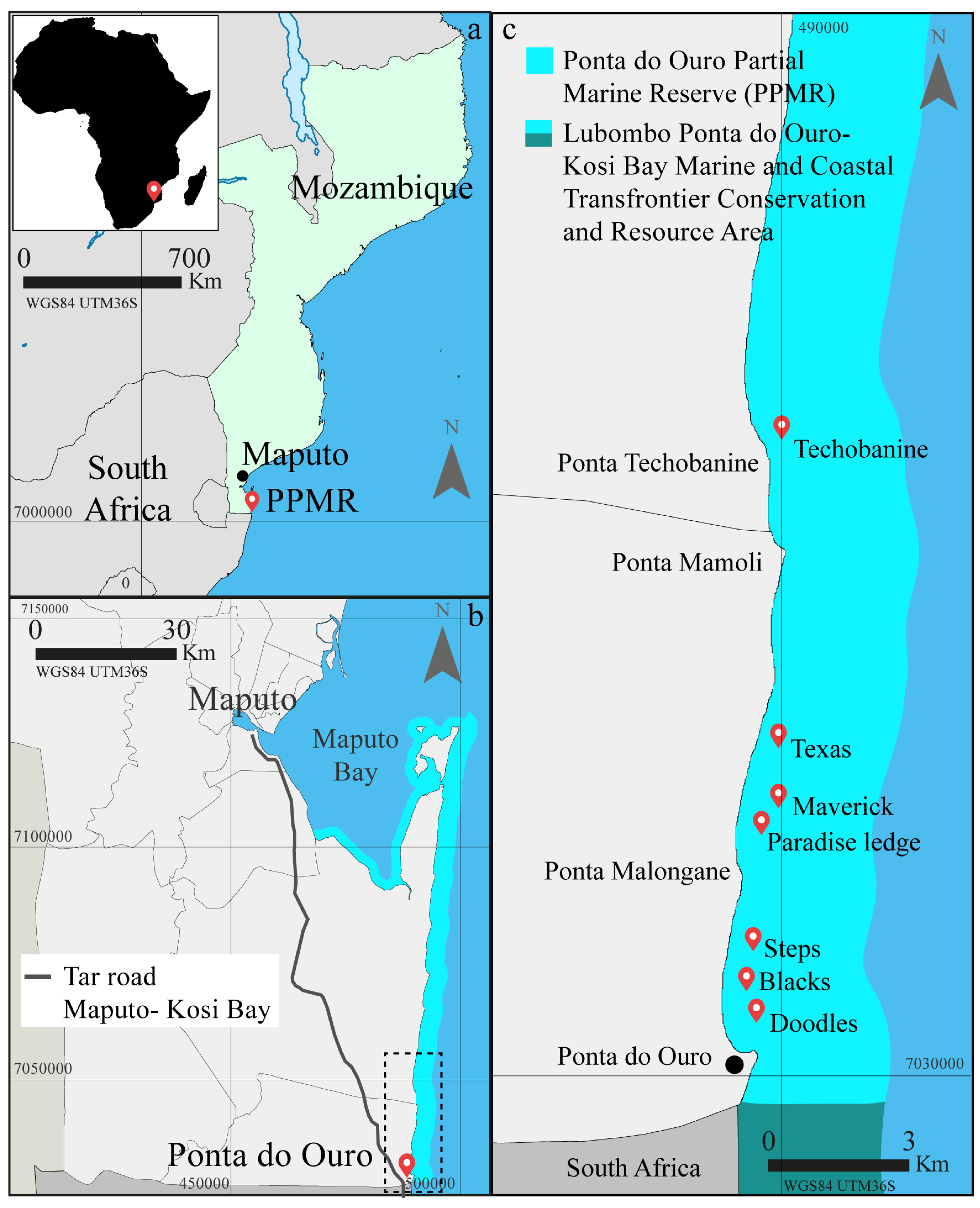
2.1. Study Area and Experimental Design

The study was conducted in the Ponta do Ouro Partial Marine Reserve (PPMR) (Mozambique). The protected area includes some of the southernmost coral reefs of the African continent (Figure 1), and is characterized by low profile outcrops originating from the fossilization of sand dunes that runs parallel to the coastline, and are covered by a non-accretive “coral carpet” and high numbers of endemic species [35,36,37,38,39]. High energy hydrodynamic conditions, characterizing the North-South coastline between Ilha da Inhaca and Ponta do Ouro, shape local topography and sediment transport [37,39,40]. As a result, studies have reported negligible impacts of climate change on Maputaland reefs compared to other reefs across the tropics, because of local hydrodynamic conditions (i.e., Agulhas current, local upwellings, and a swell-generated inshore counterflow) preventing extreme water heating [41,42,43]. Communities are often dominated by soft corals that are tolerant to strong wave energy and sediment re-suspension [19]. The PPMR is an international destination for scuba divers and nature tourism since the end of the civil war in the 1990s when 30k to 40k dives year −1 were recorded the 1995 [40], 80k–90k dives year −1 were recorded in 1998 [44] with 42.5k–62k dives year −1 were counted in 2001–2002 [45]. More recently, an average of 26k (± 3k) dives year −1 were reported by the PPMR (Table 2). In this study, seven dive sites were selected within a range of average depths comprised between −12 m to −25 m below mean sea level (BMSL), and areas between 425 m2 and 3500 m2. The number of divers year −1 ranged from none to >11k reported in the literature for 2001–2002 and 2011–2016 (Figure 1, Table 3).
High-resolution data were collected at each site in one single dive between April and June 2015 covering the entire coral reef area or surveying those areas commonly visited by divers at the larger study sites. Dive sites were mapped as in [23] using a modified Diver Propulsion Vehicle (DPV) equipped with action cameras (GoPro Hero3 Silver–Woodman Labs, Inc., San Mateo, CA, USA), a tablet (Asus Google Nexus 7 tablet—Google Inc., Mountain View, CA, USA), an illumination system and one GPS buoy (Garmin Ltd., Lenexa, KS, USA) (Figure 2). A detailed description of the vehicle in Palma et al. [23]. The camera was set to time-lapse mode, recording nadir images at 1 Hz frequency with a focal length equivalent to 21 mm. The position of each recorded image was estimated by coupling the camera recording time and the GPS clock [46]. The pitch, yaw and roll data of the sampling device were recorded logging the inertial navigation data obtained from the gyroscope and the accelerometer of the tablet and by using the UBICA Underwater Position System (UUPS) [47]. The geographic position of the sampling was recorded via a towed buoy with an integrated Etrex10 GPS (Garmin Ltd., Lenexa, KS, USA). PixGPS (BR Software, Asker, Norway) was used to tag the recorded images with the GPS positioning and the rotation data. The coordinates for each of the frames were used to georeference (scale, translate and rotate) the imagery into the coordinate system defined by the World Geodetic System (WGS84) and to minimize geometric distortions [48]. The Wide Area Augmentation System (WS) mode at 1 Hz frequency was used to record the position of the buoy. The diver maintained an average swimming speed of 0.75 m s −1 and an average distance to the sea bottom of 2.7 m, with the range being between 1.5 m and 3 m and with each frame covering 3 m2 (Figure 2a). The sampling path was adapted to the seascape characteristics to maximize overlapping images, by carrying out both parallel and perpendicular transects.

2.2. Data Processing

2.2.1. Photogrammetric Processing and Seascape Composition Analysis

For each site, high-resolution orthomosaics (pixel size < 0.01 m) were obtained by processing the geo-tagged images of the underwater surveys as in [23]. The Images were aligned to generate spare point cloud setting Photoscan version 1.4.1 (Agisoft LLC., St. Petersburg, Russia) [23] to high accuracy, generic pair selection, limiting the key points identification to 50,000 common features and unlimiting the number of the outcoming tie points cloud. Meshes were calculated setting the software surface type generation to height field, high face count and enabling interpolations. Adaptive orthomosaics texturing was used to export tiled (4096 pixels × 4096 pixels) georeferenced orthomosaics using the projected reference system Universal Transverse Mercator (UTM) fuse 36 Southern Hemisphere, defined by the World Geodetic System (WGS84).
First, the reef area belonging to solid substrate was digitalized using ArcGIS 10.1 software (Redlands, CA, USA). Then, to study the composition of the coral reefs at seascape scale, virtual random quadrats of 5 m × 5 m were randomly positioned three times over each ortho-mosaic (Figure 2b). The quadrat size 5 m × 5 m has proved to be representative of the coral reefs at the PPMR [23], and allowed to sample a minimum of 80% of hard substrates in all quadrat replicates and reef sites. The centroids of the virtual quadrats were distributed random in the reef sites using the ArcGIS tool “Create Random Points” (Redlands, CA, USA). We discarded the quadrats with more than 20% of their area outside the digitalized reef area [23]. Within each quadrat, the benthic organisms were identified in taxonomic and morphological classes, digitalized using ArcGIS 10.1 software (Redlands, CA, USA), and finally rasterized to obtain categorical maps (Table 4, Figure 2c1) [23].
The classes were summarized in functional groups (FGs, [19,50]) and for each class, abundance and the summary statistics of surface and perimeter were calculated and used for multivariate analysis (Figure 2c2,c3) (Section 2.2.2). FGs classes are based on a series of taxonomic, morphological, physiological, and behavioral characteristics reflecting adaptations to physical disturbance. “Resistant” to physical impacts organisms included sponges (SP), algal patches (TA) and “other invertebrates” (OI) (e.g., gastropods, tunicates, echinoderms, hexacorals Stichodactyla spp., Atriolum sp.). These taxa show high regenerative physiological resistance to physical damages because of their skeletal structure and have been often reported in relation to ecological shifts in coral reefs communities [2,51,52,53]. The “moderately resistant” organisms to physical impacts included soft corals (SCD, SCP, SCC, SCR, SCF) (e.g., Sarcophyton sp., Sinularia sp., Lobophyton spp.), massive corals (CM) (e.g., Platygyra spp., Montastrea spp., Galaxea spp., Favites spp., Favia spp. and Turbinaria sp.), folios corals (CF) (e.g., Montipora spp., Echinopora spp.), and encrusting corals (CE) (e.g., Porites spp.). Soft corals are often described as sensitive organisms to sediment burying and wave actions [54] but their flexibility of the colonies, their low profile suggest they are resistant animals to hydrodynamic condition [19]. Massive, encrusting and folios corals show resistance to physical impacts due to a stout or flat morphological growth. However, they can be dislodged or more commonly scratched by accidental impact with divers equipment [2,13,55]. Finally, the “fragile” “group included Acropora spp. (AC), branched corals (CB) (e.g., Pocillopora spp.), and tabular corals (CTA) (i.e., Turbinaria sp.). Acropora spp. and branched-coral taxa have tree-shaped carbonate skeletons that increase the structural complexity of reefs but, as erected forms, they are also the most exposed to breaks and fragmentation [2,11,12,55,56,57]. Among the fragile group, tabular corals and free-living fungiid colonies are the most subject to breaks, for example during severe weather conditions entire colonies might be tipped over [58].

2.2.2. Multivariate and Clustering Analysis

Data on FGs (i.e., diversity, surfaces and perimeter, average, maximal, minimal, standard deviation, count), and reef sites (i.e., depth, extension) were analyzed using a principal component analysis (PCA—[59]) and the distance-based clustering X-Means [60] to look for similarities in community composition between diving sites and possible diving impacts (Figure 2d,e). Data of number of dives per reef site were not included in the analysis. The approach, which involves a series of steps performed sequentially to the harmonized data was applied at seascape scale and carried out using the DataMiner system of the D4Science e-Infrastructure (Italy) [61,62].
First, a PCA was performed to reduce the dimensionality of the dataset and to explore the patterns in data variability among diving sites [59,63]. Secondly, X-Means was applied to the PCA-transformed vectors associated with the largest variance, to identify the variables indicating similarities of benthic composition between sites [63]. In this study, we searched for several clusters between 1 and 10, and applied a tolerance threshold of 25% over the centroids of the clusters that represent a summary of the characteristics of the cluster [63]. The clusters were evaluated with respect to expert opinion. Two independent experts evaluated the clusters by assigning the clusters’ results for each diving site. A confusion matrix was used to assess the agreement between the experts’ assessments and the X-Means clusters as the percentage of matching assignments (absolute percentage of agreement). The Cohen’s Kappa [64] was calculated to estimate the agreement between the experts and the model compared to purely random assignments [65]. To look at patterns of taxonomic and functional benthic composition over the clusters we used the categories in Table 4.

2.2.3. Estimation of Seascape Metrics

The composition of the reefs was investigated by calculating key seascape metrics such as diversity, aggregation and shape on the categorical maps using the FRAGSTATS v4 software (Amherst, MA, USA) [34]. The set of metrics was selected based on their relevance to seascape ecology composition. FRAGSTATS v4 computes a variety of metrics for categorical maps and has been used in a wide range of disciplines including seascape ecology [23,66,67,68,69]. In this study, the categorical maps were processed at patch (the single individual digitized in a polygon), class (taxonomical and morphological FGs, Table 4), and seascape level (denotes all the patches of different classes within the quadrats) by considering the disposition, the size and the shape of the patches within the quadrats. Patch density, Simpson Diversity Index, Patch Richness, Shannon’s diversity Index, Perimeter-Area Fractal Dimension, and Mean patch fractal dimension at seascape level, were compared between reef sites by applying a One-Way ANOVA test using the aov function in the R “stats” v3.5.1 package [70].
To address the ANOVA assumptions, particularly the assumption of heterogeneity in the residuals, Patch Density, Patch Richness, Simpson Diversity Index, Perimeter-Area Fractal Dimension were log-transformed, but this was not necessary for the rest of seascape metrics (Table 1). Validation of underlying assumptions of normality and homoscedasticity of tests residuals was applied following Zuur et al. [71] (shapiro.test function from the R “stats” v3.5.1 package [72] and leveneTest in R “car” v3.0-2 package [73]) and subsequently, post-hoc Tukey tests were applied to compare which specific treatments differ significantly using the TukeyHSD function from the R (New Zealand) “stats” v3.5.1 package [72].

3. Results

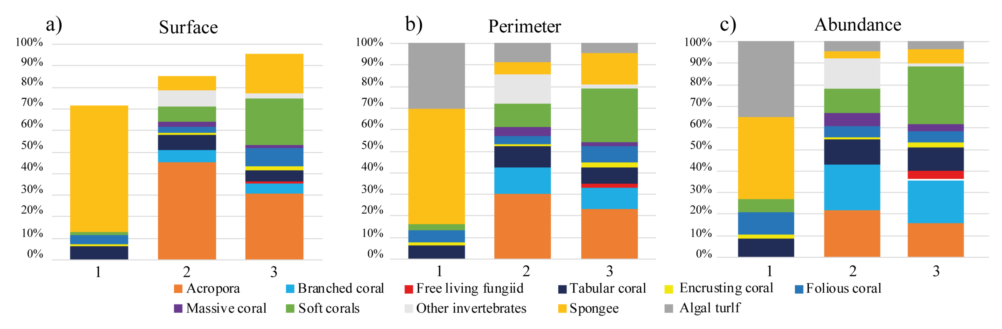
3.1. Seascape Composition of Diving Sites

Thousands of images were processed to generate the orthomosaics at each diving sites. 2102 images were aligned over 2186 for Doodle, 1165 images were aligned over 1190 for Blacks, 2108 images were aligned over 2165 for Steps, 1758 images were aligned over 1780 for Maverick, 2444 images were aligned over 2475 for Paradise Ledge, 1490 images were aligned over 1651 for Texas, and 3662 images were aligned over 3394 for Techobanine. From the analysis and digitalization of the orthomosaics, 11 functional groups were identified (Table 4). Doodles and Blacks showed the higher frequencies of sponges and algal patches among sites and lower abundances of organisms with <0.5 individual m−2 (Table 5). Steps presented an average density of 2.37 individual m−2 and was characterized by soft digitate and crested corals (SCD, SCC) and several classes of invertebrates (OI) including acidians and anemons. Branched coral (i.e., Pocillopora sp.) and Acropora were also present at site (Table 5). At Maverick and Paradise Ledge, organism densities averaged between 4.4 individual m−2 and 4.85 individual m−2 and soft corals (SCD, SCC, SCF, SCR) dominate the seascape. Acropora (ACS, ACD) and non-Acropora branched corals with folios and massive hard corals were also present (Table 5). Texas has the highest average density with 6.47 individual m−2 mainly represented by branched corals (CB), soft corals (SCD, SCC, SCR, SCF) and encrusting sponges (SPE). Tabular corals (CTU), Acroporas (ACS) and alges (TA) were also present (Table 5). Finally, Techobanine recorded 3.56 individual m−2 mainly represented by branched corals (ACC, CB, ACS), massive and tabular corals (CM, CTU) and soft corals (SCD, SCC, SCF) (Table 5).

3.2. Evaluation of Clusters and Agreement with the Experts

From the analysis, the reef was classified in three clusters, labelled, semantically described (Table 6), and evaluated with respect to expert opinion (Table 7). Clusters evaluation showed moderate to a substantial agreement with expert opinion, indicating reliable semantic interpretations of the vectors identified in the clusters variations (Table 7). The marginal agreement is recorded between the two experts due to Expert 2 who classified most of the sites as moderately impacted.
Cluster number 1 groups very impacted sites (Doodles and Blacks) and contains 23 vectors. It indicates the whole set of benthic taxa that are very resistant and resilient to physical pressures (i.e., algae, sponges), with low density and diversity, and generally more complex morphological shapes per organism.
Moderately impacted cluster (Cluster 2) contains 33 vectors and three sites (Steps, Techobanine and Texas). It represents the set of taxa that are low resistant but highly resilient to pressures, i.e., branched hard coral. They are sensitive to breaks but they have high growth rates [74] and show higher density and diversity, lower morphological complexity per organism and higher fractal complexity at seascape scale than cluster 1 (Figure 3 and Figure 4).
Finally, the low impacted cluster (cluster 3) describes 32 vectors and two sites (Paradise ledge and Maverick). It refers to taxa that are moderately resistant and low resilient to physical pressures (i.e., soft corals that have low growth rate and low recruitment rate but highly resistant to high energy hydrodynamic conditions [19]), show the highest level of taxa diversity and density, and a high level of fractal complexity at seascape scale.
Very impacted sites (cluster 1) showed the greatest patch surfaces, and similar distribution to moderately impacted sites (cluster 2, Figure 3a and Figure 4). Doodles and Blacks (cluster 1) were also characterized by patches with larger perimeters and higher variability in the first and third quartile than Steps, Techobanine, Texas (cluster 2), Paradise ledge and Maverick (cluster 3) (Figure 3b and Figure 4). In fact, sites in clusters 2 and 3 were characterized by patches with smaller perimeters and lower variabilities (Figure 3b and Figure 4). The low impacted sites (cluster 3) showed the highest abundance of benthic organisms and high variability among the two sites (Figure 3c and Figure 4). Conversely, in very and moderately impacted sites, organism abundances have overall similar distributions among sites (cluster 1 and 2, Figure 3a,c and Figure 4).
Across sites, the resistant group accounted for >85% of the patches surface, the 80% of their perimeter and more than >60% in abundances in the very impacted cluster (Figure 5a,b). Moderately resistant organisms constituted only the 10% of the patches surface at very impacted cluster, while contributed >30% in the moderately and more than 60% in the low impacted clusters (Figure 5a). The moderately resistant group had a similar pattern also for patches perimeter and abundances (Figure 5b,c).
Among sites, the resistant group had the highest contribution in percentage to mean patch areas and abundances to Blacks (95%), Doodle (>75%), and Steps (>50%) (Figure 6 and Figure 7). The moderately fragile group mostly accounted in percentage to mean patch areas and abundances to Paradise Ledge (50%), Maverick (70%), and Texas (60%) (Figure 7 and Figure 8). Finally, Paradise Ledge and Techobanine showed the highest contribution in percentage to mean patch areas (45% in Paradise Ledge, 70% in Techobanine) of the fragile organisms group (Figure 7 and Figure 8).

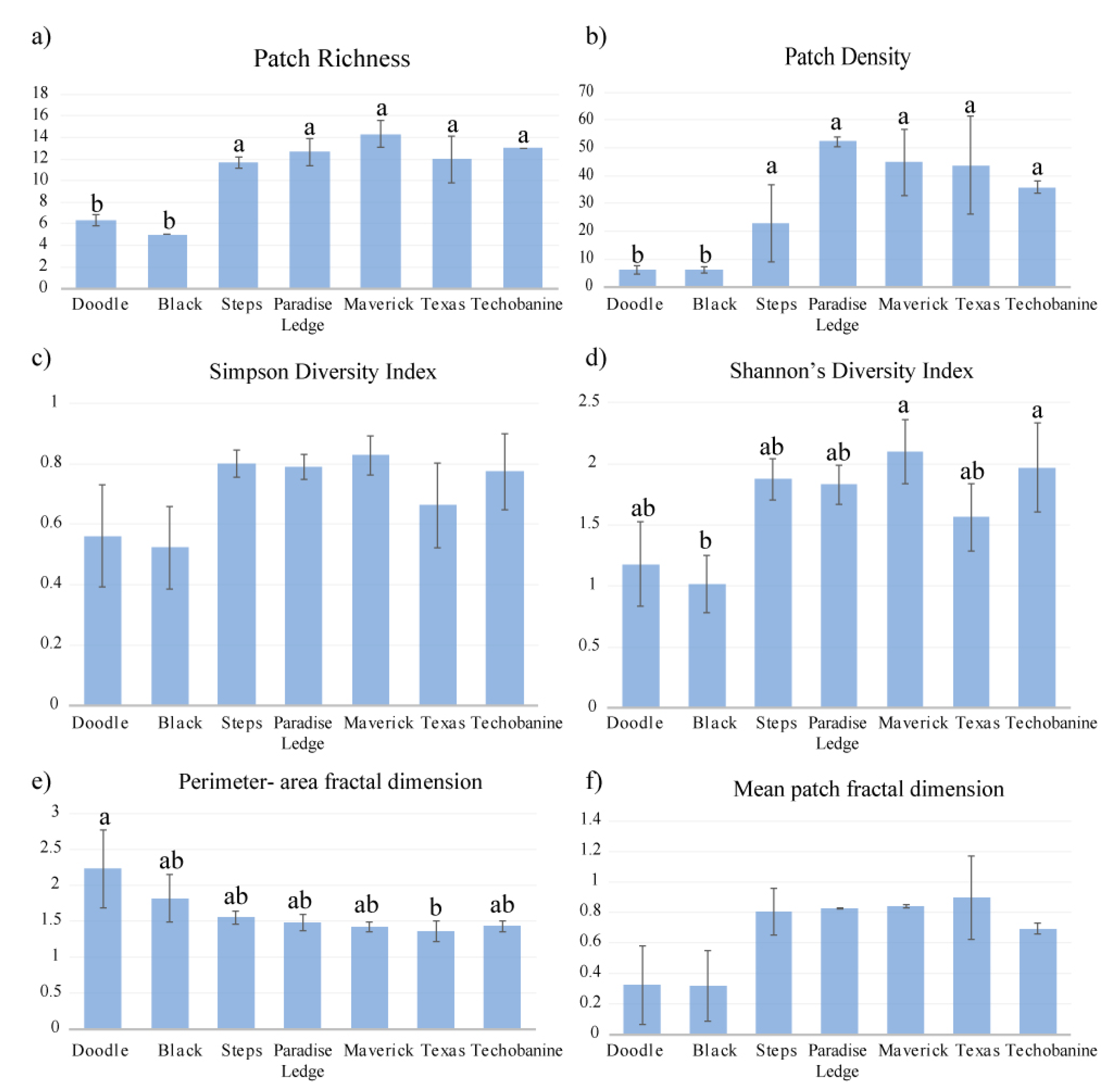
3.3. Seascape Metrics

Most of the seascape metrics were significantly different across reefs (i.e., patch richness, patch density, Shannon’s diversity index and perimeter-area fractal dimension), except for the Simpson Diversity Index and the mean patch fractal dimension index. These indices indicated a similar average complexity of organisms across the seascapes. (Figure 9). Patch density, patch richness and Shannon’s Diversity Index lowered at very impacted sites (cluster 1, Blacks and Doodle) (Figure 9). Patch density showed significant differences (F(6,14) = 23.04, p < 0.01) between sites with larger seascape complexity at Paradise Ledge (52 ± 1.8 organisms) and lower at Black (6 ± 1.0 patches) and Doodles (6 ± 1.5 patches) (Figure 9). Patch richness exhibited significant differences in the number of classes of organisms between sites (F(6,14) = 37.40, p < 0.01), with five classes at Black 5 (±0.4) and Doodle 6 (±0.4) and over 10 in the other diving sites (Figure 9). SDHI index indicates that Maverick and Techobanine have higher number of classes of organisms, equally distributed within the sites, than the other sites (Figure 9). Finally, Doodle has the highest morphological complexity of the patches (2.23 ± 0.54) associated (perimeter-area fractal dimension index F(6,14) = 3.54, p = 0.02) (Figure 9).

4. Discussion

This research assessed the spatial composition of benthic reef communities at seascape scale and within recreational diving sites using SfM orthomosaics. Coral reefs exhibited different spatial compositions of benthic communities, with patterns emerging between diving sites. In this section, we discuss the variation of taxonomic and functional descriptors across diving sites (Section 4.1), and the potential applications of the proposed approach (Section 4.2).

4.1. Linking Spatial Benthic Composition to Recreational Diving Sites

Differences between sites were recorded by FGs and their metrics (i.e., surface, perimeter, abundance) in the clusters, indicating that scuba diving and local environmental conditions could influence the resultant spatial community structures and that specific taxonomic and functional descriptors provide further insight into the factors affecting coral reefs. The seascape indices did not show significant variability within sites suggesting that the selected sampling units and the number of replicates were suitable for describing the communities of the selected coral reefs. The resistant-to-physical-impact categories provided further insights into seascape composition, and partially support our second hypothesis that the contribution of resistant organism tend to occur in small, shallow and highly dived coral reef sites (Figure 9).
Dimensional factors, such as patch surface and perimeter are indicators of benthic assemblage composition and spatial complexity. The larger the organism, the higher is its planar complexity as a result of intra- and inter-species competition within the seascape [75]. The seascape composition factors (i.e., functional groups and abundance), are indicators of benthic taxa diversity and organisms density. Lower values in taxa diversity are related to more homogeneous seascapes, whereas higher values of organism densities suggested lower human impacts (i.e., low number of dives per year) and environmental pressures (i.e., deeper and larger coral reefs).
Low densities of organisms with large and complex shapes were recorded in Doodle and Blacks which were grouped in the very impacted cluster (cluster 1). These sites are characterized by lower taxa diversity and by the highest number of dives per year and are the closest sites to the launching point on Ponta do Ouro beach. Doodle has been highly frequented since 1995 while Blacks has been dived since 2011 with moderately intensities (Table 3). Both sites are subjected to strong environmental pressures due the number of dives per year in relation to small surface areas (450 m2 to 850 m2) at moderately shallow average depth (−17 m to −19 m). The waves and the abrasive action of re-suspended sediment limit the settlement and growth of resistant-to-physical-impact organisms such as sponges and algae. Previous studies have demonstrated that the high-amplitude swells originating in the Southern Ocean [35,55,76] promote suspension and deposition of sediment, mechanisms of abrasions that limit at the reef–sediments interface the recruitments of benthic larvae, also for resistant-to-physical pressure taxa [19]. Doodles and Blacks also presented the highest frequencies of organisms resistant to physical impacts (i.e., sponges, algal patches). The few fragile organisms identified in cluster 1 sites are tabular corals which have a limited three-dimensional complexity shape and are potentially more resistant to the physical impacts of scuba diving than Acroporas and similar branched corals.
Higher FGs diversity and a high presence of Acropora colonies were recorded for the moderately impacted cluster (cluster 2). This cluster included three sites very distant from each other (Figure 1): Techobanine is at 19.6 km, Steps at 3.6 km and Texas at 9.6 km from the Ponta do Ouro launching point. Steps is characterized by the lowest organisms’ density while Texas has the highest. Both sites present high variability which suggests that there are spatial differences in the benthic community composition (patch richness and patch density) over the sampled seascapes (Figure 9). Texas also showed smaller average organism surface and higher fractal dimensions than the other two sites, suggesting greater variability in the shapes and dimensions of organisms that could be related to the habitat recovering from extreme environmental events (i.e., cyclones and storms) or to intense scuba diving of the particular site in the past (Table 2). Techobanine showed the highest frequency of hard branched corals and colonies of Acroporas, probably favored by the lower average depth of the site (−12 m) and by the very low number of dives per years recorded in the last decade. The low density and large dimensions of the organisms is explained by the higher growth rate of these hard corals [77] which mitigates the impacts caused by the high energy hydrodynamic conditions of the area.
Among cluster 2, Steps is the only site with high number of scuba dives since 1995 (>3000 dives year−1), while Texas has less than 300 dives year−1 in the last decade and Techobanine is annually rarely visited (Table 2 and Table 3). Steps is smaller than Techobanine and Texas, but it develops along a rocky edge. There are small canyons and cracks in the rocky substrate which provide sheltered areas against waves action and scuba diving direct impacts, resulting in a more heterogeneous community with moderately fragile and resistant organisms [78]. Cluster 3 showed higher level of taxa diversity and organism density probably as a result of the low scuba-diving pressure and the more benign environmental conditions. The reefs are characterized by several sizes of corals, small perimeter variability and low fractality within the landscape. Paradise ledge and Maverick are the deepest (−18 m to −20 m) and largest sites, with an average of 365 dive year−1 at Paradise Ledge in the last 12 years. Maverick is a rarely dived site close to Paradise Ledge.

4.2. Implications for Reef Management

This study proposes a new transferable approach based on SfM to study the spatial composition of coral communities and contributes towards the identification of reefs where diving activities are impacting on the community structure.
Those responsible for managing reefs are increasingly considering both the revenue derived from scuba diving as well as the impacts on the habitats in their management plans as it is one of the most profitable activities in marine parks [79]. Global policies are needed to face the challenges of global warming and consequently massive bleaching events on reefs [80]. However, more local actions are needed to preserve and manage the reefs in terms of the impacts caused by human activities. There is therefore a clear need to provide marine managers with cost effective and easily deployable approaches that can be applied to coral reefs.
Our method is the first to provide relevant, cost effective information to marine managers that will enable them to study the changes in composition and functionality across reefs at PPMR. It will provide an objective basis for conservation actions and long-term data collection programs.
Recently, the village of Ponta do Ouro has been connected via a new road to Maputo. The new road has reduced the travel time to less than two hours by car or buses while previously it was a 7 h journey in an all-terrain vehicle. Managers of the PPMR are expecting greater numbers of visitors with consequent negative impacts on the local natural habitats including the coral reefs (personal communication from the Director of the Ponta do Ouro Partial Marine Reserve). It will be important for the PPMR managers to establish and document a baseline condition survey of all the potentially affected reefs. This can be carried out quickly and cost effectively with the method we have developed. The seascape approach will also facilitate the development of a prioritized action plan. It will require the collection of quantitative, georeferenced, and representative samples, including compositional data to provide a functional perspective. The SfM-based approach applied in this way will leads to a better understanding of the short, medium and long-term implications of benthic changes to management actions.
Managers of the PPMR can benefit from the combined SfM-approach and statistical classification at any stage of the analysis. First looking at the clusters that describe: (i) taxonomic and morphologic composition of the benthic communities, (ii) seascape spatial composition and organism shape complexity, (iii) classes of fragility to physical impacts. Second by looking at the final matrices which embed the summary of the related ecological data and provide insights into the spatial variability of the coral reef benthic communities in the protected area. From the above information, managers of the PPMR can prioritize conservation measures at each site.
The information collected in this study has indicated the need for further data collection and analysis if the overall management of the reefs is to be effective and to ensure that the methodology developed is able to inform the most appropriate management approaches for the reefs. This includes: establishing a baseline before there is an increase in people visiting the area; identifying the magnitude of the various risks to the extent and condition of the reefs; distinguishing between the impacts caused by the various factors for example natural variability by season and by year, human impacts from diving, environmental pressures from natural events such as storms, climate change; determining the relative impact of the different factors for each location. This information would then enable appropriate risk management approaches to be developed. These could include: restricting the numbers of dives allowed at certain locations and during particular environmental conditions; allowing recovery periods for areas where no diving is allowed; access for beginners being restricted to particular areas; clear instructions and educational programs for divers and those running diving schools so that they are aware of and avoid certain activities known to cause damage [81]. To this end, information collected from scuba diving can support marine conservation in the context of marine citizen science [82]. Trained divers involved in monitoring programs (i.e., Reef Check) have reduced cost, time, equipment and simplified logistics [83,84]. In this direction, recreational diving represents a potential to continue monitoring and surveillance programs [82], and could be an opportunity to promote photogrammetry at seascape scale to ensure that the risk mitigation approaches are effective. The monitoring approach we have developed can play an essential role within the overall reef management approach. The monitoring approach needs to include: determining the baseline conditions; identifying and distinguishing between the risks to the condition of the reefs from all sources; introducing appropriate reef management actions; periodic monitoring to ensure that the management measures are being effective and modifying them as required; long-term monitoring to assess natural variability and the impact of underlying long-term environmental changes and pressures.

5. Conclusions

This study has reported the application of SfM-based approach to marine habitats and its advantages. SfM demonstrated to be a flexible, affordable and reliable technology for rapid surveys, providing informative data to support spatial analysis of ecological communities and to investigate the effects of human stressors. Our results showed:
  • substantial agreement with expert opinions;
  • differences in the benthic composition between diving sites in terms of: (i) organism diversity, surface, perimeter, abundance, (ii) functional groups categories (e.g., resistant, moderately resistant, fragile);
  • Resistant-to-physical-impact categories (i.e., sponges and algae) were most abundant at small diving sites and highly visited by divers. These sites were characterized by big organisms and with complex shapes, low taxa diversity and density.
  • Fragile-to-physical-impact categories (i.e., Acropora spp.) were most abundant at diving sites low or moderately visited by divers. These sites are characterized by complex geomorphology and moderate hydrodynamic conditions.
  • The highest taxa diversity and density, and the lowest abundance of resistant-to-physical-impact FGs were recorded at large and rarely dived sites. The sites exhibited different seascape metrics (i.e., patch density, patch richness, Shannon Diversity Index, Perimeter-Area Fractal Index), with general patterns emerging in terms of responses to diving pressure and environmental conditions.
To conclude, this study suggests that having effective coral ecosystem management systems in place at PPMR will be essential if these important marine habitats are to survive and flourish. This is especially the case with the potential significant increase in human impacts arising from the increasing accessibility of the area to visitors. By focusing on strengthening the resilience of marine ecosystems at a seascape scale, marine management can optimize goods and services as new environmental challenges arise [85,86].

Author Contributions

M.P. conceived, designed and analyzed the datasets. C.M. contributed to the data analysis and writing of the manuscript. M.R.C. and P.L. contributed to editing and revising the manuscript. U.P. and J.F. assessed the clusters. G.C. and C.C. provided their statistical and ecological perspectives and revised the manuscript. All authors read and approved the manuscript.

Funding

This work was supported by the PhD scholarship EUREKA, the European Social Funds (FSE), Programma Operativo Regionale (POR) 2014/2020 Regione Marche (Italy), the Marie Sklodowska-Curie Action, Horizon2020 within the project GreenBubbles (G.A.643712), and UBICA s.r.l.

Conflicts of Interest

The authors declare no conflict of interest.

References

  1. Luna, B.; Pérez, C.V.; Sánchez-Lizaso, J.L. Benthic impacts of recreational divers in a Mediterranean Marine Protected Area. ICES J. Mar. Sci. 2009, 66, 517–523. [Google Scholar] [CrossRef]
  2. Lyons, P.J.; Arboleda, E.; Benkwitt, C.E.; Davis, B.; Gleason, M.; Howe, C.; Mathe, J.; Middleton, J.; Sikowitz, N.; Untersteggaber, L.; et al. The effect of recreational SCUBA divers on the structural complexity and benthic assemblage of a Caribbean coral reef. Biodivers. Conserv. 2015, 24, 3491–3504. [Google Scholar] [CrossRef]
  3. Bravo, G.; Márquez, F.; Marzinelli, E.M.; Mendez, M.M.; Bigatti, G. Effect of recreational diving on Patagonian rocky reefs. Mar. Environ. Res. 2015, 104, 31–36. [Google Scholar] [CrossRef] [PubMed]
  4. Richardson, D. A brief history of recreational diving in the United States. South Pacific Underw. Med. Soc. 1999, 29. [Google Scholar]
  5. Buckley, R. Sustainable tourism: Research and reality. Ann. Tour. Res. 2012, 39, 528–546. [Google Scholar] [CrossRef] [Green Version]
  6. Dimmock, K.; Musa, G. Scuba diving tourism system: A framework for collaborative management and sustainability. Mar. Policy 2015, 54, 52–58. [Google Scholar] [CrossRef] [Green Version]
  7. Roche, R.C.; Harvey, C.V.; Harvey, J.J.; Kavanagh, A.P.; McDonald, M.; Stein-Rostaing, V.R.; Turner, J.R. Recreational diving impacts on coral reefs and the adoption of environmentally responsible practices within the SCUBA diving industry. Environ. Manag. 2016, 58, 107–116. [Google Scholar] [CrossRef] [Green Version]
  8. Lucrezi, S.; Saayman, M. Sustainable scuba diving tourism and resource use: Perspectives and experiences of operators in Mozambique and Italy. J. Clean. Prod. 2017, 168, 632–644. [Google Scholar] [CrossRef]
  9. Rogers, C.S. Responses of coral reefs and reef organisms to sedimentation. Mar. Ecol. Progress Ser. Oldendorf 1990, 62, 185–202. [Google Scholar] [CrossRef]
  10. Dikou, A.; Van Woesik, R. Survival under chronic stress from sediment load: Spatial patterns of hard coral communities in the southern islands of Singapore. Mar. Pollut. Bull. 2006, 52, 1340–1354. [Google Scholar] [CrossRef]
  11. Hawkins, J.P.; Roberts, C.M. Effects of recreational SCUBA diving on fore-reef slope communities of coral reefs. Biol. Conserv. 1992, 62, 171–178. [Google Scholar] [CrossRef]
  12. Chadwick-Furman, N. Effects of SCUBA diving on coral reef invertebrates in the US Virgin Islands: Implications for the management of diving. In Proceedings of the 6th International Conference on Coelenterate Biology, Noordwijkerhout, The Netherlands, 16–21 July 1995; Volume 91, pp. 1–5. [Google Scholar]
  13. Zakai, D.; Chadwick-Furman, N.E. Impacts of intensive recreational diving on reef corals at Eilat, northern Red Sea. Biol. Conserv. 2002, 105, 179–187. [Google Scholar] [CrossRef]
  14. Erftemeijer, P.L.; Riegl, B.; Hoeksema, B.W.; Todd, P.A. Environmental impacts of dredging and other sediment disturbances on corals: A review. Mar. Poll. Bull. 2012, 64, 1737–1765. [Google Scholar] [CrossRef] [PubMed]
  15. Lamb, J.B.; True, J.D.; Piromvaragorn, S.; Willis, B.L. Scuba diving damage and intensity of tourist activities increases coral disease prevalence. Biol. Conserv. 2014, 178, 88–96. [Google Scholar] [CrossRef]
  16. Wilkinson, C.R.; Green, A.; Almany, J.; Dionne, S. Monitoring Coral Reef Marine Protected Areas: A Practical Guide On How Monitoring Can Support Effective Management of MPAs; Australian Institute of Marine Science and the IUCN Marine Program: Townsville, Australia, 2003. [Google Scholar]
  17. Hill, J.; Wilkinson, C. Methods for ecological monitoring of coral reefs. Aust. Inst. Mar. Sci. Townsville 2004, 117, 1–116. [Google Scholar]
  18. Salm, R.V. Coral reefs and tourist carrying capacity; the Indian Ocean experience. Ind. Environ. 1986, 9, 11–14. [Google Scholar]
  19. Schleyer, M.; Celliers, L. Coral dominance at the reef–sediment interface in marginal coral communities at Sodwana Bay, South Africa. Mar. Freshw. Res. 2003, 54, 967–972. [Google Scholar] [CrossRef]
  20. Meesters, E.; Bos, A.; Gast, G. Effects of sedimentation and lesion position on coral tissue regeneration. In Proceedings of the Seventh International Coral Reef Symposium, Guam, Micronesia, 22–27 June 1992; Volume 2, pp. 681–688. [Google Scholar]
  21. Boström, C.; Pittman, S.J.; Simenstad, C.; Kneib, R.T. Seascape ecology of coastal biogenic habitats: Advances, gaps, and challenges. Mar. Ecol. Progress Ser. 2011, 427, 191–217. [Google Scholar] [CrossRef] [Green Version]
  22. Cruz-Vázquez, C.; Rioja-Nieto, R.; Enriquez, C. Spatial and temporal effects of management on the reef seascape of a marine protected area in the Mexican Caribbean. Ocean Coast. Manag. 2019, 169, 50–57. [Google Scholar] [CrossRef]
  23. Palma, M.; Rivas Casado, M.; Pantaleo, U.; Cerrano, C. High resolution orthomosaics of African coral reefs: A tool for wide-scale benthic monitoring. Remote Sens. 2017, 9, 705. [Google Scholar] [CrossRef] [Green Version]
  24. Westoby, M.; Brasington, J.; Glasser, N.; Hambrey, M.; Reynolds, J. ‘Structure-from-Motion’ photogrammetry: A low-cost, effective tool for geoscience applications. Geomorphology 2012, 179, 300–314. [Google Scholar] [CrossRef] [Green Version]
  25. Ferrari, R.; Figueira, W.F.; Pratchett, M.S.; Boube, T.; Adam, A.; Kobelkowsky-Vidrio, T.; Doo, S.S.; Atwood, T.B.; Byrne, M. 3D photogrammetry quantifies growth and external erosion of individual coral colonies and skeletons. Sci. Rep. 2017, 7, 16737. [Google Scholar] [CrossRef] [PubMed]
  26. Figueira, W.; Ferrari, R.; Weatherby, E.; Porter, A.; Hawes, S.; Byrne, M. Accuracy and precision of habitat structural complexity metrics derived from underwater photogrammetry. Remote Sens. 2015, 7, 16883–16900. [Google Scholar] [CrossRef] [Green Version]
  27. Storlazzi, C.D.; Dartnell, P.; Hatcher, G.A.; Gibbs, A.E. End of the chain? Rugosity and fine-scale bathymetry from existing underwater digital imagery using Structure-from-Motion (SfM) technology. Coral Reefs 2016, 35, 889–894. [Google Scholar] [CrossRef]
  28. Ferrari, R.; Bryson, M.; Bridge, T.; Hustache, J.; Williams, S.B.; Byrne, M.; Figueira, W. Quantifying the response of structural complexity and community composition to environmental change in marine communities. Glob. Chang. Biol. 2016, 22, 1965–1975. [Google Scholar] [CrossRef]
  29. Coro, G.; Palma, M.; Ellenbroek, A.; Panichi, G.; Nair, T.; Pagano, P. Reconstructing 3D virtual environments within a collaborative e-infrastructure. Concurr. Comput. Pract. Exp. 2018, 31, e5028. [Google Scholar] [CrossRef]
  30. Burns, J.; Delparte, D.; Kapono, L.; Belt, M.; Gates, R.; Takabayashi, M. Assessing the impact of acute disturbances on the structure and composition of a coral community using innovative 3D reconstruction tech-niques. Methods Oceanogr. 2016, 15, 49–59. [Google Scholar] [CrossRef] [Green Version]
  31. Raoult, V.; David, P.A.; Dupont, S.F.; Mathewson, C.P.; O’Neill, S.J.; Powell, N.N.; Wil-liamson, J.E. GoPros™ as an underwater photogrammetry tool for citizen science. PeerJ 2016, 4, e1960. [Google Scholar] [CrossRef]
  32. Spellerberg, I.F.; Fedor, P.J. A tribute to Claude Shannon (1916–2001) and a plea for more rigorous use of species richness, species diversity and the ‘Shannon–Wiener’Index. Glob. Ecol. Biogeogr. 2003, 12, 177–179. [Google Scholar] [CrossRef] [Green Version]
  33. Somerfield, P.; Clarke, K.; Warwick, R. Simpson index. In Encyclopedia of Ecology; Elsevier: Oxford, UK, 2008. [Google Scholar]
  34. McGarigal, K. FRAGSTATS help. Doc. FRAGSTATS 2014, 4, 1–182. [Google Scholar]
  35. Ramsay, P. Marine geology of the Sodwana Bay shelf, southeast Africa. Mar. Geol. 1994, 120, 225–247. [Google Scholar] [CrossRef]
  36. Ramsay, P. Quaternary marine geology of the Sodwana Bay continental shelf, northern KwaZulu-Natal. Oceanogr. Lit. Rev. 1996, 11, 1103. [Google Scholar]
  37. Jordan, I.E.; Samways, M.J. Recent changes in coral assemblages of a South African coral reef, with recommendations for long-term monitoring. Biodivers. Conserv. 2001, 10, 1027–1037. [Google Scholar] [CrossRef]
  38. Riegl, B. Taxonomy and Ecology of South African Reef Corals. Ph.D. Thesis, University of Cape Town, Cape Town, South Africa, 1993. [Google Scholar]
  39. Celliers, L.; Schleyer, M.H. Coral community structure and risk assessment of high-latitude reefs at Sodwana Bay, South Africa. Biodivers. Conserv. 2008, 17, 3097–3117. [Google Scholar] [CrossRef]
  40. Robertson, W.; Schleyer, M.; Fielding, P.; Tomalin, B.; Beckley, L.; Fennessy, S.; Van der Elst, R.; Bandeira, S.; Macia, A.; Gove, D. Inshore Marine Resources and Associated Opportunities For Development of the Coast of Southern Mozambique: Ponta do Ouro to Cabo de Santa Maria; Oceanographic Research Institute: Durban, South Africa; Volume 130, pp. 1–51, Unpublished Report.
  41. Ramsay, P.; Cooper, J.; Wright, C.; Mason, T. The occurrence and formation of ladderback ripples in subtidal, shallow-marine sands, Zululand, South Africa. Mari. Geol. 1989, 86, 229–235. [Google Scholar] [CrossRef]
  42. Riegl, B. Climate change and coral reefs: Different effects in two high-latitude areas (Arabian Gulf, South Africa). Coral Reefs 2003, 22, 433–446. [Google Scholar] [CrossRef]
  43. Riegl, B.; Piller, W.E. Possible refugia for reefs in times of environmental stress. Int. J. Earth Sci. 2003, 92, 520–531. [Google Scholar] [CrossRef]
  44. Motta, H.; Rodrigues, M.; Schleyer, M. Coral reef monitoring and management in Mozambique. In Coral Reef Degradation in the Indian Ocean: Status Report; CORDIO, SAREC Marine Science Program Department of Zoology Stockholm University: Stockholm, Sweden, 2000; pp. 43–48. [Google Scholar]
  45. Costa, A.; Pereira, M.A.; Motta, H.; Schleyer, M. Status of coral reefs of Mozambique: 2004. In Coral Reef Degradation in the Indian Ocean: Status Report; CORDIO, SAREC Marine Science Program Department of Zoology Stockholm University: Stockholm, Sweden, 2005; pp. 54–60. [Google Scholar]
  46. Roelfsema, C.; Phinn, S.; Jupiter, S.; Comley, J.; Albert, S. Mapping coral reefs at reef to reef-system scales, 10s–1000s km2, using object-based image analysis. Int. J. Remote. Sens. 2013, 34, 6367–6388. [Google Scholar] [CrossRef]
  47. Ferraris, D.; Palma, M.; Pantaleo, U.; Cerrano, C.; Chiantore, M. Method and Device for Tracking the Path of an Object. WO Patent App. PCT/IB2016/053,924, 5 January 2017. [Google Scholar]
  48. Palma, M.; Rivas Casado, M.; Pantaleo, U.; Pavoni, G.; Pica, D.; Cerrano, C. SfM-Based Method to Assess Gorgonian Forests (Paramuricea clavata (Cnidaria, Octocorallia)). Remote Sens. 2018, 10, 1154. [Google Scholar] [CrossRef] [Green Version]
  49. Peraira, M.A.; Schleyer, M.H. A diver and diving survey in southern Mozambique. In Coral Reef Degrad. Indian Ocean: Status Report; CORDIO, SAREC Marine Science Program Department of Zoology Stockholm University: Stockholm, Sweden, 2005; pp. 184–192. [Google Scholar]
  50. Edinger, E.N.; Risk, M.J. Reef classification by coral morphology predicts coral reef conservation value. Biol. Conserv. 2000, 92, 1–13. [Google Scholar] [CrossRef]
  51. Hughes, T.P.; Baird, A.H.; Bellwood, D.R.; Card, M.; Connolly, S.R.; Folke, C.; Grosberg, R.; Hoegh-Guldberg, O.; Jackson, J.B.; Kleypas, J.; et al. Climate change, human impacts, and the resilience of coral reefs. Science 2003, 301, 929–933. [Google Scholar] [CrossRef] [PubMed] [Green Version]
  52. Wulff, J. Resistance vs recovery: Morphological strategies of coral reef sponges. Funct. Ecol. 2006, 20, 699–708. [Google Scholar] [CrossRef]
  53. Norström, A.V.; Nyström, M.; Lokrantz, J.; Folke, C. Alternative states on coral reefs: Beyond coral–macroalgal phase shifts. Mar. Ecol. Progress Ser. 2009, 376, 295–306. [Google Scholar] [CrossRef]
  54. Riegl, B.; Schleyer, M.H.; Cook, P.; Branch, G. Structure of Africa’s southernmost coral communities. Bull. Mar. Sci. 1995, 56, 676–691. [Google Scholar]
  55. Schleyer, M.H.; Tomalin, B.J. Damage on South African coral reefs and an assessment of their sustainable diving capacity using a fisheries approach. Bull. Mar. Sci. 2000, 67, 1025–1042. [Google Scholar]
  56. Rouphael, T.; Inglis, G. The effects of qualified recreational SCUBA divers on coral reefs. Tech. Rep. CRC Reef Res. Cent. 1995, 4, 39. [Google Scholar]
  57. Floros, C.; Schleyer, M. The functional importance of Acropora austera as nursery areas for juvenile reef fish on South African coral reefs. Coral Reefs 2017, 36, 139–149. [Google Scholar] [CrossRef]
  58. Hughes, T.; Connell, J. Multiple stressors on coral reefs: A long-term perspective. Limnol. Oceanogr. 1999, 44, 932–940. [Google Scholar] [CrossRef]
  59. Jolliffe, I. Available online: https://onlinelibrary.wiley.com/doi/abs/10.1002/0470013192.bsa501 (accessed on 16 October 2019).
  60. Pelleg, D.; Moore, A.W. X-means: Extending k-means with efficient estimation of the number of clusters. Icml 2000, 1, 727–734. [Google Scholar]
  61. Coro, G.; Candela, L.; Pagano, P.; Italiano, A.; Liccardo, L. Parallelizing the execution of native data mining algorithms for computational biology. Concurr. Comput. Pract. Exp. 2015, 27, 4630–4644. [Google Scholar] [CrossRef]
  62. Coro, G.; Panichi, G.; Scarponi, P.; Pagano, P. Cloud computing in a distributed e-infrastructure using the web processing service standard. Concurr. Comput. Pract. Exp. 2017, 29, e4219. [Google Scholar] [CrossRef]
  63. Magliozzi, C.; Coro, G.; Grabowski, R.; Packman, A.I.; Krause, S. A multiscale statistical method to identify potential areas of hyporheic exchange for river restoration planning. Environ. Modell. Softw. 2019, 111, 311–323. [Google Scholar] [CrossRef] [Green Version]
  64. Cohen, J. A coefficient of agreement for nominal scales. Educ. Psychol. Measur. 1960, 20, 37–46. [Google Scholar] [CrossRef]
  65. Coro, G.; Webb, T.J.; Appeltans, W.; Bailly, N.; Cattrijsse, A.; Pagano, P. Classifying degrees of species commonness: North Sea fish as a case study. Ecol. Modell. 2015, 312, 272–280. [Google Scholar] [CrossRef] [Green Version]
  66. Garrabou, J.; Riera, J.; Zabala, M. Landscape pattern indices applied to Mediterranean subtidal rocky benthic communities. Landsc. Ecol. 1998, 13, 225–247. [Google Scholar] [CrossRef]
  67. Teixido, N.; Garrabou, J.; Arntz, W. Spatial pattern quantification of Antarctic benthic communities using landscape indices. Mar. Ecol. Progress Ser. 2002, 242, 1–14. [Google Scholar] [CrossRef]
  68. Kendall, M.S.; Miller, T. The influence of thematic and spatial resolution on maps of a coral reef ecosystem. Mar. Geodesy 2008, 31, 75–102. [Google Scholar] [CrossRef]
  69. Wedding, L.M.; Lepczyk, C.A.; Pittman, S.J.; Friedlander, A.M.; Jorgensen, S. Quantifying seascape structure: Extending terrestrial spatial pattern metrics to the marine realm. Mar. Ecol. Progress Ser. 2011, 427, 219–232. [Google Scholar] [CrossRef] [Green Version]
  70. Chambers, J.M.; Hastie, T.J. Statistical Models in S; Wadsworth & Brooks/Cole Advanced Books & Software: Pacific Grove, CA, USA, 1992; Volume 251. [Google Scholar]
  71. Zuur, A.; Ieno, E.; Walker, N.; Saveliev, A.; Smith, G. Mixed Effects Models and Extensions in Ecology with R; Springer Science+: New York, NY, USA, 2009. [Google Scholar]
  72. Stats, R.C. R: A Language and Environment for Statistical Computing; R Foundation for Statistical Computing: Vienna, Austria, 2013. [Google Scholar]
  73. Fox, J.; Weisberg, S.; Friendly, M.; Hong, J.; Andersen, R.; Firth, D.; Taylor, S.; Team, R.C.; Fox, M.J. Package ‘Effects’; R Foundation for Statistical Computing: Vienna, Austria, 2018. [Google Scholar]
  74. Gladfelter, E.H.; Monahan, R.K.; Gladfelter, W.B. Growth rates of five reef-building corals in the northeastern Caribbean. Bull. Mar. Sci. 1978, 28, 728–734. [Google Scholar]
  75. Dornelas, M.; Madin, J.S.; Baird, A.H.; Connolly, S.R. Allometric growth in reef-building corals. Proc. R. Soc. B Biol. Sci. 2017, 284, 20170053. [Google Scholar] [CrossRef] [Green Version]
  76. Schumann, E.; Orren, M. The Physico-Chemical Characteristics of the South-West Indian Ocean in Relation to Maputaland; Rhodes University and The Wildlife Society of Southern Africa: Grahamstown-Durban, South Africa, 1980; pp. 8–11. [Google Scholar]
  77. Lirman, D. Fragmentation in the branching coral Acropora palmata (Lamarck): Growth, survivorship, and reproduction of colonies and fragments. J. Exp. Mar. Biol. Ecol. 2000, 251, 41–57. [Google Scholar] [CrossRef]
  78. Schleyer, M.H.; Kruger, A.; Celliers, L. Long-term community changes on a high-latitude coral reef in the Greater St Lucia Wetland Park, South Africa. Mar. Poll. Bull. 2008, 56, 493–502. [Google Scholar] [CrossRef] [PubMed]
  79. Lucrezi, S.; Saayman, M.; van der Merwe, P. Managing diving impacts on reef ecosystems: Analysis of putative influences of motivations, marine life preferences and experience on divers’ environmental perceptions. Ocean Coast. Manag. 2013, 76, 52–63. [Google Scholar] [CrossRef]
  80. Hughes, T.P.; Kerry, J.T.; Álvarez-Noriega, M.; Álvarez-Romero, J.G.; Anderson, K.D.; Baird, A.H.; Babcock, R.C.; Beger, M.; Bellwood, D.R.; Berkelmans, R.; et al. Global warming and recurrent mass bleaching of corals. Nature 2017, 543, 373. [Google Scholar] [CrossRef] [PubMed]
  81. Hunt, C.V.; Harvey, J.J.; Miller, A.; Johnson, V.; Phongsuwan, N. The Green Fins approach for monitoring and promoting environmentally sustainable scuba diving operations in South East Asia. Ocean Coast. Manag. 2013, 78, 35–44. [Google Scholar] [CrossRef]
  82. Lucrezi, S.; Milanese, M.; Palma, M.; Cerrano, C. Stirring the strategic direction of scuba diving marine Citizen Science: A survey of active and potential participants. PLoS ONE 2018, 13, e0202484. [Google Scholar] [CrossRef]
  83. Loerzel, J.L.; Goedeke, T.L.; Dillard, M.K.; Brown, G. SCUBA divers above the waterline: Using participatory mapping of coral reef conditions to inform reef management. Mar. Policy 2017, 76, 79–89. [Google Scholar] [CrossRef]
  84. Cerrano, C.; Milanese, M.; Ponti, M. Diving for science-science for diving: Volunteer scuba divers support science and conservation in the Mediterranean Sea. Aquatic Conserv. Mar. Freshw. Ecosyst. 2017, 27, 303–323. [Google Scholar] [CrossRef]
  85. Magris, R.A.; Pressey, R.L.; Weeks, R.; Ban, N.C. Integrating connectivity and climate change into marine conservation planning. Biol. Conserv. 2014, 170, 207–221. [Google Scholar] [CrossRef]
  86. Bellwood, D.R.; Hughes, T.P.; Folke, C.; Nyström, M. Confronting the coral reef crisis. Nature 2004, 429, 827. [Google Scholar] [CrossRef]
Figure 1. (a) Location of the overall research area within Africa; (b) Detailed map showing access to the research area; (c) zoomed in view of the location of the seven diving sites along the Ponta do Ouro Partial Marine Reserve (PPMR).
Remotesensing 11 03027 g001
Figure 2. Schematic workflow overview for the field data collection and data analysis implemented: (a) image collection using the modified Diver Propulsion Vehicle (DPV) [23]; (b) processed orthoimage of the dive site Blacks with the example of three virtual quadrats (5 m × 5 m) randomly positioned across the reef area; (c) GIS-based analysis of virtual sampling (i, iv), digitalization and taxonomy analysis of the benthic organisms (ii, iii, v), data rasterization (vi); (d) summary of spatial data processing of (1) clustering analysis and (2) seascape index calculation; (e) interpretation of the resulting clusters accordingly to (1) scuba divers pressures and (2) environmental pressures.
Remotesensing 11 03027 g002
Figure 3. Box-plots showing the distribution of (a) surface (m2), (b) perimeter (m) and (c) abundance (individuals m−2) across clusters. Axis “x’’ indicates clusters 1 (very impacted), 2 (moderately impacted), and 3 (low impacted).
Remotesensing 11 03027 g003
Figure 4. Relative frequency distribution of the functional groups across the clusters considering the metrics (a) surface (m2), (b) perimeter (m) and (c) abundance (individuals m−2). Axis “x’’ indicates clusters 1 (very impacted) which includes the dive sites Doodles and Blacks; cluster 2 (moderately impacted) which includes the dive sites Steps, Texas and Techobanine; cluster 3 (low impacted) which includes the dive sites Paradise Ledge and Maverick.
Remotesensing 11 03027 g004
Figure 5. Relative frequency distribution of organisms’ metrics, (a) surface (m2), (b) perimeter (m) and (c) abundance (individuals m−2), indicating resistance to physical disturbance across the clusters. Axis “x’’ indicates clusters 1 (very impacted) which includes the dive sites Doodles and Blacks; cluster 2 (moderately impacted) which includes the dive sites Steps, Texas and Techobanine; cluster 3 (low impacted) which includes the dive sites Paradise Ledge and Maverick.
Remotesensing 11 03027 g005
Figure 6. Relative contribution % of the classes of resistance to physical disturbance of the average organisms’ surface across the sites.
Remotesensing 11 03027 g006
Figure 7. Total organisms’ abundance across sites expressed in class of resistance to physical disturbance.
Remotesensing 11 03027 g007
Figure 8. The seascape index: (a) Patch Richness, (b) Patch Density, (c) Simpson Diversity Index, (d) Shannon’s Diversity Index, (e) Perimeter-Area Fractal Dimension, (f) Mean Patch Fractal dimension (mean ± SD). Sites where the responses are not significantly different are indicated with the same letter (95% CI). No significant differences were detected for Simpson Diversity Index and Mean Patch Fractal dimension.
Remotesensing 11 03027 g008
Figure 9. Diagram of the dive sites considered in the study with their bathymetric range and number of dives per year.
Remotesensing 11 03027 g009
Table 1. Seascape metrics considered to be dependent on anthropogenic pressures and environmental conditions. “Patch” refers to each of the single organisms within a digitized polygon (Section 2.2.3). “*” indicates seascape metrics calculated on the virtual random quadrats using FRAGSTATS v4 and their description [34].
IndexDescriptionNumber of Dives/yr 1 Site AreaSite Depth
High
(>3k Dives/yr 1 )
Medium
(>1k Dives / yr 1 ;
<3k Dives/yr 1 )
Small
(<1k Dives/yr 1 )
Low
(<850 m 2 )
Large
(>850 m 2 )
Shallow
(>−18 m 2 )
Deep
(<−18 m 2 )
GeometryPatch
surface
The patch surface is the area
occupied by an organism
medium
to large
small–
large
small–
large
largesmall–
large
Largesmall–
large
Patch
perimeter
The patch perimeter is the
length of the planar borders of
an organisms
complexsimple–
complex
simple–
complex
simplesimple–
complex
complexsimple–
complex
AggregationPD *
(Patch
density)
Indicates the complexity of the
seascape with no reference to
the diversity of classes
and the size of the patches.
PD is the number of patches
counted within the landscape.
lowmedium-
high
highlowhighlow-
medium
high
DiversitySIDI *
(Simpson
Diversity
Index)
Indicates the probability that
two entities, (i.e., pixels) taken
at random from the same seascape,
belong to different patch types.
Large values indicate high
probability that two pixels are
from different patch types [33].
lowmedium-
high
highlowhighlow-
medium
high
PR *
(Patch
Richness)
Indicates the number of patch
classes present within the seascape.
lowmedium-
high
highlowhighlow-
medium
high
SHDI *
(Shannon’s
Diversity
Index)
Indicates the number
of different patch types within
the seascape and their evenness.
Large SHDI values indicate high
evenness among patch types
within the seascape [32].
lowmedium-
high
highlowhighlow-
medium
high
ShapePAFRAC *
(Perimeter-
area
fractal
dimension)
Indicates the complexity of the
organisms across an area.
e.g., if small and large patches
have similar and simple geometric
shapes, the index will be small,
indicating that as the patch area
increases, the patch perimeter
increases too but by small
increment [34].
lowmedium-
high
highlowhighlowhigh
FRAC_MN *
(Mean patch
fractal
dimension)
Balances the PAFRAC results
when the patch frequency is
<20 [34] by calculating an average
fractal dimension of each patch.
high to
medium
medium-
low
medium-
low
high–
medium
medium–
low
high–
medium
medium–
low
Table 2. Dives per year and site. “*” data provided by [49].“ **” data provided by the management authority of the Ponta do Ouro Partial Marine Reserve (Mozambique), 18 May 2017.
YearBlacksDoodlesMaverickParadise LedgeStepsTechobanineTexas
2001 * 8419 19552542 2286
2002 * 12,282 28523708 4210
2011 **7615644 1873213 407
2012 **12579737343663957 305
2013 **8698474 3884369 127
2014 **6687117141763477 222
2015 **11746105 563304235305
2016 **11847168145122714 318
Table 3. Sites surveyed along the Ponta do Ouro Partial Marine Reserve (PPMR). Location of sites (WGS84), distance from launch point (km), average depth (m), depth range (m), surveyed area (m2), and number of divers per year (2001–2002 [49] and 2011–2016 (data provided by the management authority of the Ponta do Ouro Partial Marine Reserve (Mozambique), 18 May 2017). * indicates diving sites that were not sampled along their full extent. Long. and Lat. stand for longitude and latitude.
PPMR BaysDive SitesLong., Lat.
(WGS84)
Distance from
Launch (km)
Average
Depth (m)
Depth
Range (m)
Area
(m2)
Average Dives Year−1
(2001–2002)
Average Dives Year−1
(2011–2016)
Ponta do OuroDoodlesW 32.896103,
N −26.830669
1.71716–18850103507374
BlacksW 32.897408,
N −26.824883
2.51918–20425-985
StepsW 32.894828,
N −26.813275
3.61615–1795031253462
Ponta MalonganeMaverickW 32.904875,
N −26.775608
7.92523–262550-20
Paradise LedgeW 32.903339,
N −26.780397
7.12221–2322502403365
Texas *W 32.902742,
N −26.763153
9.51514–1621503248280
Ponta TechobanineTechobanine *W 32.903397,
N −26.677103
19.6128–153500-35
Table 4. Taxonomic and morphological classes identified from the orthomosaics for each site. The table also reports the classes of resistance obtained from the analysis of the quadrats.
Resistant-to-Physical-Impact CategoriesFunctional Groups (FGs)ClassesCode
FragileAcropora spp.Acropora branchedACB
AcroporaACC
Acropora digitateACD
Acropora stout branchedACS
Non-Acropora branched coralNon-Acropora branched coralCB
Free-living fungiidFree-living fungiidCMR
Tabular coralTabular coralCTA
Moderately fragileEncrusting coralEncrusting coralCE
Folious coralFolious coralCF
Massive coralMassive coralCM
Soft coralsSoft crested coralSCR
Soft digitate coralSCD
Soft mushroom coralSCF
Soft plane coralSCP
Soft radiate coralSCR
ResistantOther invertebrateOther invertebrateOI
SpongesSpongeSP
Sponge encrustingSPE
Sponge massiveSPM
Algal turfAlgal turfTA
Table 5. Average density of the individual per class of organisms at each dive sites.
ClassesDoodlesBlacksStepsParadise LedgeMaverickTexasTechobanine
Average
organisms’ density
individuals/m2
ACB0.000.000.000.030.110.020.09
ACC0.000.000.000.000.000.000.57
ACD0.000.000.000.470.070.000.00
ACS0.000.000.030.190.160.150.20
CB0.000.000.310.680.160.730.56
CE0.010.000.030.040.090.020.01
CF0.010.070.080.070.250.020.12
CM0.000.000.010.090.110.040.24
CMR0.000.000.000.170.070.000.00
CTU0.040.030.210.150.410.270.27
OI0.000.000.580.110.000.000.00
SCC0.070.000.291.010.331.450.43
SCD0.110.000.491.801.591.660.55
SCF0.010.000.010.170.310.630.33
SCP0.010.000.010.050.310.000.00
SCR0.030.000.080.110.290.730.11
SP0.000.190.000.010.000.000.00
SPE0.030.080.070.000.000.590.05
SPM0.000.000.010.000.010.030.00
TA0.160.110.160.000.130.130.03
Total0.480.482.374.854.406.473.56
Table 6. X-Means clusters identified in the multivariate analysis, labelled and semantically described.
ClustersLabelDescription
Cluster 1Very impactedDistribution of organisms patches with large average surface and perimeter in relation to the total abundance. High abundance of algal patches with large perimeter. Abundant average sponge patches with large maximal perimeter length and high variability among patches. No Acropora corals, branched corals and massive corals patches. Folios coral patches with large perimeter. Low abundance of tabular coral patches. Rare soft crested coral patches with small maximal surface and perimeter. Very low abundance of soft digitate coral patches. Rare and soft mushroom coral with small average areas and medium average perimeter.
Cluster 2Moderately impactedDistribution of organism patches with small average surface and perimeter in relation to the total abundance. Medium abundance of algal patches with medium perimeter. Abundant average sponge patches with medium maximal perimeter and low variability among patches. Medium abundance of Acropora patches with medium average perimeter. Large average branched coral patches surface with large perimeter. Folios coral patches with medium perimeter. Massive coral with medium patch areas and perimeters. Medium abundance of tabular coral patches. Medium soft crested coral patches maximal surface with large maximal perimeter. Medium abundance of soft digitate coral patches. Soft mushroom coral with large average areas and large average perimeter.
Cluster 3Low impactedDistribution of organism patches with very small average surface and perimeter in relation to the total abundance. Low abundance of algal patches with small perimeter. Rare sponges with very small perimeter length. High abundance of Acropora coral patches with medium average perimeter. Small average branched coral patches surface with small perimeter. Folios coral patches with small perimeter. Massive coral with medium patch areas and perimeters. High abundance of tabular coral patches. Large soft crested coral patches maximal surface with medium maximal perimeter. High abundance of soft digitate coral patches. Soft mushroom coral with medium average areas and medium average perimeter.
Table 7. Absolute percentage of agreement and Cohen’s Kappa coefficient statistic between Experts and Experts vs. the X-Means classification across sites.
Expert 2Clustering
Kappa values
Expert 10.360.78
Expert 2 0.57
Kappa interpretation Fleiss/Landis–Koch
Expert 1MarginalExcellent/substantial
Expert 2 Good/Moderate
Absolute percentage of agreement
Expert 157%86%
Expert 2 71%

