1. Introduction
Cloud is the necessary medium in radiation process from a solar environment to an atmosphere. It is an important conversion factor in the global atmospheric circulation and radiant energy balance. Due to differences in the microphysical structure, altitude, and distribution of clouds, a different property has different effects on radiant energy balance. Clouds affect radiant flux of the entire atmosphere by absorbing, reflecting, transmitting, and emitting electromagnetic waves, which, in turn, affects global climate. It can also interfere in the interpretation of remote sensing images and can reduce utilization of images by covering ground information. Therefore, clouds are an important target of remote sensing [
1,
2,
3]. The observation instruments of A-train series satellite include active and passive sensors, but the 3-D reconstruction has challenging synchronous observation requirements with a small multiple observation area by joint observation of the A-train. It is difficult to achieve good stereoscopic observations [
4]. As compared to the Directional Polarimetric Camera (DPC) that has nine views with eight channels, the Multi-angle Imaging SpectroRadiometer (MISR) also has nine views but four channels. In cloud detection and property inversion based on channel radiance, the Multi-angle Imaging SpectroRadiometer (MISR) provide less information than DPC. Therefore, based on channels information, the potential ability of a 3-D cloud property inversion of MISR is insufficient [
5,
6,
7]. Currently, the only satellites which directly detect 3-D structure information of clouds are CloudSat and Cloud-Aerosol Lidar and Infrared Pathfinder Satellite Observations (Calipso). These platforms use active microwave radar and lidar to accurately detect the cloud boundary and its vertical structure [
8,
9,
10], but with small observation widths. It can only obtain 3-D cloud structure along the track in one observation. DPC, launched in China, has multi-angle characteristics. Compared with other sensors that already applied to 3-D cloud reconstruction, it has characteristics of short revisit periods and rich channel information, which provide a better data source for 3-D cloud reconstruction.
In this paper, using ray casting theory, based on DPC multi-angle data, a 3-D cloud reconstruction method is explored. According to different observation angles, a cloud is detected for each angle, and the ray casting path is constructed according to the observation of the zenith angle and azimuth of the cloud. Then, overlapping positions of multiple ray casting paths are considered to be reconstructed space for the clouds [
5,
11]. While edges of the cloud are the most difficult areas to distinguish in traditional cloud remote sensing but, in the 3-D reconstructed results, edges of the clouds have a good reconstructed effect. In addition, a 3-D cloud created in this research can become the carrier of cloud parameter expression, which makes the expression of cloud attribute richer and expands its research dimension. It will not only help explore transmission paths of various atmospheric components with the cloud but will also provide samples for studying 3-D radiation transmission of the cloudy atmosphere. This 3-D structure of the cloud is an important reason for illumination of the cloud-edge and cloud shadow in a 3-D radiation effect. It can provide carriers for studying the influence of cloud structure in 3-D radiation transmission [
12,
13,
14,
15]. The Cloud-Aerosol Lidar with Orthogonal Polarization (CALIOP) is one of the few available active sensors for good synchronization with the Directional Polarimetric Camera (DPC) in transit time and location. In this paper, the representative area is selected, and samples of 3-D reconstruction cloud section are compared with vertical profile data of CALIOP. Results show 3-D reconstruction structure of the clouds precisely.
Based on DPC multi-angle data, clouds by spectral information are detected clouds and a geometric optical projection method is applied to reconstruct a 3-D geometric shape of the clouds.
Section 2 is an explanation of the principle of the 3-D cloud reconstruction method and, in
Section 3, the introduction of the data source and the reconstruction method is given.
Section 4 describes a comparison of the algorithm application and reconstruction result with CALIOP profile data. In in
Section 5, a summary and a discussion of the proposed method is given.
2. Principle of Cloud Reconstruction
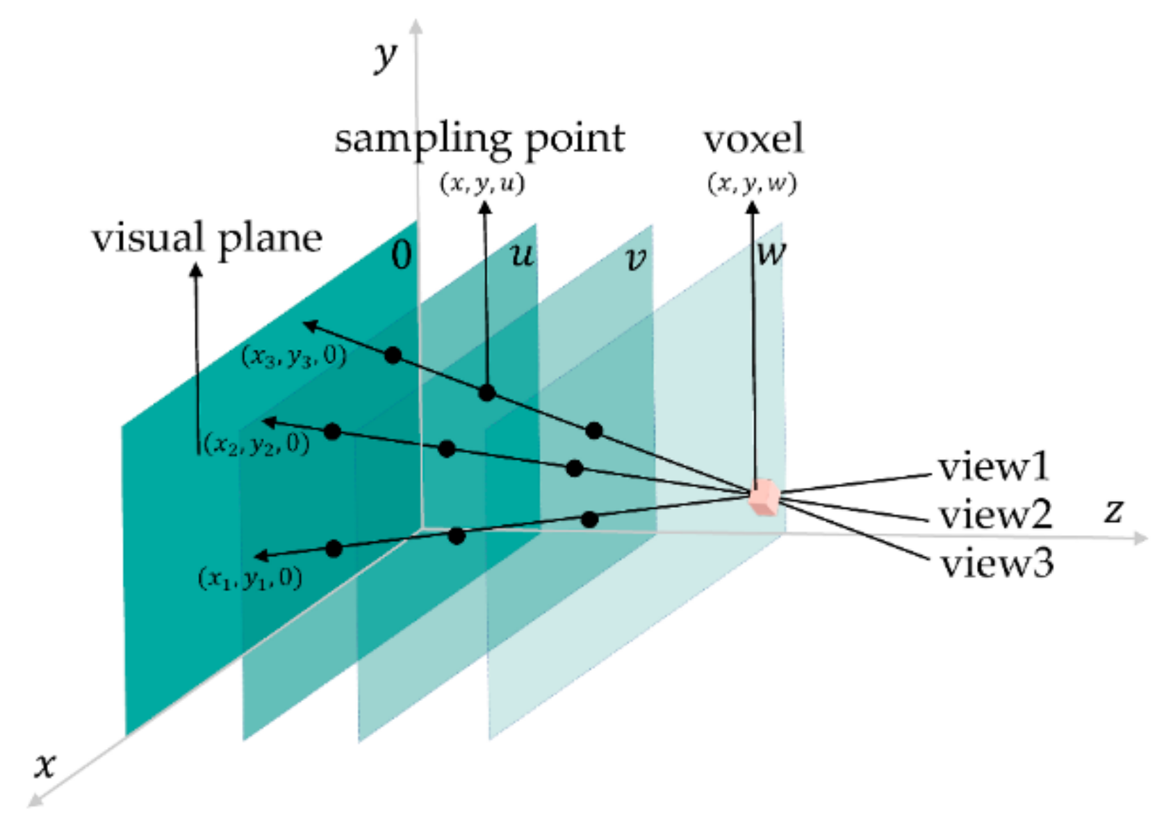
The ray casting algorithm is a kind of volume rendering method. First, it takes the position of the observer as the starting point, and it takes the center of each pixel on the visual plane as the ending point. A ray is emitted along the observation direction and passes through a predefined reconstructed space and splits at equal distance to obtain several sampling point locations with the same interval. Then, the distance between the sampling points of different angles in the same split layer is obtained and an intersection point of rays is determined on the basis of the distance between the sampling points of different ray casting paths in the same split layer. If the distance between the angles of all sampling points is less than the threshold value, then the position of the voxel is determined.
Lastly, the ray casting method achieves 3-D reconstruction of the object by calculating the position of each voxel in the space.
Figure 1 is an illustration of the principle of solving the voxel position by the ray casting algorithm.
The reconstruction method uses a ray casting algorithm to obtain multi-angle parallax information of the sub-satellite point through wide-angle imaging in the orbital direction by using a Directional Polarimetric Camera (DPC) multi-angle sensor. It aims for a 3-D cloud structure reconstruction from 2-D satellite data. In the stereoscopic space, a path from the pixel to the position of the sensor is obtained by observing the zenith angle and the azimuth angle of the pixel during the observation. The path starts from the center of each cloud pixel and ends at the satellite’s position at the same moment. In this case, every angle’s ray casting path between the cloud and satellites is unique for different pixels. Any cloud in the path of 3-D space would cause the starting point of the ray on the 2-D plane to be detected as a cloud. Then, angle information of the cloud pixel of other angles is used to get the path of the angle from the pixels to the location of the sensor. When overlapping of all ray casting paths is located in one position, then this position’s coordinate
of the cloud is considered real.
Figure 2 shows schematic representation of the process.
In a satellite observation process, any significant part of the cloud, unless covered by another clouds group, must be visible from all view angles. In other words, voxel is considered as the cloud voxel if it is crossed by cloud ray casting paths from all angles [
5]. This assumption could eliminate error pixels that falsely determined pixels as cloudy in the cloud binary mask due to a bright surface on the land or sun glint on the sea. Due to limited observation angles of Directional Polarimetric Camera (DPC) data and less resolution, it is expected that this method has rich reconstructed details around the edges of the cloud, but relatively poor details in the central part of the cloud. In addition, the cloud-top height (CTH) may be overestimated in a huge single cloud. Although it is possible to add details of the top of the cloud by a parametric inversion, in this paper, the focus is on the use of DPC data to achieve 3-D reconstruction of clouds based on a multi-angle parallax principle. DPC’s multi-angle information is the kernel of all reconstruction processes.
3. Data and Methods
3.1. Directional Polarimetric Camera (DPC) Data
Directional Polarimetric Camera (DPC), mounted on a GF-5 satellite, is launched on 9 May, 2018 at the Taiyuan satellite launch center of China. It is the only running sensor with observation capability of multi-angle, multi-spectral, and polarization at the same time. It runs in the sun-synchronous orbit whose orbital inclination is 98° with a local overpass time of 13:30 PM and revisiting period of two days. DPC has multi-angle and multi-spectral characteristics with a spatial resolution of 3.3 km × 3.3 km and swath width of 1850 km [
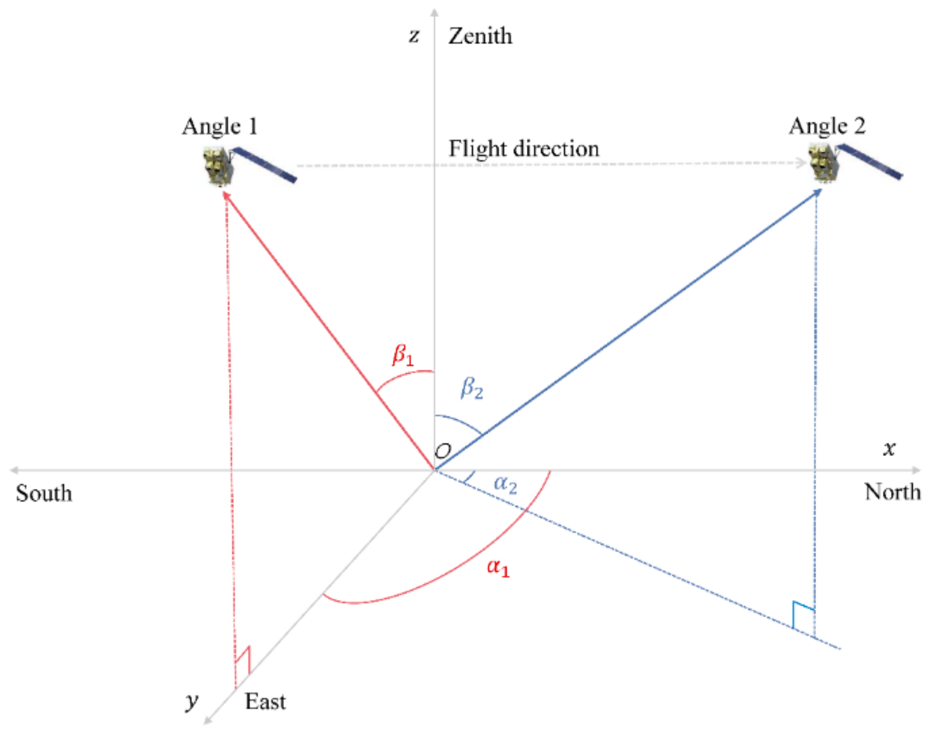
16]. As shown in
Figure 3, in the flight direction, the DPC camera achieved the first image of the target, when the observation zenith angle of the pixel reaches 50°. Every shooting is performed at intervals of 19.51 s, and multi-angle observation information of the same target is acquired by overlapping with the last shooting range. The level 1 data of DPC used in this paper is the product obtained by overlapping the results of different angle observations of each pixel.
3.2. Cloud Mask
Clouds can be detected over land and sea based on the difference in reflectivity of blue and near-infrared bands between clouds and the underlying surface.
Land is mainly covered by many features such as soil, grassland, forests, etc. These surfaces have characteristics with a variation in wavelength, which bring changes in the reflectivity level. In contrast, clouds have stable reflectivity under the conditions of different wavelengths. Cloud pixels and land pixels can be separated based on a difference of 490 nm channel reflectivity. We used a molecular scattering calculation module in the 6SV model to simulate atmospheric molecular scatter value
of each pixel in 490 nm. Real reflectivity of the target is achieved when the measurement value of reflectivity
is subtracted from the atmospheric molecular scatter value
, such as
. According to the method of reference [
17,
18], when real reflectivity is greater than the threshold
, the pixel is detected as a cloud pixel. The sea is mainly covered by water. Therefore, reflectivity of the sea in 865 nm is low, but clouds have high reflectivity. This difference of reflectivity between sea and clouds can help us to detect clouds over the sea. Therefore, we use 865-nm near-infrared band reflectivity from DPC data to detect clouds over the sea. In addition, it is important to avoid the influence of ocean flares. It can be mistakenly recognized as clouds because of high reflectance values. When the flare angle θ is less than 30°, the pixel is considered to be a non-solar flare pixel. For such areas, we also get atmospheric molecular scattering value
by the molecular scattering calculation module in the 6SV model and, to detect clouds pixels by the threshold
as a reference [
17,
18].
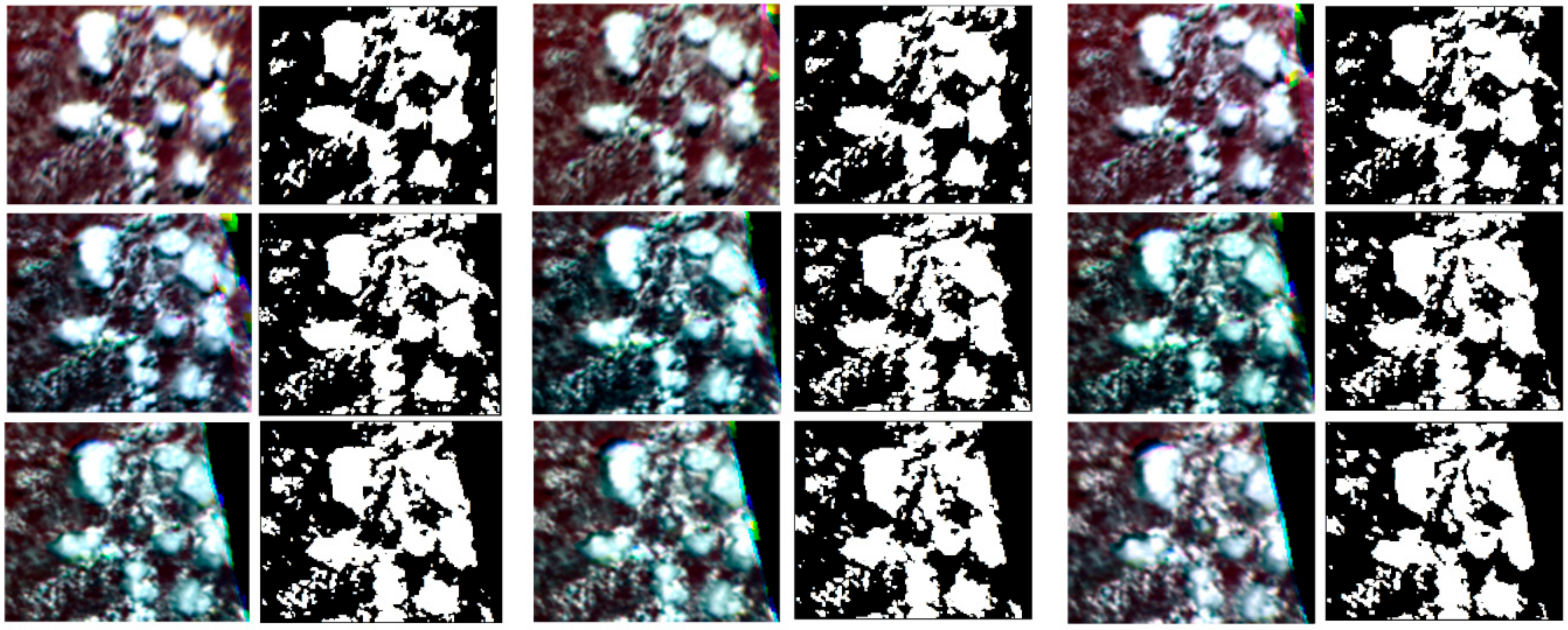
In this case, a cloud binary mask from L1 level data of the DPC can be obtained and channel information of each angle can be used to build all angles’ cloud binary mask. More details on this point can be found in the literature.
As shown in
Figure 4, the selected case covers the central land of Africa. In the Red-Green-Blue (RGB) image, it can be seen that the shape of the cloud is not changed significantly on nine angles, but the position relative to the ground is changed. This feature is more apparent in the cloud binary mask image. The direction of data acquired by the DPC sensor is from the south to the north, which is opposite to the visual trend of cloud’s movement from the north to the south. This difference is consistent with the theory of a multi-angle parallax.
3.3. Ray Casting
The most critical step in cloud structure reconstruction is ray casting. These rays are defined in terms of a cloud binary mask and observed geometric angles. When rays pass through the reconstructed space, the voxels could be defined as either cloud voxels or non-cloud voxels.
In the calculation of the ray casting path of DPC data, positional correspondence between clouds pixels and satellite is included. According to the ray casting theory from literature [
19,
20,
21], we pre-define the reconstruction region, and express a relationship between them in a 3-D local coordinate system with cloud pixels as the coordinate origin. As shown in
Figure 5, in this relationship model, the cloud pixel and satellite’s position are represented by the absorption model and emission model in ray casting, respectively. Ray casting starts from the emission model (cloud pixel center) and ends at the absorption model (satellite camera).
Conical surface equation determined by view of the zenith angle
.
Flat equation determined by the view azimuth angle
.
Result of simultaneous Equation (1) and Equation (2).
During the observation of the satellite, it may acquire the same observation zenith angle in both forward and backward directions with respect to the position of clouds. As shown in
Table 1, this paper determines the emission direction of the ray casting path, according to the range of the observation azimuth angle (α).
As shown in
Table 1, the purpose of defining angles is to limit the range of x and y to ensure that the projection equation is unique.
Clouds generally exist in the atmosphere below an altitude of 20 km. A reasonable scope limitation of the reconstruction area can reduce unnecessary calculations and improve the efficiency of the reconstruction. As shown in
Figure 6, we determine the voxel position through a 3-D Cartesian coordinate system, where the north direction is the X axis, the east direction is the Y axis, the zenith direction is the Z axis, the coordinate origin is
, and the resolution of the stereo space grid is 100 m.
A pre-defined reconstruction area is sliced along the vertical direction every 100 m to obtain 200 slices. It shows that our method is sensitive to the height of clouds, which are greater than 100 m. For each sliced plane, we can find cloud voxels by determining whether rays at each angle intersect in the same location or not. If one voxel in a sliced plane has an intersection point in the range of the distance threshold (DTH), then it is determined as a cloudy voxel. In this case, whether the voxel is cloudy or not, a section in which the ray is passed by the smallest zenith angle is considered to be a coordinate of central point
and other ray passing points
are matching points of the same voxel.
where
is the diagonal distance of the vertices of the pixel. When the distance between the matching point and the center point is less than threshold
, the voxel is considered to be a cloud voxel, and its coordinates in space are recorded.
Voxels of all the solved elevation layers are expressed in the same reconstruction area as shown in
Figure 7.
4. Results
Two sample areas are selected from the orbit of 1044 and 1050 on 27 May 2018. The result presented in this section shows different reconstructed cloud structures above the land and ocean surface from DPC data. We choose a vertically developed cluster of clouds with prominent edges. Those clouds almost have a better reconstructed effect. The reason for choosing these samples is that elevations of these clouds have different characteristics. Elevation of the cloud in sample 1 is about 10 km while, in sample 2, it is about 2 km. In different cloud elevations, parallax information of the ray casting path is different, which would have a great impact on the calculated result of the ray casting equation. A 3-D cloud reconstruction algorithm explored in this paper takes into account the differences caused by different cloud elevations, and it has a good reconstruction effect for clouds at different altitudes. In addition, the two sample areas have cloudy overlaps at the edges of clouds. These subtle edge features are difficult to capture in traditional single-angle remote sensing, but this difference is revealed through multi-angle 3-D cloud reconstruction easily. The two selected samples have similar edge overlap reconstructions to highlight advantages and characteristics of the algorithm.
Due to a lack of data from synchronous active remote sensing products, verification of cloud 3-D reconstruction results is a challenge. However, the Cloud-Aerosol Lidar with Orthogonal Polarization (CALIOP) can obtain vertical profile information of the atmospheric composition along the track, such as aerosol, cloud, air, etc. The cloud is one of the crucial ingredients of a Vertical Feature Mask (VFM) of CALIOP. In both samples, the CALIOP data with a similar overlapped area and observation time is selected and compared with the section of reconstructed results.
4.1. Oribit 1044
The sample 1 chosen for reconstruction is located in the desert of the outback in Australia. This orbit is observed from 04:33:21 to 05:19:08 UTC on 2 May 2018.
Figure 8 shows an overlaying image of RGB and cloud binary mask of different views.
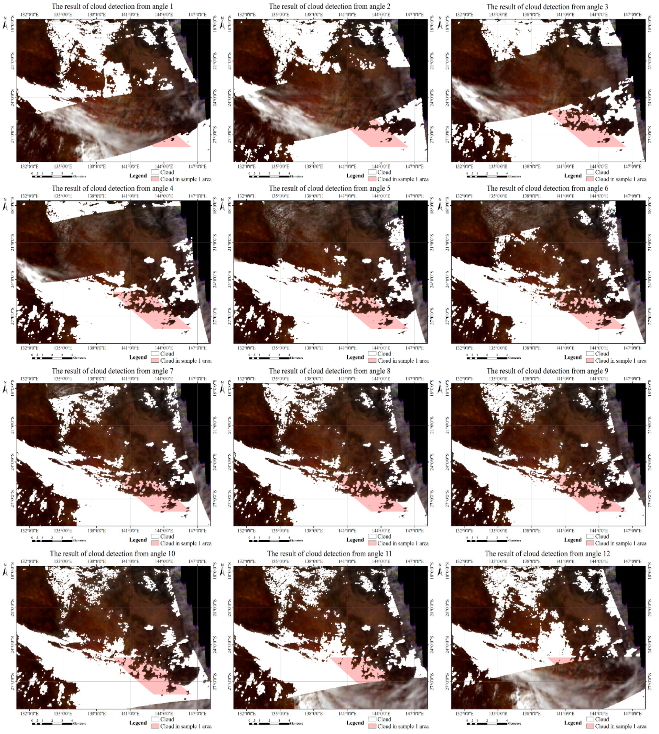
Table 2 shows the coverage of valid value and cloud for different views. Different views of observation lead to different coverage areas. In sample 1, as shown in
Table 2, the coverage of the valid value from angle 3 to angle 10 is above 99.9%, but the coverage from other views is relatively low, between 11.25% and 63.95%. This indicates that a valid value of coverage from different angles has a great difference. There are significant differences in cloud detection results from different views. We compare the angles from 3th to 10th. The maximum rate of cloud coverage is 60.71% and the minimum is 36.61%. This difference shows that parallax at different views is clear in the cloud mask. In the northwestern part of the sample 1 area, there are significant differences in the results of cloud detection at different angles because this area is mainly occupied by broken thin clouds. In the southwestern part, consistency of different angle’s cloud pixel location is higher. Non-obvious parallax information among thicker and larger clouds are the main reasons. Along with the changes in different angles, other areas also show different cloud detection results.
In
Figure 9, the sample area is completely covered by observed pixels from angle 3 to 10, and the ray casting paths of each angle are from the center of the recognition of the cloud pixel to the simultaneous entrance of the satellite. From the direction of integration of the ray casting path, the zenith of angle 5 is closest to 0°. Azimuth of the angles 3 and 10 are biased toward south and north to constitute front and rear views in a multi-angle shooting, respectively. Azimuth of the remaining observations is a regular change from the southerly direction to the northerly direction. Since angle 5 is close to the zenith direction, it is clear that layering information between clouds is largely obscured in the northeast corner of the ray casting path integration results. For angle 10, its layering is clearer because information of the cloud acquired from different observation angles is different. Oblique angle captures are found rich with information about the edges of clouds.
In
Figure 10, 3-D the cloud reconstruction result is calculated by the distance threshold (DTH), according to the ray casting path of angles 3 to 10, shown in
Figure 9. Some discrete clouds disappear in the northern part, but they can be found in individual angle’s ray casting path because clouds that are only visible at a partial angle are omitted from the reconstruction results. In the southern edge of sample 1, due to a lack of the partial angle’s cloud observation information, a reconstructed cloud structure is skewed. The reason is that a different sampling range is selected according to the latitudes and longitudes, since observation information of some angles are outside the range of sample 1. The northern part of the 3-D reconstructed cloud is mainly composed of small broken clouds, and the algorithm has achieved super reconstruction effects in this area. Texture information of the cloud in all directions is accurately characterized, which is in good agreement with the shape in the Red-Green-Blue (RGB) image. This illustrates advantages of the method for small clouds reconstruction. The southern part of the cloud 3-D reconstruction results consists of a whole piece of contiguous cloud. At the boundary of the cloud around the non-edge of the sample 1 area, results of cloud reconstruction have abundant details. It has a good consistency with the visual perception in RGB images to show that this method has a good reconstruction effect on the edges of large clouds.
As shown in
Figure 11 the Moderate Resolution Imaging Spectroradiometer (MODIS) data that is synchronously observed with the CALIOP as the RGB color base map is selected. According to the position of the cloud on the track of CALIOP and the RGB image of Moderate Resolution Imaging Spectroradiometer (MODIS), the position of the 3-D cloud slice is determined in
Figure 11b. The position of the slice in
Figure 11b is determined by texture and the current state of the cloud in
Figure 11a. Additionally, as far as possible, the position of the slice of a reconstructed cloud is similar to the orbit of the CALIOP relative to the cloud. Then, we can find out whether results of 3-D cloud reconstruction are accurate or not by comparing it with the altitude and trend of changes in the cloud through Vertical Feature Mask (VFM). The comparison of CALIOP and 3-D cloud reconstruction are obtained by a minimum distance of latitudes and longitudes. The latitudes and longitudes from DPC data are shown in
Figure 11c.
Figure 11c is a comparison between
Figure 11a,b.
Figure 11a is a cloud information of VFM in the blue line position and
Figure 11b shows extraction results of a 3-D reconstructed cloud profile in a red line. In this scenario, the contrast area will be described from A to E. In the dashed box A, CTH of the reconstructed cloud is consistent with the altitude of VFM’s cloud, at about 2.5 km. In the dashed box B, a small double-layer structure is captured at the top of the cloud. In traditional passive optical remote sensing, detection of a double-layer cloud is difficult in a fixed observation angle, but multi-angle cloud remote sensing can solve this problem and express it in the form of a 3-D structure. In the lower right corner of a dashed box B, the cloud-top height (CTH) at the edge of the cloud and altitude of VFM’s cloud are also consistent for about 2.5 km. In the dashed box C, the profile of 3-D cloud reconstruction is consistent with cloud shape in VFM, which shows a ’step’ shape, and CTH on the right side of the cloud is approximately 11.25 km. In the dashed box D, it is occupied by a bulky whole piece of cloud. The overestimation of the middle part of the cloud cluster is marked with pale pink in
Figure 11. The overestimation of CTH is caused by insufficient parallax information of the cloud cluster. An increasing observation angle of the instrument or resolution of the sampling can eliminate errors. On the other hand, the algorithm has a good reconstruction effect for small clouds, especially in the edges of a cloud. In the dashed box E, an apparent multi-layer cloud overlap is expressed in 3-D cloud reconstruction by the algorithm in this paper. This accurate depiction of the cloud edge of a multi-layer cloud superimposed area is the main feature of the algorithm. In addition, the left cloud in the E-dashed box still has an overestimation of cloud-top height (CTH).
As shown in
Table 3, according to the track of CALIOP, a total of 116 sampling points is collected. We classify differences between the height of 3-D cloud and clay products of CALIOP. The difference is calculated every 100 m from 0.1 km to 1 km. In 10 intervals, we can get the number of sample points that satisfy the condition. As shown in
Table 3, since two overestimations of cloud tops of dashed box D and E are included, the accuracy is only 74.14% within 1 km, but the precision reaches 62.93% within 100 m. Overestimation of CTH has a significant impact on overall precision. This overestimation will be solved in future work.
4.2. Oribit 1050
The second sample is selected over the Atlantic Ocean near Western Africa. The orbital shooting starts at 14:26:26, and ends at 15:12:12 UTC.
Cloud detection of different angles is shown in
Figure 12 and
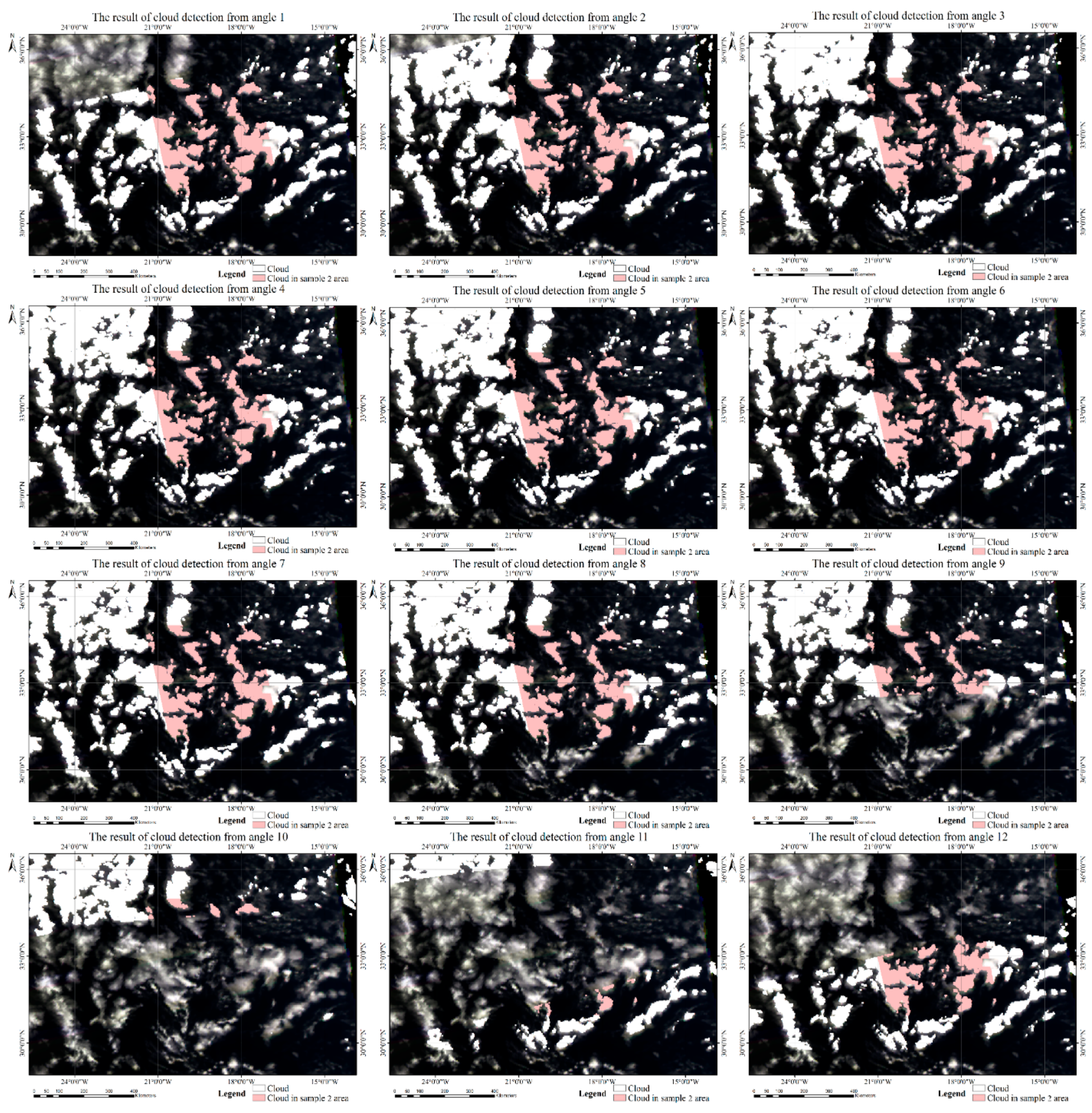
Table 4. Coverage of a valid value in angle 1~8 cover the target area above 99.20%, but angle 9–12 are not fully covered, which range from 15.33% to 62.24%. Coverage of cloud mask ranges from 22.81% to 27.49% between angle 1 and angle 8. Because the height of sample 2’s cloud is lower than sample 1, the parallax of cloud mask becomes significantly smaller. Judging from the RGB base image, sample 2 is mainly occupied by discrete clouds, rather than continuous large clouds. Among clouds in the northwest corner of sample 2, from angles 1 to 12, these are judged as a cloud group or two independent clouds. Compared with the RGB image, it is inferred that there is a lower stratus or fog, which leads to the difference in cloud detection results at different angles. This difference between different angles is useful for eliminating the interference of non-cloud pixels on 3-D cloud reconstruction. From angle 1 to 12, the gap between two independent clouds is increased in the southeast corner of sample 2. This phenomenon shows that relative positions between clouds are different under different observation angles. In other words, in a single perspective, it is easy to misjudge the position and shape of the cloud. Correspondingly, multi-angle parallax can help us to avoid this misjudgment.
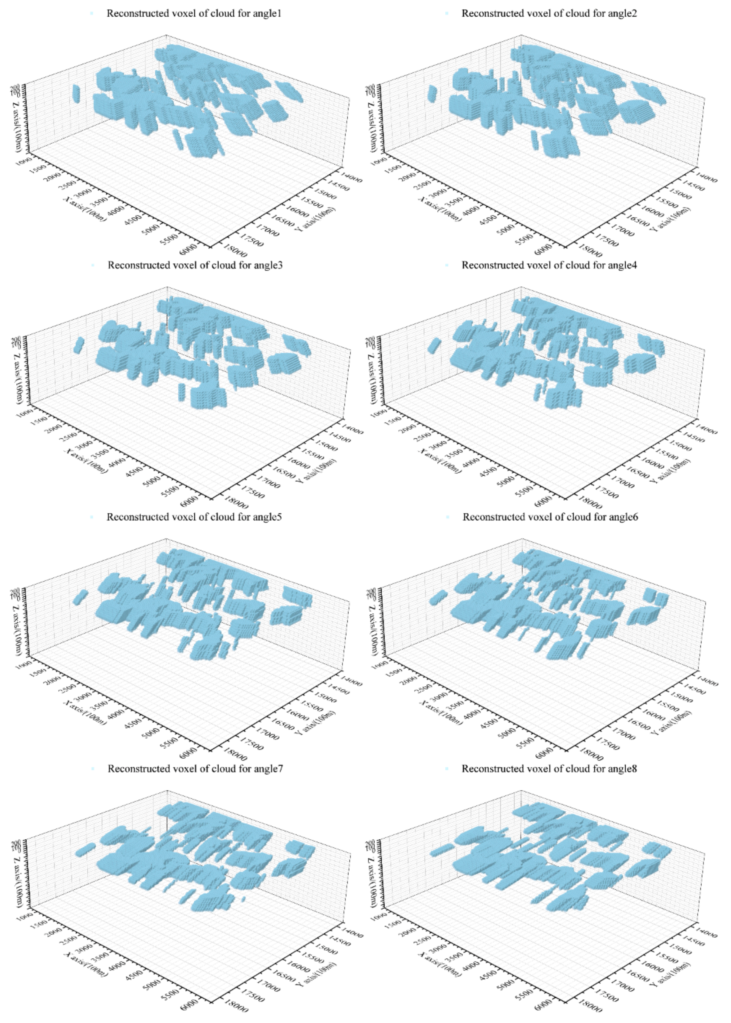
Figure 13 shows ray casting path of all observation angles, the zenith of angle 3 is closest to 0 degrees. Azimuth of angles 1 and 8 are biased toward the south and north to constitute the front and rear views in multi-angle shooting, respectively. Overlapping in multiple-layer clouds in a single direction is difficult to find, but multi-angle observation can find more overlapping information through parallax. For example, the direction of the observation and positions of overlapping pixels of the clouds are nearly in one straight line in angle 3. This overlapping structure can be observed in angle 8. This difference reflects advantages of multi-angle parallax. The cloud in the northeast corner is a whole piece of cloud in angle 3, but the ray casting paths of this cloud are shown to be separated in angle 8. It can be understood that as the degree to which the clouds cover each other is different in different angles. In angle 3, these overlap each other, but, in angle 8, the gap between clouds can be observed clearly. These observation differences of pixels between each angle would play a role in the reconstruction of the 3-D cloud.
In
Figure 14, the 3-D cloud reconstruction result is calculated by the distance threshold (DTH), according to the ray casting path of angles 1 to 8. In the RGB image, many small clouds can be seen with different altitudes and different volumes in the sample 2 area. For example, even if height and shape of small clouds are significantly different in sample 2, reconstruction of it in the southern region is possible with greater accuracy. In addition, the phenomenon of cutting edges is not clear in sample 2 in comparison with sample 1 because it is mainly composed of small scattered clouds at the edges. In different angle’s observation, the number of completely non-shown edges of clouds decreases. There is only a slight tilt effect on the west side of the case area due to small clouds. Compared with the shapes of clouds in the RGB image, the reconstructed cloud has a similar appearance. In the RGB image, the edges of clouds characterize variation in thickness of the cloud in terms of depth in color. In the reconstructed model, the shape of the boundary of different thick clouds is also shown to be accurate. In comparison with sample 1, the reconstruction area is much smaller, and a smaller domain puts forward new requirements for the degree of refinement of 3-D cloud reconstruction. Thickness differences of the clouds and accuracy of the shapes of the edges are particularly important. The algorithm can meet new accuracy requirements for reconstruction of the cloud edges in this paper. The cloud in the reconstruction area has a low altitude, at about 2 km, which belongs to the mix area of the cloud and fog. Mixing of clouds can affect the accuracy of cloud detection and even affect the effect of 3-D cloud reconstruction. A lower height of clouds creates difficulty for different angles of observations in the positions of clouds. This variety would reduce the parallax information and increase difficulty of 3-D cloud reconstruction. However, the method still has a good reconstruction effect for a cluster of clouds for about 2 km. The higher the cluster of clouds, the richer the parallax information will be for a better reconstruction effect. This indicates that the method has a good reconstruction effect on clusters of clouds within the range of height of the main clouds’ distribution.
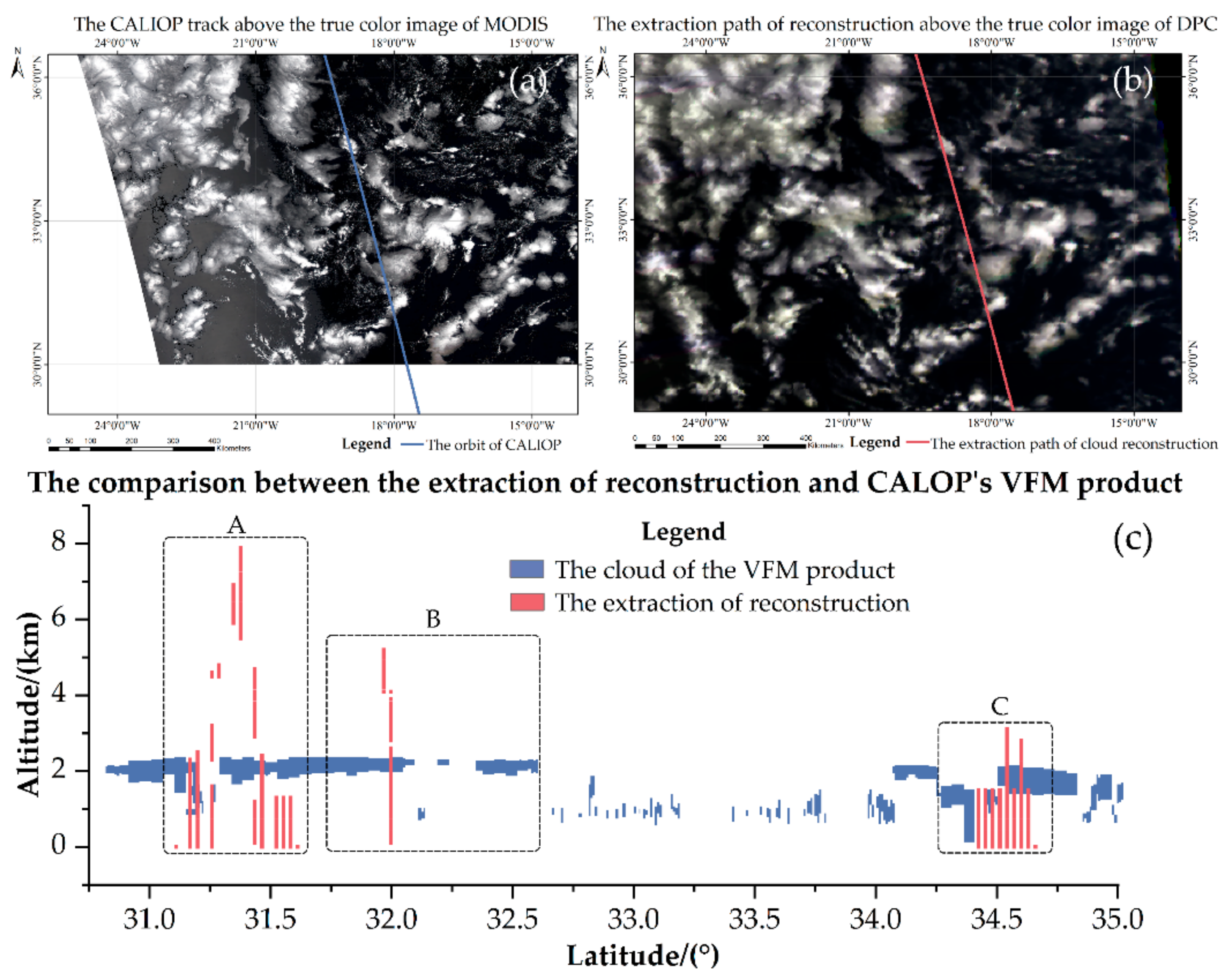
Figure 15 shows a comparison between 3-D cloud reconstruction and the cloud of the VFM corresponding to sample 2. In this case, the contrast area is described from A to C for sample 2.
In the dashed box A, the reconstructed 3-D cloud contains two main parts. In sample 2, there is consistency in the shape of the cloud on its left part with the cloud of VFM. Their distance threshold (CTH) are approximately 2 km. The right part is slightly lower than the VFM. A broken cloud cluster with a higher altitude appears in the center of dashed box A. Referring to
Figure 16, information about clouds at a high altitude is actually extracted from the cloud pixel of the adjacent track. In this case, the threshold of latitudes and longitudes is used to extract alongside track pixels. Resolution of the DPC pixel is 3.3 km × 3.3 km. This low resolution causes elevation of pixels to be extracted from non-tracks. In this sample, it is reflected that altitude is too high in some positions. In the dashed box B, information extracted from 3-D clouds is less, while the Vertical Feature Mask (VFM) has recorded more information about clouds. By comparing the results of the clouds detection in
Figure 12, it is found that the cloud cluster in this area is thin due to interference from the underlying surface. It is misjudged as a non-cloud pixel, which results in non-3-D cloud reconstruction in this area. In reconstructed results, abnormal spectral information of the surface will cause a pixel to be incorrectly detected as a non-cloud pixel. This shows that accuracy of cloud detection can impact 3-D cloud reconstruction results of this algorithm. In the dashed box B, there is also an abnormal protrusion, which is similar to the case in the center of dashed box B, and it is also affected by the resolution of the Directional Polarimetric Camera (DPC) pixel. This phenomenon is also shown in a 3-D space in
Figure 16. Within the dashed box of C, it is an independent cloud located at the north of the case area. The morphological structure of the cloud is concave. Using a comparison between the extracted shape of the 3-D cloud and the cloud of Vertical Feature Mask (VFM), we find that cloud-top height (CTH) is consistent, and the height of the bottom of the cloud is about 1.6 km. The results of 3-D reconstruction have a good expression of the shape and characterization of the cloud.
As shown in
Table 5, we use the same quantitative verification method with sample 1. Since sample 2 has only 30 sampling points, overvaluation of the cloud top in dashed box A and B has a large impact on the verification results. We separately counted the clouds in the dashed box C. As shown in
Table 4, it is found that, when the precision is 0–0.2 km, the sampling accuracy of dashed box C has reached 90.91%. This result indicates good accuracy of our method.
5. Discussion and Conclusions
The main aim of this paper is building a 3-D cloud structure reconstruction from Directional Polarimetric Camera (DPC) data using a ray casting method. First, cloud detections are conducted with 490 nm and 865 nm for every angle to find differences between different angles. Then, based on such results of each angle, a binarized cloud mask of each angle is constructed separately. According to information from the observation of geometric angles of cloud pixels in a binarized cloud mask, an integral of the ray casting the path of the satellite’s position of observation to the cloud pixel is calculated. In this way, integration results of each angle along directions of observation can be obtained. Lastly, according to the slice by the altitude, distance threshold (DTH) is used to determine the position of the cloud voxel in the same plane of altitude. All cloud voxels are visually expressed to obtain the voxel form of the cloud in a 3-D space.
Currently, there are few studies on the 3-D cloud reconstruction based on geometric information of multi-angle images. In one of the research studies, this principle is applied on the Multi-angle Imaging SpectroRadiometer (MISR) data. However, imaging width of DPC is 1850 km while imaging width of MISR is 380 km. Directional Polarimetric Camera (DPC) can achieve higher coverage than MISR in one track. With the help of DPC data, 3-D clouds reconstruction is possible for the clouds of thousands of kilometers of size. Such results would provide basic data for inversion of property of a 3-D cloud, which will be beneficial for us to explore the impact of clouds on atmospheric conditions. For example, the reconstruction of the 3-D structure of typhoon and inversion of its property are very meaningful. The diameter of typhoon can reach hundreds or even thousands of kilometers, and the width of MISR’s imaging cannot satisfy entire 3-D cloud reconstruction of the typhoon. In addition, the rich channels of DPC also includes three polarization channels. Therefore, compared with the MISR data, the 3D cloud reconstruction method based on DPC data has more advantages. Considering the characteristics of DPC data, results of cloud reconstruction are shown for two hand-picked scenes, where one is within Orbit 1044 and another is within Orbit 1050.
Trends in results of reconstruction are considered similar to the Vertical Feature Mask (VFM) of CALIOP data. The method uses DPC data to rebuild the 3-D cloud, which not only enriches the application field of the data but also improves utilization efficiency of the data. Yet, the results of 3-D cloud reconstruction are visually positive and accurate with products of CALIOP. We also need to note several limitations.
In comparison with the active sensor, CALIOP is an active optical device with the closest time observation, but it also has a difference with DPC. Shape and location of the cloud changes very quickly. Ground-based and airborne instruments can provide a reliable synchronous observation of cloud structure estimation [
22,
23,
24,
25,
26]. In the future, we can select appropriate ground-based instruments to evaluate reconstruction of 3-D clouds [
27,
28].
The reconstructed edge of the 3-D cloud is accurate, but CTH is overestimated due to little difference in multi-angle information in the central area of a large homogeneous cloud. If we can get information from observation of other instruments carried on the GF-5, a rich multi-angle parallax information would help improve reconstruction of a 3-D cloud near the central area.
Influence of winds on 3-D reconstruction is not considered comprehensive in our method. According to the size of the DPC pixel, we believe that, when speed of winds is faster than 19 m/s, it may affect the accuracy of 3-D reconstruction. For such errors, data of wind speeds from simultaneous observations is necessary for a correction. In the future with appearance of wind speed products of GF-5 data, accuracy in reconstruction can be improved.
Under current technical conditions, breaking through the above restrictions, improvement of the algorithm requires plenty of work. Despite these limitations, a 3-D cloud reconstructed by the ray casting method has clear advantages, and these advantages have a great impetus on cloud research.
Inversion of boundary features of clouds have always been a difficult point in cloud-related research. In this region, clouds, aerosols, and other atmospheric components interact and makes the parameter inversion of the boundary uncertain when compared to the central region. This is a major difficulty in the inversion of cloud parameters. 3-D cloud reconstruction based on the ray casting method has higher accuracy in shapes and boundary of clouds, which can help improve deficiencies in traditional methods. It provides an explanation for the situation of different cloud features, which also improves the accuracy of calculations of microphysical parameters and optical properties of clouds.
Directional Polarimetric Camera (DPC) is a sun-synchronous orbit satellite with a stable revisit cycle feature. It provides a long-term observation for studying 3-D reconstruction of clouds in a particular region. At the same time, it provides accuracy of calculation of 3-D radiation transmission in a cloudy atmosphere, which would greatly help study the influence of 3-D clouds on Earth’s radiation balance, and even to study evolution of extreme weather and processes related to it.
Spatial voxelization form of the 3-D cloud constructed in this paper is equivalent to an unfilled 3-D database. Each of the voxels can be filled with attributes, and all voxels can be carriers of 3-D cloud parameters. In future work, 3-D representation of various cloud attributes would be achieved by populating this database.
In the process of constructing a 3-D cloud, the main technical difficulties have a lower DPC resolution, small observation difference in all angles, and a lack of synchronous observation data. By improving the resolution and difference in all angles of the instrument, the information of multi-angle parallax can greatly increase. This will alternately improve the 3-D reconstruction effect of the cloud. In addition, due to a lack of active radar for quasi-synchronous observations, it is actually difficult to quantify the accuracy of 3-D cloud reconstruction. If a synchronous observation of active radar and a DPC multi-angle sensor is possible, then mutual observation of two instruments can be achieved. In this way, 3-D cloud reconstruction might gain a larger range and higher precision.
Author Contributions
Conceptualization, H.Y. and J.M. Methodology, H.Y. and J.M. Software, H.Y. Validation, H.Y. and J.M. Formal analysis, H.Y. and J.M. Investigation, H.Y. and J.M. Resources, H.Y. and J.M. Data curation, H.Y., E.S., and C.L. Writing—Original draft preparation, H.Y. Writing—Review and editing, H.Y., S.A., and J.M. Visualization, H.Y. and J.M. Supervision, J.M., Z.L., and J.H. Project administration, J.M. Funding acquisition, none. All authors read the manuscript, contributed to the discussion, and gave valuable suggestions to improve the manuscript.
Funding
The National Natural Science Foundation of China (Grant No. 41671352), the university academically funded projects (gxbjZD06), and the K. C. Wong Education Foundation (GJTD-2018-15) funded this research.
Acknowledgments
The GF-5 DPC data used in this paper are provided by the China Centre for Resources Satellite Data and Application (CRESDA) and the Anhui Institute of Optics and Fine Mechanics (AIOFM). The MODIS and CALIPSO data are obtained from the ICARE Data and Services Center (
http://www.icare.univ-lille1.fr/). We thank the DPC, MODIS, and CALIPSO team for the data used in our research.
Conflicts of Interest
The authors declare no conflicts of interest.
References
- Arakawa, A. Modelling clouds and cloud processes for use in climate models. In The Physical Basis of Climate and Climate Modelling; SEE N 76-19675 10-47; WMO: Geneva, Switzerland, 1975; pp. 183–197. [Google Scholar]
- Wielicki, B.A.; Cess, R.D.; King, M.D.; Randall, D.A.; Harrison, E.F. Mission to planet Earth: Role of clouds and radiation in climate. Bull. Am. Meteorol. Soc. 1995, 76, 2125–2154. [Google Scholar] [CrossRef]
- Cess, R.D.; Potter, G.; Blanchet, J.; Boer, G.; Del Genio, A.; Deque, M.; Dymnikov, V.; Galin, V.; Gates, W.; Ghan, S. Intercomparison and interpretation of climate feedback processes in 19 atmospheric general circulation models. J. Geophys. Res. Atmos. 1990, 95, 16601–16615. [Google Scholar] [CrossRef]
- Barker, H.; Jerg, M.; Wehr, T.; Kato, S.; Donovan, D.; Hogan, R.J.Q.J.o.t.R.M.S. A 3D cloud-construction algorithm for the EarthCARE satellite mission. Q. J. R. Meteorol. Soc. 2011, 137, 1042–1058. [Google Scholar] [CrossRef] [Green Version]
- Lee, B. Three-Dimensional Cloud Volume Reconstruction from the Multi-Angle Imaging SpectroRadiometer. Available online: http://hdl.handle.net/2142/99363 (accessed on 30 April 2019).
- Diner, D.J.; Beckert, J.C.; Reilly, T.H.; Bruegge, C.J.; Conel, J.E.; Kahn, R.A.; Martonchik, J.V.; Ackerman, T.P.; Davies, R.; Gerstl, S.A. Multi-angle Imaging SpectroRadiometer (MISR) instrument description and experiment overview. IEEE Trans. Geosci. Remote Sens. 1998, 36, 1072–1087. [Google Scholar] [CrossRef]
- Lee, B.; Di Girolamo, L.; Zhao, G.; Zhan, Y.J.R.S. Three-Dimensional Cloud Volume Reconstruction from the Multi-Angle Imaging SpectroRadiometer. Remote Sens. 2018, 10, 1858. [Google Scholar] [CrossRef] [Green Version]
- Li, X.; Zheng, X.; Zhang, D.; Zhang, W.; Wang, F.; Deng, Y.; Zhu, W.J.A. Clouds over East Asia Observed with Collocated CloudSat and CALIPSO Measurements: Occurrence and Macrophysical Properties. Atmosphere 2018, 9, 168. [Google Scholar] [CrossRef] [Green Version]
- Desmons, M.; Ferlay, N.; Parol, F.; Riédi, J.; Thieuleux, F. A global multilayer cloud identification with POLDER/PARASOL. J. Appl. Meteorol. Climatol. 2017, 56, 1121–1139. [Google Scholar] [CrossRef]
- Sinclair, K.; Diedenhoven, B.V.; Cairns, B.; Yorks, J.; Wasilewski, A.; McGill, M. Remote sensing of multiple cloud layer heights using multi-angular measurements. Atmos. Meas. Tech. 2017, 10, 2361–2375. [Google Scholar] [CrossRef] [Green Version]
- Heinzleiter, P.; Kurka, G.; Volkert, J. Real-time visualization of clouds. In Proceedings of the 10th International Conference in Central Europe on Computer Graphics, Visualization and Computer Vision, Pilsen, Czech Republic, 4–8 February 2002; pp. 43–50. [Google Scholar]
- Nouri, B.; Kuhn, P.; Wilbert, S.; Prahl, C.; Pitz-Paal, R.; Blanc, P.; Schmidt, T.; Yasser, Z.; Santigosa, L.R.; Heineman, D. Nowcasting of DNI maps for the solar field based on voxel carving and individual 3D cloud objects from all sky images. In AIP Conference Proceedings; AIP Publishing: Melville, NY, USA, 2018; p. 190011. [Google Scholar]
- Xu, F.; Ma, J.; Wu, S.; Li, Z.; Transfer, R. Identification of smoke and polluted clouds based on polarized satellite images. J. Quant. Spectrosc. Radiat. Transf. 2019, 224, 343–354. [Google Scholar] [CrossRef]
- Várnai, T.; Marshak, A.J.A. Satellite Observations of Cloud-Related Variations in Aerosol Properties. Atmosphere 2018, 9, 430. [Google Scholar] [CrossRef] [Green Version]
- Ching, J.; Zaveri, R.A.; Easter, R.C.; Riemer, N.; Fast, J.D. A three-dimensional sectional representation of aerosol mixing state for simulating optical properties and cloud condensation nuclei. J. Geophys. Res. Atmos. 2016, 121, 5912–5929. [Google Scholar] [CrossRef] [Green Version]
- Li, Z.; Hou, W.; Hong, J.; Zheng, F.; Luo, D.; Wang, J.; Gu, X.; Qiao, Y.J.; Transfer, R. Directional Polarimetric Camera (DPC): Monitoring aerosol spectral optical properties over land from satellite observation. J. Quant. Spectrosc. Radiat. Transf. 2018, 218, 21–37. [Google Scholar] [CrossRef]
- Ackerman, S.; Holz, R.; Frey, R.; Eloranta, E.; Maddux, B.; McGill, M.J.; Technology, O. Cloud detection with MODIS. Part II: Validation. J. Atmos. Ocean. Technol. 2008, 25, 1073–1086. [Google Scholar] [CrossRef] [Green Version]
- Li, C.; Ma, J.; Yang, P.; Li, Z.J.; Transfer, R. Detection of cloud cover using dynamic thresholds and radiative transfer models from the polarization satellite image. J. Quant. Spectrosc. Radiat. Transf. 2019, 222, 196–214. [Google Scholar] [CrossRef]
- Haines, E.A.; Wallace, J.R. Shaft culling for efficient ray-cast radiosity. In Photorealistic Rendering in Computer Graphics; Springer: Berlin/Heidelberg, Germany, 1994; pp. 122–138. [Google Scholar]
- Roth, S. Ray casting for modeling solids. Comput. Graph. Image Process. 1982, 18, 109–144. [Google Scholar] [CrossRef]
- Levoy, M. A hybrid ray tracer for rendering polygon and volume data. IEEE Comput. Graph. Appl. 1990, 10, 33–40. [Google Scholar] [CrossRef]
- Fielding, M.D.; Chiu, J.C.; Hogan, R.J.; Feingold, G. A novel ensemble method for retrieving properties of warm cloud in 3-D using ground-based scanning radar and zenith radiances. J. Geophys. Res. Atmos. 2014, 119, 10912–10930. [Google Scholar] [CrossRef] [Green Version]
- Zinner, T.; Mayer, B.; Schröder, M. Determination of three-dimensional cloud structures from high-resolution radiance data. J. Geophys. Res. Atmos. 2006, 111. [Google Scholar] [CrossRef]
- Beekmans, C.; Schneider, J.; Läbe, T.; Lennefer, M.; Stachniss, C.; Simmer, C. Cloud photogrammetry with dense stereo for fisheye cameras. Atmos. Chem. Phys. 2016, 16, 14231–14248. [Google Scholar] [CrossRef] [Green Version]
- Zinner, T.; Schwarz, U.; Kölling, T.; Ewald, F.; Jäkel, E.; Mayer, B.; Wendisch, M. Cloud geometry from oxygen-A-band observations through an aircraft side window. Atmos. Meas. Tech. 2019, 12, 1167–1181. [Google Scholar] [CrossRef] [Green Version]
- Alexandrov, M.D.; Cairns, B.; Emde, C.; Ackerman, A.S.; Ottaviani, M.; Wasilewski, A.P. Derivation of cumulus cloud dimensions and shape from the airborne measurements by the Research Scanning Polarimeter. Remote Sens. Environ. 2016, 177, 144–152. [Google Scholar] [CrossRef]
- Campbell, J.R.; Vaughan, M.A.; Oo, M.; Holz, R.E.; Welton, E.J. Distinguishing cirrus cloud presence in autonomous lidar measurements. Atmos. Meas. Tech. 2014, 8, 435–449. [Google Scholar] [CrossRef] [Green Version]
- Lewis, J.R.; Campbell, J.R.; Welton, E.J.; Stewart, S.A.; Haftings, P.C. Overview of MPLNET, Version 3, Cloud Detection. J. Atmos. Ocean. Technol. 2016, 33, 2113–2134. [Google Scholar] [CrossRef]
Figure 1.
Principle of ray casting in 3-D reconstruction. The reconstructed space is determined by an x- y-z coordinate system, and is equally sliced to obtain a sampling plane of z = 0, u, v, and w. The pink cube is the target of observation. In this case, the pink cube is observed along the directions of view 1, view 2, and view 3. The rays are passed through the reconstruction area and are sampled on visual planes. As shown in view 3, the sampling point on the u plane is
and the projection point on the visual plane is . Similarly, the projection positions of view 1 and view 2 on the voxel are, respectively, , . Lastly, based on the intersection of the three rays, the intersection of the voxel is determined on the w plane, and the position in the reconstruction space is
Figure 2.
The observation process of ray casting for a multi-angle spaceborne sensor. Red lines are the rays of view 1’s observation. Blue lines are the rays of view n’s observation. View 1 and view n observe the same cloud pixel from different angles, and the obtained pixel positions are different. By calculating the intersection of the ray casting paths of view 1 and view n, a true position of the cloud pixel can be obtained. The range of n is from 1 to 12.
Figure 3.
Process of multi-angle shooting of Directional Polarimetric Camera (DPC) along the track. By taking measurements with nine viewing angles as an example, the DPC sensor sequentially shoots the same target in the track to obtain multi-angle information, which contains data of eight spectral channels. According to comprehensive spectral information and observation angle, DPC can achieve up to 126 measurements per pixel [
16].
Figure 4.
From top left to the bottom right: Red-Green-Blue (RGB) image (left) and cloud binary mask (right) of DPC’s nine angles in the example of central Africa. The angular order is arranged according to the order of the DPC’s Hierarchical Data Format’s (HDF) multi-angle data layers. The positional change of cloud relative to the ground can be seen in each observation angle of the RGB image. In the cloud binary mask, the white part is the detected cloud pixel and the black part is the clear sky pixel.
Figure 5.
Illustration of the observed position between the cloud and satellite.
is the cloud’s position. and are the view azimuth angle of the cloud pixel. and are the view zenith angle of the cloud pixel. A positive direction of the x-axis and y-axis is consistent with the direction of North and East, respectively. A positive direction of the z-axis is consistent with the direction of the zenith. Red and blue lines show paths between the satellite and cloud in two different positions.
Figure 6.
These images are the results of integration on the paths of angle 1–9 ’s voxel. Northward direction is the X-axis, and the east direction is the Y-axis. The normal vector perpendicular to the tangent plane of the earth’s ellipsoid is the Z-axis. In the small span area, it is assumed that the intersection of the cloud and ground in a vertical direction is collinear with this intersection and the center of the earth, so the Z-axis can be considered as the altitude.
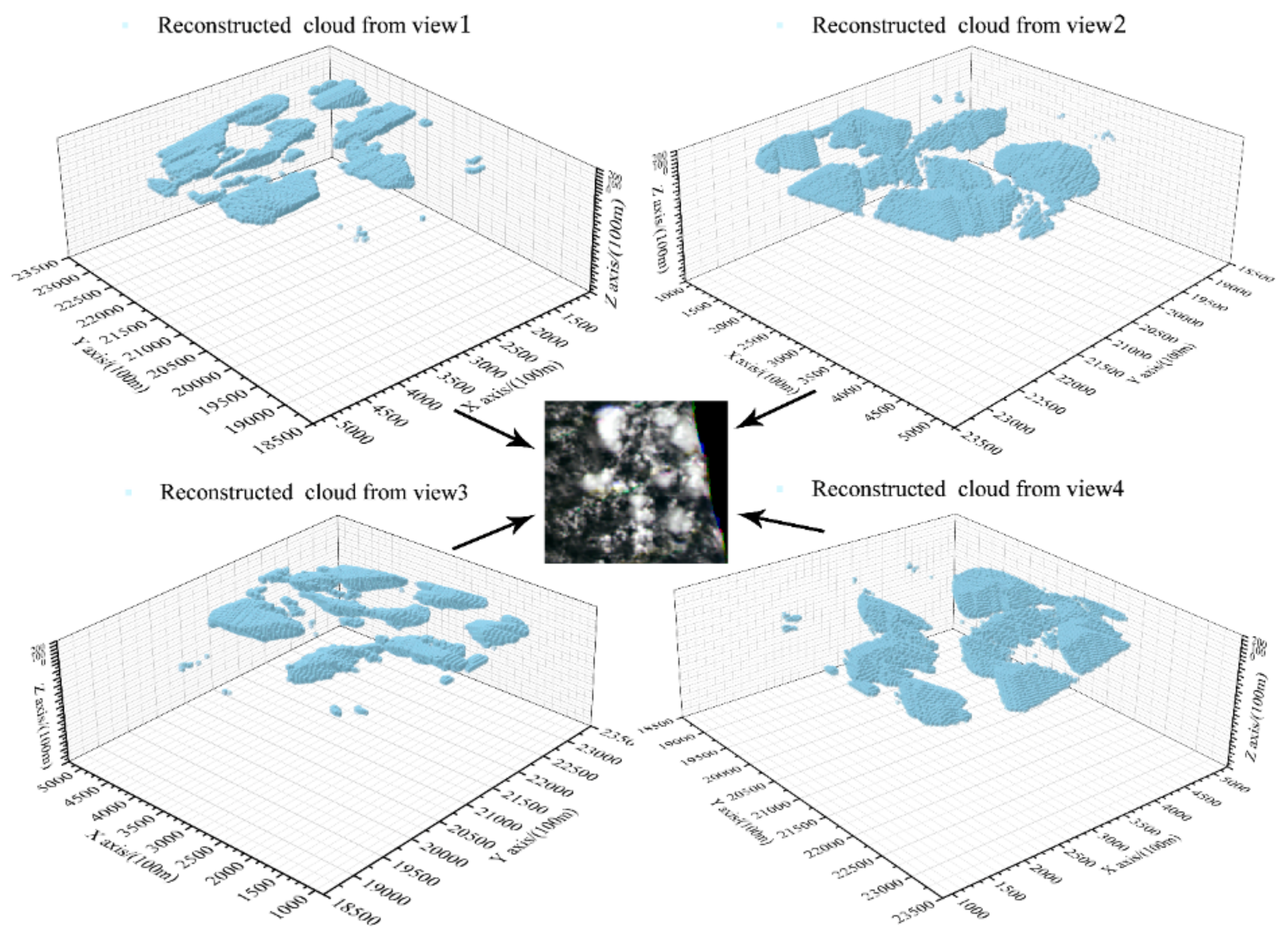
Figure 7.
The reconstruction results from four different viewing perspectives. The units are 100 m for a four-view direction. Red-Green-Blue (RGB) image shoots form the zenith direction of Directional Polarimetric Camera (DPC) at the center. The arrow corresponds to the different angle of observation.
Figure 8.
Binary cloud mask of all angles in the desert of the outback in Australia. Pink cloud mask is the result of cloud detection for each angle in the reconstructed region. White cloud mask is the result of cloud detection for each angle in the other region. The cloud detection is only for the area above the land in sample 1.
Figure 9.
Cloud casting path for each effective angle based on
Figure 8’s results. The different path in the same voxel model have the same vertical development. The ray casting path between different angles has regular changes in vertical development. In order to indicate the direction more clearly, a direction axis has been added, showing the north, east, and zenith direction.
Figure 10.
3-D cloud reconstructed results based on the distance threshold (DTH). The observed direction is the same with the view’s angle of
Figure 9 in the left image. (
a) rotates 90° counter-clockwise, which is seen in (
b).
Figure 10.
3-D cloud reconstructed results based on the distance threshold (DTH). The observed direction is the same with the view’s angle of
Figure 9 in the left image. (
a) rotates 90° counter-clockwise, which is seen in (
b).
Figure 11.
Description and comparison of the location of verification for sample 1. The blue line is a track of CALIOP satellite above the Red-Green-Blue (RGB) image of Moderate Resolution Imaging Spectroradiometer (MODIS) in (a). The red line is an extraction path of reconstruction above the RGB image of Directional Polarimetric Camera (DPC) in (b). The position of the red line is translated from the blue line, based on the relative position of the cloud. In (c), the red strip is the extraction of the 3-D cloud reconstruction result along an offset track of CALIOP. The latitude of comparison is from DPC data. The pink strip is an overestimated part in the center of the cloud and this overestimated situation is a good point for a future research work. The blue strip shows cloud of the Vertical Feature Mask (VFM) of Cloud-Aerosol Lidar with Orthogonal Polarization (CALIOP). For these different situations in the dotted box A~E, a detailed analysis is carried out in this paper.
Figure 12.
Similar to
Figure 8, the binary cloud mask of all angles in the Atlantic Ocean near Western Africa. The pink cloud mask is the result of cloud detection for each angle in a reconstructed region. The white cloud mask is the result of cloud detection for each angle in the other region. The cloud detection is only for the area above the land in sample 2.
Figure 13.
Similar to
Figure 9, but for sample 2. The ray casting path for each effective angle reconstruction based on
Figure 12’s results.
Figure 13.
Similar to
Figure 9, but for sample 2. The ray casting path for each effective angle reconstruction based on
Figure 12’s results.
Figure 14.
Same as in
Figure 10, 3-D cloud reconstructed results based on the distance threshold (DTH). The observed direction is the same with the view’s angle of
Figure 9 in (
a). (
a) rotates 90° counter-clockwise, which is in (
b).
Figure 14.
Same as in
Figure 10, 3-D cloud reconstructed results based on the distance threshold (DTH). The observed direction is the same with the view’s angle of
Figure 9 in (
a). (
a) rotates 90° counter-clockwise, which is in (
b).
Figure 15.
Same as in
Figure 11, the description and comparison of the location for sample2’s verification. The blue line is a track of CALIOP satellite above the Red-Green-Blue (RGB) image of Moderate Resolution Imaging Spectroradiometer (MODIS) in (
a). The red line is an extraction path of reconstruction above the RGB image of Directional Polarimetric Camera (DPC) in (
b). The comparison between product of CALIOP and section of reconstruction is shown in (
c). The latitude of comparison is from DPC data. Different situations are shown in the dotted box from A to C. a specific description is carried out in this paper.
Figure 16.
The 3-D extraction result from the clouds’ reconstruction. Size of clouds is small in sample 2,
Figure 15c 3-D representation. In this section, the dashed box corresponds to the dashed box of
Figure 15c. Voxel of 3-D cloud is shown in a light blue color and extraction voxels of the 3-D cloud is given in a pink color.
Table 1.
The corresponding relation between the range of α and the direction of x and y.
Table 1.
The corresponding relation between the range of α and the direction of x and y.
| The Rang of α | Direction of x | Direction of y |
|---|
| 0° < α < 90° | north | east |
| 90°<< 180° | south | east |
| 180°<< 270° | south | west |
| 270°<< 360° | north | west |
Table 2.
The result of cloud detection and coverage of each view for sample 1 (unit: pixel).
Table 2.
The result of cloud detection and coverage of each view for sample 1 (unit: pixel).
| Observation | Invalid Value | Cloud | Clear | Coverage of Cloud | Coverage of Valid Value |
|---|
| Total: 10,201 |
|---|
| view 1 | 8202 | 1844 | 155 | 92.25% | 19.60% |
| view 2 | 3690 | 4938 | 1573 | 75.84% | 63.83% |
| view 3 | 7 | 6189 | 4005 | 60.71% | 99.93% |
| view 4 | 0 | 5305 | 4896 | 52.00% | 100.00% |
| view 5 | 0 | 4548 | 5653 | 44.58% | 100.00% |
| view 6 | 0 | 3969 | 6232 | 38.91% | 100.00% |
| view 7 | 0 | 3735 | 6466 | 36.61% | 100.00% |
| view 8 | 0 | 3909 | 6292 | 38.32% | 100.00% |
| view 9 | 0 | 4292 | 5909 | 42.07% | 100.00% |
| view 10 | 0 | 5132 | 5069 | 50.31% | 100.00% |
| view 11 | 3677 | 3884 | 2640 | 59.53% | 63.95% |
| view 12 | 9053 | 789 | 359 | 68.73% | 11.25% |
Table 3.
The comparison of precision between the section of the 3-D cloud and CALIOP in sample 1.
Table 3.
The comparison of precision between the section of the 3-D cloud and CALIOP in sample 1.
| Precision (km) | PASS | Total Number | Correct |
|---|
| (0, 0.1] | 73 | 116 | 62.93% |
| (0.1, 0.2] | 74 | 116 | 63.79% |
| (0.2,0.3] | 77 | 116 | 66.38% |
| (0.3,0.4] | 77 | 116 | 66.38% |
| (0.4, 0.5] | 79 | 116 | 68.10% |
| (0.5, 0.6] | 81 | 116 | 69.83% |
| (0.6, 0.7] | 81 | 116 | 69.83% |
| (0.7, 0.8] | 81 | 116 | 69.83% |
| (0.8, 0.9] | 83 | 116 | 71.55% |
| (0.9, 1.0] | 86 | 116 | 74.14% |
Table 4.
The result of cloud detection and coverage of each view for sample 2 (unit: pixel).
Table 4.
The result of cloud detection and coverage of each view for sample 2 (unit: pixel).
| Observation | Invalid Value | Cloud | Clear | Coverage of Cloud | Coverage of Valid Value |
|---|
| Total: 15,416 |
|---|
| view 1 | 124 | 4204 | 11,088 | 27.49% | 99.20% |
| view 2 | 0 | 4147 | 11,269 | 26.90% | 100.00% |
| view 3 | 0 | 3875 | 11,541 | 25.14% | 100.00% |
| view 4 | 0 | 3895 | 11,521 | 25.27% | 100.00% |
| view 5 | 0 | 3825 | 11,591 | 24.81% | 100.00% |
| view 6 | 0 | 3905 | 11,511 | 25.33% | 100.00% |
| view 7 | 0 | 3900 | 11,516 | 25.30% | 100.00% |
| view 8 | 0 | 3517 | 11,899 | 22.81% | 100.00% |
| view 9 | 6415 | 1773 | 7228 | 19.70% | 58.39% |
| view 10 | 13,052 | 382 | 1982 | 16.16% | 15.33% |
| view 11 | 12,524 | 292 | 2600 | 10.10% | 18.76% |
| view 12 | 5821 | 2696 | 6899 | 28.10% | 62.24% |
Table 5.
The comparison of precision between a section of the 3-D cloud and CALIOP in sample 2.
Table 5.
The comparison of precision between a section of the 3-D cloud and CALIOP in sample 2.
| Precision (km) | PASS | Pass of Dashed C | Total Number | Number of Dashed C | Correct | Correction of Dashed C |
|---|
| (0, 0.1] | 9 | 4 | 30 | 11 | 30.00% | 36.36% |
| (0.1, 0.2] | 16 | 10 | 30 | 11 | 53.33% | 90.91% |
| (0.2,0.3] | 16 | 10 | 30 | 11 | 53.33% | 90.91% |
| (0.3,0.4] | 16 | 10 | 30 | 11 | 53.33% | 90.91% |
| (0.4, 0.5] | 16 | 10 | 30 | 11 | 53.33% | 90.91% |
| (0.5, 0.6] | 17 | 10 | 30 | 11 | 56.67% | 90.91% |
| (0.6, 0.7] | 19 | 10 | 30 | 11 | 63.33% | 90.91% |
| (0.7, 0.8] | 20 | 10 | 30 | 11 | 66.67% | 90.91% |
| (0.8, 0.9] | 20 | 10 | 30 | 11 | 66.67% | 90.91% |
| (0.9, 1.0] | 20 | 10 | 30 | 11 | 66.67% | 90.91% |
© 2019 by the authors. Licensee MDPI, Basel, Switzerland. This article is an open access article distributed under the terms and conditions of the Creative Commons Attribution (CC BY) license (http://creativecommons.org/licenses/by/4.0/).

 ,
, 


