1. Introduction
Satellite synthetic aperture radar (SAR) has been used for operational surveillance of large sea areas and the detection of marine oil spills for decades. Still, several challenges remain, including the separation between oil spills and other low backscatter phenomena, and the description of oil spill properties from SAR. Distinguishing between thicker actionable oil spills of large volumes and non-actionable thin slicks is one of the challenges for the SAR-based operational services.
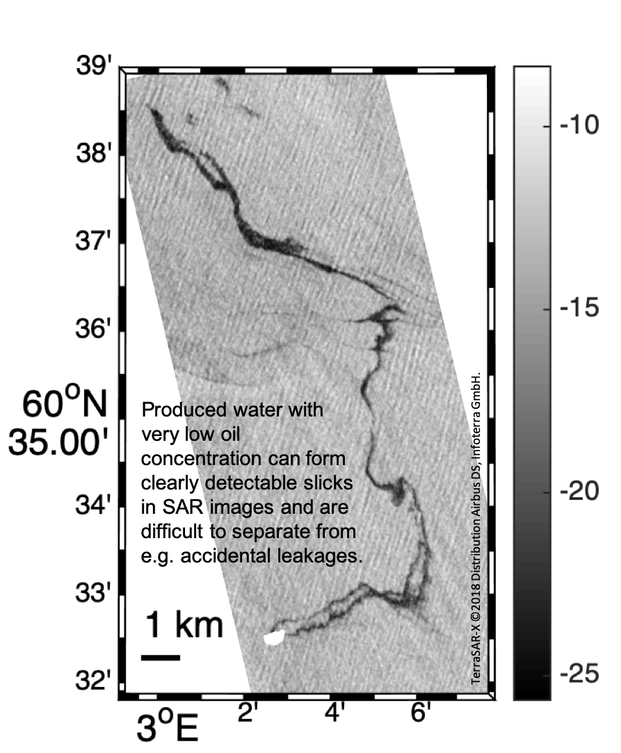
Oil slicks resulting from releases of produced water (PW) are frequently detected around oil platforms in the North Sea. The PW is water that is brought to the surface together with oil and gas from the reservoir, and after treatment still contains some oil. When PW is released into the sea, it produces a thin surface slick. Releases of PW are legal within certain limitations. From Norwegian platforms alone, more than 133 million m
of PW was released in 2018, with an average oil concentration of 11.2 g/m
[
1]. Separating these slicks from other types of oil spills is difficult, although the proximity to a platform can be used as an indication. However, distinguishing between normal discharges of PW and possible abnormal events with elevated releases or accidental leakage is difficult. Hence, PW poses a challenge for the operational oil spill detection services and may lead to missed detections of actual oil spills. Very little research has been done on these type of oil slicks and their characteristics in SAR images.
For this paper, high-resolution dual-polarization (HH/VV) TerraSAR-X data have been systematically collected over one platform, together with in situ information about PW release volumes and oil concentrations. The sensor properties and oil type are constant throughout the data set, allowing for comparison in terms of release volumes. The objective of this work is to investigate the characteristics of SAR signatures of PW, including their typical appearance in HH/VV SAR data, possible variations with oil release volume, and limitations on detectability in terms of oil releases and wind conditions.
The study shows that even very small oil concentrations (volume percentage of 0.001%–0.002% in this data set) produce clearly detectable SAR signatures, with damping ratios around 3–9 dB, which is comparable to observations over high concentration oil releases. Hourly average oil release volumes as small as 0.003 m (accumulated daily volume before SAR overpass as low as 0.04 m) are detected. Slicks are detected in wind speeds of 2–12 m/s, with reduced detectability at least above 9 m/s. A clear correlation with release volume is not found for the investigated parameters, but some trends that are observed should be further investigated when data with larger releases are available.
The paper is organized as follows.
Section 2 contains some background information and describes the investigated parameters.
Section 3 presents the data set, and
Section 4 contains the results.
Section 5 concludes the paper.
2. Background
Operational PW releases from platforms contain mineral oil, but the oil concentration is very low and it does not form actionable oil slicks. However, areas where PW frequently occurs may cause misinterpretation if there is a larger spill, accidental leakage, etc., which may be falsely classified as PW. Even though monitoring of the oil production sites is a daily task for satellite service providers, to the authors’ knowledge, the remote sensing of PW slicks specifically, has not previously been addressed in the literature.
Traditionally, single-polarization parameters related to geometry, shape, contrast, gradients, and contextual information have been used for oil spill detection and oil vs. look-alike discrimination [
2]. These parameters are still used today in operational oil spill services, which are based on single-polarization low-resolution SAR scenes with large spatial coverage. Over the past decade or so, a lot of the research within oil spill remote sensing has focused on the possible use of polarimetry to enhance the detection and characterization of slicks (see, e.g., [
3,
4,
5,
6,
7,
8,
9,
10,
11] and references therein). Some studies have indicated a possibility for improved oil spill vs. look-alike discrimination and description of slick properties. Still, no polarimetry-based methods have been thoroughly tested for large data sets and found to show consistently good and reliable results, hence being ready for operational use. In addition, sensor noise and its effect on polarimetric measurements and interpretation is a challenge, particularly for spaceborne sensors (see, e.g., [
12,
13]).
In this work, produced water oil slicks are investigated using a few simple parameters that are based on one or two co-polarization channels (vertical transmit and receive (VV) and/or horizontal transmit and receive (HH)). The single-polarization damping ratio (DR) is often used as an oil-sea contrast measure. Several studies also suggest a relation between DR and oil slick thickness variations [
14,
15,
16,
17,
18]. However, the data material is limited, and the actual relation, validity conditions, and limitations are not mapped out. The DR of the VV channel is here investigated as this channel generally produces a better contrast than HH [
5]. The DR is defined as
where
and
denote the mean intensity of the measured complex scattering coefficient
S for vertical transmit and receive polarization within clean sea and oil slick pixels, respectively. To reduce speckle, the image is first multilooked using a
pixel window. Different window sizes were tested and 21 was found to give good speckle reduction while keeping sufficient detail. The DR is subsequently calculated for each pixel using the clean sea mean value at the exact same range position (exact same incidence angle). The clean sea mean is an average of over 800 azimuth pixels at each range position.
In addition to DR, two common dual-polarization parameters are investigated, i.e., the polarization difference (PD) and the co-polarization power ratio (CPR). These are defined as
and
In the scattering model described in [
19], the SAR ocean backscatter is expressed as the sum of two components, i.e., one polarization-dependent part related to the two-scale Bragg scatter model and one nonpolarized part. In PD, the nonpolarized component is removed, and this parameter is, therefore, controlled by the small-scale wave components close to the Bragg wavenumber and should reveal near-surface wind variability and presence of slicks [
19]. The PD has been found to give a very good oil-sea contrast for C- and L-band data in, e.g., [
8,
19,
20,
21,
22], and to be less sensitive to incidence angle and proximity to noise floor than other multipolarization features [
13,
21].
The CPR has been applied in many oil spill studies, see e.g., [
5,
6,
8,
19,
21]. A particularly interesting property of this feature is its independence of small-scale roughness within the tilted Bragg model, indicating that a change in the effective dielectric constant is necessary in order for this parameter to detect an oil slick, i.e., a thick slick or high concentration of oil in the surface water is needed [
5,
8]. The CPR was used to estimate the oil content in oil-water mixtures in [
5,
11]. An increase (decrease) in the value of CPR (PD) is expected when moving from a slick-free to an oil-covered surface (see, e.g., [
5,
21]). Normalized versions of PD and CPR (PDc and CPRc) are also extracted, where the clean sea mean in each parameter is divided by the corresponding slick values, similar to the calculation of DR.
Using these parameters, SAR detections of PW are analyzed here to investigate the typical values and behavior of this type of surface film. Parameters are compared to in situ measurements in order to investigate the effect of increasing oil volume on the SAR signature, and in particular on the oil-sea contrast in DR and PD and to explore if there are any parts of the slick that affect the CPR. As thicker oil may produce more internal zoning and thickness variations, the degree of internal variation is also of interest. The results of this analysis are presented in
Section 4.
3. Data Set
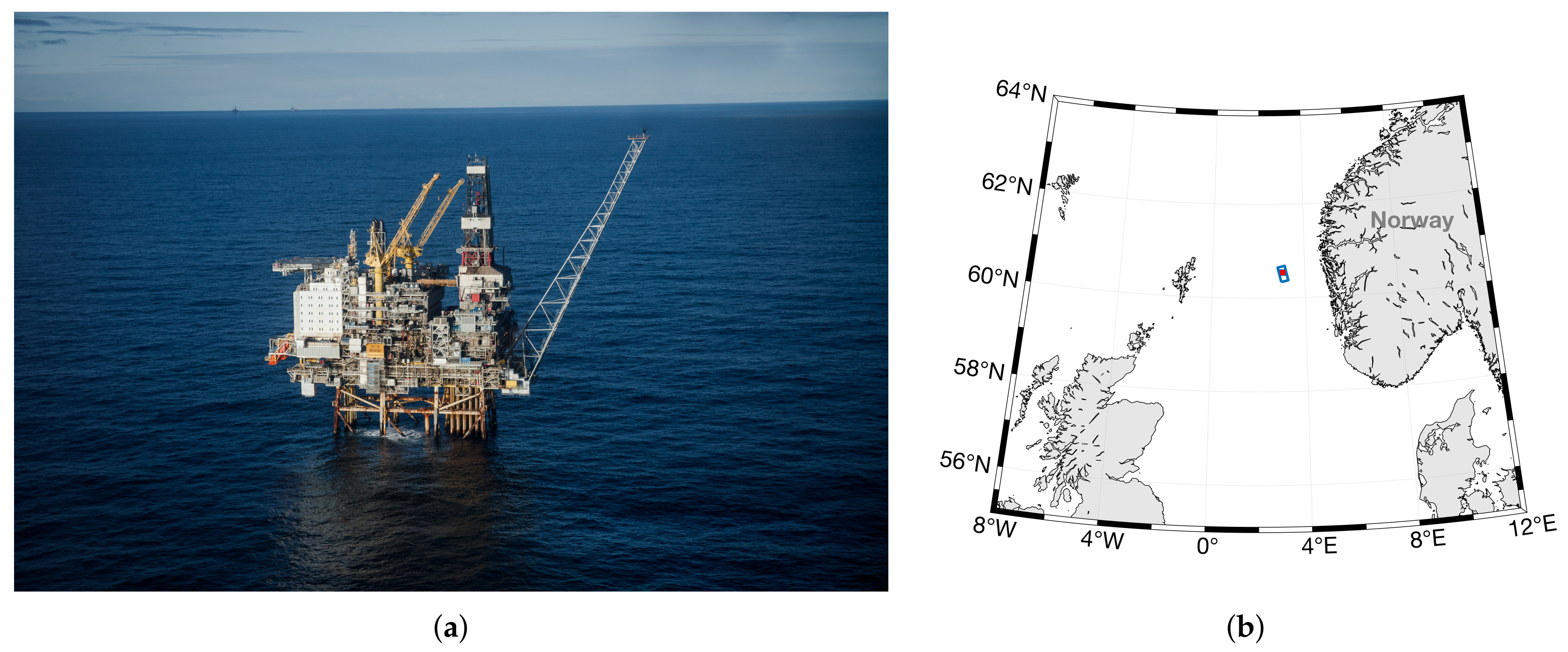
For this study, the platform Brage, located in the North Sea, about 120 km northwest of Bergen (60.5425
N, 3.0468
E) was selected as a test site, as it is one of the platforms where PW is frequently detected. A photograph of the Brage platform and the location of both the platform and the satellite data are shown in
Figure 1. For the past few years, multipolarization SAR data have been systematically collected over Brage during the summer months when the wind conditions are relatively calm and favorable for SAR based oil detection. At the same time, in situ measurements have been acquired at the platform. The data are described in the following sections.
3.1. SAR Data
To limit the number of SAR related variables, this study is based only on TerraSAR-X data acquired in the stripmap dual-polarization (HH/VV) mode. This mode provides scenes with a coverage of 15 × 50 km (range × azimuth), an azimuth resolution of 6.6 m and a ground range resolution between 1.7 m and 3.49 m, depending on the incidence angle [
23]. All scenes are acquired in beam stripNear005, i.e., the oil slick is located at incidence angles between 25.5
–26
in each scene. In total, 10 scenes from the summers of 2018 and 2019 are included in this analysis. Having the exact same SAR configuration and oil type in all scenes makes it easier to conduct a comparison in terms of release properties such as volume and oil concentration. The wind and wave conditions can vary among the scenes, but this study is mainly limited to low-medium wind conditions <5–6 m/s.
Table 1 and
Table 2 give an overview of the SAR scenes and corresponding in situ information.
3.2. In Situ Data
The data collection was done in cooperation with Wintershall which is the operator of the Brage platform. In addition to the release information that is routinely logged at the platform, sample measurements were acquired ca 10 min and 130 min before the satellite overpasses. The in situ information used here include the oil concentration in the two samples as well as a daily mean concentration, and hourly release volumes of produced water. The concentration measures and selected volumes are presented in
Table 1.
As can be seen from
Table 1, the three concentration values per day show relatively small variations within one day and also among the ten scenes. The values lie between 7.5–18 g/m
for the 130 min sample and 7–13.8 g/m
for the daily means.
Produced water at Brage is released continuously from 17 m below the sea surface, from which the PW rises to the surface and forms a slick. The slick is influenced by wind, waves, and currents, and its properties are altered through different weathering processes [
24]. The SAR detected slick area consists of the PW released over an unknown period of time, and it is difficult to know exactly when the different parts of the slick were discharged. In this study, the releases from two different time periods are evaluated for each SAR scene, i.e., (i) the release done before the SAR overpass on the day of acquisition (00:00–17:00) and (ii) the release done over the last four hours prior to overpass (13:00–17:00). The latter time period is selected as an in situ sample was taken about 130 min before the satellite overpasses. It is assumed that this concentration measure is representative of the release done during the four hour time period. In
Table 1, the total release volume for approximately four hours and 17 h before overpass is provided for each scene. The volumes vary between ca 1000–4000 m
and 4000–17,000 m
, respectively. The volume of the oil component in the PW is also included in
Table 1. This is estimated using the 130 min sample concentration for the four hour case and the daily mean concentration for the 17 h case. This results in oil volumes of 10–49 kg (or 0.01–0.06 m
using a density of 826 mg/m
[
25]), and 36–234 kg (0.04–0.28 m
), respectively. The volume percentage of the oil component is then only 0.001%–0.002%. The daily mean release per hour lies between 230–1060 m
for PW and 0.003–0.018 m
for the oil component. These are typical numbers for the Brage platform, which in 2018 had an estimated average of 227 kg of oil released per day (i.e., ca 161 kg for 17 h) and an average PW oil concentration of ∼ 16 g/m
. For comparison, the limit for legal releases according to the Convention for the Protection of the Marine Environment of the North-East Atlantic (OSPAR) are monthly average concentrations of 30 g/m
[
26].
To select the slick region assumed to represent the last four hours of release, the expected drift length over four hours is estimated using the rule-of-thumb of an approximate drift speed of 3% of the wind speed [
27]. Information on wind conditions is logged at Brage every 10 min, and
Table 2 presents wind measurements for each of the SAR scenes, including the measurement closest in time to SAR overpass (i.e., two minutes before), as well as the mean wind over the preceding four and 17 h. The mean wind speed in the four hour period is used to estimate the approximate drift in this time period, and all slick pixels within this distance is included in a new subslick region of interest (ROI). For some scenes, the entire slick is within this distance and included in the analysis. In other cases, only a small part of the SAR detection is included, as the slick extent is much larger than the expected four hour drift. The results presented in
Section 4 considers both the full slick, which is compared with the 17 h release information, and the subslick defined from the drift estimate, which is compared to the four hour release information.
It can be seen from
Table 2 that the data set is acquired mainly under low-medium wind conditions, with four (17) hour mean values between 1.6–5.4 m/s (3.2–6.4 m/s) for all scenes except #4 and #10 which has values around 9–10 m/s. The wind at the time of SAR acquisition, however, is still relatively low for scene #4 (5.4 m/s).
In addition to the scenes described in
Table 1 and
Table 2, five scenes were collected where PW slicks could not be clearly identified. In two of these, the area around Brage was dominated by large dark regions, likely due to low wind regions reducing the surface roughness. The wind speed at Brage at these times were 1.3 m/s and 1.8 m/s. Hence, any PW slicks present could not be separated from the clean, calm sea surface. For one of the scenes, the closest wind speed measures were around 9 m/s, and the surface may be too rough to detect slicks or to enable the PW to form slicks at all. The two remaining scenes were acquired on days with production halt and hence very little or no release.
3.3. SAR Data Quality
For low backscatter regions such as oil spills, the sensor’s background noise can be a challenge, resulting in a poor signal-to-noise ratio (SNR). This may affect the backscatter values and multi-polarization parameters, possibly reducing the characterization ability and cause misinterpretations [
5,
12,
13,
21].
To assess the SAR data quality, the signal-to-noise ratio (SNR) is calculated for each pixel by comparing the pixels backscatter value, , with the noise equivalent sigma zero (NESZ) at the same incidence angle (both in linear units), using
Note that the NESZ is subtracted before taking the ratio, i.e., the actual signal above NESZ, not the measured signal is used (see [
13]).
Figure 2 shows the range of SNR values within the slick regions. The vertical lines are plotted between the 5th and 95th percentiles (small dots), and the 50th percentiles are indicated by a star (diamond) for VV (HH). Colors changes from light to dark blue with increasing release volume. Clean sea (CS) values are included in gray.
In [
13], a limit of SNR = 10 dB is suggested in order for the data to be useful for polarimetric scattering analysis.
Figure 2 shows that the median SNR values for the clean sea lie between 11–18 dB, and all scenes but one have their 5th percentile above 10 dB. For the slicks, the SNR median lies between ca 0–13 dB (mostly above 6 dB) for VV and −2 to 13 dB (mostly above 6 dB) for HH. Hence, part of the data lie below the recommended limit. A detailed scattering analysis is not the objective of this study, and a lower SNR can be accepted. However, the proximity to the noise floor and possible effects on the results should always be kept in mind when analyzing this type of data.
In addition to the sensor background noise, other noise sources may also affect the measurements. The slicks are close to the platform which is a strong point target, possibly altering the backscatter values. The sea surface closest to the platform is not included in the segmented ROI, but the selected area could be somewhat affected by the platform target. Different noise sources are described and investigated for the oil spill case in [
13].
4. Results
The parameters defined in
Section 2 are extracted for each of the scenes described in
Section 3.
Figure 3,
Figure 4,
Figure 5 and
Figure 6 shows the intensity images and evaluated parameters for four of the scenes. Note that the geographical area and the color bar are not equal for the different scenes.
Figure 3,
Figure 4,
Figure 5 and
Figure 6 show that the PW slicks are easily identified in the intensity images and that the size and shape vary a lot among the scenes. Across the 10 scenes, the approximate area of the segmented slicks lies between 0.2 and 5.2 km
, and the distance from the platform to the furthest point (along the line of sight) varies between 1.5 and 11.7 km. The DR (
Figure 3b,
Figure 4b,
Figure 5b and
Figure 6b) clearly shows the PW with values up to 10–12 dB in these cases and some internal variation in the contrast is observed. The PD (
Figure 3c,
Figure 4c,
Figure 5c and
Figure 6c) has relatively low oil-sea contrasts and it is more difficult to visually identify the boundary between slicks and clean sea in this parameter. In the CPR images (
Figure 3d,
Figure 4d,
Figure 5d and
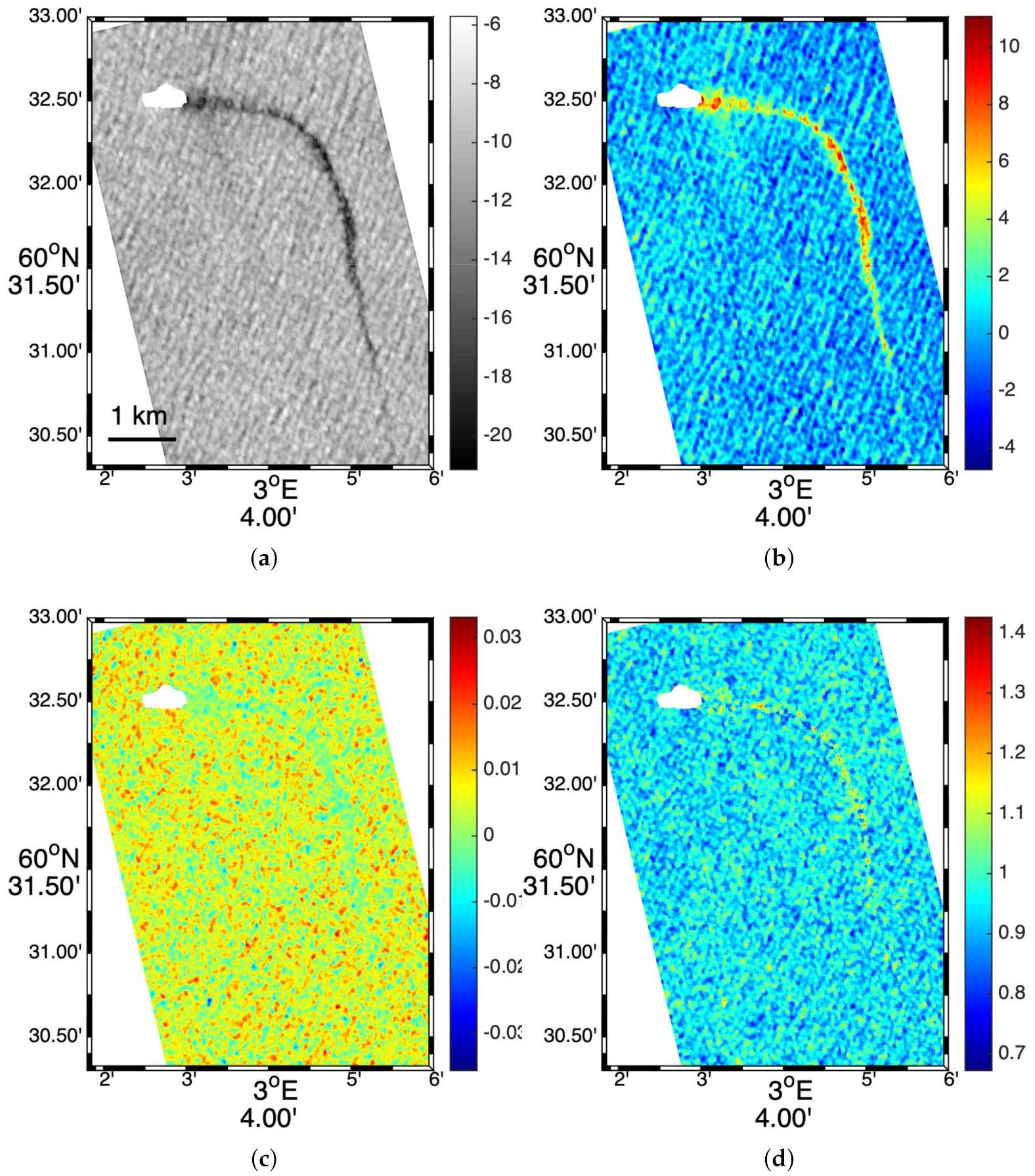
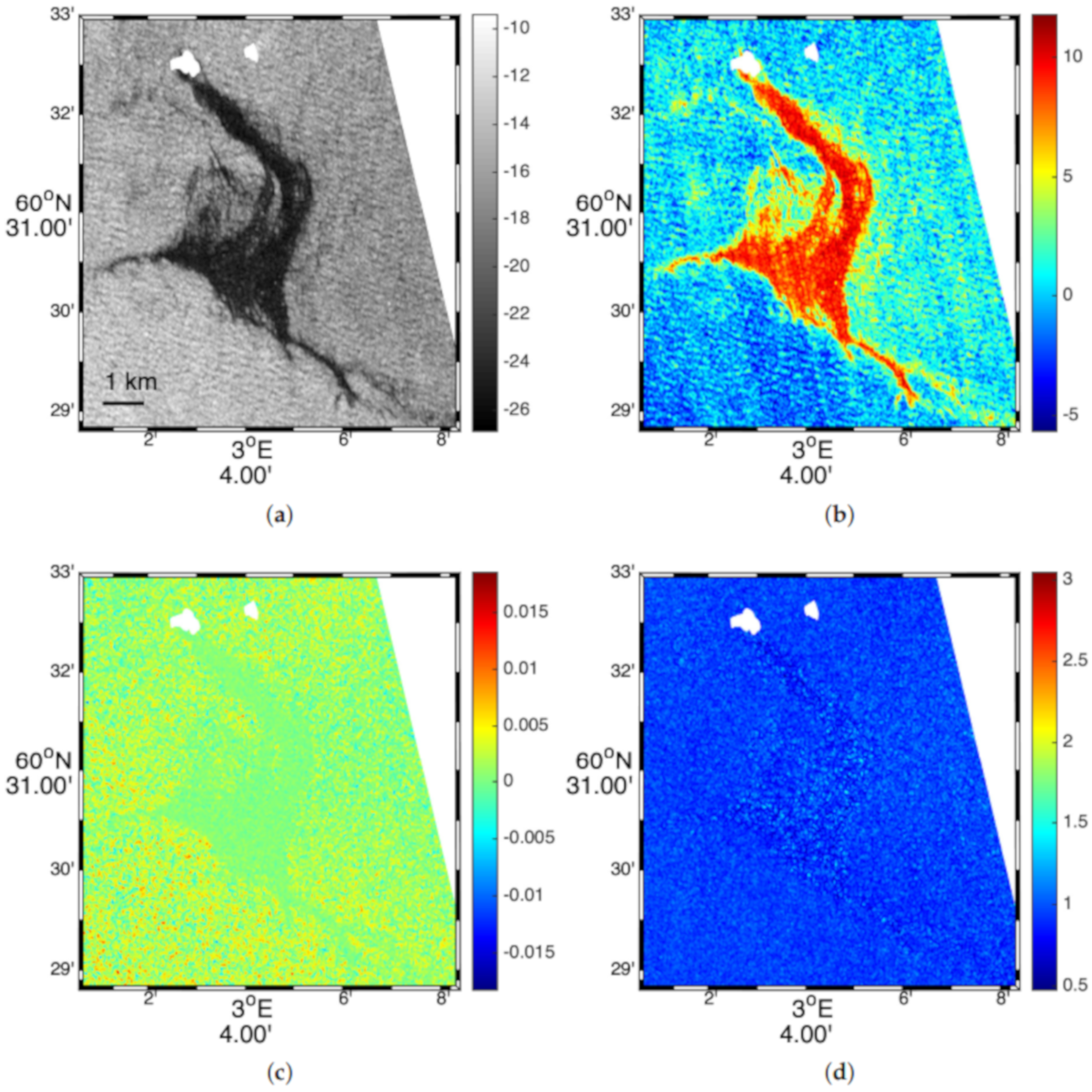
Figure 6d), only parts of the slicks are seen as discontinuous areas of increased values. These may be areas where the dielectric constant is affected by the presence of oil, due to thicker oil layers or higher concentration of oil in the water column. For the rest of the slick, the oil layer may not be thick enough to affect the dielectric constant of the surface, and in turn the CPR. As the oil concentrations at the time of release are very low, a change in the surface dielectric properties is not expected. However, the oil in the PW may concentrate at the surface, possibly forming thicker layers that may have some effect on the dielectric constant (see further discussion below).
Comparing scenes and parameters visually is difficult, and a more detailed investigation of the actual parameter values and their connection to release properties are presented in the next sections.
4.1. Parameter Values vs. Release Volumes—Full Slick
Figure 7 shows the range of feature values within the segmented oil slicks, from the 5th to the 95th percentiles. The 50th percentile is indicated with a star. In the left column, the ranges of clean sea values are included in gray, with a circle indicating the median. These values are based on the CS region selected at the same range position as the slick and used to produce the DR, PDc, and CPRc. The full slick region is compared to the releases done over the 17 h prior to the satellite acquisition (see
Section 3.2).
From
Figure 7a, we see that the backscatter values vary among scenes for both slicks and clean sea. The medians lie around –24 dB to –14 dB for slicks and –16 dB to –10 dB for clean sea. The slick-sea contrast is quantified by the DR shown in
Figure 7b with median values from 3–9 dB. HH (not shown) produces very similar results as VV but with overall slightly lower intensity and DR values. These DR values are similar to previously observed values for mineral oil slicks in the same data mode [
20,
21].
For PD in
Figure 7c, the PW slicks and clean sea have very similar values, with the clean sea median generally slightly above the slick median. PD is expected to be positive as VV generally has higher backscatter than HH over ocean regions. However, in this data set, all scenes have both positive and negative values in both clean sea and slick-covered areas. For a few scenes, even the median is negative (scene #8 and #10 for oil slicks, scene #9 and #10 for clean sea). Although PD has been found to produce high slick-sea contrasts in many previous studies using C- and L-band SAR, this is not the case here. Lower PD contrasts have also been observed in TerraSAR-X data previously [
20], and could be due to data quality.
The CPR in
Figure 7e shows median values generally between 0.9 and 1 for both clean sea and slicks. The two regions have overlapping values and similar medians, and hence the CPRc lies close to 1. Previous work has shown higher CPR values for slick-covered areas than for clean sea. The results in
Figure 7e,f shows the opposite for most scenes, although the differences are small. Similar CPR values in PW and clean sea may indicate that the slicks are too thin to significantly affect the dielectric properties of the surface. Assuming the total volume released in the investigated time period is forming a homogeneous surface film that is fully detected by SAR, the film thicknesses (estimated from the SAR area and approximate volumes given in
Table 1) lie in the range 0.02–1.3
m. This belongs to the sheen and rainbow classes under the Bonn Agreement Oil Appearance Code [
28] and is considered not actionable oil. However, the slick thickness of mineral oil spills is heterogeneous, and some parts may be thicker, possibly causing smaller areas of increased CPR as can be seen in
Figure 3,
Figure 4,
Figure 5 and
Figure 6.
Also CPR shows that
in parts of the data. This could be partly related to the relatively low incidence angles, as the difference between the channels increases at larger angles. In the oil slick regions, a higher signal damping in VV than in HH may result in PD < 0 and CPR > 1. In [
13] it is shown that for noise only, PD and CPR would take values of 0 and 1, respectively. Hence, the results in
Figure 7 may indicate that the noise may have a large effect on our data set and that the SNR is too low for a detailed comparison like this. The somewhat unexpected values of PD and CPR and possible noise effects should be further investigated in future work.
There is no clear, consistent correlation between the parameters and oil release volume. This may not be surprising, considering the relatively low variation in the release concentrations and volumes among scenes. However, some indications of potential trends can be observed. DR seems to increase for higher release volumes for the low-medium wind scenes (i.e., excluding scene #10). Also, the three scenes with the highest releases (scenes #1, #5, and #7) have lower median CPR values and larger internal variations compared to the other scenes in PDc, and to some degree in CPR and CPRc. These observations should be further investigated when a larger data set, with more variability in oil volume and also larger releases, is available.
As seen in
Table 2, scene #10 is the only scene with consistently high wind conditions in the period before and during SAR acquisition. It can be noticed that this scene has the highest backscatter value, lowest DR and also overall less internal variation in parameter values compared to the low-medium wind scenes.
4.2. Parameter Values vs. Release Volumes—Subslick
Figure 8 shows the same results as presented in
Figure 7, only for the part of the slick within the four hour drift estimate (see description in
Section 3.2) and the estimated release volume in this period (see
Table 1).
Overall, the results are similar to those for the full slick in
Figure 7. For all scenes, the full slick and subslick DR values are similar, or slightly higher (up to 1.4 dB) in the full slick case. Hence, the damping in the part of the slick most recently released is not higher than in the total slick. The same is observed in PDc and CPRc, with slightly higher contrasts in the full slick for the majority of the scenes.
None of the parameters show a clear correlation with oil volume. The indications of possible trends with oil volume observed in the full slick case is not seen in the subslick case.
5. Conclusions
Produced water is detected frequently close to oil production platforms and it is a challenge for operational services to distinguish normal operational releases from abnormal events or accidental leakages. In this work, a unique data set of high-resolution dual-polarization (HH/VV) TerraSAR-X data with constant observation geometry is collected over produced water from one selected platform to investigate typical behavior of these slicks in SAR images.
It is seen that even very small amounts of oil produce clearly detectable slicks. The slicks in this data set cover areas up to more than 5 km and extend up to almost 12 km from the platform. Although the subsurface releases have oil concentrations as low as 7–19 g/m (volume percentage of 0.001%–0.002%), the oil seems to concentrate on the surface, forming a slick with probably much higher oil-to-water ratio. The total oil volumes are still small, with the volume of the oil component released prior to SAR acquisition on the observation day estimated to 0.04–0.28 m. These are typical PW releases and well within the legal limit. Even these small volumes produce easily detectable slicks, with median damping ratios of 3–9 dB in both HH and VV. When comparing the signature of the full slick and the part of the slick most recently released, slightly higher oil-sea contrasts are found in the full slick case.
The VV damping ratio, as well as the dual-copolarization parameters PD and CPR and their contrasts, are investigated and show no clear correlation with release volume. This is not surprising considering the relatively low oil volumes and small variations among scenes. For the full slick, there is some indication of increasing DR for higher oil volume in the low-medium wind scenes, and of lower CPR and larger internal variation, especially in PDc, but this needs to be further investigated in the future. In the case of a crude oil release, or much larger PW concentration/volumes, a difference in parameter values, contrasts or internal variation may appear. Hence, it would be very interesting from both a research and an operational viewpoint to compare the collected data set with acquisitions containing large releases of the same oil type. However, this is difficult to plan for, and future work will look at this question also using scanSAR data, which will hopefully increase the spread in release volumes and increase the likelihood of imaging a high release event should it occur.
CPR only detects parts of the slick, which may be regions of thicker film or higher oil concentrations. Although PD is often found to produce very high oil-sea contrasts in C- and L-band data, we here find relatively low contrasts. This has also previously been observed for TerraSAR-X data and could be related to, e.g., data quality and/or system noise. The HH and VV backscatter values are very similar in these scenes, which may be partly due to the relatively low incidence angles of , also causing negative PD values and CPR > 1. However, the somewhat unexpected characteristics of PD and CPR in these scenes should be further investigated.
This data set, where the SAR configuration is kept constant, allows for some investigation of limitations on oil slick detectability, e.g., when it comes to oil volumes and wind conditions, which is also of interest for operational services. We here detect release volumes as low as 0.04 m if looking at the estimated oil release on the day of SAR acquisition prior to overpass. It is observed that these low concentration/small volume releases can be detected in wind conditions from 2–12 m/s, but detectability seems to decrease at least above ∼9 m/s. The one high wind scene produced the lowest damping ratio, and also a lower degree of internal variation in the parameter values, and clearly shows that different wind speed regimes must be considered when developing operational methods for distinguishing different release types.
This study confirms that even the very small oil volumes present in PW releases produce quite large damping ratios, comparable to values observed for much larger volumes and concentrations in other data sets, hence constituting a risk of falsely interpreting actual oil discharges or leakages as produced water. Future work will compare SAR parameters for a larger range of release volumes, and should also consider a larger set of parameters, possibly also including traditional features, e.g., related to size and shape. As all platforms are potential hot spots for produced water releases, a statistical database on typical SAR signatures from the specific site could be build-up and used as a reference to identify potential deviations from the normal. A similar mapping as here presented could also be carried out at other sensor frequencies, incidence angles, degree of multi-looking, etc., as well as for other oil types and platforms, other wind conditions, and the potential of combining these data sets should be evaluated.
Author Contributions
Conceptualization, S.S., A.M.J., and C.B.; formal analysis, S.S.; data curation, S.S. and A.M.J.; writing—original draft preparation, S.S. and A.M.J.; writing—review and editing, S.S., A.M.J., and C.B.; visualization, S.S.
Funding
This research was funded by the Norwegian Research Council projects; “Center for Integrated Remote Sensing and Forecasting for Arctic Operations” (CIRFA) (NFR project number 237906) and “Oil spill and newly formed sea ice detection, characterization, and mapping in the Barents Sea using remote sensing by SAR” (OIBSAR) (NFR project number 280616). The publication charges for this article have been funded by a grant from the publication fund of UiT The Arctic University of Norway.
Acknowledgments
TerraSAR-X images were provided by the German Aerospace Center (DLR) through TerraSAR-X AO MTH3174. In situ data were collected by Wintershall, and the authors wish to extend their thanks to all who participated in the data collection on-board the Brage platform. Meteorological data were provided by the Norwegian Meteorological Institute, though the web portal; eklima.met.no. The segmentation algorithm was developed by Martine M. Espeseth at UiT The Arctic University of Norway.
Conflicts of Interest
The authors declare no conflict of interest.
Abbreviations
The following abbreviations are used in this manuscript:
| SAR | Synthetic aperture radar |
| PW | Produced water |
| DR | Damping ratio |
| PD | Polarization difference |
| CPR | Co-polarization power ratio |
| PDc | Normalised polarization difference |
| CPRc | Normalized co-polarization power ratio |
| SNR | Signal-to-noise ratio |
| NESZ | Noise equivalent sigma zero |
| ROI | Region of interest |
References
- Norsk olje & Gass. Miljørapport, Olje- og Gassindustriens Miljøarbeid, Fakta og Utviklingstrekk; Technical report; Norsk olje & Gass: Sandnes, Norway, 2019. [Google Scholar]
- Brekke, C.; Solberg, A.H.S. Oil spill detection by satellite remote sensing. Remote Sens. Environ. 2005, 95, 1–13. [Google Scholar] [CrossRef]
- Lombardo, P.; Conte, D.I.; Morelli, A. Comparison of optimised processors for the detection and segmentation of oil slicks with polarimetric SAR images. IEEE Int. Geosci. Remote Sens. Symp. 2000, 7, 2963–2965. [Google Scholar] [CrossRef]
- Solberg, A.H.S. Remote sensing of ocean oil-spill pollution. Proc. IEEE 2012, 100, 2931–2945. [Google Scholar] [CrossRef]
- Minchew, B.; Jones, C.E.; Holt, B. Polarimetric analysis of backscatter from the Deepwater Horizon oil spill using L-band synthetic aperture radar. IEEE Trans. Geosci. Remote Sens. 2012, 50, 3812–3830. [Google Scholar] [CrossRef]
- Skrunes, S.; Brekke, C.; Eltoft, T. Characterization of Marine Surface Slicks by Radarsat-2 Multipolarization Features. IEEE Trans. Geosci. Remote Sens. 2014, 52, 5302–5319. [Google Scholar] [CrossRef] [Green Version]
- Migliaccio, M.; Nunziata, F.; Buono, A. SAR Polarimetry for sea oil slick observation. Int. J. Remote Sens. 2015, 32, 3243–3273. [Google Scholar] [CrossRef] [Green Version]
- Espeseth, M.M.; Skrunes, S.; Jones, C.E.; Brekke, C.; Holt, B.; Doulgeris, A.P. Analysis of Evolving Oil Spills in Full-Polarimetric and Hybrid-Polarity SAR. IEEE Trans. Geosci. Remote Sens. 2017, 55, 4190–4210. [Google Scholar] [CrossRef] [Green Version]
- De Maio, A.; Orlando, D.; Pallotta, L.; Clemente, C. A Multifamily GLRT for oil spill detection. IEEE Trans. Geosci. Remote Sens. 2017, 55, 63–79. [Google Scholar] [CrossRef]
- Pallotta, L.; Clemente, C.; De Maio, A.; Soraghan, J.J. Detecting covariance symmetries in polarimetric SAR images. IEEE Trans. Geosci. Remote Sens. 2017, 55, 80–95. [Google Scholar] [CrossRef]
- Angelliaume, S.; Boisot, O.; Guerin, C.A. Dual-Polarized L-Band SAR Imagery for Temporal Monitoring of Marine Oil Slick Concentration. Remote Sens. 2018, 10, 1012. [Google Scholar] [CrossRef] [Green Version]
- Alpers, W.; Holt, B.; Zeng, K. Oil spill detection by imaging radars: Challenges and pitfalls. Remote Sens. Environ. 2017, 201, 133–147. [Google Scholar] [CrossRef]
- Espeseth, M.; Brekke, C.; Jones, C.E.; Holt, B.; Freeman, A. The impact of system noise in polarimetric SAR imagery on oil spill observations. IEEE Trans. Geosci. Remote Sens. 2019. in print. [Google Scholar]
- Wismann, V.; Gade, M.; Alpers, W.; Hühnerfuss, H. Radar signatures of marine mineral oil spills measured by an airborne multi-frequency radar. Int. J. Remote Sens. 1998, 19, 3607–3623. [Google Scholar] [CrossRef]
- Gade, M.; Alpers, W.; Hühnerfuss, H.; Masuko, H.; Kobayashi, T. Imaging of biogenic and anthropogenic ocean surface films by the multifrequency/multipolarization SIR-C/X-SAR. J. Geophys. Res. Ocean. 1998, 103, 18851–18866. [Google Scholar] [CrossRef]
- Pinel, N.; Bourlier, C.; Sergievskaya, I. Two-Dimensional Radar Backscattering Modeling of Oil Slicks at Sea Based on the Model of Local Balance: Validation of Two Asymptotic Techniques for Thick Films. IEEE Trans. Geosci. Remote Sens. 2014, 52, 2326–2338. [Google Scholar] [CrossRef]
- Skrunes, S.; Brekke, C.; Espeseth, M.M. Assessment of the RISAT-1 FRS-2 Mode for Oil Spill Observation. IEEE Int. Geosci. Remote Sens. Symp. 2017. [Google Scholar] [CrossRef] [Green Version]
- Sergievskaya, I.; Ermakov, S.; Lazareva, T.; Guo, J. Damping of surface waves due to crude oil/oil emulsion films on water. Mar. Pollut. Bull. 2019, 146, 206–214. [Google Scholar] [CrossRef]
- Kudryavtsev, V.; Chapron, B.; Myasoedov, A.; Collard, F.; Johannessen, J. On Dual Co-Polarized SAR Measurements of the Ocean Surface. IEEE Geosci. Remote Sens. Lett. 2013, 10, 761–765. [Google Scholar] [CrossRef]
- Skrunes, S.; Brekke, C.; Eltoft, T.; Kudryavtsev, V. Comparing Near Coincident C- and X-band SAR Acquisitions of Marine Oil Spills. IEEE Trans. Geosci. Remote Sens. 2015, 53, 1958–1975. [Google Scholar] [CrossRef]
- Skrunes, S.; Brekke, C.; Jones, C.E.; Espeseth, M.M.; Holt, B. Effect of wind direction and incidence angle on polarimetric SAR observations of slicked and unslicked sea surfaces. Remote Sens. Environ. 2018, 213, 73–91. [Google Scholar] [CrossRef]
- Angelliaume, S.; Dubois-Fernandez, P.C.; Jones, C.E.; Holt, B.; Minchew, B.; Amri, E.; Miegebielle, V. SAR Imagery for Detecting Sea Surface Slicks:Performance Assessment of Polarization-Dependent Parameters. IEEE Trans. Geosci. Remote Sens. 2018, 56, 4237–4257. [Google Scholar] [CrossRef] [Green Version]
- German Aerospace Center. TerraSAR-X Ground Segment Basic Product Specification Document. 2013. Available online: https://sss.terrasar-x.dlr.de/docs/TX-GS-DD-3302.pdf (accessed on 2 December 2019).
- Reed, M.; Johansen, Ø.; Brandvik, P.J.; Daling, P.; Lewis, A.; Fiocco, R.; Mackay, D.; Prentki, R. Oil spill modeling towards the close of the 20th century: Overview of the state of the art. Spill Sci. Technol. Bull. 1999, 5, 3–16. [Google Scholar] [CrossRef]
- Norwegian Clean Seas Association for Operating Companies (NOFO). Tetthet. Available online: https://www.nofo.no/planverk/datasett/oljetyper-og-egenskaper/tetthet/ (accessed on 2 December 2019).
- The Convention for the Protection of the Marine Environment of the North-East Atlantic (OSPAR Convention) Recommendation 2001/1 for the Management of Produced Water from Offshore Installations. 2001. Available online: https://www.ospar.org/documents?d=32591 (accessed on 2 December 2019).
- Drivdal, M.; Broström, G.; Christensen, K.H. Wave-induced mixing and transport of buoyant particles: Application to the Statfjord A oil spill. Ocean Sci. 2014, 10, 977–991. [Google Scholar] [CrossRef] [Green Version]
- Bonn Agreement. Bonn Agreement Aerial Operations Handbook. Available online: https://www.bonnagreement.org/site/assets/files/1081/aerial_operations_handbook.pdf (accessed on 2 December 2019).
Figure 1.
(a) The oil platform Brage located in the North Sea. Image is courtesy of Wintershall Dea/Screen Story. (b) Map showing the location of the platform (red dot) and the satellite data (blue rectangle).
Figure 1.
(a) The oil platform Brage located in the North Sea. Image is courtesy of Wintershall Dea/Screen Story. (b) Map showing the location of the platform (red dot) and the satellite data (blue rectangle).
Figure 2.
Noise analysis with signal-to-noise ratio (SNR) plotted as a function of incidence angle. Each vertical line represents the range of the regions of interest (ROI) SNR values from the 5th percentile to the 95th percentile (small dots) with the 50th percentile indicated with a star (diamond) for VV (HH). The full slick is used to generate the percentiles. Colors changes from light to dark blue with increasing release volume. One clean sea (CS) region for each scene is included and presented in gray.
Figure 3.
SAR scene #2 and the derived features, (a) VV intensity [dB], (b) VV damping ratio [dB], (c) polarization difference, and (d) co-polarization power ratio. Bright targets are masked out to improve visualization. TerraSAR-X ©2018 Distribution Airbus DS, Infoterra GmbH.
Figure 3.
SAR scene #2 and the derived features, (a) VV intensity [dB], (b) VV damping ratio [dB], (c) polarization difference, and (d) co-polarization power ratio. Bright targets are masked out to improve visualization. TerraSAR-X ©2018 Distribution Airbus DS, Infoterra GmbH.
Figure 4.
SAR scene #3 and the derived features, (a) VV intensity [dB], (b) VV damping ratio [dB], (c) polarization difference, and (d) co-polarization power ratio. Bright targets are masked out to improve visualization. TerraSAR-X ©2018 Distribution Airbus DS, Infoterra GmbH.
Figure 4.
SAR scene #3 and the derived features, (a) VV intensity [dB], (b) VV damping ratio [dB], (c) polarization difference, and (d) co-polarization power ratio. Bright targets are masked out to improve visualization. TerraSAR-X ©2018 Distribution Airbus DS, Infoterra GmbH.
Figure 5.
SAR scene #5 and the derived features, (a) VV intensity [dB], (b) VV damping ratio [dB] (c), polarization difference, and (d) co-polarization power ratio. Bright targets are masked out to improve visualization. TerraSAR-X ©2018 Distribution Airbus DS, Infoterra GmbH.
Figure 5.
SAR scene #5 and the derived features, (a) VV intensity [dB], (b) VV damping ratio [dB] (c), polarization difference, and (d) co-polarization power ratio. Bright targets are masked out to improve visualization. TerraSAR-X ©2018 Distribution Airbus DS, Infoterra GmbH.
Figure 6.
SAR scene #7 and the derived features, (a) VV intensity [dB], (b) VV damping ratio [dB], (c) polarization difference, and (d) co-polarization power ratio. Bright targets are masked out to improve visualization. TerraSAR-X ©2019 Distribution Airbus DS, Infoterra GmbH.
Figure 6.
SAR scene #7 and the derived features, (a) VV intensity [dB], (b) VV damping ratio [dB], (c) polarization difference, and (d) co-polarization power ratio. Bright targets are masked out to improve visualization. TerraSAR-X ©2019 Distribution Airbus DS, Infoterra GmbH.
Figure 7.
SAR derived parameters for the full slick vs. approximate oil release from 00:00–17:00 on the day of SAR acquisition (at 17:12). Each vertical line shows the range of the feature values within the slick ROI from the 5th percentile to the 95th percentile (small dots) with the 50th percentile indicated with a star. Colors change from light to dark blue with increasing release volume. In the left column, clean sea values are indicated with gray lines and circles. (a) VV intensity, (b) VV damping ratio, (c) polarization difference, (d) normalized polarization difference, (e) co-polarization power ratio, and (f) normalized co-polarization power ratio.
Figure 8.
SAR derived parameters for the subslick vs. approximate oil release from 13:00–17:00 on the day of SAR acquisition (at 17:12). Each vertical line shows the range of the feature values within the slick ROI from the 5th percentile to the 95th percentile (small dots) with the 50th percentile indicated with a star. Colors change from light to dark blue with increasing release volume. In the left column, clean sea values are indicated with gray lines and circles. (a) VV intensity, (b) VV damping ratio, (c) polarization difference, (d) normalized polarization difference, (e) co-polarization power ratio, and (f) normalized co-polarization power ratio.
Table 1.
Data overview. Concentration includes the daily mean and samples taken about 130 min and 10 min before the satellite overpasses. Accumulated release volumes are given for both the time period approximately four hours before the overpasses (13:00–17:00 UTC) and 17 h before overpasses (00:00–17:00 UTC). Both the produced water (PW) volume and the estimated volume of the oil component are included. In situ measurements are performed and provided by Wintershall.
| Scene | Date, time | Concentration [g/m] | Volume 4 h | Volume 17 h |
|---|
| Day | 130 min | 10 min | PW [m] | Oil a [kg (m)] | PW [m] | Oil a [kg (m)] |
|---|
| # 1 | 25.06.2018, 17.12 | 15 | 15 | 19 | 2484 | 37 (0.05) | 10 420 | 156 (0.19) |
| # 2 | 06.07.2018, 17.12 | 9.4 | 14 | 15 | 2643 | 37 (0.04) | 11 244 | 106 (0.13) |
| # 3 | 17.07.2018, 17.12 | 7 | 7.5 | 11 | 2847 | 21 (0.03) | 11 784 | 82 (0.10) |
| # 4 | 28.07.2018, 17.12 | 8.8 | 9.4 | 10.6 | 1024 | 10 (0.01) | 4 141 | 36 (0.04) |
| # 5 | 08.08.2018, 17.12 | 15 | 18 | 11 | 2561 | 46 (0.06) | 12 958 | 206 (0.25) |
| # 6 | 21.05.2019, 17.12 | 7.5 | 9.3 | 8.8 | 2264 | 21 (0.03) | 9 896 | 74 (0.09) |
| # 7 | 01.06.2019, 17.12 | 13.8 | 8.6 | 8.9 | 2147 | 18 (0.02) | 16 971 | 234 (0.28) |
| # 8 | 23.06.2019, 17.12 | 9.3 | - | 12 | 4057 | 49 b (0.06) | 11 750 | 109 (0.13) |
| # 9 | 04.07.2019, 17.12 | 9.3 | 10 | 9.3 | 2589 | 26 (0.03) | 11 008 | 102 (0.12) |
| #10 | 26.07.2019, 17.12 | 11 | 12 | 9.6 | 3076 | 37 (0.04) | 13 106 | 144 (0.17) |
Table 2.
Wind speed and direction for each synthetic aperture radar (SAR) scene, including wind conditions measured close in time to the SAR acquisition (at 17.10) and the mean over approximately the last four and 17 h. The * indicates that the main measurement station was not working and the second station was used. Weather data are provided by the Norwegian Meteorological Institute.
| Scene | Wind Speed [m/s] | Wind dir [] |
|---|
| Closest | 4 h Mean | 17 h Mean | Closest | 4 h Mean | 17 h Mean |
|---|
| # 1 | 3.6 | 3.9 | 5.3 | 270 | 272 | 230 |
| # 2 | 5.3 | 4.3 | 5.1 | 290 | 291 | 295 |
| # 3 | 5.5 | 5.2 | 5.8 | 130 | 146 | 155 |
| # 4 | 5.4 | 9.4 | 9.9 | 137 | 124 | 113 |
| # 5 | 5.7 | 5.4 | 6.4 | 240 | 237 | 204 |
| # 6 | 2.0 | 2.8 | 3.6 | 351 | 339 | 321 |
| # 7 | 3.3 | 1.6 | 4.9 | 157 | 194 | 167 |
| # 8 | 4.1* | 3.2* | 3.2* | - | - | 230 a |
| # 9 | 2.6 | 2.6 | 5.3 | 164 | 167 | 130 |
| #10 | 12.2 | 10.2 | 8.9 | 216 | 271 | 278 |
© 2019 by the authors. Licensee MDPI, Basel, Switzerland. This article is an open access article distributed under the terms and conditions of the Creative Commons Attribution (CC BY) license (http://creativecommons.org/licenses/by/4.0/).


