Long-Term Change of the Secchi Disk Depth in Lake Maninjau, Indonesia Shown by Landsat TM and ETM+ Data

Abstract

Most of the lakes in Indonesia are facing environmental problems such as eutrophication, sedimentation, and depletion of dissolved oxygen. The water quality data for supporting lake management in Indonesia are very limited due to financial constraints. To address this issue, satellite data are often used to retrieve water quality data. Here, we developed an empirical model for estimating the Secchi disk depth (SD) from Landsat TM/ETM+ data by using data collected from nine Indonesian lakes/reservoirs (SD values 0.5–18.6 m). We made two efforts to improve the robustness of the developed model. First, we carried out an image preprocessing series of steps (i.e., removing contaminated water pixels, filtering images, and mitigating atmospheric effects) before the Landsat data were used. Second, we selected two band ratios (blue/green and red/green) as SD predictors; these differ from previous studies’ recommendation. The validation results demonstrated that the developed model can retrieve SD values with an R² of 0.60 and the root mean square error of 1.01 m in Lake Maninjau, Indonesia (SD values ranged from 0.5 to 5.8 m, n = 74). We then applied the developed model to 230 scenes of preprocessed Landsat TM/ETM+ images to generate a long-term SD database for Lake Maninjau during 1987–2018. The visual comparison of the in situ-measured and satellite estimated SD values, as well as several events (e.g., algal bloom, water gate open, and fish culture), showed that the Landsat-based SD estimations well captured the change tendency of water transparency in Lake Maninjau, and these estimations will thus provide useful data for lake managers and policy-makers.

1. Introduction

Indonesia has 48 lakes and nine reservoirs with an area >10 km² that are used as important water resources for domestic life, industry, agriculture, transportation, energy, fisheries, and tourism [1]. Most of these waters are facing environmental problems such as eutrophication, sedimentation, and the depletion of dissolved oxygen, due mainly to untreated domestic/industrial/agricultural waters, deforestation in watersheds, and fish cultures in lakes [2]. It is thus crucial to routinely monitor the water quality in these lakes and reservoirs in order to obtain scientific data for their sustainable use.

The available water quality data for supporting lake management in Indonesia are very limited due to the financial constraints. In 2011, the Indonesian government started a 5-year joint project to determine effective management policies for sustainable use of lakes [2]. The 15 lakes with the most urgent situations were selected by the Ministry for the collections of water quality data from several sites in each lake 2×/year. Lake Maninjau is one of the 15 priority lakes. With a total of 186 Secchi disk depth (SD) measurements taken during the years 2001–2018, Lake Maninjau has the greatest amount of available water quality data in Indonesia. Other than this dataset, only fragmentary water quality data exist for a few Indonesian lakes and reservoirs (e.g., [3,4]).

Satellite remote sensing has been recognized as a supportive and powerful tool for collecting spatial and temporal water quality data, especially for lakes without available in situ data (e.g., [5,6,7,8,9,10,11,12]). The use of remote sensing techniques can thus provide opportunities to generate a water quality database for Indonesian lakes and reservoirs.

For the creation of a water quality database from remote sensing data, the satellite data must be available, and one or more models for estimating water quality parameters are needed. For the first requirement, since no operational ocean color sensors are available before 1997 [13], and since all ocean color sensors have relative coarse spatial resolutions (>300 m), Landsat TM/ETM+ data (obtained since 1984 with 30 m spatial resolutions) are often used to determine the long-term changes of inland waters’ water quality parameters [7,14,15,16,17]. In the present study, we used Landsat TM and ETM+ data to generate a long-term SD database for Lake Maninjau, Indonesia. The SD was selected as the satellite-retrieved water quality parameter in this study because the SD is the most available in situ data in Indonesia.

For the necessary models to estimate water quality parameters (e.g., SD), there are two general types of models: Empirical models and semi-analytical models [18,19]. The semi-analytical approach is based mainly on an underwater visibility theory. For example, Lee et al. in 2015 [20] developed a semi-analytical algorithm for retrieving SD values from remote sensing data, in which the SD is inversely proportional to the minimum value of diffuse attenuation coefficient of downwelling irradiance within the visible domain. Generally, to obtain accurate SD values in various waters, the semi-analytical approach always requires more narrow bands in the visible and near-infrared domains [18,21,22]. The semi-analytical approach is thus not suitable when using Landsat TM and ETM+ data due to their fewer available bands and broader bandwidths (>60 nm). Therefore, Landsat TM and ETM+ images along with empirical models have been widely used to estimate the SD in inland waters [5,6,7,12,23,24,25,26,27,28,29,30]. One shortcoming of the empirical approach is that in situ-measured SD data are always necessary to recalibrate the SD estimation algorithms [18]. This shortcoming will limit the applications of satellite data to lakes with sufficient available in situ data, especially in developing countries such as Indonesia.

By considering the broad bandwidths of Landsat TM and ETM+ sensors, rather than the inherent optical properties (IOPs) of a waterbody, the different atmospheric effects on each set of historical satellite data are likely to provide a challenge to the building of a robust SD estimation model under an empirical scheme. Although not completely successful, Kloiber et al. in 2002 [6] showed the potential to produce a standard SD estimation model for Landsat TM images acquired on different dates when the atmospheric effects in each image can be well removed in advance. Lobo et al. in 2015 [17] successfully applied a single empirical model to atmospherically-corrected time-series Landsat data to estimate the concentrations of total suspended solids (TSSs) in Amazonian rivers. In addition, since the empirical approach is generally not suitable for extrapolation, a wide dynamic range of SD values is also required to develop a robust estimation model.

In addition to the atmospheric correction and SD dynamic range, observable system noise over the water surface in Landsat TM/ETM+ images due to the low signal-to-noise ratio (SNR) of the sensors could well pose another difficulty in building a robust SD estimation model. Nichol and Vohora in 2004 [31] confirmed that the noise can significantly affect estimations of water quality parameters. They proposed a filtering method to smooth the Landsat TM images to improve the image quality over water areas before these images were used further.

The above-mentioned studies suggested that a robust SD estimation model could probably be developed by using well-preprocessed (i.e., atmospherically corrected and filter smoothed) Landsat TM/ETM+ images and corresponding in situ-measured SD values with a wide dynamic range, even if an empirical approach was used. Consequently, our objectives in the present study were to: (1) Develop a robust SD estimation model by using a wide range of in situ-measured SD values (0.5–18.6 m) collected from nine Indonesian lakes/reservoirs and the corresponding atmospherically-corrected and filtered Landsat TM and ETM+ images; (2) evaluate the performance of the developed SD estimation model using another in situ-measured SD dataset collected from Lake Maninjau, Indonesia; (3) generate a long-term SD database for Lake Maninjau from historical Landsat TM and ETM+ images (1987–2018) using the developed SD estimation model; and (4) determine the water quality changes of Lake Maninjau during the study period by using the generated SD database, in order to further confirm the robustness of the developed SD estimation model.

2. Materials and Methods

2.1. Study Area

Lake Maninjau is located in Agam Regency, West Sumatra Province, Indonesia (between 100°08′54″–100°14′02″E and 0°14′52″–0°24′12″S) at 462 m above sea level (Figure 1a,b). The lake’s origin was a tectono-volcanic process, and it has a water surface area of 97.37 km², maximum length of 16.46 km, and maximum width of 7.5 km [32]. Lake Maninjau is also a deep lake with an average depth of 105 m and a maximum depth of 168 m. The ratio of the lake's watershed area to the water surface area is only 1.44.

The water sources of Lake Maninjau are from precipitation and discharges of rivers and groundwater. Most of the inflows of Lake Maninjau are intermittent rivers, while the permanent rivers provide small discharges. The lake has only a single outlet, i.e., the Batang Antokan River, which flows into the west side of Sumatra Island. Since 1983, the lake’s water level was kept at 464 m above sea level to serve a hydroelectric power plant, and accordingly, the water retention time is 25 years [32]. The average reported annual precipitation surrounding Lake Maninjau was approximately 3100 mm. The minimum monthly precipitations were observed in February and June (145 mm and 130 mm, respectively), and the maximum monthly precipitation was observed in November (485 mm) (Figure 1c) [32].

Fish cage culture was introduced to Lake Maninjau in 1992 to increase the incomes of the local residents. The number of fish cages started from 64 units, then dramatically increased abruptly in 2006 (8955 units) and 2010 (13,159 units), and finally reached 18,921 units in 2018 (Figure 1d) [33,34,35,36,37].

The land use did not change significantly in the watershed of Lake Maninjau between 1991 and 2018 [38]. In 1991, the watershed was dominated by forest (46.2%), followed by agriculture (21.9%), plantation (20.0%), bush (11.2%), settlement (0.6%), and bare land (0%). In 2018, the areas of forest and agriculture were slightly reduced to 45.3% and 16.5%, respectively, while the other types of land use increased slightly to 23.8% for plantation, 11.9% for bush, 2% for settlement, and 0.4% for bare land. The population in the watershed was 29,794 in 2000 and increased to 35,049 in 2018 [37].

2.2. Data Collection

2.2.1. The In Situ SD Data Collection

We carried out seven field surveys to collect in situ SD data during the years 2011–2014. A standard 20-cm-diameter Secchi disk painted in white and black quarters was used to measure the SD values. The locations (longitude, latitude) of the SD measurements were recorded using a GPS (Global Positioning System) receiver. In total, we collected 31 in situ SD values from nine Indonesian lakes (Figure 1b, green circles). The SD values ranged from 0.5 to 18.6 m. The names of the lakes, the coordinates of the collection locations, the investigation dates, and the SD values are given in

Table 1. The nine Indonesian lakes (In Situ Dataset I).

No.	Name and Site	Area (km2)	Max Depth (m)	Altitude (m)	Coordinate		Investigation Date	SD (m)
					Longitude	Latitude
1	Singkarak st.1	108	268	362	100.5062	−0.5432	20 July 2011	3.70
2	Singkarak st.2				100.5061	−0.5434		4.00
3	Singkarak st.3				100.5446	−0.6228		3.05
4	Singkarak st.4				100.5722	−0.6741		3.00
5	Maninjau st.1	98	165	459	100.2234	−0.2879	21 July 2011	0.90
6	Maninjau st.2				100.2173	−0.2879		0.97
7	Maninjau st.3				100.2234	−0.2879		0.91
8	Saguling st.1	53	99	645	107.4828	−6.9133	18 July 2012	0.94
9	Saguling st.2				107.4948	−6.9177		0.86
10	Saguling st.3				107.5349	−6.9333		0.88
11	Saguling st.4				107.5546	−6.9025		0.79
12	Tondano st.1	50	20	600	124.8862	1.2268	18 March 2013	2.80
13	Tondano st.2				124.8857	1.2165		2.80
14	Tondano st.3				124.8997	1.2461		2.90
15	Tondano st.4				124.9034	1.2560		2.60
16	Limboto st.1	56	3	25	122.9897	0.5877	20 March 2013	0.48
17	Limboto st.2				122.9797	0.5910		0.46
18	Limboto st.3				122.9929	0.5634		0.55
19	Toba st.1	1124	529	905	98.6586	2.7674	19 March 2014	6.54
20	Toba st.2				98.9271	2.4147		6.50
21	Toba st.3				98.9611	2.4410		6.22
22	Jatiluhur st.1	83	105	111	107.3665	−6.5260	15 July 2014	1.37
23	Jatiluhur st.2				107.3236	−6.5393		1.83
24	Jatiluhur st.3				107.3024	−6.5805		1.74
25	Jatiluhur st.4				107.3297	−6.5139		1.71
26	Matano st.1	164	590	382	121.3001	−2.4843	7 October 2014	15.10
27	Matano st.2				121.3690	−2.4943		18.60
28	Matano st.3				121.4154	−2.5179		16.90
29	Towuti st.1	561	203	293	121.5430	−2.6990	8 October 2014	15.30
30	Towuti st.2				121.5104	−2.7989		17.10
31	Towuti st.3				121.4607	−2.8633		12.40

SD: Secchi disk depth.

. Hereafter, this dataset is referred to as the “In Situ SD Dataset I”, and we used this dataset for calibrating the SD estimation models.

We also collected other in situ SD measurements from the Research Centre for Limnology (RCL), which is part of the Indonesian Institute of Science (LIPI). The RCL started to collect in situ SD data from Lake Maninjau in 2001. A total of 186 SD measurements were collected from 41 field surveys during the years from 2001 to 2018. In addition, one SD measurement was collected from Lake Maninjau by Lehmusluoto et al. [4] in March 1992, and 10 SD measurements were collected from our three field surveys (7 September 2015: Three SD measurements; 11 September 2017: Four SD measurements; 13 November 2018: Three SD measurements). We combined the above in situ SD data with a range of 0.50–5.80 m as the “In Situ SD Dataset II”. From the In Situ SD Dataset II, we selected SD measurements with available Landsat data obtained during the same month and redefined as these measurements as “In Situ SD Dataset III”. We used this dataset for validating the developed SD estimation models (n = 74).

2.2.2. The Satellite Data Collection

We collected satellite images that were acquired by two Landsat sensors (i.e., TM and ETM+). We used Landsat TM and ETM+ data in this study due to their high spatial resolution (30 m) and long-term data availability (since 1984). Except for a panchromatic band included in the ETM+, both sensors have a similar spectral configuration (three visible bands, three infrared bands, and one thermal infrared band, [39,40]). The thermal infrared and panchromatic bands were not used in this study.

A total of 309 Landsat TM/ETM+ images were downloaded from the USGS (United States Geological Survey) website [41]. These satellite images include (1) seven images corresponding with In Situ SD Dataset I (hereafter referred to as “Landsat Dataset I”; also see

Table 2. Seven Landsat TM/ETM+ images corresponding with In Situ SD Dataset I (i.e., Landsat Dataset I).

No	Acquisition Date	Path	Row	Sensor	Lake/Reservoir	Days between Satellite and Field Data
1	6 July 2011	127	60	5 TM	Singkarak and Maninjau	–14 days and –15 days
2	29 July 2012	122	65	7 ETM+	Saguling	11 days
3	13 March 2013	111	59	7 ETM+	Tondano	5 days
4	27 March 2013	113	60	7 ETM+	Limboto	7 days
5	30 March 2014	129	58	7 ETM+	Toba	11 days
6	19 July 2014	122	65	7 ETM+	Jatiluhur	3 days
7	8 October 2014	113	62	7 ETM+	Matano and Towuti	1 day and same day

for details); (2) 302 images covering Lake Maninjau during the years from 2001 to 2018 (hereafter referred to as “Landsat Dataset II”). In Landsat Dataset II, 21 images corresponding to In Situ SD Dataset III are referred to as “Landsat Dataset III” (see

Table 3. Twenty-one Landsat TM/ETM+ images of Lake Maninjau (Path = 127, Row = 60) corresponding to In Situ SD Dataset III (i.e., Landsat Dataset III).

No.	Acquisition Date	Sensor	Days between Satellite and Field Data
1	31 May 2001	7 ETM+	Within 30 days
2	18 May 2002	7 ETM+	Within 30 days
3	3 June 2005	5 TM	Within 30 days
4	4 December 2005	7 ETM+	Within 30 days
5	29 May 2006	7 ETM+	Within 30 days
6	17 August 2006	7 ETM+	Within 30 days
7	24 May 2007	5 TM	Within 30 days
8	3 July 2007	7 ETM+	Within 30 days
9	14 August 2008	5 TM	Within 30 days
10	29 May 2009	5 TM	Within 30 days
11	25 August 2009	7 ETM+	Within 30 days
12	19 November 2011	7 ETM+	Within 30 days
13	26 March 2012	7 ETM+	Within 30 days
14	13 March 2013	7 ETM+	Within 30 days
15	1 April 2014	7 ETM+	20 days
16	8 March 2017	7 ETM+	–9 days
17	12 June 2017	7 ETM+	Same day
18	6 January 2018	7 ETM+	–9 days
19	28 April 2018	7 ETM+	Same day
20	17 July 2018	7 ETM+	–2 days
21	19 September 2018	7 ETM+	Same day

Note: The dates of the field surveys were not available for Landsat images Nos. 1–14.

for details).

Each Landsat TM/ETM+ image was bundled in a folder including three visible bands, three infrared bands, one thermal band, one panchromatic band (only for Landsat 7 ETM+), and a quality assessment band (BQA), which are all in Digital Number (DN) format. The additional files are the metadata file (_MTL.txt) and the ground control point file (_GCP.txt). For the Landsat 7 ETM+ dataset, scan line corrector (SLC) failure was also embedded with a folder containing “gap_mask” files.

2.3. The Preprocessing of the Landsat TM and ETM+ Images

2.3.1. The Removal of Non-Water Pixels

We first used lake polygons with a 90 m buffer to clip water pixels, and then masked the clipped water pixels with bad quality (i.e., pixels with a BQA value ≠ 672). The use of 90 m buffer can avoid or mitigate adjacency effects and possible influences from the bottom reflectance in the water pixels near the lakeshore. We further removed the water pixels contaminated by clouds or cloud shadows by using the combination of the Normalized Different Water Index (NDWI, [42]) and the Modified Normalized Different Water Index (MNDWI, [43]). The NDWI and MNDWI values can be calculated using the following equations:

NDWI = (dgreen − dNIR)/(dgreen + dNIR),

(1)

MNDWI = (dgreen − dSWIR)/(dgreen + dSWIR),

(2)

where dgreen, dNIR and dSWIR are the DN values at the green band, near-infrared band, and shortwave infrared band, respectively. The contaminated water pixels were the pixels with both NDWI and MNDWI values <0 within the lake polygons.

2.3.2. The Reduction of Noise Effects on the Remaining Water Pixels

Due to the low signal-to-noise ratios (SNRs) of the Landsat TM and ETM+ sensors, a coherent pattern of system noise is observable in the images over homogeneous surfaces such as lakes [44]. Nichol and Vohora in 2004 [31] pointed out that the noise is serious enough to affect estimations of water quality parameters, and they proposed a method for removing the noise that uses an iterative median filtering technique in the spatial domain. In the present study, we followed Nichol and Vohora’s [31] method. We first iteratively applied a median filter with a 3 × 3 pixel window to the image until no further change in pixel values was observed. We also limited the maximum iteration to 1000 times to avoid a long computational time. We then changed the median filter size to a 5 × 5 pixel window and repeated the first step.

2.3.3. The Conversion of the DN Values to Radiance and the Minimization of Atmospheric Effects

We then converted the filtered DN values to at-sensor spectral radiance (L_λ) by using Equation (3) [45]:

L_λ = G_rescale * QCAL + B_rescale,

(3)

where L_λ is the spectral radiance at the sensor's aperture (W/(m²·sr·μm)), QCAL is the quantized calibrated pixel value (DN), B_rescale is the band-specific rescaling bias factor from Chander et al. in 2009 [45] (W/(m².sr.μm))/DN), and G_rescale is the band-specific rescaling gain factor from Chander et al. in 2009 [45] (W/(m².sr.μm)).

Atmospheric correction is a crucial step in the use of satellite data, especially for the application of a single estimation model to different images across time and space [6]. We used a two-step atmospheric correction method to avoid the requirement of ancillary data for correcting aerosol effects (e.g., horizontal visibility, ratios of fine particles, and relative humidity in the atmosphere) [46]. In the first step, we carried out only a Rayleigh scattering correction using the 6S radiative transfer model without considering aerosol effects [47]. We selected a standard tropical atmospheric model for this correction. The Rayleigh corrected reflectance (R_rc) for each band can be obtained using the following equations:

R_rc = y/(1.0 + xc*y),

(4)

y = xa * (L_λ) − xb,

(5)

where xa, xb, and xc are the coefficients calculated using the 6S code.

In the second step, we further mitigated the aerosol scattering effect pixel-by-pixel by subtracting the minimum of the Rayleigh corrected reflectance at the near-infrared (R_rc(4)) and middle-infrared (R_rc(5)) bands from those at the visible bands (R_rc(λ)):

R_c(λ) = R_rc(λ) – min (R_rc(4), R_rc(5)),

(6)

where R_c(λ) is the atmospherically-corrected reflectance at Landsat visible bands.

The second step was based on the following assumptions: (1) The water absorption at the near-infrared and middle-infrared bands is very strong, and thus the water-leaving reflectance at those bands can be considered to be zero; (2) aerosol is probably heterogeneously distributed over a lake and varies temporally; and (3) the wavelength dependence of the aerosol effect is negligible. The effectiveness of the two-step atmospheric correction method has been reported in previous studies [46,48].

2.4. SD Estimation Model Development and Accuracy Assessment

2.4.1. The Development of the Empirical SD Estimation Models

We used In Situ SD Dataset I and the preprocessed Landsat Dataset I to develop empirical SD estimation models. To reduce the possible errors in geometric correction of Landsat images and the dynamics of water bodies, we used a 3 × 3 pixel sampling window to extract the water-leaving reflectance (i.e., the preprocessed Landsat data) and averaged these values to pair them with the corresponding in situ SD measurements (locations recorded by GPS). We obtained a total of 31 pairs (Table 1). Next, to reduce the measurement errors in the in situ SD values, and by considering our finding of small variation between the SD measurements in each lake, we averaged the in situ-measured SD values and the corresponding extracted water-leaving reflectance for each lake. The number of pairs was thus reduced from 31 pairs to nine pairs. We then used the nine natural log-transformed in situ SD values as dependent variables and various combinations of the corresponding water-leaving reflectance at the three Landsat visible bands (e.g., using single bands, band ratios, band ratios and single bands, and two band ratios) as independent variables in order to develop the SD estimation models by using the regression/multiple-regression analysis technique. The general equations of the SD estimation models are as follows:

ln (SD) = a + b (single band),

(7)

ln (SD) = a + b (band ratio),

(8)

ln (SD) = a + b (band ratio) + c (single band),

(9)

ln (SD) = a + b (band ratio 1) + c (band ratio 2),

(10)

where a, b, and c are coefficients and can be obtained by fitting the calibration data. The use of natural log-transformed SD values has been recommended by several research groups [6,7,9,26].

Equations (7) through (10) include three single band-based (1–3), six band-ratio-based (A–F), 18 band ratio and single band-based (A1–F3), and 15 two band ratio-based (AB–EF) SD estimation models, respectively (also see

Table 4. The developed SD estimation models and their performances based on In Situ SD Dataset I and the preprocessed Landsat Dataset I.

Variable	Name	ln (SD) =	R2	WIA *	NSME **	RMSE (m)	MNB (%)	NMAE (%)
Single band	1	–0.04 + 29.35(TM1)	0.02	0.39	–0.17	6.6	89.7	140.5
	2	2.77 – 47.99(TM2)	0.32	0.44	0.07	5.9	58.8	111.0
	3	2.24 – 53.91(TM3)	0.33	0.45	0.06	5.9	55.2	107.5
Band ratio	A	–2.45 + 1.81(TM1/TM3)	0.97	0.98	0.93	1.6	10.1	34.7
	B	–3.29 + 3.93(TM1/TM2)	0.91	0.96	0.88	2.1	16.6	50.7
	C	–5.77 + 3.95(TM2/TM3)	0.27	0.53	0.16	5.6	43.2	86.9
	D	3.33 – 3.88(TM3/TM1)	0.78	0.69	0.43	4.6	29.3	74.5
	E	4.55 – 3.60(TM2/TM1)	0.85	0.80	0.57	4.0	28.2	68.3
	F	6.97 – 10.07(TM3/TM2)	0.29	0.49	0.14	5.6	45.7	91.1
Band ratio and single band	A1	–4.36 + 1.87(TM1/TM3) + 49.01(TM1)	0.99	1.00	0.98	0.8	4.4	25.0
	A2	–4.48 + 2.33TM1/TM3) + 28.22(TM2)	0.98	1.00	0.98	0.8	5.4	24.3
	A3	–3.85 + 2.24(TM1/TM3) + 25.83(TM3)	0.98	0.99	0.98	0.9	6.6	27.2
	B1	–4.43 + 3.94(TM1/TM2) + 30.99(TM1)	0.92	0.97	0.90	1.9	12.5	46.7
	B2	–4.47 + 4.52(TM1/TM2) + 14.93(TM2)	0.92	0.97	0.90	1.9	13.9	49.4
	B3	–3.71 + 4.18(TM1/TM2) + 7.18(TM3)	0.91	0.97	0.89	2.0	15.8	50.3
	C1	–13.60 + 5.85(TM2/TM3) + 124.11(TM1)	0.54	0.81	0.52	4.2	15.8	56.6
	C2	–4.17 + 3.28(TM2/TM3) – 12.07(TM2)	0.34	0.53	0.18	5.5	42.9	88.9
	C3	–4.80 + 3.49(TM2/TM3) – 8.40(TM3)	0.30	0.52	0.17	5.6	43.3	88.2
	D1	0.21 – 4.84(TM3/TM1) + 100.49(TM1)	0.93	0.92	0.79	2.8	8.2	34.5
	D2	4.53 – 11.87(TM3/TM1) + 146.26(TM2)	0.94	0.89	0.74	3.1	17.5	50.5
	D3	4.27 – 10.20(TM3/TM1) + 125.67(TM3)	0.93	0.92	0.78	2.8	9.8	36.8
	E1	2.75 – 3.78(TM2/TM1) + 53.86(TM1)	0.90	0.89	0.72	3.2	17.4	53.4
	E2	4.80 – 5.10(TM2/TM1) + 33.83(TM2)	0.89	0.86	0.68	3.4	21.0	57.0
	E3	4.90 – 4.47(TM2/TM1) + 22.52(TM3)	0.87	0.84	0.64	3.7	25.4	63.9
	F1	5.46 – 16.59(TM3/TM2) + 146.02(TM1)	0.68	0.86	0.64	3.6	10.3	42.9
	F2	6.63 – 9.10(TM3/TM2) – 6.16(TM2)	0.33	0.49	0.15	5.6	45.5	92.3
	F3	7.11 – 10.37(TM3/TM2) + 2.01(TM3)	0.29	0.49	0.14	5.6	45.7	90.9
Two band ratios	AB	–2.49 + 1.76(TM1/TM3) + 0.12(TM1/TM2)	0.97	0.98	0.93	1.6	10.2	34.6
	AC	–1.80 + 1.95(TM1/TM3) – 0.53(TM2/TM3)	0.97	0.98	0.94	1.4	10.2	34.3
	AD	–4.34 + 2.35(TM1/TM3) + 1.45(TM3/TM1)	0.98	0.99	0.97	1.0	8.1	26.4
	AE	–4.17 + 2.22(TM1/TM3) + 0.96(TM2/TM1)	0.97	0.99	0.95	1.3	8.6	30.5
	AF	–3.94 + 2.00(TM1/TM3) + 1.89(TM3/TM2)	0.97	0.99	0.95	1.3	9.9	33.7
	BC	–4.84 + 3.37(TM1/TM2) + 1.26(TM2/TM3)	0.96	0.96	0.89	2.0	13.0	42.0
	BD	–3.05 + 3.80(TM1/TM2) – 0.16(TM3/TM1)	0.92	0.96	0.87	2.2	16.7	51.1
	BE	–6.78 + 5.60(TM1/TM2) + 1.70(TM2/TM1)	0.91	0.97	0.90	1.9	14.2	48.8
	BF	–1.18 + 3.45(TM1/TM2) – 2.67(TM3/TM2)	0.95	0.96	0.88	2.1	14.4	45.2
	CD	2.53 + 0.38(TM2/TM3) – 3.62(TM3/TM1)	0.77	0.69	0.43	4.6	28.6	73.8
	CE	1.48 + 1.41(TM2/TM3) – 2.94(TM2/TM1)	0.86	0.81	0.60	3.9	22.3	60.8
	CF	–10.31 + 5.34(TM2/TM3) + 3.64(TM3/TM2)	0.26	0.53	0.16	5.6	42.6	86.6
	DE	4.49 – 0.28(TM3/TM1) – 3.36(TM2/TM1)	0.85	0.80	0.57	4.0	28.0	67.9
	DF	2.72 – 4.27(TM3/TM1) + 1.43(TM3/TM2)	0.79	0.69	0.43	4.6	29.9	74.4
	EF	5.65 – 3.07(TM2/TM1) – 2.74(TM3/TM2)	0.87	0.80	0.58	3.9	24.7	64.1

Note: Models with coefficients of determination (R²) >0.9 and root means square error (RMSE) <2.5 m are in bold. * Willmott Index of Agreement; ** Nash–Sutcliffe model efficiency.

).

2.4.2. The Accuracy Assessment

We used three indices for assessing the accuracy of the developed models: The root means square error (RMSE), the mean normalized bias (MNB), and the normalized mean absolute error (NMAE). These indices are defined as follows:

$$\mathrm{RMSE}= \sqrt{\frac{{{\displaystyle \sum }}_{i=1}^N{\left(X_{esti,i}-X_{meas,i}\right)}^2}{n}},$$

(11)

MNB (%) = mean (ε_i),

(12)

NMAE (%) = mean (|ε_i|),

(13)

where X_esti,i and X_meas,i are the estimated and measured SD values, respectively, n is the number of samples, and ε_i=100×(X_esti,i − X_meas,_i)/X_meas,i is the relative difference between the estimated and measured SD values. The RMSE denotes the absolute scattering of estimated SD values. The MNB denotes the average bias in the estimation, and the NMAE denotes the average relative error in the estimation. The correlation between the measured and estimated values (R²) was also calculated.

We also used R language [49] for several statistical analyses. First, we used an R package named “hydroGOF” [50] to calculate Willmott Index of Agreement (WIA) and Nash–Sutcliffe model efficiency (NSME) to enhance the accuracy assessment of the developed model. The WIA value is a measure of modeled errors and varies between 0 and 1. A WIA value closer to 1 represents better match between in situ data and modeled data [51]. The NSME value indicates how well the plot of in situ data versus modeled data fits the 1:1 line, and a value closer to 1 indicates a better match of the modeled data to the in situ data [52].

Second, we made a Taylor diagram using the “openair” package in R language to compare the performance between different SD estimation models [53]. The correlation coefficient (R), root-mean-square (RMS) difference, and standard deviations of different models can be simultaneously shown in this diagram [54].

Third, we used an R package named “ggplot2” [55] to obtain long-term trends based on in situ-measured and satellite estimated SD values by using the Locally wEighted Scatterplot Smoothing (LOESS) method. LOESS uses Savitzky–Golay filter to obtain a trend line from scattered points by local polynomial regression and has been widely used in time-series data analyses (e.g., [56,57,58]).

3. Results

3.1. The Empirical Models for Estimating the SD from Landsat TM/ETM+ Data

Table 4 shows all of the developed SD estimation models and their performances based on In Situ SD Dataset I and the preprocessed Landsat Dataset I. We excluded the SD estimation models with worse performance from the further analyses by using thresholds of R² values <0.9 and RMSE values >2.5 m. Seventeen SD estimation models remained (models in bold in Table 4): Two band ratio-based models (A and B), six band ratio and single band-based models (A1–A3 and B1–B3), and nine two band ratio-based models (AB–AF and BC–BF). Since all 17 remaining SD estimation models contained the band ratio of TM1 and TM3 (TM1/TM3) or the band ratio of TM1 and TM2 (TM1/TM2), we refer to the models with TM1/TM3 as “A-type models” and the models with TM1/TM2 as “B-type models” hereafter for convenience. In addition, all 17 remaining SD estimation models showed WIA and NSME values larger than 0.96 and 0.87, respectively.

Figure 2 provides the scatterplots of the in situ SD measurements and the corresponding estimated SD values using the selected 17 models in the model calibration procedures. The A-type models generally showed better performances than the B-type models. The coefficients of determination of the A-type models ranged from 0.97 to 0.99, with RMSE values ranging from 0.8 to 1.6 m, and NMAE values ranging from 24.3 to 34.7%. In contrast, the ranges of the coefficients of determination, RMSE, and NMAE of the B-type models were 0.91–0.96, 1.9–2.2 m, and 42–51.1%, respectively.

3.2. The Validation of the 17 Selected SD Estimation Models in Lake Maninjau

Figure 3 and

Table 5. The developed SD estimation models and their performances based on In situ SD Dataset III and the preprocessed Landsat Dataset III (n = 74).

Name	ln (SD) =	R2	WIA *	NSME **	RMSE (m)	MNB (%)	NMAE (%)
A	–2.45 + 1.81(TM1/TM3)	0.42	0.68	–0.88	1.83	83.46	89.83
A1	–4.36 + 1.87(TM1/TM3) + 49.01(TM1)	0.34	0.65	–1.29	2.02	45.98	63.67
A2	–4.48 + 2.33TM1/TM3) + 28.22(TM2)	0.39	0.66	–1.35	2.05	61.35	73.23
A3	–3.85 + 2.24(TM1/TM3) + 25.83(TM3)	0.44	0.72	–0.61	1.70	57.25	69.72
AB	–2.49 + 1.76(TM1/TM3) + 0.12(TM1/TM2)	0.32	0.62	–1.24	2.00	98.44	106.40
AC	–1.80 + 1.95(TM1/TM3) – 0.53(TM2/TM3)	0.36	0.69	–0.52	1.65	81.22	93.08
AD	–4.34 + 2.35(TM1/TM3) + 1.45(TM3/TM1)	0.32	0.63	–1.37	2.06	88.98	99.28
AE	–4.17 + 2.22(TM1/TM3) + 0.96(TM2/TM1)	0.25	0.54	–2.63	2.55	115.41	122.65
AF	–3.94 + 2.00(TM1/TM3) + 1.89(TM3/TM2)	0.36	0.69	–0.51	1.64	76.59	90.17
B	–3.29 + 3.93(TM1/TM2)	0.54	0.83	0.53	0.92	30.67	54.19
B1	–4.43 + 3.94(TM1/TM2) + 30.99(TM1)	0.35	0.76	0.16	1.23	13.44	48.66
B2	–4.47 + 4.52(TM1/TM2) + 14.93(TM2)	0.48	0.82	0.46	0.98	14.80	45.81
B3	–3.71 + 4.18(TM1/TM2) + 7.18(TM3)	0.52	0.83	0.52	0.93	22.72	50.20
BC	–4.84 + 3.37(TM1/TM2) + 1.26(TM2/TM3)	0.40	0.71	–0.29	1.52	84.90	92.43
BD	–3.05 + 3.80(TM1/TM2) – 0.16(TM3/TM1)	0.54	0.83	0.53	0.92	33.19	55.38
BE	–6.78 + 5.60(TM1/TM2) + 1.70(TM2/TM1)	0.38	0.76	0.37	1.07	26.62	55.97
BF	–1.18 + 3.45(TM1/TM2) – 2.67(TM3/TM2)	0.60	0.83	0.43	1.01	56.47	67.43

Note: * Willmott Index of Agreement; ** Nash–Sutcliffe model efficiency.

illustrate the results of our comparisons of the in situ-measured SD values (In Situ SD Dataset III) and the corresponding estimated SD values from the preprocessed Landsat images (Landsat Dataset III) using the 17 selected SD estimation models. The figure and table reveal that the B-type models generally outperformed the A-type models in Lake Maninjau. All of the A-type models showed larger overestimations with RMSE values ranging from 1.64 to 2.55 m (average 1.94 m) and lower R² values ranging from 0.25 to 0.44 (Figure 3a–i). In contrast, the B-type models showed smaller RMSE values (0.92–1.52 m, with an average of 1.07 m) and higher R² values (0.35–0.60; Figure 3j–q).

Figure 4 shows the performances of the 17 selected SD estimation models using Taylor diagram, which also reveals that the B-type models have better performance than the A-type models in Lake Maninjau (higher R values and smaller RMS errors). Among the B-type models, since the BF model showed the highest R² value (0.60; Table 5), the closest distance to the observed point (Figure 4), the highest WIA value (0.83; Table 5), a smaller RMSE value (1.01 m; Table 5), and a higher NSME value (0.43; Table 5), we chose this model for further analysis.

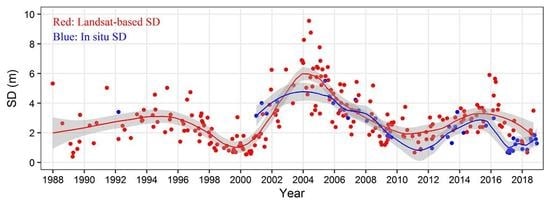
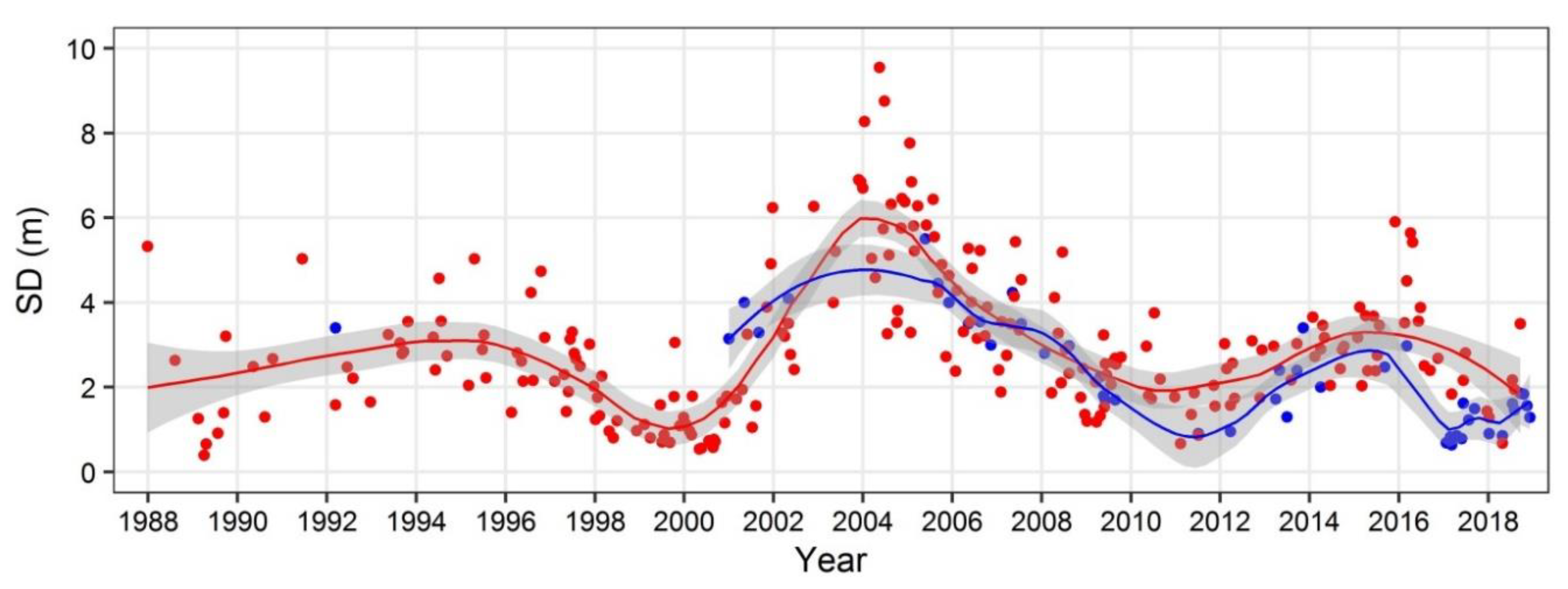
3.3. Long-Term SD Changes in Lake Maninjau from the Landsat TM/ETM+ Time Series

We applied the BF model to the preprocessed Landsat Dataset II to observe the long-term SD change in Lake Maninjau (1987–2018). To maintain the representativeness of the SD of the entire lake, we excluded Landsat images with <50% available water pixels in Lake Maninjau (see Section 2.3.1 above). We also removed two Landsat images (acquired on 2 July 2004 and 5 July 2005) due to a large area of clouds and cloud shadows that failed to be masked by the BQA, NDWI, and MNDWI values. Only 230 Landsat images were thus used for the long-term SD change analysis.

Figure 5 provides the averaged SD values estimated from the 230 preprocessed Landsat images using the BF model. The averaged in situ SD measurements of each field survey in Lake Maninjau are also shown in the figure for visual comparison. From the long-term Landsat-based SD estimations, we can see that low SD values (1–1.5 m) occurred four times during the years from 2001 to 2018 (around 1989, 1999, 2011, and 2018). Around 2004, the water transparency in Lake Maninjau increased notably, as the SD values changed from 1.5 m (around 1999) to approximately 6 m. The water transparency in the lake then showed a continuous decrease until 2011, a smaller tendency to increase in 2011–2015, and a decreasing trend again in 2015–2018. These water transparency variations observed from the Landsat-based SD estimations can be validated by the In Situ SD Dataset II after 2001 (Figure 5, blue points and trend line), which showed a similar fluctuation pattern of SD values.

4. Discussion

4.1. The Applicability of the Developed SD Estimation Model

We developed an empirical model for estimating SD values from Landsat data. Although the number of data pairs is small, the pairs were collected from nine Indonesian lakes with a wide dynamic range of SD values (0.5–18.6 m). We also conducted a series of preprocessing steps, including the removal of contaminated water pixels, the filtering of the images, and the mitigation of the atmospheric effects, before the Landsat data were used. These efforts enable the developed SD estimation model to be applied to different Landsat images cross time and space [6,28,29]. In contrast, since the fewer available bands and the broad bandwidths of Landsat TM and ETM+ sensors, the changed IOPs in different waterbodies are probably not the main cause to affect the robustness and universality of the developed SD estimation model. Nevertheless, the developed SD estimation model still needs to be further validated by using more comprehensive data pairs collected from various waters or simulation experiments.

Many researchers have suggested the use of the band ratio of TM1/TM3 and the single band of TM1 as an SD predictor (i.e., the A1 model in Table 4; e.g., [6,7,12,26,27,28,29]). This suggestion differs from the recommendation of our present investigation, which used the two band ratios of TM1/TM2 and TM3/TM2 as independent variables in the SD estimation model (i.e., the BF model in Table 4). The A1 model showed the best performance in the calibration procedure, with the highest R² value of 0.99 and the smallest RMSE of 0.8 m (Figure 2b). However, the A1 model showed a lower R² value (0.34) and larger error (RMSE = 2.0 m) in the validation procedure (Figure 3b). We also observed many outliers in the SD estimations when the A1 model was applied to the Landsat Dataset II to estimate long-term SD changes (data not shown). Similar results were observed in all of the A-type and B-type models (Figure 2 and Figure 3). These findings indicate that the A-type models present large uncertainty, whereas the B-type models are more robust in many applications.

Another difference between the current model and previous models is that we used the band ratio instead of a single band for the second independent variable (i.e., we used TM3/TM2 instead of TM1). The merit of using the band ratio is that effects due to imperfect atmospheric correction can be mitigated [59,60]. In addition, since water-leaving reflectance at the green band (TM2) does not change as much as that at the blue and red bands (TM1 and TM3) in various waters, using this value to normalize water-leaving reflectance at blue and red bands can avoid a large fluctuation of the ratios. The BF model thus showed the greatest robustness in Lake Maninjau.

4.2. The Reliability of the Estimated SD Values from Landsat Data

Febrianti in 2000 [61] and Sulastri in 2002 [62] reported that a heavy algal bloom occurred in 2000 in Lake Maninjau. This event was also detected by our Landsat-based SD estimations, which showed low SD values during that period (Figure 5). To weaken the algal bloom effects on Lake Maninjau, local residents around the lake asked the power company to open the secondary water gate in March 2001 to flush the surface waters [31,50]. Since then, the water transparency in Lake Maninjau has increased significantly. The RCL (LIPI) observed the highest SD values of 4.1 m in May 2002 and 5.8 m in May 2005 [63]. The trend of increased water transparency was also revealed by the time-series Landsat data (Figure 5). These results indicate that water level management is effective to improve water quality.

The continuous decrease in the SD values revealed during period from 2004 to 2012 by both the in situ-measured and Landsat-based SD values can be explained by the dramatically increased number of fish cages in Lake Maninjau. In 2005, the number of fish cages in the lake was 4920 units, and this number increased to 8955 units in 2006 and 13,129 units in 2010 (Figure 1d). We observed a strong correlation between the number of fish cages and the Landsat-based SD values during the period 2004–2012 (R² = 0.88; Figure 6). This result indicates that the number of fish cages in Lake Maninjau is probably a major driving factor of water transparency in the lake.

Overall, the Landsat-based SD estimations well captured the changes in water transparency in Lake Maninjau, and these estimations can therefore provide useful data for lake managers and policy-makers. It should also be noted that the tendency of long-term change in the SD from historical Landsat images is more reliable than a single SD estimation.

5. Conclusions

We developed an empirical model to estimate SD values from Landsat TM/ETM+ data. The developed model suggests the use of the two band ratios of TM1/TM2 and TM3/TM2 as the SD predictor to reduce uncertainties in the model. This suggestion differs from the recommendations in previous studies. The preprocessing procedure for Landsat data is important for improving the robustness of the developed model. Our determination of the estimated long-term SD time series in Lake Maninjau indicates that the Landsat data, along with the developed model, can be used to generate a long-term SD database to monitor water transparency changes in Indonesian inland waters.

References

1. Sulastri. Inland water resources and limnology in Indonesia. Tropics 2006, 15, 285–295. Available online: https://www.jstage.jst.go.jp/article/tropics/15/3/15_3_285/_pdf/-char/en (accessed on 19 April 2018). [CrossRef]
2. Ministry of Environment of the Republic of Indonesia. Profil 15 Danau Prioritas Nasional; Kementerian Lingkungan Hidup Republik Indonesia: Jakarta, Indonesia, 2011; pp. 1–148. [Google Scholar]
3. Ruttner, F. Hydrographische und Hydrochemishe Beobachtungen auf Java, Sumatera und Bali. Arch. Hydrobiol. Suppl. 1930, 8, 197–454. [Google Scholar]
4. Lehmusluoto, P.; Machbub, B.; Terangna, N.; Rusmiputro, S.; Achmad, F.; Boer, L.; Brahmana, S.; Priadi, B.; Setiadji, B.; Sayuman, O.; et al. National Inventory of the Major Lakes and Reservoirs in Indonesia. General Limnology, Revised ed.; Research Institute for Water Resources Development, Ministry of Public Works, Agency for Research and Development: Bandung, Indonesia, 1997; pp. 1–71.
5. Giardino, C.; Pepe, M.; Brivio, P.A.; Ghezzi, P.; Zilioli, E. Detecting chlorophyll, Secchi disk depth and surface temperature in a sub-alpine lake using Landsat imagery. Sci. Total Environ. 2001, 268, 19–29. [Google Scholar] [CrossRef]
6. Kloiber, S.M.; Brezonik, P.L.; Bauer, M.E. Application of Landsat imagery to regional-scale assessment of lake clarity. Water Res. 2002, 26, 4330–4340. [Google Scholar] [CrossRef]
7. Olmanson, L.G.; Bauer, M.E.; Brezonik, P.L. A 20-year Landsat water clarity census of Minnesota’s 10,000 Lakes. Remote Sens. Environ. 2008, 112, 4086–4097. [Google Scholar] [CrossRef]
8. Olmanson, L.G.; Brezonik, P.L.; Bauer, M.E. Evaluation of medium to low resolution satellite imagery for regional lake water quality assessments. Water Resour. Res. 2011, 47, W09515. [Google Scholar] [CrossRef] [Green Version]
9. Bonansea, M.; Ledesma, C.; Rodríguez, C.; Pinotti, L.; Antunes, H.M. Effects of atmospheric correction of Landsat imagery on lake water clarity assessment. Adv. Space Res. 2015, 56, 2345–2355. [Google Scholar] [CrossRef]
10. Dörnhöfer, K.; Oppelt, N. Remote sensing for lake research and monitoring. Recent Adv. Ecol. Indic. 2016, 64, 105–122. [Google Scholar] [CrossRef]
11. Gholizadeh, M.H.; Melesse, A.M.; Reddi, L. A Comprehensive Review on Water Quality Parameters Estimation Using Remote Sensing Techniques. Sensors 2016, 16, 1298. [Google Scholar] [CrossRef] [Green Version]
12. Olmanson, L.G.; Brezonik, P.L.; Finlay, J.C.; Bauer, M.E. Comparison of Landsat 8 and Landsat 7 for regional measurements of CDOM and water clarity in lakes. Remote Sens. Environ. 2016, 185, 119–128. [Google Scholar] [CrossRef]
13. Blondeau-Patissier, D.; Gower, J.F.; Dekker, A.G.; Phinn, S.R.; Brando, V.E. A review of ocean color remote sensing methods and statistical techniques for the detection, mapping and analysis of phytoplankton blooms in coastal and open oceans. Prog. Oceanogr. 2014, 123, 123–144. [Google Scholar] [CrossRef] [Green Version]
14. Oyama, Y.; Matsushita, B.; Fukushima, T.; Matsushige, K.; Imai, A. Application of spectral decomposition algorithm for mapping water quality in a turbid lake (Lake Kasumigaura, Japan) from Landsat TM data. ISPRS J. Photogramm. Remote Sens. 2009, 64, 73–85. [Google Scholar] [CrossRef]
15. Kutser, T. The possibility of using the Landsat image archive for monitoring long time trends in coloured dissolved organic matter concentration in lake waters. Remote Sens. Environ. 2012, 123, 334–338. [Google Scholar] [CrossRef]
16. Zheng, Z.; Li, Y.; Guo, Y.; Xu, Y.; Liu, G.; Du, C. Landsat-Based Long-Term Monitoring of Total Suspended Matter Concentration Pattern Change in the Wet Season for Dongting Lake, China. Remote Sens. 2015, 7, 13975–13999. [Google Scholar] [CrossRef] [Green Version]
17. Lobo, F.L.; Costa, M.P.F.; Novo, E.M.L.M. Time-series analysis of Landsat-MSS/TM/OLI images over Amazonian waters impacted by gold mining activities. Remote Sens. Environ. 2015, 157, 170–184. [Google Scholar] [CrossRef]
18. Lee, Z.; Shang, S.; Qi, L.; Yan, J.; Lin, G. A semi-analytical scheme to estimate Secchi-disk depth from Landsat-8 measurements. Remote Sens. Environ. 2016, 177, 101–106. [Google Scholar] [CrossRef]
19. Rodrigues, T.; Alcantara, E.; Watanabe, F.; Imai, N. Retrieval of Secchi disk depth from a reservoir using a semi-analytical scheme. Remote Sens. Environ. 2017, 198, 213–228. [Google Scholar] [CrossRef] [Green Version]
20. Lee, Z.; Shang, S.; Hu, C.; Du, K.; Weidemann, A.; Hou, W.; Lin, J.; Lin, G. Secchi disk depth: A new theory and mechanistic model for underwater visibility. Remote Sens. Environ. 2015, 169, 139–149. [Google Scholar] [CrossRef] [Green Version]
21. Lee, Z.; Carder, K.L.; Arnone, R.A. Deriving inherent optical properties from water color: A multiband quasi-analytical algorithm for optically deep waters. Appl. Opt. 2002, 41, 5755–5772. [Google Scholar] [CrossRef]
22. Yang, W.; Matsushita, B.; Chen, J.; Yoshimura, K.; Fukushima, T. Retrieval of inherent optical properties for turbid inland waters from remote-sensing reflectance. IEEE Trans. Geosci. Remote Sens. 2013, 51, 3761–3773. [Google Scholar] [CrossRef]
23. Lathrop, R.G. Landsat thematic mapper monitoring of turbid inland water quality. Photogramm. Eng. Remote Sens. 1992, 58, 465–470. [Google Scholar]
24. Lavery, P.; Pattiaratchi, C.; Wyllie, A.; Hick, P. Water quality monitoring in estuarine waters using the Landsat thematic mapper. Remote Sens. Environ. 1993, 46, 268–280. [Google Scholar] [CrossRef]
25. Cox, R.M.; Forsythe, R.D.; Vaughan, G.E.; Olmsted, L.L. Assessing water quality in the Catawba river reservoirs using Landsat thematic mapper satellite data. Lake Reserv. Manag. 1998, 14, 405–416. [Google Scholar] [CrossRef]
26. Brezonik, P.; Menken, K.D.; Bauer, M. Landsat-based Remote Sensing of Lake Water Quality Characteristics, Including Chlorophyll and Colored Dissolved Organic Matter (CDOM). Lake Reserv. Manag. 2005, 21, 373–382. [Google Scholar] [CrossRef]
27. Zhao, D.; Cai, Y.; Jiang, H.; Xu, D.; Zhang, W.; An, S. Estimation of water clarity in Taihu Lake and surrounding rivers using Landsat imagery. Adv. Water Resour. 2011, 34, 165–173. [Google Scholar] [CrossRef]
28. Sriwongsitanon, N.; Surakit, K.; Thianpopirug, S. Influence of atmospheric correction and number of sampling points on the accuracy of water clarity assessment using remote sensing application. J. Hydrol. 2011, 401, 203–220. [Google Scholar] [CrossRef]
29. Bonansea, M.; Rodríguez, C.; Pinotti, L.; Ferrero, S. Using multi-temporal Landsat imagery and Linear mixed models for assessing water quality parameters in Rio Tercero reservoir (Argentina). Remote Sens. Environ. 2015, 158, 28–41. [Google Scholar] [CrossRef]
30. Butt, M.J.; Nazeer, M. Landsat ETM+ Secchi Disc Transparency (SDT) retrievals for Rawal Lake, Pakistan. Adv. Space Res. 2015, 56, 1428–1440. [Google Scholar] [CrossRef]
31. Nichol, J.E.; Vohora, V. Noise over water surface in Landsat TM images. Int. J. Remote Sens. 2004, 25, 2087–2094. [Google Scholar] [CrossRef]
32. Fakhrudin, M.; Wibowo, H.; Subehi, L.; Ridwansyah, I. Karakterisasi Hidrologi Danau Maninjau Sumatera Barat. In Proceedings of the Seminar Nasional Limnologi 2002, Bogor, Indonesia, 22 April 2002; Pusat Penelitian Limnologi—LIPI: Bogor, Indonesia, 2002; pp. 65–75. [Google Scholar]
33. Syandri, H. Loading and Distribution of Organic Materials in Maninjau Lake West Sumatra Province-Indonesia. J. Aquac. Res. Dev. 2014, 5, 1–4. [Google Scholar] [CrossRef] [Green Version]
34. Badan Pusat Statistik Kabupaten Agam. Agam in Figures 2015. Available online: https://agamkab.bps.go.id/publication/2016/01/27/9e1bdfeacc59787c00e6a53e/kabupaten-agam-dalam-angka-2015.html (accessed on 15 February 2019).
35. Badan Pusat Statistik Kabupaten Agam. Agam in Figures 2016. Available online: https://agamkab.bps.go.id/publication/2016/07/15/3a4ed5ae43c41906b939bf50/kabupaten-agam-dalam-angka-2016.html (accessed on 15 February 2019).
36. Badan Pusat Statistik Kabupaten Agam. Agam in Figures 2017. Available online: https://agamkab.bps.go.id/publication/2017/08/11/2ef8e1564e24faf29cd9ebd4/kabupaten-agam-dalam-angka-2017.html (accessed on 15 February 2019).
37. Badan Pusat Statistik Kabupaten Agam. Agam in Figures 2018. Available online: https://agamkab.bps.go.id/publication/2018/08/16/61f234670dec4ca6f38c0024/kabupaten-agam-dalam-angka-2018.html (accessed on 15 February 2019).
38. Ridwansyah, I.; Subehi, L.; Yulianti, M.; Triwisesa, E.; Nasahara, K. Impact of LULC Change on Hydrological Response in Lake Maninjau Catchment Area. In Proceedings of the 17th World Lake Conference, Lake Kasumigaura, Ibaraki, Japan, 15–19 October 2018; pp. 289–291. [Google Scholar]
39. Landsat Science—Landsat 5. Available online: https://landsat.gsfc.nasa.gov/landsat-5/ (accessed on 16 April 2018).
40. Landsat Science—Landsat 7. Available online: https://landsat.gsfc.nasa.gov/landsat-7/ (accessed on 16 April 2018).
41. USGS Earth Explorer. Available online: https://earthexplorer.usgs.gov/ (accessed on 11 March 2019).
42. McFeeters, S.K. The use of normalized difference water index (NDWI) in the delineation of open water features. Int. J. Remote Sens. 1996, 17, 1425–1432. [Google Scholar] [CrossRef]
43. Xu, H. Modification of normalized difference water index (NDWI) to enhance open water features in remotely sensed imagery. Int. J. Remote Sens. 2006, 27, 3025–3033. [Google Scholar] [CrossRef]
44. Poros, D.J.; Petersen, C.J. A method for destriping Landsat Thematic Mapper images: A feasibility study for an online destriping process in the Thematic Mapper image processing System (TIPS). Photogramm. Eng. Remote Sens. 1985, 51, 1371–1378. [Google Scholar]
45. Chander, G.; Markham, B.; Dennis, D.L. Summary of current radiometric calibration coefficients for Landsat MSS, TM, ETM+, and EO-1 ALI sensors. Remote Sens. Environ. 2009, 113, 893–903. [Google Scholar] [CrossRef]
46. Wang, S.; Li, J.; Zhang, B.; Spyrakos, E.; Tyler, A.N.; Shen, Q.; Zhang, F.; Kuster, T.; Lehmann, M.K.; Wu, Y.; et al. Trophic state assessment of global inland waters using a MODIS-derived Forel-Ule index. Remote Sens. Environ. 2018, 217, 444–460. [Google Scholar] [CrossRef] [Green Version]
47. Vermote, E.F.; Tanré, D.; Deuzé, J.L.; Herman, M.; Morcrette, J.L. Second Simulation of the Satellite Signal in the Solar Spectrum, 6S: An Overview. IEEE Trans. Geosci. Remote Sens. 1997, 35, 675–686. [Google Scholar] [CrossRef] [Green Version]
48. Feng, L.; Hou, X.; Li, J.; Zheng, Y. Exploring the potential of Rayleigh-corrected reflectance in coastal and inland water applications: A simple aerosol correction method and its merits. ISPRS J. Photogramm. Remote Sens. 2018, 146, 52–64. [Google Scholar] [CrossRef]
49. R Core Team. R: A language and environment for statistical computing. In R Foundation for Statistical Computing; Vienna, Austria, 2018; Available online: https://www.R-project.org/ (accessed on 5 March 2019).
50. Zambrano-Bigiarini, M. hydroGOF: Goodness-of-fit functions for comparison of simulated and observed hydrological time series. In R Package Version 0.3-10; 2017; Available online: http://hzambran.github.io/hydroGOF/ (accessed on 15 November 2019). [CrossRef]
51. Willmott, C.J. On the Validation of Models. Phys. Geogr. 1981, 2, 184–194. [Google Scholar] [CrossRef]
52. Nash, J.E.; Sutcliffe, J.V. River Flow Forecasting Through Conceptual Models Part I: A Discussion of Prinicples. J. Hydrol. 1970, 10, 282–290. [Google Scholar] [CrossRef]
53. Carslaw, D.C.; Ropkins, K. Openair—An R package for air quality data analysis. Environ. Model. Softw. 2012, 27–28, 52–61. [Google Scholar] [CrossRef]
54. Taylor, K.E. Summarizing multiple aspect of model performance in a single diagram. J. Geophys. Res. Atmos. 2001, 106, 7183–7192. [Google Scholar] [CrossRef]
55. Wickham, H. Ggplot2: Elegant Graphics for Data Analysis; Springer: New York, NY, USA, 2016. [Google Scholar]
56. Cristina, S.; Cordeiro, C.; Lavender, S.; Costa Goela, P.; Icely, J.; Newton, A. MERIS phytoplankton time series products from the SW Iberian Peninsula (Sagres) using seasonal-trend decomposition based on loess. Remote Sens. 2016, 8, 449. [Google Scholar] [CrossRef] [Green Version]
57. Lu, H.; Raupach, M.R.; McVicar, T.R.; Barrett, D.J. Decomposition of vegetation cover into woody and herbaceous components using AVHRR NDVI time series. Remote Sens. Environ. 2003, 86, 1–18. [Google Scholar] [CrossRef]
58. Jiang, B.; Liang, S.; Wang, J.; Xiao, Z. Modeling MODIS LAI time series using three statistical methods. Remote Sens. Environ. 2010, 114, 1432–1444. [Google Scholar] [CrossRef]
59. Doxaran, D.; Froidefond, J.M.; Castaing, P. A reflectance band ratio used to estimate suspended matter concentrations in sediment-dominated coastal waters. Int. J. Remote Sens. 2002, 23, 5079–5085. [Google Scholar] [CrossRef]
60. Doxaran, D.; Froidefond, J.M.; Castaing, P. Remote-sensing reflectance of turbid sediment-dominated waters. Reduction of sediment type variations and changing illumination conditions effects by use of reflectance ratios. Appl. Opt. 2003, 42, 2623–2634. [Google Scholar] [CrossRef]
61. Febrianti. Attack of the Algae at Lake Maninjau. Tempo: Indonesia's Weekly News Magazine. 19 November 2000. Available online: https://search.proquest.com/docview/198798412?accountid=25225 (accessed on 20 February 2019).
62. Sulastri. Spatial and Temporal Distribution of Phytoplankton in Lake Maninjau, West Sumatera. In Proceedings of the International Symposium on Land Management and Biodiversity in South East Asia, Bali, Indonesia, 17–20 September 2002; pp. 403–408. [Google Scholar]
63. Henny, C.; Nomosatryo, S. Changes in water quality and trophic status associated with aquaculture in Lake Maninjau, Indonesia. IOP Conf. Ser. Earth Environ. Sci. 2016, 31, 012027. [Google Scholar] [CrossRef] [Green Version]
Figure 1. (a) Landsat image of Lake Maninjau in Sumatera Island, Indonesia (acquired on 6 July 2011; R:G:B = 4:5:1; green stars = the measurement sites). (b) Locations of the nine Indonesian lakes investigated in 2011–2014 and used for calibrating the Secchi disk depth (SD) estimation model (green circles). (c) Monthly averaged precipitation of Lake Maninjau [32]. (d) Number of fish cages and fish production in Lake Maninjau from 1992 to 2016 [33,34,35,36,37].
Remotesensing 11 02875 g001
Figure 2. Comparison of the in situ SD measurements and the corresponding estimated SD values using the 17 selected models in the model calibration procedures.
Remotesensing 11 02875 g002
Figure 3. Comparisons of the in situ-measured SD values (In Situ SD Dataset III) and the corresponding estimated SD values from the preprocessed Landsat images (Landsat Dataset III) using the 17 selected SD estimation models (n = 74).
Remotesensing 11 02875 g003
Figure 4. Comparison of the 17 selected SD estimation models using Taylor diagram in terms of their correlation coefficients, root-mean-square differences, and standard deviations.
Remotesensing 11 02875 g004
Figure 5. Long-term changes in the water transparency in Lake Maninjau from 1987 to 2018. Red points: The averaged SD values estimated from the preprocessed Landsat Dataset II using the BF model. Blue points: The averaged in situ SD values for each field survey (In Situ SD Dataset II). Red line: Obtained from the red points via a trend analysis in R language. Blue line: Obtained from the blue points via a trend analysis in R language. Gray areas: 95% confidence intervals of the trend analysis.
Remotesensing 11 02875 g005
Figure 6. Relationship between the number of fish cages and the Landsat-based SD values during the period 2004–2012 in Lake Maninjau (n = 9).
Remotesensing 11 02875 g006