Biomass Estimation for Semiarid Vegetation and Mine Rehabilitation Using Worldview-3 and Sentinel-1 SAR Imagery

Abstract

The surface mining activities in grassland and rangeland zones directly affect the livestock production, forage quality, and regional grassland resources. Mine rehabilitation is necessary for accelerating the recovery of the grassland ecosystem. In this work, we investigate the integration of data obtained via a synthetic aperture radar (Sentinel-1 SAR) with data obtained by optical remote sensing (Worldview-3, WV-3) in order to monitor the conditions of a vegetation area rehabilitated after coal mining in North China. The above-ground biomass (AGB) is used as an indicator of the rehabilitated vegetation conditions and the success of mine rehabilitation. The wavelet principal component analysis is used for the fusion of the WV-3 and Sentinel-1 SAR images. Furthermore, a multiple linear regression model is applied based on the relationship between the remote sensing features and the AGB field measurements. Our results show that WV-3 enhanced vegetation indices (EVI), mean texture from band8 (near infrared band2, NIR2), the SAR vertical and horizon (VH) polarization, and band 8 (NIR2) from the fused image have higher correlation coefficient value with the field-measured AGB. The proposed AGB estimation model combining WV-3 and Sentinel 1A SAR imagery yields higher model accuracy (R² = 0.79 and RMSE = 22.82 g/m²) compared to that obtained with any of the two datasets only. Besides improving AGB estimation, the proposed model can also reduce the uncertainty range by 7 g m⁻² on average. These results demonstrate the potential of new multispectral high-resolution datasets, such as Sentinel-1 SAR and Worldview-3, in providing timely and accurate AGB estimation for mine rehabilitation planning and management.

1. Introduction

Several large surface mining sites are located in North China, especially in the semiarid grassland of Inner Mongolia. The mining, extraction, and processing of mineral resources (particularly ores) from such sites require full aggressive removal of the on-site vegetation, surface soil, and bedrock. The removal of these natural environmental ingredients leads to a significant degradation in the grassland ecosystems [1]. One of the principal rehabilitation techniques employed to remedy the resulting environmental problems and restore the ecological functions is the re-establishment of the vegetation in the mining sites [2]. Vegetation mapping provides critical information for the understanding and assessment of rehabilitation processes in mining sites. One of the most essential carbon pool indicators in mine rehabilitation ecosystems is the above-ground biomass (AGB). Timely and accurate biomass assessment and mapping is crucial for reclaiming mining sites in semiarid grasslands. However, biomass measurements are quite costly and infeasible for large areas. Estimation models, which are based on the correlation between field biomass data and spectral, texture, and polarization information from remote sensing imagery, can be applied for timely and effective AGB monitoring across large area [3].

Common tools for mining site reclamation include optical multispectral sensors, satellite imagery, and hyperspectral data. For example, these tools are used in land change detection [4], vegetation health assessment [2], and soil property prediction [5]. However, the use of optical sensors for the AGB estimation in semiarid mining locations is limited by the vegetation structure as well as the saturation of the high-vegetation cover [6]. Vegetation monitoring can be carried out with synthetic aperture radar (SAR) sensors, because of the sensitivity of these sensors to the geometrical and dielectric plant characteristics, and their superior imaging outcomes compared to optical images [7]. Combining SAR and optical sensors can help in differentiating between vegetation classes and improving the mapping accuracy [8,9]. Combination schemes can be formed in two ways: incorporating all sensor data as extra bands, or the fusion of the optical and SAR data with a fusion algorithm, such as the wavelet principal component analysis [10]. For mined lands of regional extents, optical high-resolution spatial and spectral remote sensing data is required for deriving detailed surface material information [11,12]. The Worldview-3 data has relatively higher spatial and spectral resolutions, and is characterized by sensitivity and surface reflectance variations that can help in distinguishing vegetation types [13]. SAR imagery has not been widely used in biomass mapping and mine rehabilitation due to its limited area coverage and high acquisition cost. New opportunities for mapping vegetation emerged with the recent launch of Sentinel-1 as a joint initiative of the European Commission (EC) and the European Space Agency (ESA) and the release of the collected SAR data [8]. Moreover, mine reclamation can be further improved by exploiting the complementarity between the SAR and optical multispectral imagery.

In this paper, we investigate the combination of the data from Sentinel-1 SAR and Worldview-3 (WV-3) imagery for mapping the biomass of reclaimed vegetation in mined environments. Specifically, the aims of this work are to (1) create a model of the relationship between the AGB field measurements and each of the Sentinel-1 SAR backscatter coefficients and the WV-3 multispectral reflectance measurements; (2) assess the potential of the fused SAR and WV-3 data for improving the biomass estimation accuracy; (3) evaluate the spatial distribution and the uncertainty of the output biomass maps. In a nutshell, this paper is an attempt towards the development of remote sensing techniques using Sentinel-1 SAR data and WV-3 optical data for biomass modeling and mapping to support mine reclamation.

2. Materials and Methods

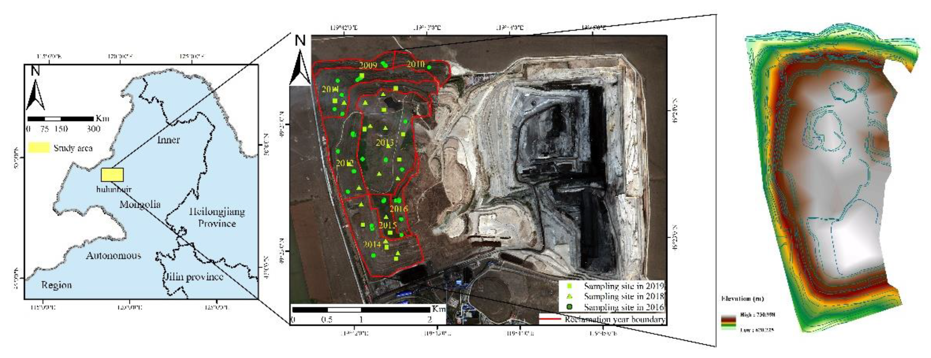
2.1. Field Study Location

The Baori Hiller Surface Coal Mine (BHCM) is located in the center of the Hulun Buir meadow steppe in North China, as seen in Figure 1. This mining site has been active since 2004, and its reclamation began in 2009. Our study area is the BHCM reclaimed dump. The dump has a stepped design with a maximum step height of 20 m, a main step gradient of 18%, and a platform height of 100 m. Because it was formed by piling waste soil and rocks throughout the mining process, the topography is significantly different from the original natural topography with several platforms and slope, as seen in Figure 1. This dump was covered with over 20 cm of natural topsoil of Kastanozems to support natural vegetation and to act as a growth medium for accelerated artificial revegetation. The main plant species on the flat part of the reclaimed dump are Elymus dahuricus Turcz., Medicago falcata L., Artemisia sieversiana Ehrhart ex Willd., Salsola collina Pall., Scutellaria baicalensis Georgi., see

Table 1. A chronological summary of the mine rehabilitation progress.

Reclamation Year	Vegetation Cover	Dominant Species	Number of Sampling Sites
			2016	2018	2019
2009	50%	Elymus dahuricus Turcz.	3	0	0
		Heteropappus altaicus (Willd.) Novopokr.
2010	50%	Elymus dahuricus Turcz.	2	0	0
2011	60%	Elymus dahuricus Turcz.	6	2	1
		Artemisia sieversiana
2012	62%	Artemisia sieversiana	6	1	2
		Scutellaria baicalensis Georgi
		Bupleurum chinensis DC.
2013	70%	Medicago falcata L.	4	4	4
2014	57%	Elymus dahuricus Turcz.	4	3	3
2015	75%	Medicago falcata L.	3	1	2
2016	50%	Elymus dahuricus Turcz.	4	1	2

.

A field survey was conducted in the platform of the dump from the 1st to the 7th of August 2016, 25 to 29 July 2018, and 20 to 26 July 2019, when no extreme weather conditions occurred. The land cover was classified into eight subregions with different reclamation year, as seen in Table 1, Figure 1. Normally, within a rehabilitation year, the rehabilitation project, including topsoil properties and planting species, is similar. The samples we selected were assigned within the subregion using grid numbers according to a stratified, random sampling method. Such a design provided randomness and helped to avoid uneven distribution of sample points. This approach assigns a specific number of sample sites to each subregion in proportion to the size or significance of the subregion according to the project objectives. At each sampling site, three plots with size of 0.5 m × 0.5 m were selected. Digital images were captured from each measuring plot. The plant coverage for a given plots was derived as the greenness value of the captured image. AGB measurements were collected by destructive sampling from each plot. Fresh samples were collected, dried at 70 °C for 72 h, and then weighed to obtain the total AGB. The average AGB of three plots was calculated for each sampling site. In total, field-measured AGB from 32 sampling sites at 2016 were collected and used to estimate AGB based on remote sensing data, where the remote sensing data was collected at the same period. Additionally, in order to justify the methodology, field-measured AGB of 12 sampling sites in 2018 and field-measured AGB of 14 sampling sites were collected in 2019.

2.2. Satellite Data Collection

In this work, the optical data used is Worldview-3 (WV-3) multispectral data acquired on the 11 of August 2016.

Table 2. Spatial, temporal, and spectral characteristics of the Worldview-3 (WV-3) remote sensor.

Sensor	Spatial Resolution	Band Name	Wavelength (nm)
		Coastline	400–450
		Blue	450–510
		Green	510–580
Worldview-3	1.24 m	Yellow	585–625
		Red	630–690
		Red edge	705–745
		NIR1	770–895
		NIR2	860–1040

summarizes the spatial, temporal, and spectral characteristics of the associated sensor. Preprocessing operations of the WV-3 data are geometric correction, radiometric calibration, and FLAASH atmospheric correction by ENVI5.3. The available Sentienl-1A data around field survey period (1–7 August 2016) were downloaded from the Sentinel data hub. Finally, there were four images used in this study, as seen in

Table 3. Characteristics of Sentienl-1A images used.

Acquisition Time	Polarization Mode	Radiation Precision	Resolution
29 July 2016	VV+VH		20 m (Azimuth resolution)
5 August 2016
10 August 2016			5 m (Range resolution)
17 August 2016

.

2.3. Image Preprocessing

2.3.1. Synthetic Aperture Radar Image Preprocessing

Three preprocessing procedures were applied to each scene prior to image reconstruction and image fusion, as seen in Figure 2. These are radiometric correction, lee filtering, and terrain correction. ESA’s Sentinel Application Platform (SNAP) software was used for the preprocessing. Radiometric calibration was conducted so that the pixel values truly represent the radar backscatter of the reflecting surface. The backscatter values were eventually converted to decibels using Equation (1). The backscattering coefficient unit is dB.

$$\mathrm{Backscattering}\mathrm{coefficient}=10\times {{\displaystyle \log }}_{10}\mathrm{intensity}$$

(1)

Speckle noise, due to constructive and deconstructive wave interference in the image, was minimized using the Refined Lee filter method, which was selected due to its reported superior performance in SNAP [14]. Shuttle Radar Topography Mission (SRTM) Digital Elevation Model (DEM) at 30 m resolution and 1 m DEM covering the study area derived from airborne photogrammetry in 2014 were combined for terrain correction. Specifically, the 30 m SRTM was resampled into pseudo 1 m resolution and data within study area was replaced by the true 1 m DEM. The merged DEM was then used for the terrain correction of SAR image.

2.3.2. SAR Image Reconstruction

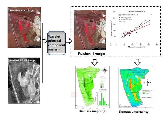
Super-resolution image reconstruction seeks to construct a high-resolution image from multiple low-resolution ones for better visual effects [15]. The projection-over-convex-set (POCS) method exploits the projection residue to improve the visual appearance of the reconstructed high-resolution image [16,17]. Notably, this method takes a full advantage of the statistical properties of the projection residue included in the constraints and adaptively changes the modified threshold. In this work, SAR images were reconstructed by using four Sentinel-1A SAR images to improve the image-based discrimination capability, and to increase the detail using the four acquired images based on the POCS algorithm.

The signal-to-noise ratio (SNR) is computed from the local mean and the standard deviation. A larger SNR value represents more image detail. The SNR is computed as follows: (i) find the image average M; (ii) find the local mean and the standard deviation for each image block; (iii) get the mean value of the local standard error (LSD); (iv) compute the SNR as

$$SNR=\frac{M}{LSD}$$

(2)

The reconstructed SAR image was resampling to 1.24 m, corresponding to the spatial resolution of WV-3 imagery. The reconstructed SAR image and WV-3 image were georegistered to each other based on 30 ground control points using cubic convolution sampling method within root mean square error of 0.5 pixels.

2.3.3. Image Fusion

The stronger backscattering from sampling sites was recorded in the vertical and vertical VV polarization data with relatively higher backscatter coefficient value, rather than VH polarization. Therefore, we used VV polarization of the constructed SAR image to fuse with the WV-3 image. The image fusion was conducted by wavelet principal component analysis (W-PCA), which can provide the highest accuracy in land cover classification and vegetation mapping based on the use of optical and SAR data for information extraction [18,19]. The steps of the W-PCA fusion are: (i) apply PCA to the multispectral WV-3 image data and obtain the first principal component (PC1); (ii) match the histograms of the Sentinel-1 and PC1 image data; (ii) utilize a wavelet decomposition to merge Sentinel-1 images into the PC1 image; (iv) apply the inverse PCA transform so that the embedded Sentinel-1 information carried by the PC1 image can be integrated to obtain the fused image.

The fused images can be generally evaluated using data indicators such as the information entropy, the average gradient, the spatial similarity coefficient, and the spectral distortion.

The information entropy represents the amount of information contained in an image. With no excessive noise, the information entropy is richer and the image detail information is better. This entropy is calculated as:

$$H=-{\displaystyle \sum _{i=0}^{M-1}{{\displaystyle p}}_i\lg {{\displaystyle p}}_i}{{\displaystyle p}}_i=\raisebox{1ex}{${{\displaystyle N}}_i$}\!\left/ \!\raisebox{-1ex}{$N$}\right.$$

(3)

where H is the image information entropy, M is the number of image gray levels, $i$ is the number of pixels of the gray value, and N is the total number of pixels in the image.

The average gradient reflects the image sharpness and shows the minute image details of contrast and texture changes. This gradient is given by:

$$\stackrel{-}{G}=\frac{1}{M*N}{\displaystyle \sum _{i=1}^{M-1}{\displaystyle \sum _{j=1}^{N-1}\sqrt{{{\displaystyle ({{\displaystyle \Delta I}}_x^2+{{\displaystyle \Delta I}}_y^2)}}^{/2}}}}$$

(4)

where ${{\displaystyle \Delta I}}_x^2$ and ${{\displaystyle \Delta I}}_y^2$ are the differences in the $\mathrm{x}$ and $\mathrm{y}$ directions, respectively. The larger the average gradient, the better the image texture information. The average gradient is an important indicator of geologically complex images.

The spatial correlation coefficient reflects the spatial correlation between the fused image and the original high-resolution image. A higher spatial correlation coefficient value indicates that the original high-resolution image contains richer texture details. This coefficient is calculated as:

$$r=\frac{{\displaystyle \sum _{i=0}^M{\displaystyle \sum _{j=1}^N({{\displaystyle f}}_A(\mathrm{i},\mathrm{j})-\overline{{{\displaystyle f}}_A})({{\displaystyle f}}_B(\mathrm{i},\mathrm{j})-\overline{{{\displaystyle f}}_B})}}}{\sqrt{{\displaystyle \sum _{i=0}^M{\displaystyle \sum _{j=1}^N{{\displaystyle ({{\displaystyle f}}_A(\mathrm{i},\mathrm{j})-\overline{{{\displaystyle f}}_A})}}^2{\displaystyle \sum _{i=0}^M{\displaystyle \sum _{j=1}^N{{\displaystyle ({{\displaystyle f}}_B(\mathrm{i},\mathrm{j})-\overline{{{\displaystyle f}}_B})}}^2}}}}}}$$

(5)

where M and N are the numbers of image rows and columns, ${{\displaystyle f}}_A(\mathrm{i},\mathrm{j})$ and ${{\displaystyle f}}_B(\mathrm{i},\mathrm{j})$ are respectively the gray values of the fused and original high-resolution images at (i, j), and $\overline{{{\displaystyle f}}_A}$ and $\overline{{{\displaystyle f}}_B}$ are the average gray values of the high-resolution fused and original images, respectively.

The spectral distortion (or twisting) reflects the degree of distortion of the spectral information of the fused image relative to an original multispectral image. This distortion is defined as the average of the absolute values of all pixel differences of the original and fused images. The larger the value of the spectral distortion, the more severe the spectral change of the fused image. This distortion is calculated as:

$${{\displaystyle D}}_{FA}=\frac{1}{MN}{\displaystyle \sum _{i=1}^M{\displaystyle \sum _{j=1}^N(|\mathrm{F}(\mathrm{i},\mathrm{j})-\mathrm{A}(\mathrm{i},\mathrm{j})|)}}$$

(6)

where M and N are respectively the numbers of image rows and columns, while $\mathrm{F}(\mathrm{i},\mathrm{j})$ and $\mathrm{A}(\mathrm{i},\mathrm{j})$ are the gradation values of the fused and source images at (i, j), respectively.

2.3.4. Feature Parameter Extraction

For the WV-3 spectral bands and the VV/VH polarization data of Sentinel-1 SAR, texture features were computed based on grey-level co-occurrence matrices with window sizes of 3 × 3 pixels. These texture features include the mean (ME), the variance (VA), the uniformity (UN), the dissimilarity (DI), the correlation (CR), the homogeneity (HO), and the second moment (SM). In addition, the following vegetation indices were computed from the multispectral data: the normalized difference vegetative index (NDVI); the difference vegetation index (DVI); the ratio vegetation index (RVI); the normalized greenness vegetation index (NGVI); the antiatmosphere vegetation index (ARVI); the enhanced vegetation index (EVI), and the red-edge normalized vegetation index (NDVI705), as seen in

Table 4. Computational forms and advantages of different vegetation indices.

Vegetative Index	Calculation Formula	Advantages	Reference
NDVI		The most widely used vegetation index; the best indicator of vegetation growth and coverage.	Rouse et al., 1974 [20]
DVI		Sensitive to changes in soil background, using areas with early- or mid-vegetation development or low-vegetation coverage.	Richardson and Weigand, 1977 [21]
RVI		Sensitive to lush, high-coverage vegetation, with high RVI values for green vegetation and low RVI values for nonvegetation.	Pearson and Miller, 1972 [22]
NDGI		Tests different forms of vital vegetation.	Gitelson et al., 1996 [23]
ARVI		Reduces the impact of the atmosphere on the vegetation index.	Kanfman and Tanre, 1992 [24]
EVI		Weakens the influence of the soil background.	Liu and Huete, 1995 [25]
		An improved version of the NDVI index that is very sensitive to small changes in vegetation canopy, forest window fragments, and aging changes.	Sims et al., 2002 [26]

.

2.4. Biomass Estimation Methods

The Pearson correlation coefficient was used to find the correlation between the input variables and the field measured above-ground biomass from 2016. Then, the input variables with high significance were selected to establish a biomass estimation model.

The performance of each model is evaluated by calculating the root mean square error (RMSE) and the estimation accuracy,

$$RMSE=\sqrt{\frac{{{\displaystyle {\displaystyle \sum _{i=1}^n({{\displaystyle AGR}}_i-{{\displaystyle AGR}}_i^{\prime })}}}^2}{N}}$$

(7)

$$Ac=(1-\frac{RMSE}{\overline{AGR}})\times 100\%$$

(8)

where ${{\displaystyle AGR}}_i$ is the measured grassland biomass, ${{\displaystyle AGR}}_i^{\prime }$ is the estimated grassland biomass, $n$ is the number of samples, $Ac$ is the estimation accuracy, and $\overline{AGR}$ is the average of the grassland biomass measurements.

The uncertainty caused by variations in the model residuals can be measured by the standard deviation of the residuals. In other words, this uncertainty is quantified by a linear relationship between the standard deviation of residuals and the above-ground biomass. This relationship is given by:

$${{\displaystyle \delta }}_{\epsilon }=\alpha \overline{\overline{B}}$$

(9)

where ${{\displaystyle \delta }}_{\epsilon }$ is the standard deviation of the residuals, $\alpha$ is the fitted parameter, and $\overline{\overline{B}}$ is the predicted value of the biomass.

3. Results

3.1. Image Reconstruction and Fusion

As shown in Figure 3 and Figure 4, the Sentinel-1 SAR image has been improved after super-resolution reconstruction, in which more details appear and the discriminative capability is improved. The SNR value increased from 5.8 dB before construction to 6.8 dB after construction for the VV polarization image, and from 6.4 dB before construction to 7.9 dB after construction for the VH polarization image.

As shown in Figure 5, the sharpness as well as the spectral and structural texture features of the fused image are visually better than those of a single optical or SAR image. The higher entropy value reflects that more details are present in the fused image compared to the optical WV-3 image. Also, the higher average gradient indicates that the sharpness and texture information of the fused image are better than those of the SAR image, as seen in Figure 6 and Figure 7. Bands 7 and 8 of the fused image generated higher similarity coefficients and lower spectral distortion values in comparison to the WV-3 multispectra image, which shows more texture features and less spectral changes, as seen in Figure 8.

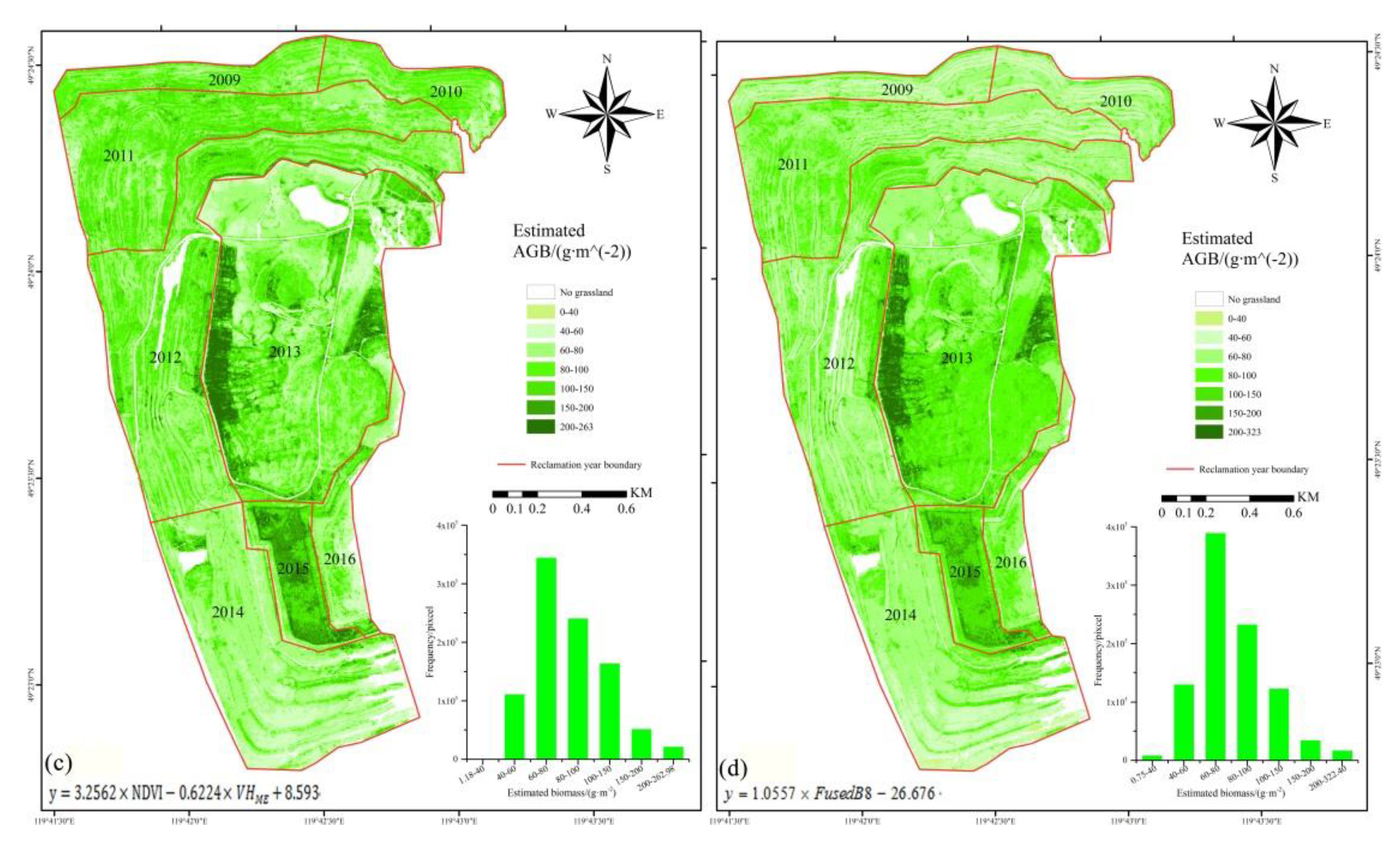
3.2. Above Ground Biomass (AGB)AGB Estimation Models and Uncertainty

Table 5. Correlation analysis between the biomass field measurements and image features.

Worldview-3				Sentinel-1 SAR		Fusion
Spectral Information		Texture Information		Texture Information		Spectral Information
Variable	Correlation	Variable	Correlation	Variable	Correlation	Variable	Correlation
Coastline (B1)	−0.323	B4ME	−0.741 **	VH	0.504 **	B1	−0.759 **
Blue (B2)	−0.474 *	B5ME	−0.792 **	VV	0.410 *	B2	−0.806 **
Green (B3)	−0.372	B5CR	−0.358 *	VVME	0.412 **	B3	−0.837 **
Yellow (B4)	−0.620 **	B6ME	0.511 **	VVVA	0.174	B4	−0.834 **
Red (B5)	−0.657 **	B6CR	−0.412 *	VVHO	−0.238	B5	−0.800 **
Red edge (B6)	0.215	B7ME	0.760 **	VVCO	0.165	B6	0.564 **
NIR1 (B7)	0.694 **	B7VA	0.700 **	VVDI	0.201	B7	0.842 **
NIR2 (B8)	0.718 **	B7HO	−0.593 **	VVEN	0.257	B8	0.874 **
RVI	0.790 **	B7DI	0.535 *	VVSM	−0.219
NGVI	0.871 **	B7EN	0.510 **	VVCR	0.169
NDVI705	0.835 **	B7SM	−0.366 *	VHME	0.503 **
NDVI	0.874 **	B8ME	0.748 **	VHVA	−0.061
EVI	0.876 **	B8VA	0.669 **	VHHO	0.069
DVI	0.833 **	B8HO	−0.600 **	VHCO	0.064
		B8DI	0.558 **	VHDI	−0.016
		B8EN	0.612 **	VHEN	−0.133
		B8SM	0.520 **	VHSM	0.298
				VHCR	−0.195

** Significant correlation at the 0.01 level. * Significant correlation at the 0.05 level.

shows the results of correlation analysis between image features and the field measured biomass. The image features include all available spectral bands, vegetation indices, texture information, as well as the VV/VH polarization and fused bands. For spectral bands, yellow band, red band, NIR1 and NIR2 had significant correlation with biomass at p-value of 0.01. The blue band had significant correlation with biomass at a p-value of 0.05. All vegetation indices used in this study generated higher correlation coefficient values with the AGB at p-value of 0.01 than that generated using the spectral band. For all vegetation indices, EVI yielded the highest correlation coefficient value of 0.876. The mean texture feature for NIR2 had the higher correlation coefficient of 0.760 at a p-value of 0.01 than the other texture features. The VH polarization has the highest correlation coefficient value with the AGB measurements compared to its correlation coefficients with the VV and SAR texture information. The highest correlation coefficient values are associated with the fused image. The variables with the highest correlation coefficients were used to establish the biomass prediction model.

Four versions of the biomass prediction model were established by using the optical WV-3 data only, the SAR data only, both the WV-3 and SAR data, and the fused data, as seen in

Table 6. The best regression models and their modeling and verification accuracies.

Label	Variable	Model	Model Accuracy (n = 11)
			R2	RMSE g m−2	Ac%
a	EVI	y = 2.8408×EVI + 16.829	0.7098	24.2018	73.12
b	VH	y = 2.2726×VH2 + 96.275×VH + 1094.4	0.3240	42.1104	53.22
c	NDVI VHME	y = 3.2563×NDVI – 0.6224×VHME + 8.593	0.6963	23.6801	73.69
d	FusedB8	y = 1.0557×Fusion B8 – 26.676	0.7983	22.8283	74.64

and Figure 9). Twenty-one samples from 2016 were used as training sets for establishing the model, and 11 samples from 2016 were used for validation. The R² and RMSE from validation were used to quantify the model’s accuracy. The optimal model fitting outcomes are shown in Table 6. With the optical WV-3 data only, the EVI performed well with R² = 0.7098 and RMSE = 24.2018 g m⁻² for the model accuracy. The VH polarization of the SAR image data provides relatively a lower model accuracy of R² = 0.324 and RMSE = 42.1104 g m⁻². Both band 8 of the fused image and the multivariable data from the WV3 and SAR data can improve the accuracy of biomass model by 21.42% and 20.47%, respectively, compared to the individual SAR image. The model with an input variable of RHB8 for the fused image produced the highest model accuracy (R² = 0.7983, RMSE = 22.8283 g m⁻², Ac% = 74.64%) Additionally, The Levene test was conducted for linear regression model using input variable of “RHB8“. It was found that there was no significant correlation (p-value = 0.184) between variables and the residual error. Thus, the variance of this regression model is homoscedastic. Furthermore, the field-measured AGB acquired independently in 2018 and 2019 was used to the verify the effectiveness of the proposed model in terms of achieving the highest verification accuracy based on the fusion 8th band. As shown in Figure 10, the model using the fusion band can generate relatively high verification accuracy, with R² = 0.89 and RMSE = 23.7892. For areas with measured AGB larger than 100 g m⁻², the predicted AGB was underestimated. The average rainfall was 378.8 mm and 341.6 mm for July in 2018 and 2019, while the average rainfall was 107.7 mm in 2016. This climate factor might result in the higher measured AGB in 2018 and 2019 than 2016. Additionally, the biomass from the rehabilitated area of 2013 and 2015, which was planted with Medicago falcata L., might increase year by year under fencing protection.

Additionally, for a model with input variables of EVI and VH, an overestimation occurs if AGB is higher than 120 g m⁻² and an underestimation occurs once AGB becomes less than 50 g m⁻², as seen in Figure 11. The combined model with the NDVI and VH inputs can alleviate the underestimation with a lower residual for a value of AGB less than 50 g m⁻², and the fused-image band 8 can reduce the overestimation with a lower residual for a value of AGB higher than 120 g m⁻².

The AGB predictions for the four models of Table 6 were classified and mapped with seven levels (0–40 g m⁻², 40–60 g m⁻², 60–80 g m⁻², 80–100 g m⁻², 100–150 g m⁻², 150–200 g m⁻², >200 g m⁻²), as seen in Figure 12. Employing the estimated AGB distributions from the models, and using the fused-image band-8 high-accuracy model, we recorded AGB with 150–200 g m⁻² and >200 g m⁻² in a reclamation area of 2013 and 2015 planted with Medicago falcata L. The mean AGB values in the reclamation areas of 2009, 2010, and 2011 were around 30 g m⁻². The lowest AGB value was recorded in the reclamation area of 2012. Given the area with AGB levels of 60–80 g m⁻² and 80–100 g m⁻², all models performed well with uncertainties less than 8 g m⁻². Higher uncertainty values were found in the areas of 2013 and 2015, as seen in Figure 13.

4. Discussion

The estimation of the mine revegetation AGB using satellite remote sensing data is still challenging due to numerous factors, such as the reclamation coverage, topsoil, landform, and plant species influencing the correlation between AGB and remote sensing variables. Therefore, investigating new and multiresource remote-sensed data in mine reclamation environments (including image construction, fusion, and combination for revegetation AGB estimation) is very necessary. Taking advantage of the recent release of the Sentinel-1 SAR and Worldview-3 imagery, in this work, we investigated the relationship between the measured AGB and multispectral imaging data, as well as VV/VH and fused band variables. Also, we investigated the best AGB estimation models based on accuracy assessment and spatial extent.

4.1. Relationship of the Measured AGB with Remote Sensing Variables

For the WV-3 multispectral data, the NIR1 and NIR2 bands respectively produced correlation coefficients of 0.694 and 0.718 at p = 0.01. These coefficients were comparatively higher than those produced by other bands. These two bands (denoted as the WV-3 NIR1/NIR2 bands, or simply the red and yellow bands) were still the most frequently used bands in land-cover classification and mapping [27]. However, there was no significant correlation found between the red-edge band and the measured AGB. This observation does not seem to be in line with earlier research findings on the importance and potential of the red-edge band in agriculture classification and forest leaf area index (LAI) estimation [28,29]. Due to the fact that the red-edge band is most likely affected by water content, the semiarid reclaimed vegetation might not be sensitive to the red-edge band [30,31]. The newly incorporated yellow band has been found to be correlated with AGB with a coefficient of 0.620 at p = 0.01. Maimaitijiang et al. [32] have found that the yellow band has high sensitivity for low-nitrogen savanna grasses because of the high sensitivity of this band to subtle changes in the chlorophyll content. Vegetation indices are sensitive to various outside factors, such as atmospheric disturbances. The soil background has been widely used in vegetation restoration monitoring [33]. It was found that the vegetation indices used in this study had significant correlation with the measured AGB. It is clear that NDVI is the best reflectance index to explain the variability in density and biomass [34]. A correlation coefficient of 0.874 at p = 0.01 was recorded between AGB and NDVI. Additionally, a model with a DVI input had a correlation coefficient of 0.833 at p = 0.01 and performed well. Barati et al. [35] found that the DVI index with a value of 0.668 for the coefficient of determination (R²) showed the best fractional vegetation cover estimation in sparse vegetated areas. Remotely sensed image texture may be a good proxy of vegetation structures [36], and shows sensitivity to AGB variations [37]. The mean texture parameter values for the NIR1 and NIR2 bands provided higher significant correlations with AGB of 0.760 and 0.748 at p = 0.01, respectively. The cross-polarization backscattering coefficient of the C-band SAR data had the strongest correlation with rice crops as shown experimentally [38]. The VH polarization with a coefficient of 0.504 at p = 0.01 had a higher significant correlation than that of the VV polarization, which had a coefficient of 0.410 at p = 0.05. The Sentinel-1 SAR backscatter values from the VH polarization are more robust and accurate than those based on the VV polarization for biomass estimation [39]. The fused-image bands integrating WV-3 and Sentinel-1 SAR images can provide higher correlation with AGB compared to individual variables exclusively from either the WV-3 or SAR data. Image fusion can provide higher accuracy than individual sensors by producing small to moderate increases in accuracy over multispectral image mapping and producing significant accuracy improvements over the use of SAR data alone [40].

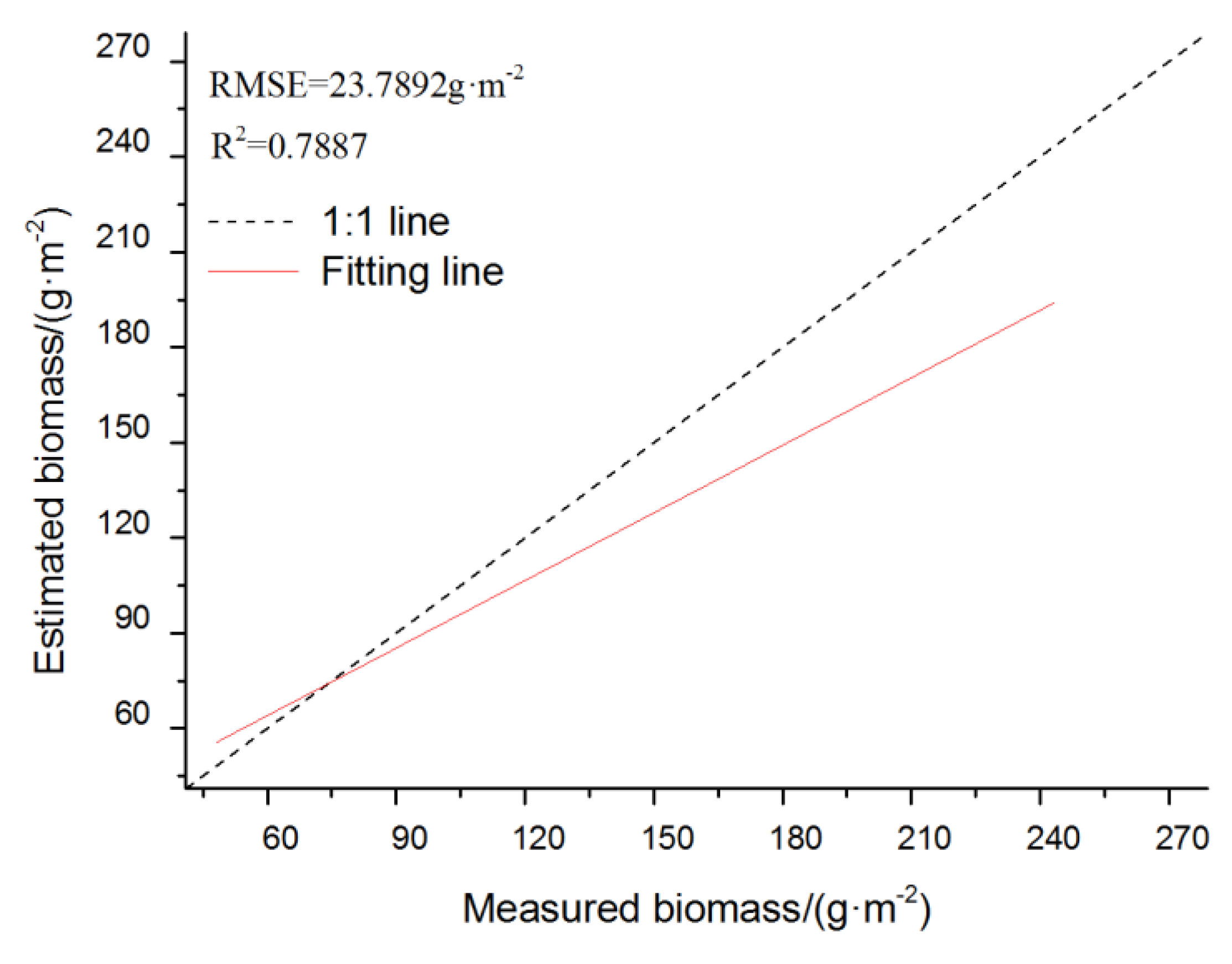
4.2. The Accuracy and Uncertainty of the AGB Estimation Model

When the WV-3 data is used alone, the regression model with an input variable of EVI shows moderate prediction performance with model accuracy of 73.12%. This model outperformed models based on SAR raw polarization backscatter coefficients. The estimation accuracy of the multispectral satellite-based biomass retrieval ranged from 67% to 85%. In grasslands, vegetation indices offer the advantage of superseding the influences of soil background, atmospheric composition, and the viewing and zenith angle effects, while enhancing the vegetation signal, when estimating AGB [41]. The regression model with an input variable of VH using Sentinel-1 SAR data only does not perform very well. The model accuracy is only at 0.43 for R² and 42.1104 g m⁻² for RMSE. Similar performance was found in the Sentinel-1 SAR value (R² = 0.34) reported by [42] for AGB estimation in grazing pastures involving two pasture sites. The active sensors are highly affected by topography due to incident angle, and by soil types [43]. The differential scattering of radar signal under different landforms in the rehabilitated dump might result in errors in the AGB estimation. Additionally, the influence of background, such as soil moisture and roughness in low-vegetation-coverage areas should be considered. In our studied rehabilitated area, the range of soil moisture was measured from 8% to 15% in the field survey and was relatively homogenous, which could contribute to low backscattering to AGB estimation [44]. However, soil particle size distribution is heterogeneous. Due to insufficient backfill soil after mining, the source of the topsoil is partly from coal ash, crushed rock, and quaternary sediments, which resulted in a higher coarse sand content and fine silt content [45]. Furthermore, the model accuracy should be linked to field sampling size and data extraction protocol utilized, a single Sentinel-1A pixel could have been extracted over each of the sample plots (the field plots were much smaller than the Sentinel-1A pixel). For a small-scale rehabilitated mining area using SAR data only, if the estimation results need to be more accurate, higher-resolution SAR images are required. Thus, given the relatively low relationship between shrub AGB and Sentienl-1A SAR data, it was suggested that the Sentienl-1A SAR parameter may provide additional biomass information as a supplement to the optical model [46]. The integration of optical and SAR technologies has also been proven to be more accurate than the individual technologies separately [47]. The model with fused-image band-8 input has the highest prediction accuracy (R² = 0.79, RMSE = 22.82 g m⁻²), which is more accurate in biomass prediction with less uncertainty in an area with a low vegetation cover. This can be ascribed to the ability of that model to accurately detect nonvegetated areas (which are smooth for radar waves) and with a low backscatter coefficient compared to the vegetated areas [48]. The Sentinel-1 C-band SAR is the preferred dataset for biomass analysis in low-biomass sites such as grasslands and forest regeneration sites. This is because of this data type has stronger backscattering in these areas compared to the L and P bands [49]. The critical problems of data saturation should be of concern, since these problems result in high uncertainties and low accuracies of AGB estimation in high-biomass areas [50]. For the C-band, the leaves and small branches remain as the major scattering components and the backscattering reaches saturation levels above 10 kg/m² in forest AGB estimation [51]. The highest uncertainty was found from an estimation model using SAR data only, and an uncertainty of 89.5 g m⁻² was recorded in the area with an AGB of 150–199.21 g m⁻². The data saturation problems could be partly solved by using multisource data or data fusion. Thus, the results indicated that the estimation model using fused-image bands and multiple variables both partly reduce the mean uncertainty value from the saturation level by a decrement of 2.42 g m⁻² to eventually become 9.68 g m⁻². The regression band based on the fused images developed in this work has the ability to estimate AGB values exceeding 100 g m⁻².

5. Conclusions

This paper indicates satisfactory results and suggests good potential for AGB mapping of rehabilitated vegetation area in mining sites. The availability of the WorldView-3 multispectral data of high spatial resolution and Sentinel-1 SAR data is an important development for small-scale mine rehabilitation and planning. The freely available SAR data should encourage the conduction of biomass mapping and monitoring with high accuracy in mining environments, particularly in semiarid grasslands. This work provides information which could be crucial for decision makers on mine rehabilitation planning and management of grassland systems. The following conclusions are drawn:

• High correlation values between biomass and remote-sensing data were obtained from the fused-image band 8 (0.874), EVI (0.876), VH polarization (0.504), and the mean texture parameter of band 7 (0.760) at a 0.01 significance level.
• The developed regression model based on the fused-image band 8 input provides a higher accuracy in biomass estimation compared to models using Worldview-3 or SAR data alone, which have prediction errors of 22.82 g m⁻² and 24.29 g m⁻², and accuracies of 74.64% and 73.12%, respectively.
• Higher values of uncertainty were found in the reclamation areas of 2013 and 2015 with an average AGB of over 100 g m⁻². The combination of the WV-3 and Sentinel-1 SAR data can reduce the uncertainty of the mean value from the saturation level by a decrement of 2.42 g m⁻² to eventually become 9.68 g m⁻².

References

1. Lv, X.; Xiao, W.; Zhao, Y.; Zhang, W.; Li, S.; Sun, H. Drivers of spatio-temporal ecological vulnerability in an arid, coal mining region in Western China. Ecol. Indic. 2019, 106, 105475. [Google Scholar] [CrossRef]
2. Erener, A. Remote sensing of vegetation health for reclaimed areas of Seyitömer open cast coal mine. Int. J. Coal Geol. 2011, 86, 20–26. [Google Scholar] [CrossRef]
3. Ahamed, T.; Tian, L.; Zhang, Y.; Ting, K.C. A review of remote sensing methods for biomass feedstock production. Biomass Bioenergy 2011, 35, 2455–2469. [Google Scholar] [CrossRef]
4. Townsend, P.A.; Helmers, D.P.; Kingdon, C.C.; McNeil, B.E.; de Beurs, K.M.; Eshleman, K.N. Changes in the extent of surface mining and reclamation in the Central Appalachians detected using a 1976–2006 Landsat time series. Remote. Sens. Environ. 2009, 113, 62–72. [Google Scholar] [CrossRef]
5. Bao, N.; Wu, L.; Ye, B.; Yang, K.; Zhou, W. Assessing soil organic matter of reclaimed soil from a large surface coal mine using a field spectroradiometer in laboratory. Geoderma 2017, 288, 47–55. [Google Scholar] [CrossRef]
6. Lu, D. The potential and challenge of remote sensing-based biomass estimation. Int. J. Remote Sens. 2006, 27, 1297–1328. [Google Scholar] [CrossRef]
7. Liu, C.-A.; Chen, Z.-X.; Shao, Y.; Chen, J.-S.; Hasi, T.; Pan, H.-Z. Research advances of SAR remote sensing for agriculture applications: A review. J. Integr. Agric. 2019, 18, 506–525. [Google Scholar] [CrossRef]
8. Hong, G.; Zhang, A.; Zhou, F.; Brisco, B. Integration of optical and synthetic aperture radar (SAR) images to differentiate grassland and alfalfa in Prairie area. Int. J. Appl. Earth Obs. Geoinf. 2014, 28, 12–19. [Google Scholar] [CrossRef]
9. McNairn, H.; Champagne, C.; Shang, J.; Holmstrom, D.; Reichert, G. Integration of optical and Synthetic Aperture Radar (SAR) imagery for delivering operational annual crop inventories. ISPRS J. Photogramm. Remote Sens. 2009, 64, 434–449. [Google Scholar] [CrossRef]
10. Zhao, P.; Lu, D.; Wang, G.; Liu, L.; Li, D.; Zhu, J.; Yu, S. Forest aboveground biomass estimation in Zhejiang Province using the integration of Landsat TM and ALOS PALSAR data. Int. J. Appl. Earth Obs. Geoinf. 2016, 53, 1–15. [Google Scholar] [CrossRef]
11. Maathuis, B.H.P.; van Genderen, J.L. A review of satellite and airborne sensors for remote sensing based detection of minefields and landmines. Int. J. Remote Sens. 2004, 25, 5201–5245. [Google Scholar] [CrossRef]
12. Blahwar, B.; Srivastav, S.K.; de Smeth, J.B. Use of high-resolution satellite imagery for investigating acid mine drainage from artisanal coal mining in North-Eastern India. Geocarto Int. 2012, 27, 231–247. [Google Scholar] [CrossRef]
13. Xian, G.; Shi, H.; Dewitz, J.; Wu, Z. Performances of WorldView 3, Sentinel 2, and Landsat 8 data in mapping impervious surface. Remote Sens. Appl. Soc. Environ. 2019, 15, 100246. [Google Scholar] [CrossRef]
14. Lukin, V.; Rubel, O.; Kozhemiakin, R. Despeckling of Multitemporal Sentinel SAR Images and Its Impact on Agricultural Area Classification; IntechOpen: London, UK, 2018. [Google Scholar]
15. Ma, W.; Pan, Z.; Guo, J.; Lei, B. Achieving Super-Resolution Remote Sensing Images via the Wavelet Transform Combined With the Recursive Res-Net. IEEE Trans. Geosci. Remote Sens. 2019, 57, 1–16. [Google Scholar] [CrossRef]
16. Luo, Z.; Wu, J. A POCS Super-Resolution Image Reconstruction based on the Projection Residue. Proc. SPIE Int. Soc. Opt. Eng. 2011, 8349, 14. [Google Scholar]
17. Gan, X.; Liew, A.W.-C.; Yan, H. A POCS-based constrained total least squares algorithm for image restoration. J. Vis. Commun. Image Represent. 2006, 17, 986–1003. [Google Scholar] [CrossRef]
18. Otukei, J.R.; Blaschke, T.; Collins, M. Fusion of TerraSAR-x and Landsat ETM+ data for protected area mapping in Uganda. Int. J. Appl. Earth Obs. Geoinf. 2015, 38, 99–104. [Google Scholar] [CrossRef]
19. Fu, B.; Wang, Y.; Campbell, A.; Li, Y.; Zhang, B.; Yin, S.; Xing, Z.; Jin, X. Comparison of object-based and pixel-based Random Forest algorithm for wetland vegetation mapping using high spatial resolution GF-1 and SAR data. Ecol. Indic. 2017, 73, 105–117. [Google Scholar] [CrossRef]
20. Rouse, J.W.; Hass, R.H.; Schell, J.A.; Deering, D.W. Monitoring vegetation systems in the great plains with ERTS. In Proceedings of the Third Earth Resources Technology Satellite-1 Symposium, Washington, DC, USA, 10–14 December 1973. [Google Scholar]
21. Richardson, A.J.; Wiegand, C.L. Distinguishing vegetation from soil background information. Eng. Remote Sens. 1977, 43, 1541–1552. [Google Scholar]
22. Pearson, R.L.; Miller, L.D. Remote Mapping of Standing Crop Biomass for Estimation of the Productivity of the Short-Grass Prairie. In Proceedings of the 8th International Symposium on Remote Sensing of Environment, Ann Arbor, MI, USA, 2–6 October 1972. [Google Scholar]
23. Gitelson, A.A.; Kaufman, Y.J.; Merzlyak, M.N. Use of a green channel in remote sensing of global vegetation from EOS-MODIS. Remote Sens. Environ. 1996, 58, 289–298. [Google Scholar] [CrossRef]
24. Kaufman, Y.J.; Tanre, D. Atmospherically resistant vegetation index (ARVI) for EOS-MODIS. IEEE Trans. Geosci. Remote Sens. 1992, 30, 261–270. [Google Scholar] [CrossRef]
25. Liu, H.Q.; Huete, A. A feedback based modification of the NDVI to minimize canopy background and atmospheric noise. IEEE Trans. Geosci. Remote Sens. 1995, 33, 457–465. [Google Scholar] [CrossRef]
26. Sims, D.A.; Gamon, J.A. Relationships between leaf pigment content and spectral reflectance across a wide range of species, leaf structures and developmental stages. Remote Sens Environ. 2002, 81, 337–354. [Google Scholar] [CrossRef]
27. Wang, D.; Wan, B.; Qiu, P.; Su, Y.; Wu, X. Evaluating the Performance of Sentinel-2, Landsat 8 and Pléiades-1 in Mapping Mangrove Extent and Species. Remote Sens. 2018, 10, 1468. [Google Scholar] [CrossRef]
28. Sidike, P.; Sagan, V.; Maimaitijiang, M.; Maimaitiyiming, M.; Shakoor, N.; Burken, J.; Mockler, T.; Fritschi, F.B. dPEN: Deep Progressively Expanded Network for mapping heterogeneous agricultural landscape using WorldView-3 satellite imagery. Remote Sens. Environ. 2019, 221, 756–772. [Google Scholar] [CrossRef]
29. Marshall, V.; Lewis, M.; Ostendorf, B. Do additional bands (Coastal, NIR-2, Red-Edge and Yellow) in worldview-2 multispectral imagery improve discrimination of an invasive Tussock, Buffel Grass (Cenchrus Ciliaris)? In Proceedings of the International Archives of the Photogrammetry, Remote Sensing and Spatial Information Science, Melbourne, Australia, 25 August–1 September 2012. [Google Scholar]
30. Liu, L.; Wang, J.; Huang, W.; Zhao, C.; Zhang, B.; Tong, Q. Estimating winter wheat plant water content using red edge parameters. Int. J. Remote Sens. 2004, 25, 3331–3342. [Google Scholar] [CrossRef]
31. Dong, T.; Liu, J.; Shang, J.; Qian, B.; Ma, B.; Kovacs, J.M.; Walters, D.; Jiao, X.; Geng, X.; Shi, Y. Assessment of red-edge vegetation indices for crop leaf area index estimation. Remote Sens. Environ. 2019, 222, 133–143. [Google Scholar] [CrossRef]
32. Maimaitijiang, M.; Ghulam, A.; Sidike, P.; Hartling, S.; Maimaitiyiming, M.; Peterson, K.; Shavers, E.; Fishman, J.; Peterson, J.; Kadam, S.; et al. Unmanned Aerial System (UAS)-based phenotyping of soybean using multi-sensor data fusion and extreme learning machine. ISPRS J. Photogramm. Remote Sens. 2017, 134, 43–58. [Google Scholar] [CrossRef]
33. Schultz, M.; Clevers, J.G.P.W.; Carter, S.; Verbesselt, J.; Avitabile, V.; Quang, H.V.; Herold, M. Performance of vegetation indices from Landsat time series in deforestation monitoring. Int. J. Appl. Earth Obs. Geoinf. 2016, 52, 318–327. [Google Scholar] [CrossRef]
34. Kumar, V.; Sharma, A.; Bhardwaj, R.; Thukral, A.K. Comparison of different reflectance indices for vegetation analysis using Landsat-TM data. Remote Sens. Appl. Soc. Environ. 2018, 12, 70–77. [Google Scholar] [CrossRef]
35. Barati, S.; Rayegani, B.; Saati, M.; Sharifi, A.; Nasri, M. Comparison the accuracies of different spectral indices for estimation of vegetation cover fraction in sparse vegetated areas. Egypt. J. Remote Sens. Space Sci. 2011, 14, 49–56. [Google Scholar] [CrossRef]
36. Wood, E.M.; Pidgeon, A.M.; Radeloff, V.C.; Keuler, N.S. Image texture as a remotely sensed measure of vegetation structure. Remote Sens. Environ. 2012, 121, 516–526. [Google Scholar] [CrossRef]
37. Hlatshwayo, S.T.; Mutanga, O.; Lottering, R.T.; Kiala, Z.; Ismail, R. Mapping forest aboveground biomass in the reforested Buffelsdraai landfill site using texture combinations computed from SPOT-6 pan-sharpened imagery. Int. J. Appl. Earth Obs. Geoinf. 2019, 74, 65–77. [Google Scholar] [CrossRef]
38. Fan, W.; Chao, W.; Hong, Z.; Bo, Z.; Tang, Y. Rice crop monitoring in South China with RADARSAT-2 quad-polarization SAR data. IEEE Geosci. Remote Sens. Lett. 2011, 8, 196–200. [Google Scholar]
39. Liu, Y.; Gong, W.; Xing, Y.; Hu, X.; Gong, J. Estimation of the forest stand mean height and aboveground biomass in Northeast China using SAR Sentinel-1B, multispectral Sentinel-2A, and DEM imagery. ISPRS J. Photogramm. Remote Sens. 2019, 151, 277–289. [Google Scholar] [CrossRef]
40. Bigdeli, B.; Pahlavani, P. High resolution multisensor fusion of SAR, optical and LiDAR data based on crisp vs. fuzzy and feature vs. decision ensemble systems. Int. J. Appl. Earth Obs. Geoinf. 2016, 52, 126–136. [Google Scholar] [CrossRef]
41. Naidoo, L.; van Deventer, H.; Ramoelo, A.; Mathieu, R.; Nondlazi, B.; Gangat, R. Estimating above ground biomass as an indicator of carbon storage in vegetated wetlands of the grassland biome of South Africa. Int. J. Appl. Earth Obs. Geoinf. 2019, 78, 118–129. [Google Scholar] [CrossRef]
42. Wang, J.; Xiao, X.; Bajgain, R.; Starks, P.; Steiner, J.; Doughty, R.B.; Chang, Q. Estimating leaf area index and aboveground biomass of grazing pastures using Sentinel-1, Sentinel-2 and Landsat images. ISPRS J. Photogramm. Remote Sens. 2019, 154, 189–201. [Google Scholar] [CrossRef] [Green Version]
43. GhasemiMahmod, N.; Saheb, R.S.R.; Mohammadzadeh, A.M. A review on biomass estimation methods using synthetic aperture radar data. Int. J. Ofgeomatics Geosci. 2011, 1, 776–782. [Google Scholar]
44. Millard, K.; Richardson, M. Quantifying the relative contributions of vegetation and soil moisture conditions to polarimetric C-Band SAR response in a temperate peatland. Remote Sens. Environ. 2018, 206, 123–138. [Google Scholar] [CrossRef]
45. Bao, N.; Liu, S.; Zhou, Y. Predicting particle-size distribution using thermal infrared spectroscopy from reclaimed mine land in the semi-arid grassland of North China. CATENA 2019, 183, 104190. [Google Scholar] [CrossRef]
46. Chang, J.; Shoshany, M. Mediterranean shrublands biomass estimation using Sentinel-1 and Sentinel-2. In Proceedings of the 2016 IEEE International Geoscience and Remote Sensing Symposium (IGARSS), Beijing, China, 10–15 July 2016; pp. 5300–5303. [Google Scholar]
47. Chudong, H.; Xinyue, Y.; Chengbin, D.; Zili, Z.; Zi, W. Mapping Above-Ground Biomass by Integrating Optical and SAR Imagery: A Case Study of Xixi National Wetland Park, China. Remote Sens. 2016, 8, 647. [Google Scholar]
48. Kumar, S.; Pandey, U.; Kushwaha, S.P.; Chatterjee, R.S.; Bijker, W. Aboveground biomass estimation of tropical forest from Envisat advanced synthetic aperture radar data using modeling approach. J. Appl. Remote Sens. 2012, 6, 063588. [Google Scholar] [CrossRef]
49. Sinha, S.; Jeganathan, C.; Sharma, L.K.; Nathawat, M.S. A review of radar remote sensing for biomass estimation. Int. J. Environ. Sci. Technol. 2015, 12, 1779–1792. [Google Scholar] [CrossRef] [Green Version]
50. Vafaei, S.; Soosani, J.; Adeli, K.; Fadaei, H.; Naghavi, H.; Pham, T.; Tien Bui, D. Improving Accuracy Estimation of Forest Aboveground Biomass Based on Incorporation of ALOS-2 PALSAR-2 and Sentinel-2A Imagery and Machine Learning: A Case Study of the Hyrcanian Forest Area (Iran). Remote Sens. 2018, 10, 172. [Google Scholar] [CrossRef] [Green Version]
51. Ranson, K.J.; Sun, G. Mapping biomass of a northern forest using multifrequency SAR data. Geosci. Remote Sens. IEEE Trans. 1994, 32, 388–396. [Google Scholar] [CrossRef]
Figure 1. Location of the research area (left). Photograph of the mine area showing sampling sites in rehabilitated dump (middle). Digital elevation model (DEM) of the studied dump (right).
Remotesensing 11 02855 g001
Figure 2. Preprocessing procedures for synthetic aperture radar (SAR) images.
Remotesensing 11 02855 g002
Figure 3. SAR vertical and vertical polarization (VV) image visualization before and after image reconstruction.
Remotesensing 11 02855 g003
Figure 4. SAR vertical and horizon polarization (VH) image visualization before and after image reconstruction.
Remotesensing 11 02855 g004
Figure 5. The fused image integrating the Sentinel-SAR image with the WV-3 image.
Remotesensing 11 02855 g005
Figure 6. The entropy value for all spectral bands of WV-3, VV polarization of the SAR image, and fused bands.
Remotesensing 11 02855 g006
Figure 7. The average gradient value for all available bands of WV-3, VV polarization of the SAR image, and fused bands.
Remotesensing 11 02855 g007
Figure 8. The similarity coefficient and the spectral distortion between the WV-3 image and the fused image for all spectral bands.
Remotesensing 11 02855 g008
Figure 9. The relationship between measured and retrieved above-ground biomass (AGB) from the best biomass prediction models of Table 6.
Remotesensing 11 02855 g009
Figure 10. The relationship between measured AGB of 2018 and 2019 and retrieved AGB from the biomass prediction model based on the fusion band.
Remotesensing 11 02855 g010
Figure 11. Residual distributions of the best biomass prediction models of Table 6.
Remotesensing 11 02855 g011
Figure 12. Biomass mapping for the best four biomass prediction models of Table 6.
Remotesensing 11 02855 g012aRemotesensing 11 02855 g012b
Figure 13. Biomass uncertainty for the best four biomass prediction models of Table 6
Remotesensing 11 02855 g013aRemotesensing 11 02855 g013b