Modified Search Strategies Assisted Crossover Whale Optimization Algorithm with Selection Operator for Parameter Extraction of Solar Photovoltaic Models

Abstract

Extracting accurate values for involved unknown parameters of solar photovoltaic (PV) models is very important for modeling PV systems. In recent years, the use of metaheuristic algorithms for this problem tends to be more popular and vibrant due to their efficacy in solving highly nonlinear multimodal optimization problems. The whale optimization algorithm (WOA) is a relatively new and competitive metaheuristic algorithm. In this paper, an improved variant of WOA referred to as MCSWOA, is proposed to the parameter extraction of PV models. In MCSWOA, three improved components are integrated together: (i) Two modified search strategies named WOA/rand/1 and WOA/current-to-best/1 inspired by differential evolution are designed to balance the exploration and exploitation; (ii) a crossover operator based on the above modified search strategies is introduced to meet the search-oriented requirements of different dimensions; and (iii) a selection operator instead of the “generate-and-go” operator used in the original WOA is employed to prevent the population quality getting worse and thus to guarantee the consistency of evolutionary direction. The proposed MCSWOA is applied to five PV types. Both single diode and double diode models are used to model these five PV types. The good performance of MCSWOA is verified by various algorithms.

1. Introduction

Solar energy is an inexhaustible and carbon emission-free energy source to promote sustainable development. Solar photovoltaic (PV) is becoming the preferred choice for meeting the rapidly growing power demands globally [1,2]. It is a clean energy according to the principle of sustainability. Take China as an example, according to the latest data from the National Energy Administration, PV added 5.20GW capacity, which was more than that of wind (added 4.78GW) in the first quarter of 2019 [3]. In addition, by the end of the first quarter of 2019, the total installed PV capacity had reached 180GW, accounting for 24.3% of renewable energy, only 0.09GW below that of wind, and the gap is narrowing. Along with the increasing installed capacity of PV, its impact on the connected power system is growing, and thereby, analyzing PV systems’ dynamic conversion behavior is quite important and necessary. Thereinto, accurate modeling of the PV system’s basic device, i.e., the PV cell or module, is the premise and crux. The most widely used modeling tool is the single diode (SDM) and double diode (DDM) equivalent circuit models [4]. The SDM and DDM have five and seven unknown model parameters, respectively, and extracting accurate values for these parameters is just the purpose of this study.

Many methods have been proposed to solve the parameter extraction problem of PV models. They can be categorized into analytical methods and optimization methods approximately. Analytical methods mainly use some special data points such as short-circuit point, open-circuit point, and maximum power point of the current-voltage (I–V) characteristic curve under standard test conditions (STC) to formulate a few mathematical equations for the unknown model parameters. They have the features of simplicity, rapidity, and convenience. Their extraction accuracy is directly subject to the selected special data points provided by the manufacturers. In this context, the incorrectly specified values for these data points will degrade the extraction accuracy considerably due to the extraction strategy of “taking a part for the whole” [5,6]. In addition, those employed special data points are factory measured under the STC, while the PV degradation makes the model parameters change over time [7], which further influences the extraction accuracy of the “taking a part for the whole” methods.

Different from the analytical methods, the optimization methods abandon the heavy dependence on several special data points and use a number of actual measured data points to extract the unknown model parameters. First, an optimization objective function is constructed to reflect the difference between the measured data and the calculated data based on the idea of curve fitting. Then, solution optimization methods, including deterministic methods and metaheuristic methods, are designed to minimize the objective function and thereby to obtain the values for the unknown model parameters. These solution methods can overcome the shortcomings of the analytical methods thanks to “taking all actual measured data” rather than “taking a part of factory measured data” for the whole. The deterministic methods such as the Newton method, Newton–Raphson method and Levenberg–Marquardt algorithm are gradient-based methods. They are likely to get stuck in local optima especially for complicated multimodal problems such as the one considered in this work. Additionally, simplification and linearization are frequently performed to ease the optimization procedure. Consequently, they may result in poor approximate and unreliable solutions [8].

Metaheuristic methods, alternatively, do not use the gradient information and make no simplification or linearization to the optimization procedure. Therefore, they can hedge the problems of deterministic methods and have attracted growing attention recently. Many metaheuristic methods concluding particle swarm optimization (PSO) [9,10,11], differential evolution (DE) [12], teaching-learning-based optimization (TLBO) [13,14], supply-demand-based optimization (SDO) [15], symbiotic organisms search algorithm (SOS) [16], JAYA algorithm [17], artificial bee colony (ABC) [18], imperialist competitive algorithm [19], flower pollination algorithm (FPA) [20], hybrid algorithms [21,22,23,24], etc., have been applied to the parameter extraction problem of PV models.

The whale optimization algorithm (WOA) [25] is a new and versatile metaheuristic method inspired by the special spiral bubble-net hunting behavior of humpback whales. It performs effectively, competitively, and has been applied to various engineering optimization problems, including the parameter extraction problem of PV models. For example, Oliva et al. [26] utilized the chaotic maps to improve the performance of WOA and then applied the modified WOA to the concerned problem here. Abd Elaziz and Oliva [27] employed the opposition-based learning to enhance the exploration of WOA and applied the resultant WOA variant to both benchmark optimization functions and the problem considered here. Xiong et al. [28] developed two improved search strategies to balance WOA’s local exploitation and global exploration, and then applied the improved WOA to different PV models. In reference [29], Xiong et al. used DE to enhance the exploration of WOA and then employed the hybrid algorithm to both benchmark optimization functions and different PV models.

From our previous works [28,29], we know that the original WOA performs well in local exploitation but badly in global exploration, which easily leads to premature convergence. They also reveal that the use of both improved search strategies and DE can enhance the performance of WOA significantly. Having noticed this, in this paper, we propose two modified search strategies named WOA/rand/1 and WOA/current-to-best/1 inspired by DE. The former uses one random weighted difference vector to perturb a randomly selected individual and thus to improve the exploration; while the latter simultaneously adopts one current-to-best weighted difference vector and one random weighted difference vector to perturb the current individual and thereby to maintain the exploitation. In addition, in the original WOA, the values of all dimensions of each offspring completely come from a vector generated by one search strategy, which cannot meet the exploration and exploitation performance requirements of different dimensions. In this case, a crossover operator based on the modified search strategies is designed. It adopts two different search strategies to generate each offspring simultaneously, which can further promote the balance between exploration and exploitation. Moreover, the original WOA preserves the generated vector regardless of its quality. This “generate-and-go” strategy may result in retrogression or oscillation in evolutionary process. To prevent this phenomenon from occurring, a selection operator instead of the “generate-and-go” operator is implemented to guarantee the consistency of evolutionary direction. The resultant improved variant of WOA, referred to as MCSWOA, is applied to five PV types modeled by both SDM and DDM.

The main contributions of this paper are the following:

(1)

An improved variant of WOA, i.e., MCSWOA, is presented to parameter extraction of PV models. In MCSWOA, three improved components, including two modified search strategies, a crossover operator, and a selection operator are developed and integrated well to enhance its performance.

(2)

MCSWOA is applied to five PV types, including RTC France cell, Photowatt-PWP201 module, STM6-40/36 module, STP6-120/36 module, and Sharp ND-R250A5 module. Both SDM and DDM are used to model these five PV types.

(3)

The good performance of MCSWOA in extracting accurate parameters of PV models is fully verified through comparison with other 31 algorithms in terms of the parameter accuracy, convergence speed, robustness, and statistics.

The rest of this paper is organized as follows. In Section 2, the mathematical formulation of the parameter extraction problem is described. Section 3 introduces the original WOA. Section 4 gives the proposed MCSWOA. Section 5 presents the experimental results and comparisons. The discussions are provided in Section 6. Finally, the paper is concluded in Section 7.

2. Problem Formulation

2.1. Single Diode Model (SDM)

The equivalent circuit of SDM is presented in Figure 1.

The output current $I_{\mathrm{L}}$ can be achieved according to the Kirchhoff’s current law:

$$I_{\mathrm{L}}=I_{\mathrm{ph}}-I_{\mathrm{d}}-I_{\mathrm{sh}}$$

(1)

where $I_{\mathrm{ph}}$, $I_{\mathrm{sh}}$ and $I_{\mathrm{d}}$ are the photogenerated current, shunt resistor current, and diode current, respectively. $I_{\mathrm{d}}$ and $I_{\mathrm{sh}}$ are calculated as follows [4,6]:

$$I_{\mathrm{d}}=I_{\mathrm{sd}}·[\exp (\frac{V_{\mathrm{L}}+R_{\mathrm{s}}·I_{\mathrm{L}}}{n{V}_{\mathrm{t}}})-1]$$

(2)

$$V_{\mathrm{t}}=\frac{kT}{q}$$

(3)

$$I_{\mathrm{sh}}=\frac{V_{\mathrm{L}}+R_{\mathrm{s}}·I_{\mathrm{L}}}{R_{\mathrm{sh}}}$$

(4)

where $I_{\mathrm{sd}}$ is the saturation current, $V_{\mathrm{L}}$ is the output voltage, $R_{\mathrm{s}}$ and $R_{\mathrm{sh}}$ are the series and shunt resistances, respectively, $n$ is the diode ideal factor, $k$ is the Boltzmann constant (1.3806503 × 10⁻²³ J/K), $q$ is the electron charge (1.60217646 × 10⁻¹⁹ C), and $T$ is the cell temperature (K).

The output current $I_{\mathrm{L}}$ can be obtained by substituting Equations (2) and (4) into (1):

$$I_{\mathrm{L}}=I_{\mathrm{ph}}-I_{\mathrm{sd}}·[\exp (\frac{V_{\mathrm{L}}+R_{\mathrm{s}}·I_{\mathrm{L}}}{n{V}_{\mathrm{t}}})-1]-\frac{V_{\mathrm{L}}+R_{\mathrm{s}}·I_{\mathrm{L}}}{R_{\mathrm{sh}}}$$

(5)

From Equation (5), it can be seen that the SDM has 5 unknown parameters (i.e., $I_{\mathrm{ph}},I_{\mathrm{sd}},R_{\mathrm{s}},R_{\mathrm{sh}},\mathrm{and}n$) that need to be extracted.

2.2. Double Diode Model (DDM)

When considering the effect of the recombination current loss in the depletion region, we can get the equivalent circuit of DDM, as shown in Figure 2. It performs well in some applications [4].

The output current $I_{\mathrm{L}}$ is calculated as follows:

$$\begin{array}{l}{I}_{\mathrm{L}}=I_{\mathrm{ph}}-I_{\mathrm{d}1}-I_{\mathrm{d}2}-I_{\mathrm{sh}}\\ =I_{\mathrm{ph}}-I_{\mathrm{sd}1}·[\exp (\frac{V_{\mathrm{L}}+R_{\mathrm{s}}·I_{\mathrm{L}}}{n_1{V}_{\mathrm{t}}})-1]\\ -I_{\mathrm{sd}2}·[\exp (\frac{V_{\mathrm{L}}+R_{\mathrm{s}}·I_{\mathrm{L}}}{n_2{V}_{\mathrm{t}}})-1]-\frac{V_{\mathrm{L}}+R_{\mathrm{s}}·I_{\mathrm{L}}}{R_{\mathrm{sh}}}\end{array}$$

(6)

where $I_{\mathrm{sd}1}$ and $I_{\mathrm{sd}2}$ are diode currents, $n_1$ and $n_2$ are diode ideal factors. The DDM has 7 unknown parameters (i.e., $I_{\mathrm{ph}},I_{\mathrm{sd}1},I_{\mathrm{sd}2},R_{\mathrm{s}},R_{\mathrm{sh}},n_1\mathrm{and}{n}_2$) that need to be extracted.

2.3. PV Module Model

For a PV module with $N_{\mathrm{s}}\times N_{\mathrm{p}}$ solar cells in series and/or in parallel, its output current $I_{\mathrm{L}}$ can be formulated as follows:

For the SDM based PV module:

$$I_{\mathrm{L}}=N_{\mathrm{p}}\left\{I_{\mathrm{ph}}-I_{\mathrm{sd}}·[\exp (\frac{V_{\mathrm{L}}/N_{\mathrm{s}}+R_{\mathrm{s}}{I}_{\mathrm{L}}/N_{\mathrm{p}}}{n{V}_{\mathrm{t}}})-1]-\frac{V_{\mathrm{L}}/N_{\mathrm{s}}+R_{\mathrm{s}}{I}_{\mathrm{L}}/N_{\mathrm{p}}}{R_{\mathrm{sh}}}\right\}$$

(7)

For the DDM based PV module:

$$I_{\mathrm{L}}=N_{\mathrm{p}}\left\{\begin{array}{l}{I}_{\mathrm{ph}}-I_{\mathrm{sd}1}·[\exp (\frac{V_{\mathrm{L}}/N_{\mathrm{s}}+R_{\mathrm{s}}{I}_{\mathrm{L}}/N_{\mathrm{p}}}{n_1{V}_{\mathrm{t}}})-1]\\ -I_{\mathrm{sd}2}·[\exp (\frac{V_{\mathrm{L}}/N_{\mathrm{s}}+R_{\mathrm{s}}{I}_{\mathrm{L}}/N_{\mathrm{p}}}{n_2{V}_{\mathrm{t}}})-1]-\frac{V_{\mathrm{L}}/N_{\mathrm{s}}+R_{\mathrm{s}}{I}_{\mathrm{L}}/N_{\mathrm{p}}}{R_{\mathrm{sh}}}\end{array}\right\}$$

(8)

2.4. Objective Function

One way to extract the unknown parameters of PV models is to construct an objective function to reflect the difference between the measured data and the calculated data. Commonly, the root mean square error (RMSE) between the measured current $I_{L,\mathrm{measured}}$ and the calculated current $I_{L,\mathrm{calculated}}$ as shown in Equation (9) is recommended [6,8,9,30,31].

$$\min f(x)=\mathrm{RMSE}(x)=\sqrt{\frac{1}{N}{\displaystyle {\sum }_{k=1}^N{[I_{L,\mathrm{calculated}}^k(x)-I_{L,\mathrm{measured}}^k]}^2}}$$

(9)

where $N$ is the number of measured data, $x$ is the vector of unknown parameters.

3. Whale Optimization Algorithm

WOA [25] is an effective metaheuristic inspired by the special spiral bubble-net hunting behavior of humpback whales. In WOA, the position of each whale (i.e., population individual) is represented as $x_i^t=[x_{i,1}^t,x_{i,2}^t,\dots ,x_{i,D}^t]$, where $i=1,2,\dots ,ps$, $t=1,2,\dots ,t_{\max }$, $ps$ is the population size, $t_{\max }$ is the maximum number of iterations, and $D$ is the dimension of one individual. WOA contains the following three parts:

(1) Encircling prey

WOA defines the position of a current best humpback whale as the target prey, and other whales encircle the prey using the following formulation:

$$x_i^{t+1}=x_g^t-A·|C·x_g^t-x_i^t|$$

(10)

where $x_g^t$ is the best position found so far. $A$ and $C$ are coefficient parameters and calculated for each individual using the following method:

$$A=2·a·r-a$$

(11)

$$C=2·r$$

(12)

where $a$ linearly decreases from 2 to 0 with the increasing of iterations. $r$ is a random real number in (0,1).

(2) Bubble-net attacking method

WOA employs both shrinking encircling and spiraling to spin around the prey with the same probability as follows:

$$x_i^{t+1}=x_g^t-A·|C·x_g^t-x_i^t|\mathrm{if}p<0.5$$

(13)

$$x_i^{t+1}=x_g^t+\exp (bl)·\cos (2\pi l)·|x_g^t-x_i^t|\mathrm{if}p\ge 0.5$$

(14)

where $b$ is a constant for defining the shape of the logarithmic spiral, $l$ and $p$ are random real numbers in (0,1).

(3) Searching for prey

Before finding the prey, humpback whales swim around and select a random whale to search for prey. This behavior is formulated as follows and continues if $|A|\ge 1$.

$$x_i^{t+1}=x_r^t-A·|C·x_r^t-x_i^t|$$

(15)

where $r\in \{1,2,\dots ,ps\}$ is different from $i$.

4. The Proposed MCSWOA

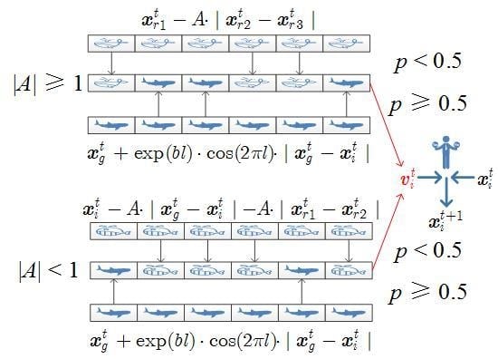
4.1. Modified Search Strategies

It is well-known that balancing exploration and exploitation is very important for a metaheuristic algorithm. For the original WOA, it emphasizes the exploitation excessively and thus easily suffers from premature convergence [28]. In order to solve this issue, one active method is to modify its search strategy.

Differential evolution (DE) [32] has proved its efficiency in solving different real-world problems. The efficiency of DE comes largely from its versatile mutation strategies. The following are 2 popular mutation strategies widely used in the literature:

$$\mathrm{DE}/\mathrm{rand}/1:v_i^t=x_{r1}^t+F·(x_{r2}^t-x_{r3}^t)$$

(16)

$$\mathrm{DE}/\mathrm{current}-\mathrm{to}-\mathrm{best}/1:v_i^t=x_i^t+F·(x_g^t-x_i^t)+F·(x_{r1}^t-x_{r2}^t)$$

(17)

where $r1$, $r2$ and $r3$ are random distinct integers selected from $\{1,2,\cdots ,ps\}$ and are also different from $i$, the parameter $F$ is the scaling factor. The former, i.e., DE/rand/1 strategy, usually presents good exploration while the latter, i.e., DE/current-to-best/1 strategy exhibits good exploitation.

Inspired by the mutation strategies of DE, in this paper, two modified search strategies are proposed to generate new donor individuals as follows:

$$\mathrm{WOA}/\mathrm{rand}/1:v_i^t=x_{r1}^t-A·|x_{r2}^t-x_{r3}^t|$$

(18)

$$\mathrm{WOA}/\mathrm{current}-\mathrm{to}-\mathrm{best}/1:v_i^t=x_i^t-A·|x_g^t-x_i^t|-A·|x_{r1}^t-x_{r2}^t|$$

(19)

The above-modified search strategies are employed to replace Equations (15) and (13), respectively.

4.2. Modified Search Strategies Assisted Crossover Operator

In the original WOA, the random parameter $p$ is generated for each individual, indicating that all dimensions would perform the same search strategy. For example, on the premise of $|A|\ge 1$, if $p<0.5$, then the current individual would perform Equation (15). According to Equation (15), WOA updates the current individual around a random individual $x_r^t$, which is beneficial for the exploration but harmful to the exploitation. In fact, different dimensions of an individual have different performance requirements for exploration and exploitation. For one dimension, it is wise to perform the exploration-oriented search strategy if the population diversity associated with this dimension is high; otherwise, it is wise to perform the exploitation-oriented search strategy. In order to meet the performance requirements of different dimensions, a crossover operator based on the abovementioned modified search strategies is proposed and shown in Figure 3. In the crossover operator, for each dimension of each individual, the random parameter $p$ is regenerated, and thereby the target dimension of the donor individual has the same chance of deriving from 2 search strategies, which is able to promote the balance between the exploration and exploitation. This crossover operator can be formulated as follows:

$$v_{i,d}^t=\{\begin{array}{l}\{\begin{array}{l}{x}_{r1,d}^t-A·|x_{r2,d}^t-x_{r3,d}^t|\mathrm{if}p<0.5\\ x_{g,d}^t+\exp (bl)·\cos (2\pi l)·|x_{g,d}^t-x_{i,d}^t|\mathrm{if}p\ge 0.5\end{array}\mathrm{if}|A|\ge 1\\ \{\begin{array}{l}{x}_{i,d}^t-A·|x_{g,d}^t-x_{i,d}^t|-A·|x_{r1,d}^t-x_{r2,d}^t|\mathrm{if}p<0.5\\ x_{g,d}^t+\exp (bl)·\cos (2\pi l)·|x_{g,d}^t-x_{i,d}^t|\mathrm{if}p\ge 0.5\end{array}\mathrm{if}|A|<1\end{array}$$

(20)

4.3. Selection Operator

In the original WOA, the target individual is directly replaced by the newly generated vector regardless of its quality. This “generate-and-go” operator is not very effective because the newly generated vector may be worse than the target individual. In order to guarantee the consistency of evolutionary direction, a selection operator is employed to determine whether the target individual or the donor individual survives to the next iteration. This selection operator is formulated as follows:

$$x_i^{t+1}=\{\begin{array}{l}{v}_i^t\mathrm{if}f(v_i^t)\le f(x_i^t)\\ x_i^t\mathrm{if}f(v_i^t)>f(x_i^t)\end{array}$$

(21)

Hence, the prerequisite of using the donor individual to replace the target individual is that the donor individual achieves an equal or better fitness value; otherwise, the donor individual is abandoned, and the target individual is retained and passed on to the next iteration. Consequently, the population either gains quality improvement or maintains the current quality level, but never gets worse.

4.4. The Main Procedure of MCSWOA

By combining the abovementioned 3 improved components into WOA, the MCSWOA is developed and presented in Algorithm 1. Compared with the original WOA, it can be seen that: (1) MCSWOA needs only a small extra computational cost in comparing the fitness values of current individuals with those of donor individuals. (2) The structure of MCSWOA also remains very simple, and no new parameter that needed to be adjusted is introduced. (3) The use of the selection operator makes MCSWOA an elitist method that is able to preserve best individuals in the population.

Algorithm 1: The main procedure of MCSWOA
1:	Generate a random initial population
2:	Evaluate the fitness for each individual
3:	Select the best individual $x_{\mathrm{best}}^0$ and set it as $x_g^0$
4:	Initialize the iteration counter $t=1$
5:	While the stopping condition is not satisfied do
6:	for $i=1$ to $ps$ do
7:	Update $a$, $A$, and $l$
8:	for $d=1$ to $D$ do
9:	Update $p$
10:	if $p<0.5$ then
11:	Select three random individuals $x_{r1}^t\ne x_{r2}^t\ne x_{r3}^t\ne x_i^t$
12:	if $|A|\ge 1$ then
13:	$v_{i,d}^t=x_{r1,d}^t-A·|x_{r2,d}^t-x_{r3,d}^t|$
14:	else
15:	$v_{i,d}^t=x_{i,d}^t-A·|x_{g,d}^t-x_{i,d}^t|-A·|x_{r1,d}^t-x_{r2,d}^t|$
16:	end if
17:	else
18:	$v_{i,d}^{t+1}=x_{g,d}^t+\exp (bl)·\cos (2\pi l)·|x_{g,d}^t-x_{i,d}^t|$
19:	end if
20:	end for
21:	end for
22:	Evaluate the fitness for each donor individual
23:	for $i=1$ to $ps$ do
24:	if $f(v_i^t)\le f(x_i^t)$ then
25:	$x_i^{t+1}=v_i^t$
26:	else
27:	$x_i^{t+1}=x_i^t$
28:	end if
29:	end for
30:	Select the best individual $x_{\mathrm{best}}^t$ of the updated population
31:	if $f(x_{\mathrm{best}}^t)\le f(x_g^t)$ then
32:	$x_g^{t+1}=x_{\mathrm{best}}^t$
33:	else
34:	$x_g^{t+1}=x_g^t$
35:	end if
36:	$t=t+1$
37:	End while

5. Experimental Results

5.1. Test Cases

In this work, the proposed MCSWOA was applied to five PV types, including RTC France cell, Photowatt-PWP201 module, STM6-40/36 module, STP6-120/36 module, and Sharp ND-R250A5 module. Both the SDM and DDM were adopted to model them, and thus we could get 10 test cases. The detailed information about these 10 test cases is tabulated in

Table 1. Test photovoltaic (PV) models in this work.

Case	PV Type	Number of Cells (Ns × Np)	Irradiance (W/m2)	Temperature (°C)	PV model
1/2	RTC France cell	1 × 1	1000	33	SDM/DDM
3/4	Photowatt-PWP201 module	36 × 1	1000	45	SDM/DDM
5/6	STM6-40/36 module	36 × 1	NA	51	SDM/DDM
7/8	STP6-120/36 module	36 × 1	NA	55	SDM/DDM
9/10	Sharp ND-R250A5 module	60 × 1	1040	59	SDM/DDM

NA denotes the value is not available in the literature.

. The search ranges of involved parameters are presented in

Table 2. Ranges of parameters of PV models.

Parameter	RTC France Cell		Photowatt-PWP201 Module		STM6-40/36 Module		STP6-120/36 Module		Sharp ND-R250A5 Module
	LB	UB	LB	UB	LB	UB	LB	UB	LB	UB
Iph (A)	0	1	0	2	0	2	0	8	0	10
Isd (µA)	0	1	0	50	0	50	0	50	0	10
Rs (Ω)	0	0.5	0	2	0	0.36	0	0.36	0	2
Rsh (Ω)	0	100	0	2000	0	1000	0	1500	0	5000
n, n1, n2	1	2	1	50	1	60	1	50	1	50

. They are kept the same as those used in [6,9,10].

5.2. Experimental Settings

In this work, the maximum number of fitness evaluations (Max_FEs) setting as 50,000 [15,17,24,33] was employed as the stopping condition. All involved algorithms used the same population size with the value $ps=50$ [14,24]. With regard to other parameters associated with the compared algorithms, the same values in their original literature were used for a fair comparison. In addition, 50 independent runs for each algorithm on each test case were performed in MATLAB 2017a.

5.3. Experimental Results

5.3.1. Comparison of MCSWOA with WOA

In this subsection, the proposed MCSWOA was compared with the original WOA to demonstrate its effectiveness. The experimental results tabulated in

Table 3. Experimental results of the whale optimization algorithm (WOA) and MCSWOA.

Case	Algorithm	Min	Max	Mean	Std. Dev.
1	WOA	1.0395 × 10−3	1.1528 × 10−2	3.3118 × 10−3	2.5700 × 10−3
	MCSWOA	9.8602 × 10−4	9.8603 × 10−4	9.8602 × 10−4	4.8373 × 10−10
2	WOA	1.0381 × 10−3	1.3797 × 10−2	3.6217 × 10−3	2.7791 × 10−3
	MCSWOA	9.8250 × 10−4	1.1903 × 10−3	1.0078 × 10−3	3.7264 × 10−5
3	WOA	2.4991 × 10−3	4.9837 × 10−2	9.6733 × 10−3	1.1794 × 10−2
	MCSWOA	2.4251 × 10−3	2.4270 × 10−3	2.4252 × 10−3	3.2927 × 10−7
4	WOA	2.4270 × 10−3	7.5526 × 10−2	2.4505 × 10−2	2.2337 × 10−2
	MCSWOA	2.4251 × 10−3	2.4881 × 10−3	2.4377 × 10−3	1.3424 × 10−5
5	WOA	2.9904 × 10−3	3.1090 × 10−1	2.8343 × 10−2	6.0554 × 10−2
	MCSWOA	1.7298 × 10−3	1.7364 × 10−3	1.7311 × 10−3	1.0774 × 10−6
6	WOA	3.3265 × 10−3	4.8619 × 10−2	1.2171 × 10−2	8.5449 × 10−3
	MCSWOA	1.7061 × 10−3	1.7358 × 10−3	1.7296 × 10−3	5.4724 × 10−6
7	WOA	1.6759 × 10−2	1.4164	1.3390 × 10−1	3.3374 × 10−1
	MCSWOA	1.6601 × 10−2	1.6741 × 10−2	1.6632 × 10−2	2.6486 × 10−5
8	WOA	1.7345 × 10−2	5.6762 × 10−2	3.8581 × 10−2	1.1413 × 10−2
	MCSWOA	1.6601 × 10−2	1.6732 × 10−2	1.6640 × 10−2	2.8956 × 10−5
9	WOA	1.1206 × 10−2	2.1439	1.9117 × 10−1	5.2271 × 10−1
	MCSWOA	1.1183 × 10−2	1.1244 × 10−2	1.1187 × 10−2	9.1358 × 10−6
10	WOA	1.1233 × 10−2	5.1709 × 10−2	3.4638 × 10−2	1.2972 × 10−2
	MCSWOA	1.1183 × 10−2	1.1220 × 10−2	1.1190 × 10−2	8.4623 × 10−6

contain the minimum (Min), maximum (Max), mean, and standard deviation (Std Dev) values of the RMSE values over 50 independent runs. The best results on each case are highlighted in boldface. It can be seen that MCSWOA was significantly better than WOA in all terms of RMSE values in all cases, indicating that the proposed modified components could improve the performance of WOA considerably.

The extracted values corresponding to the minimum RMSE given by MCSWOA for the involved unknown parameters are presented in

Table 4. Extracted value for involved parameters by MCSWOA.

Case	Iph (A)	Isd1 (µA)	Rs (Ω)	Rsh (Ω)	n1	Isd2 (µA)	n2	RMSE
1	0.7608	0.3230	0.0364	53.7185	1.4812	—	—	9.8602 × 10−4
2	0.7608	0.2206	0.0368	53.6255	1.4490	0.7974	2.0000	9.8250 × 10−4
3	1.0305	3.4822	1.2013	981.9585	48.6428	—	—	2.4251 × 10−3
4	1.0305	0.3648	1.2017	976.2658	48.6426	3.1036	48.6377	2.4251 × 10−3
5	1.6639	1.7390	0.0043	15.9294	1.5203	—	—	1.7298 × 10−3
6	1.6639	0.6103	0.0054	16.9519	1.4224	11.7629	2.1992	1.7061 × 10−3
7	7.4727	2.3300	0.0046	21.9831	1.2599	—	—	1.6601 × 10−2
8	7.4722	2.3466	0.0046	22.9095	1.2605	4.8598	49.5302	1.6601 × 10−2
9	9.1431	1.1142	0.0098	5000	1.2150	—	—	1.1183 × 10−2
10	9.1431	1.1142	0.0098	5000	1.2150	5.3615 × 10−9	45.2483	1.1183 × 10−2

. By using these extracted parameters, the output current could be easily calculated and given in

Table 5. Calculated results of MCSWOA for the RTC France solar cell.

Item	VL (V)	IL Measured (A)	SDM (Case 1)		DDM (Case 2)
			IL Calculated (A)	IAE (A)	IL Calculated (A)	IAE (A)
1	−0.2057	0.7640	0.76408765	0.00008765	0.76397504	0.00002496
2	−0.1291	0.7620	0.76266264	0.00066264	0.76259878	0.00059878
3	−0.0588	0.7605	0.76135473	0.00085473	0.76133540	0.00083540
4	0.0057	0.7605	0.76015424	0.00034576	0.76017516	0.00032484
5	0.0646	0.7600	0.75905594	0.00094406	0.75911205	0.00088795
6	0.1185	0.7590	0.75804334	0.00095666	0.75812819	0.00087181
7	0.1678	0.7570	0.75709159	0.00009159	0.75719567	0.00019567
8	0.2132	0.7570	0.75614207	0.00085793	0.75625201	0.00074799
9	0.2545	0.7555	0.75508732	0.00041268	0.75518481	0.00031519
10	0.2924	0.7540	0.75366447	0.00033553	0.75372792	0.00027208
11	0.3269	0.7505	0.75138806	0.00088806	0.75139769	0.00089769
12	0.3585	0.7465	0.74734834	0.00084834	0.74729341	0.00079341
13	0.3873	0.7385	0.74009688	0.00159688	0.73998455	0.00148455
14	0.4137	0.7280	0.72739678	0.00060322	0.72725566	0.00074434
15	0.4373	0.7065	0.70695328	0.00045328	0.70682698	0.00032698
16	0.4590	0.6755	0.67529492	0.00020508	0.67522445	0.00027555
17	0.4784	0.6320	0.63088433	0.00111567	0.63088651	0.00111349
18	0.4960	0.5730	0.57208208	0.00091792	0.57214313	0.00085687
19	0.5119	0.4990	0.49949167	0.00049167	0.49957540	0.00057540
20	0.5265	0.4130	0.41349364	0.00049364	0.41356073	0.00056073
21	0.5398	0.3165	0.31721950	0.00071950	0.31724418	0.00074418
22	0.5521	0.2120	0.21210317	0.00010317	0.21208087	0.00008087
23	0.5633	0.1035	0.10272136	0.00077864	0.10266905	0.00083095
24	0.5736	−0.0100	−0.00924878	0.00075122	−0.00929990	0.00070010
25	0.5833	−0.1230	−0.12438136	0.00138136	−0.12439111	0.00139111
26	0.5900	−0.2100	−0.20919308	0.00080692	−0.20914456	0.00085544
SIAE of MCSWOA				0.01770381		0.01730633
SIAE of WOA				0.01928659		0.01876701

,

Table 6. Calculated results of MCSWOA for the Photowatt-PWP201 module.

Item	VL (V)	IL Measured (A)	SDM (Case 3)		DDM (Case 4)
			IL Calculated (A)	IAE (A)	IL Calculated (A)	IAE (A)
1	0.1248	1.0315	1.02912301	0.00237699	1.02914976	0.00235024
2	1.8093	1.0300	1.02738443	0.00261557	1.02740128	0.00259872
3	3.3511	1.0260	1.02574218	0.00025782	1.02575007	0.00024993
4	4.7622	1.0220	1.02410400	0.00210400	1.02410397	0.00210397
5	6.0538	1.0180	1.02228339	0.00428339	1.02227663	0.00427663
6	7.2364	1.0155	1.01991736	0.00441736	1.01990537	0.00440537
7	8.3189	1.0140	1.01635076	0.00235076	1.01633550	0.00233550
8	9.3097	1.0100	1.01049137	0.00049137	1.01047529	0.00047529
9	10.2163	1.0035	1.00067872	0.00282128	1.00066456	0.00283544
10	11.0449	0.9880	0.98465339	0.00334661	0.98464377	0.00335623
11	11.8018	0.9630	0.95969770	0.00330230	0.95969440	0.00330560
12	12.4929	0.9255	0.92304878	0.00245122	0.92305206	0.00244794
13	13.1231	0.8725	0.87258820	0.00008820	0.87259659	0.00009659
14	13.6983	0.8075	0.80731017	0.00018983	0.80732090	0.00017910
15	14.2221	0.7265	0.72795786	0.00145786	0.72796791	0.00146791
16	14.6995	0.6345	0.63646667	0.00196667	0.63647370	0.00197370
17	15.1346	0.5345	0.53569608	0.00119608	0.53569897	0.00119897
18	15.5311	0.4275	0.42881624	0.00131624	0.42881506	0.00131506
19	15.8929	0.3185	0.31866863	0.00016863	0.31866436	0.00016436
20	16.2229	0.2085	0.20785708	0.00064292	0.20785117	0.00064883
21	16.5241	0.1010	0.09835419	0.00264581	0.09834825	0.00265175
22	16.7987	−0.0080	−0.00816923	0.00016923	−0.00817364	0.00017364
23	17.0499	−0.1110	−0.11096847	0.00003153	−0.11096996	0.00003004
24	17.2793	−0.2090	−0.20911761	0.00011761	−0.20911505	0.00011505
25	17.4885	−0.3030	−0.30202234	0.00097766	−0.30201487	0.00098513
SIAE of MCSWOA				0.04178694		0.04174098
SIAE of WOA				0.04521107		0.04308364

,

Table 7. Calculated results of MCSWOA for the STM6-40/36 module.

Item	VL (V)	IL Measured (A)	SDM (Case 5)		DDM (Case 6)
			IL Calculated (A)	IAE (A)	IL Calculated (A)	IAE (A)
1	0.0000	1.6630	1.66345754	0.00045754	1.66335653	0.00035653
2	0.1180	1.6630	1.66325166	0.00025166	1.66316242	0.00016242
3	2.2370	1.6610	1.65955087	0.00144913	1.65966539	0.00133461
4	5.4340	1.6530	1.65391451	0.00091451	1.65427645	0.00127645
5	7.2600	1.6500	1.65056604	0.00056604	1.65099325	0.00099325
6	9.6800	1.6450	1.64543105	0.00043105	1.64576715	0.00076715
7	11.5900	1.6400	1.63923502	0.00076498	1.63929611	0.00070389
8	12.6000	1.6360	1.63371634	0.00228366	1.63357235	0.00242765
9	13.3700	1.6290	1.62728896	0.00171104	1.62699263	0.00200737
10	14.0900	1.6190	1.61831553	0.00068447	1.61791078	0.00108922
11	14.8800	1.5970	1.60306755	0.00606755	1.60262830	0.00562830
12	15.5900	1.5810	1.58158496	0.00058496	1.58123166	0.00023166
13	16.4000	1.5420	1.54232802	0.00032802	1.54223011	0.00023011
14	16.7100	1.5240	1.52122491	0.00277509	1.52126131	0.00273869
15	16.9800	1.5000	1.49920537	0.00079463	1.49936328	0.00063672
16	17.1300	1.4850	1.48527079	0.00027079	1.48549479	0.00049479
17	17.3200	1.4650	1.46564287	0.00064287	1.46594489	0.00094489
18	17.9100	1.3880	1.38759918	0.00040082	1.38804424	0.00004424
19	19.0800	1.1180	1.11837322	0.00037322	1.11798671	0.00001329
20	21.0200	0.0000	−0.00002144	0.00002144	0.00002509	0.00002509
SIAE of MCSWOA				0.02177346		0.02210631
SIAE of WOA				0.04187370		0.04245192

,

Table 8. Calculated results of MCSWOA for the STP6-120/36 module.

Item	VL (V)	IL Measured (A)	SDM (Case 7)		DDM (Case 8)
			IL Calculated (A)	IAE (A)	IL Calculated (A)	IAE (A)
1	19.2100	0.0000	0.00117621	0.00117621	0.00114264	0.00114264
2	17.6500	3.8300	3.83225520	0.00225520	3.83236037	0.00236037
3	17.4100	4.2900	4.27391075	0.01608925	4.27398800	0.01601200
4	17.2500	4.5600	4.54627802	0.01372198	4.54633438	0.01366562
5	17.1000	4.7900	4.78582746	0.00417254	4.78586359	0.00413641
6	16.9000	5.0700	5.08193661	0.01193661	5.08194603	0.01194603
7	16.7600	5.2700	5.27377339	0.00377339	5.27376501	0.00376501
8	16.3400	5.7500	5.77683588	0.02683588	5.77678272	0.02678272
9	16.0800	6.0000	6.03752035	0.03752035	6.03744819	0.03744819
10	15.7100	6.3600	6.34875976	0.01124024	6.34867349	0.01132651
11	15.3900	6.5800	6.56796191	0.01203809	6.56787501	0.01212499
12	14.9300	6.8300	6.81488832	0.01511168	6.81481542	0.01518458
13	14.5800	6.9700	6.95847149	0.01152851	6.95841712	0.01158288
14	14.1700	7.1000	7.08815167	0.01184833	7.08812304	0.01187696
15	13.5900	7.2300	7.21776382	0.01223618	7.21777158	0.01222842
16	13.1600	7.2900	7.28412533	0.00587467	7.28415609	0.00584391
17	12.7400	7.3400	7.33147260	0.00852740	7.33152077	0.00847923
18	12.3600	7.3700	7.36325038	0.00674962	7.36330957	0.00669043
19	11.8100	7.3800	7.39585537	0.01585537	7.39592269	0.01592269
20	11.1700	7.4100	7.42024640	0.01024640	7.42031281	0.01031281
21	10.3200	7.4400	7.43907657	0.00092343	7.43912820	0.00087180
22	9.7400	7.4200	7.44670325	0.02670325	7.44673825	0.02673825
23	9.0600	7.4500	7.45253188	0.00253188	7.45254265	0.00254265
24	0.0000	7.4800	7.47109229	0.00890771	7.47066044	0.00933956
SIAE of MCSWOA				0.27780418		0.27832466
SIAE of WOA				0.28272891		0.28498596

and

Table 9. Calculated results of MCSWOA for the Sharp ND-R250A5 module.

Item	VL (V)	IL Measured (A)	SDM (Case 9)		DDM (Case 10)
			IL Calculated (A)	IAE (A)	IL Calculated (A)	IAE (A)
1	0.0000	9.1500	9.14302743	0.00697257	9.14302768	0.00697232
2	7.7100	9.1400	9.14242378	0.00242378	9.14242403	0.00242403
3	10.9800	9.1200	9.14016661	0.02016661	9.14016685	0.02016685
4	14.5500	9.1100	9.12733899	0.01733899	9.12733920	0.01733920
5	16.3600	9.1000	9.10594093	0.00594093	9.10594110	0.00594110
6	18.0000	9.0700	9.06266719	0.00733281	9.06266730	0.00733270
7	19.1500	9.0200	9.00583091	0.01416909	9.00583095	0.01416905
8	20.0400	8.9500	8.93692097	0.01307903	8.93692095	0.01307905
9	20.8700	8.8600	8.84418281	0.01581719	8.84418274	0.01581726
10	21.6700	8.7300	8.71970414	0.01029586	8.71970401	0.01029599
11	22.3600	8.5800	8.57706890	0.00293110	8.57706873	0.00293127
12	23.0200	8.4000	8.40362835	0.00362835	8.40362815	0.00362815
13	23.6200	8.2000	8.20979996	0.00979996	8.20979975	0.00979975
14	24.1500	8.0000	8.00692218	0.00692218	8.00692197	0.00692197
15	24.6100	7.8000	7.80514823	0.00514823	7.80514802	0.00514802
16	25.0200	7.6000	7.60439716	0.00439716	7.60439697	0.00439697
17	25.3900	7.4000	7.40597697	0.00597697	7.40597679	0.00597679
18	25.7500	7.2000	7.19709834	0.00290166	7.19709818	0.00290182
19	26.3800	6.8000	6.79421478	0.00578522	6.79421466	0.00578534
20	26.9400	6.4000	6.39703240	0.00296760	6.39703233	0.00296767
21	27.4600	6.0000	5.99656297	0.00343703	5.99656293	0.00343707
22	27.9400	5.6000	5.60112090	0.00112090	5.60112090	0.00112090
23	28.4000	5.2000	5.20016085	0.00016085	5.20016088	0.00016088
24	28.8400	4.8000	4.79761966	0.00238034	4.79761971	0.00238029
25	29.2500	4.4000	4.40675456	0.00675456	4.40675462	0.00675462
26	29.6600	4.0000	4.00156633	0.00156633	4.00156640	0.00156640
27	30.0500	3.6000	3.60362789	0.00362789	3.60362796	0.00362796
28	30.4400	3.2000	3.19420724	0.00579276	3.19420732	0.00579268
29	30.8100	2.8000	2.79578571	0.00421429	2.79578579	0.00421421
30	31.1700	2.4000	2.39932544	0.00067456	2.39932550	0.00067450
31	31.5200	2.0000	2.00601421	0.00601421	2.00601426	0.00601426
32	31.8800	1.6000	1.59382496	0.00617504	1.59382498	0.00617502
33	32.2200	1.2000	1.19780705	0.00219295	1.19780706	0.00219294
34	32.5500	0.8000	0.80751916	0.00751916	0.80751914	0.00751914
35	32.8900	0.4000	0.39962407	0.00037593	0.39962402	0.00037598
36	33.2200	0.0000	−0.00159760	0.00159760	−0.00159769	0.00159769
SIAE of MCSWOA				0.21759970		0.21759985
SIAE of WOA				0.24899579		0.26906430

, respectively. Two error metrics, i.e., individual absolute error (IAE) and the sum of individual absolute error (SIAE) were used to evaluate the fitting results between the calculated current and the measured current. Table 5, Table 6, Table 7, Table 8 and Table 9 only provide the detailed calculated current of MCSWOA due to the space limitation, while for WOA only the SIAE values were listed. It is obvious that MCSWOA achieved smaller SIAE values than WOA on all cases. Namely, the calculated current obtained by MCSWOA fitted the measured current better than that of WOA, meaning that the parameters extracted by MCSWOA were more accurate. In addition, it can be observed that the DDM obtained slightly smaller SIAE values on the RTC France solar cell and Photowatt-PWP201 module, while the SDM yielded somewhat better results on the STM6-40/36, STP6-120/36 and Sharp ND-R250A5 modules. However, the differences were very small, which could be confirmed by some representative reconstructed I-V and P-V characteristic curves illustrated in Figure 4. Figure 4 also shows that the calculated data given by MCSWOA with both SDM and DDM were highly in agreement with the measured data throughout the entire voltage range.

5.3.2. The Benefit of MCSWOA Components

It can be seen from Section 4 that the proposed MCSWOA has three improved components, i.e., modified search strategies, crossover operator, and selection operator. In this subsection, the influence of these three components on MCSWOA was assessed. Six variants of MCSWOA were considered here: (1) WOAwM: The original WOA with modified search strategies; (2) WOAwC: The original WOA with crossover operator; (3) WOAwS: The original WOA with selection operator; (4) MCSWOAwoM: The proposed MCSWOA without modified search strategies; (5) MCSWOAwoC: The proposed MCSWOA without crossover operator; and (6) MCSWOAwoS: The proposed MCSWOA without selection operator.

The mean and standard deviation values of the RMSE values over 50 independent runs are summarized in

Table 10. Influence of components on MCSWOA (Mean _{± Std. dev.}).

Algorithm	Case 1	Case 2	Case 3	Case 4	Case 5
WOA	3.3118 × 10−3±2.5700×10−3 †	3.6217 × 10−3±2.7791×10−3 †	9.6733 × 10−3±1.1794×10−2 †	2.4505 × 10−2±2.2337×10−2 †	2.8343 × 10−2±6.0554×10−2 †
WOAwM	1.9296 × 10−3±8.6309×10−4 †	2.3822 × 10−3±1.0539×10−3 †	3.9812 × 10−3±2.0408×10−3 †	1.9714 × 10−2±2.6652×10−2 †	9.2314 × 10−3±8.1319×10−3 †
WOAwC	1.7668 × 10−3±5.3337×10−4 †	2.2107 × 10−3±6.2234×10−4 †	3.0516 × 10−3±9.4430×10−4 †	3.9044 × 10−3±1.4276×10−3 †	3.4664 × 10−3±1.0919×10−3 †
WOAwS	1.5324 × 10−3±6.0777×10−4 †	1.6445 × 10−3±5.2751×10−4 †	4.0862 × 10−3±4.2387×10−3 †	9.1345 × 10−3±1.4631×10−2 †	3.6344 × 10−2±9.2696×10−2 †
MCSWOAwoM	1.3311 × 10−3±4.2360×10−4 †	1.5667 × 10−3±5.5562×10−4 †	2.9301 × 10−3±1.0113×10−3 †	2.8068 × 10−3±6.8783×10−4 †	2.6430 × 10−3±4.3694×10−4 †
MCSWOAwoC	1.3425 × 10−3±3.5746×10−4 †	1.3755 × 10−3±3.7302×10−4 †	2.8885 × 10−3±9.4059×10−4 †	7.6989 × 10−3±1.2735×10−2 †	3.5022 × 10−2±9.4205×10−2 †
MCSWOAwoS	1.5019 × 10−3±4.7279×10−4 †	1.5784 × 10−3±4.6080×10−4 †	2.7574 × 10−3±5.5040×10−4 †	2.9587 × 10−3±9.4949×10−4 †	2.9479 × 10−3±6.2242×10−4 †
MCSWOA	9.8602 × 10−4±4.8373×10−10	1.0078 × 10−3±3.7224×10−5	2.4252 × 10−3±3.2927×10−7	2.4377 × 10−3±1.3424×10−5	1.7311 × 10−3±1.0774×10−6
Algorithm	Case 6	Case 7	Case 8	Case 9	Case 10
WOA	1.2171 × 10−2±8.5449×10−3 †	1.3390 × 10−1±3.3374×10−1 †	3.8581 × 10−2±1.1413×10−2 †	1.9117 × 10−1±5.2271×10−1 †	3.4638 × 10−2±1.2972×10−2 †
WOAwM	1.1827 × 10−2±1.0218×10−2 †	1.4783 × 10−1±4.0155×10−1 †	3.2690 × 10−2±1.2753×10−2 †	9.2149 × 10−1±1.1998 †	6.2633 × 10−1±1.1112 †
WOAwC	3.8571 × 10−3±1.3413×10−3 †	3.3596 × 10−2±1.2829×10−2 †	3.5628 × 10−2±1.1472×10−2 †	4.5812 × 10−2±1.0846×10−1 †	2.8767 × 10−2±1.3194×10−2 †
WOAwS	1.0220 × 10−2±4.3428×10−2 †	3.0149 × 10−1±5.3225×10−1 †	1.3955 × 10−1±3.3301×10−1 †	8.6839 × 10−1±9.1094×10−1 †	3.0201 × 10−1±5.5643×10−1 †
MCSWOAwoM	2.7088 × 10−3±4.7905×10−4 †	2.1776 × 10−2±3.9977×10−3 †	2.2506 × 10−2±3.9073×10−3 †	2.0330 × 10−2±7.6106×10−3 †	2.4356 × 10−2±8.2859×10−3 †
MCSWOAwoC	1.0494 × 10−2±4.3369×10−2 †	8.8438 × 10−2±2.0395×10−1 †	2.9647 × 10−2±1.4360×10−2 †	3.0895 × 10−1±6.8799×10−1 †	1.7716 × 10−1±3.7440×10−1 †
MCSWOAwoS	2.9186 × 10−3±6.0366×10−4 †	3.3319 × 10−2±8.6499×10−3 †	3.0825 × 10−2±9.3727×10−3 †	4.8567 × 10−2±1.1040×10−1 †	3.2615 × 10−2±1.0742×10−2 †
MCSWOA	1.7296 × 10−3±5.4724×10−6	1.6632 × 10−2±2.6486×10−5	1.6640 × 10−2±2.8956×10−5	1.1187 × 10−2±9.1358×10−6	1.1190 × 10−2±8.4623×10−6

† denotes MCSWOA is significantly better than the compared algorithm according to the Wilcoxon’s rank sum test at 5% significance difference.

. The Wilcoxon’s rank sum test was employed to compare the significance between MCSWOA and other algorithms. It is clear that MCSWOA performed significantly better than all of the other algorithms on all cases. Comparing WOAwM, WOAwC, and WOAwS with the original WOA, they won on 7, 10 and 5 cases while lost on 3, 0, and 5 cases, respectively. Additionally, comparison with WOAwM, WOAwC, and WOAwS, MCSWOAwoM beat them on all cases; MCSWOAwoC was better on 9, 4, and 9 cases, respectively; and MCSWOAwoS outperformed WOAwM and WOAwS on all cases, while just lost on cases 9 and 10 when compared with WOAwC. The comparison result indicated that the crossover operator contributed the most to MCSWOA, followed by the selection operator and modified search strategies. Besides, the absence of any improved component would deteriorate the performance of MCSWOA.

5.3.3. Comparison with Advanced WOA Variants

In this subsection, some advanced WOA variants were employed to verify the proposed MCSWOA. These advanced WOA variants included CWOA [34], IWOA [28], Lion_Whale [35], LWOA [36], MWOA [37], OBWOA [27], PSO_WOA [38], RWOA [39], SAWOA [40], WOA−CM [41], and WOABHC [42]. The experimental results are summarized in

Table 11. Comparison with some advanced WOA variants (Mean _{± Std. dev.}).

Algorithm	Case 1	Case 2	Case 3	Case 4	Case 5
CWOA	6.5608 × 10−3±7.7906×10−3 †	6.5015 × 10−3±8.3105×10−3 †	4.0220 × 10−2±3.3878×10−2 †	8.8557 × 10−2±1.2848×10−1 †	7.3042 × 10−2±1.0974×10−1 †
IWOA	1.3789 × 10−3±5.1312×10−4 †	1.3881 × 10−3±2.9395×10−4 †	2.7650 × 10−3±4.6827×10−4 †	2.9409 × 10−3±6.7649×10−4 †	2.8122 × 10−3±4.5910×10−4 †
Lion_Whale	3.1843 × 10−3±2.2032×10−3 †	4.1686 × 10−3±3.1841×10−3 †	8.3281 × 10−3±1.0314×10−2 †	3.5424 × 10−2±2.8837×10−2 †	1.2740 × 10−2±8.5614×10−3 †
LWOA	3.8223 × 10−3±2.5841×10−3 †	3.7734 × 10−3±3.2433×10−3 †	7.5580 × 10−3±1.0062×10−2 †	2.9719 × 10−2±2.6177×10−2 †	2.3724 × 10−2±5.9677×10−2 †
MWOA	1.4352 × 10−3±3.8523×10−4 †	1.6923 × 10−3±5.4619×10−4 †	3.4700 × 10−3±1.4623×10−3 †	4.9057 × 10−3±2.7372×10−3 †	1.9707 × 10−1±9.6087×10−2 †
OBWOA	3.0937 × 10−3±2.1925×10−3 †	3.8497 × 10−3±2.0783×10−3 †	1.1591 × 10−2±1.1474×10−2 †	4.6378 × 10−2±3.6616×10−2 †	4.1245 × 10−2±8.1091×10−2 †
PSO_WOA	2.5317 × 10−3±1.0688×10−3 †	3.1643 × 10−3±1.0202×10−3 †	6.1397 × 10−3±2.5857×10−3 †	4.4845 × 10−2±5.8766×10−2 †	2.5510 × 10−2±4.2215×10−2 †
RWOA	3.5386 × 10−3±2.5903×10−3 †	3.5906 × 10−3±2.5699×10−3 †	1.1432 × 10−2±1.2700×10−2 †	3.7910 × 10−2±2.8936×10−2 †	1.4016 × 10−2±8.1452×10−3 †
SAWOA	3.9103 × 10−3±3.2763×10−3 †	4.2854 × 10−3±2.7580×10−3 †	1.0367 × 10−2±1.5587×10−2 †	1.2186 × 10−1±6.1004×10−1 †	1.0681 × 10−2±5.7482×10−3 †
WOA−CM	1.8057 × 10−3±9.4142×10−4 †	1.9303 × 10−3±6.4609×10−4 †	3.0553 × 10−3±1.1304×10−3 †	3.2230 × 10−3±1.0350×10−3 †	2.7473 × 10−3±6.1670×10−4 †
WOABHC	2.4830 × 10−3±1.4878×10−3 †	3.2285 × 10−3±1.7139×10−3 †	5.7079 × 10−3±5.9201×10−3 †	1.2009 × 10−2±1.3695×10−2 †	1.7371 × 10−2±7.5501×10−3 †
MCSWOA	9.8602 × 10−4±4.8373×10−10	1.0078 × 10−3±3.7224×10−5	2.4252 × 10−3±3.2927×10−7	2.4377 × 10−3±1.3424×10−5	1.7311 × 10−3±1.0774×10−6
Algorithm	Case 6	Case 7	Case 8	Case 9	Case 10
CWOA	4.1656 × 10−2±6.0841×10−2 †	6.0298 × 10−1±7.0364×10−1 †	2.4784 × 10−1±4.8707×10−1 †	1.9090±1.0622 †	1.1956±1.2143 †
IWOA	2.8068 × 10−3±6.1560×10−4 †	2.6344 × 10−2±6.5869×10−3 †	2.4487 × 10−2±6.0914×10−3 †	2.3385 × 10−2±1.1011×10−2 †	2.0908 × 10−2±8.4553×10−3 †
Lion_Whale	1.1758 × 10−2±7.4784×10−3 †	3.2231 × 10−2±1.1794×10−2 †	3.2987 × 10−2±1.2592×10−2 †	9.8029 × 10−2±3.4184×10−1 †	2.9543 × 10−2±1.3201×10−2 †
LWOA	1.1983 × 10−2±7.8099×10−3 †	8.9130 × 10−2±2.7403×10−1 †	3.7172 × 10−2±1.5830×10−2 †	1.7580 × 10−1±5.0999×10−1 †	3.1649 × 10−2±1.4127×10−2 †
MWOA	1.6428 × 10−1±7.9106×10−2 †	3.7422 × 10−2±1.2357×10−2 †	3.8979 × 10−2±1.0903×10−2 †	4.8405 × 10−2±1.0824×10−1 †	3.2497 × 10−2±1.2601×10−2 †
OBWOA	1.7604 × 10−2±9.8420×10−3 †	1.1870 × 10−1±3.3200×10−1 †	9.8499 × 10−2±2.7722×10−1 †	4.0964 × 10−1±8.0655×10−1 †	2.9575 × 10−2±1.2568×10−2 †
PSO_WOA	2.0718 × 10−2±1.1155×10−2 †	4.6616 × 10−1±6.7103×10−1 †	1.2651 × 10−1±1.2418×10−1 †	2.1068±1.1111 †	2.1078±1.0319 †
RWOA	1.3841 × 10−2±8.0800×10−3 †	3.8377 × 10−2±2.1557×10−2 †	3.5678 × 10−2±1.2714×10−2 †	1.7159 × 10−1±5.0952×10−1 †	2.7693 × 10−2±1.2816×10−2 †
SAWOA	1.3133 × 10−2±8.9981×10−3 †	6.3576 × 10−2±1.9534×10−1 †	3.8696 × 10−2±3.0127×10−2 †	2.2969 × 10−1±5.8559×10−1 †	3.7130 × 10−2±1.2907×10−2 †
WOA−CM	2.9571 × 10−3±6.6077×10−4 †	2.7691 × 10−2±1.0487×10−2 †	2.7232 × 10−2±1.0768×10−2 †	2.6774 × 10−2±1.6707×10−2 †	2.9099 × 10−2±1.3264×10−2 †
WOABHC	1.7284 × 10−2±8.0367×10−3 †	4.9880 × 10−2±7.6648×10−3 †	4.6525 × 10−2±1.1413×10−2 †	8.4911 × 10−2±2.9295×10−1 †	4.1759 × 10−2±1.0658×10−2 †
MCSWOA	1.7296 × 10−3±5.4724×10−6	1.6632 × 10−2±2.6486×10−5	1.6640 × 10−2±2.8956×10−5	1.1187 × 10−2±9.1358×10−6	1.1190 × 10−2±8.4623×10−6

† denotes MCSWOA is significantly better than the compared algorithm according to the Wilcoxon’s rank sum test at 5% significance difference.

. It can be seen that MCSWOA was consistently significantly better than all of the other 11 algorithms on all cases, according to the statistical result of Wilcoxon’s rank sum test. In addition, the standard deviation values of RMSE achieved by MCSWOA were also the smallest, meaning that the proposed algorithm was the most robust one among these 12 advanced WOA variants. Furthermore, the Friedman test result presented in Figure 5 manifests that MCSWOA yielded the first ranking, followed by IWOA, WOA−CM, Lion_Whale, MWOA, WOABHC, RWOA, LWOA, SAWOA, PSO_WOA, OBWOA, and CWOA. Some representative convergence curves given in Figure 6 indicate that MCSWOA had the fastest convergence speed overall, while other algorithms converged relatively slowly and had the possibility of being plunged into local optima. IWOA was slightly faster than MCSWOA at the initial stage on Case 2, but it was overtaken and surpassed quickly by MCSWOA.

5.3.4. Comparison with Advanced Non−WOA Variants

The performance of MCSWOA was further verified by some advanced non−WOA variants. Thirteen algorithms consisting of BLPSO [43], CLPSO [44], CSO [45], DBBO [46], DE/BBO [47], GOTLBO [14], IJAYA [17], LETLBO [48], MABC [49], ODE [50], SATLBO [15], SLPSO [51], and TLABC [24] were employed for comparison in this subsection. The result of Wilcoxon’s rank sum test tabulated in

Table 12. Comparison with some advanced non−WOA variants (Mean _{± Std. dev.}).

Algorithm	Case 1	Case 2	Case 3	Case 4	Case 5
BLPSO	1.9021 × 10−3±1.8505×10−4 †	2.0514 × 10−3±2.7912×10−4 †	2.4898 × 10−3±2.7678×10−5 †	2.5112 × 10−3±5.4421×10−5 †	5.2325 × 10−3±1.1639×10−3 †
CLPSO	1.1194 × 10−3±1.0940×10−4 †	1.2102 × 10−3±1.2533×10−4 †	2.4833 × 10−3±3.3208×10−5 †	2.5561 × 10−3±6.5265×10−5 †	3.9131 × 10−3±9.9804×10−4 †
CSO	1.7135 × 10−3±3.7256×10−4 †	2.3968 × 10−3±5.0421×10−4 †	2.4779 × 10−3±6.1374×10−5 †	2.4703 × 10−3±3.3601×10−5 †	3.6956 × 10−2±5.2404×10−2 †
DBBO	1.2829 × 10−3±2.5357×10−4 †	1.0515 × 10−3±1.0529×10−4 †	2.4255 × 10−3±1.8443×10−6 †	2.4257 × 10−3±2.1496×10−6 ‡	1.5373 × 10−2±1.3834×10−2 †
DE/BBO	1.1196 × 10−3±1.1647×10−4 †	1.1190 × 10−3±1.5390×10−4 †	2.4332 × 10−3±5.3545×10−5 †	2.4536 × 10−3±5.7504×10−5 †	3.7298 × 10−3±2.9966×10−3 †
GOTLBO	1.0777 × 10−3±1.0248×10−4 †	1.1211 × 10−3±1.1785×10−4 †	2.4710 × 10−3±8.6113×10−5 †	2.5120 × 10−3±1.4228×10−4 †	2.7002 × 10−3±2.9037×10−4 †
IJAYA	1.0116 × 10−3±3.9701×10−5 †	1.0375 × 10−3±6.5079×10−5 †	2.4402 × 10−3±1.7719×10−5 †	2.4547 × 10−3±2.8211×10−5 †	2.2691 × 10−3±3.7081×10−4 †
LETLBO	1.0118 × 10−3±2.9676×10−5 †	1.0565 × 10−3±1.0299×10−4 †	2.4517 × 10−3±4.1189×10−5 †	2.4607 × 10−3±4.1340×10−5 †	2.3621 × 10−3±3.3351×10−4 †
MABC	1.1217 × 10−3±1.5006×10−4 †	1.1301 × 10−3±1.1174×10−4 †	2.4592 × 10−3±3.4902×10−5 †	2.4913 × 10−3±4.6322×10−5 †	1.2849 × 10−2±7.4066×10−3 †
ODE	1.1306 × 10−3±1.3390×10−4 †	1.0152 × 10−3±7.3670×10−5 †	2.4265 × 10−3±7.2112×10−6 †	2.4255 × 10−3±1.5214×10−6 ‡	3.2435 × 10−3±1.6449×10−3 †
SATLBO	9.9236 × 10−4±7.7023×10−6 †	1.0196 × 10−3±4.4399×10−5 †	2.4503 × 10−3±8.8712×10−5 †	2.5334 × 10−3±2.4232×10−4 †	1.9681 × 10−3±1.6428×10−4 †
SLPSO	1.6741 × 10−3±3.8943×10−4 †	2.2540 × 10−3±6.0816×10−4 †	2.5069 × 10−3±1.8101×10−4 †	2.4713 × 10−3±4.0124×10−5 †	1.2625 × 10−2±5.1388×10−3 †
TLABC	9.9237 × 10−4±1.5009×10−5 †	1.0325 × 10−3±6.4577×10−5 †	2.4255 × 10−3±9.5526×10−7 †	2.4339 × 10−3±9.0969×10−6 ≈	1.8665 × 10−3±1.0099×10−4 †
MCSWOA	9.8602 × 10−4±4.8373×10−10	1.0078 × 10−3±3.7224×10−5	2.4252 × 10−3±3.2927×10−7	2.4377 × 10−3±1.3424×10−5	1.7311 × 10−3±1.0774×10−6
Algorithm	Case 6	Case 7	Case 8	Case 9	Case 10
BLPSO	5.0586 × 10−3±1.2686×10−3 †	4.7472 × 10−2±3.2271×10−3 †	4.4430 × 10−2±5.2342×10−3 †	4.4674 × 10−2±5.5602×10−3 †	4.3783 × 10−2±4.7164×10−3 †
CLPSO	4.2857 × 10−3±1.0083×10−3 †	2.6297 × 10−2±6.0504×10−3 †	3.0761 × 10−2±8.4038×10−3 †	1.2006 × 10−1±7.4285×10−2 †	1.2302 × 10−1±8.9533×10−2 †
CSO	1.5507 × 10−2±7.6428×10−3 †	3.8608 × 10−1±4.6849×10−1 †	1.3560 × 10−1±2.4327×10−1 †	1.3952±6.9328×10−1 †	9.5533 × 10−1±8.0496×10−1 †
DBBO	1.3809 × 10−2±9.4018×10−3 †	1.5307 × 10−1±2.0137×10−1 †	7.4939 × 10−2±8.1393×10−2 †	3.5746×10−2±2.0978×10−2 †	3.4309 × 10−2±8.1225×10−3 †
DE/BBO	4.6286 × 10−3±3.1740×10−3 †	3.2601 × 10−2±7.9176×10−3 †	3.2281 × 10−2±7.4126×10−3 †	3.3622 × 10−1±5.2313×10−1 †	2.7941 × 10−1±4.3527×10−1 †
GOTLBO	3.3486 × 10−3±6.6655×10−4 †	2.1023 × 10−2±2.9156×10−3 †	2.6143 × 10−2±6.4333×10−3 †	1.9831 × 10−2±5.5072×10−3 †	2.5341 × 10−2±9.1729×10−3 †
IJAYA	2.5200 × 10−3±5.1689×10−4 †	1.7273 × 10−2±4.0886×10−4 †	1.7915 × 10−2±1.6640×10−3 †	1.2786 × 10−2±1.5584×10−3 †	1.3658 × 10−2±2.4658×10−3 †
LETLBO	2.8076 × 10−3±8.0176×10−4 †	2.2716 × 10−2±1.9207×10−2 †	1.9306 × 10−2±2.8808×10−3 †	3.1644 × 10−2±3.5249×10−2 †	2.4674 × 10−2±1.9033×10−2 †
MABC	1.1607 × 10−2±7.3824×10−3 †	4.1445 × 10−2±1.0439×10−2 †	4.0201 × 10−2±1.1824×10−2 †	3.7567 × 10−2±8.9141×10−3 †	3.4091 × 10−2±1.1119×10−2 †
ODE	3.0783 × 10−3±1.3525×10−3 †	4.5691 × 10−2±5.5273×10−2 †	3.4596 × 10−2±3.5109×10−2 †	1.2531±4.2568×10−1 †	1.2490±3.5744×10−1 †
SATLBO	2.0176 × 10−3±1.6428×10−4 †	1.7206 × 10−2±9.1397×10−4 †	1.7356 × 10−2±9.3366×10−4 †	1.6181×10−2±9.9094×10−3 †	1.9837 × 10−2±1.2493×10−2 †
SLPSO	9.5470 × 10−3±5.4545×10−3 †	1.3935 × 10−1±1.8024×10−1 †	6.4134 × 10−2±7.0877×10−2 †	3.6172 × 10−1±3.2445×10−1 †	3.9282 × 10−1±3.9592×10−1 †
TLABC	1.9030 × 10−3±1.0096×10−4 †	1.6806 × 10−2±2.3608×10−4 †	1.6773 × 10−2±9.1609×10−5 †	1.1691 × 10−2±7.1799×10−4 †	1.1892 × 10−2±1.3444×10−3 †
MCSWOA	1.7296 × 10−3±5.4724×10−6	1.6632 × 10−2±2.6486×10−5	1.6640 × 10−2±2.8956×10−5	1.1187 × 10−2±9.1358×10−6	1.1190 × 10−2±8.4623×10−6

†, ≈, and ‡ denote MCSWOA is respectively better than, equal to, and worse than the compared algorithm according to the Wilcoxon’s rank sum test at 5% significance difference.

shows that MCSWOA performed very competitively and outperformed all of the other 13 algorithms on 9 cases except Case 4, on which MCSWOA was surpassed by ODE and DBBO, and tied by TLABC. Considering the standard deviation values, the comparison result was similar to that of the mean values of RMSE, which validated the good robustness of MCSWOA. Similarly, the Friedman test result given in Figure 7 shows that MCSWOA won the first ranking again, followed by TLABC, IJAYA, SATLBO, LETLBO, GOTLBO, ODE, DE/BBO, DBBO, CLPSO, MABC, BLPSO, SLPSO, and CSO. In addition, the convergence curves in Figure 8 reveal again that MCSWOA obtained a competitively fast convergence speed throughout the whole evolutionary process although it was temporarily surpassed by ODE at the early stage.

6. Discussions

In this work, we present modified search strategies, crossover operator, and selection operator to enhance the performance of MCSWOA. In the modified search strategies, WOA/rand/1 strategy focuses on the exploration, while WOA/current−to−best/1 strategy emphasizes the exploitation. They can cooperate well to achieve a good ratio between exploration and exploitation. In the crossover operator, each dimension of each donor individual has the same chance of deriving from two search strategies, which can further promote the balance between exploration and exploitation. In the selection operator, only comparative or better individuals can survive to the next iteration, which makes the population either gain quality improvement or maintain the current quality level, but never get worse. Experiments have been conducted on five PV types modeled by both SDM and DDM. From the experimental results and comparisons, we can summarize that:

(1)

MCSWOA obtains better results on most of the cases except Case 4, which can be explained by the no free lunch theorem [52]. According to the theorem, there is no “one size fits all” method that always wins all cases.

(2)

The convergence curves show that MCSWOA converges the fastest overall throughout the whole evolutionary process, which indicates that it achieves an excellent balance between exploration and exploitation.

(3)

The crossover operator contributes the most to MCSWOA, followed by the selection operator and modified search strategies. Nevertheless, each component is indispensable, and missing anyone will deteriorate the performance MCSWOA significantly.

(4)

Comparing the results of SDM and DDM, it concludes that not every equivalent circuit model is suitable for every PV type. Notwithstanding, the differences are very small. In addition, the DDM is harder to optimize under the same stopping condition (i.e., the same value of Max_FEs) because it has seven unknown parameters whereas the SDM has only five.

7. Conclusions

An improved WOA variant referred to as MCSWOA by integrating modified search strategies, crossover operator, and selection operators is proposed to extract accurate values for involved unknown parameters of PV models. Five PV types modeled by both SDM and DDM are employed to validate the performance of MCSWOA. The experimental results compared with various algorithms (original WOA, 6 MCSWOA variants, 11 WOA advanced variants, and 13 non−WOA advanced variants) demonstrate that MCSWOA is better or highly competitive in terms of the solution quality, convergence performance, and statistical analysis, indicating that it can achieve more accurate and reliable parameters of PV models. Therefore, MCSWOA is a promising candidate for parameter extraction of PV models.

In this work, the proposed MCSWOA is verified at one given operating condition for a PV type, and its performance still has room to improve. In future work, on the one hand, adaptive learning and local search strategies will be used to further enhance its performance and, on the other hand, other PV types operating at different irradiances and temperatures will be employed to verify the enhanced performance.

References

- Hayat, M.B.; Ali, D.; Monyake, K.C.; Alagha, L.; Ahmed, N. Solar energy—A look into power generation, challenges, and a solar-powered future. Int. J. Energy Res. 2019, 43, 1049–1067. [Google Scholar] [CrossRef]
- Islam, M.R.; Mahfuz-Ur-Rahman, A.M.; Muttaqi, K.M.; Sutanto, D. State-of-the-Art of the Medium-Voltage Power Converter Technologies for Grid Integration of Solar Photovoltaic Power Plants. IEEE Trans. Energy Conver. 2019, 34, 372–384. [Google Scholar] [CrossRef]
- National Energy Administration. Introduction to the Operation of Grid Connected Renewable Energy in the First Quarter of 2019. Available online: http://www.nea.gov.cn/2019-04/29/c_138021561.htm (accessed on 25 May 2019). (In Chinese)
- Chin, V.J.; Salam, Z.; Ishaque, K. Cell modelling and model parameters estimation techniques for photovoltaic simulator application: A review. Appl. Energy 2015, 154, 500–519. [Google Scholar] [CrossRef]
- Ishaque, K.; Salam, Z.; Taheri, H.; Shamsudin, A. A critical evaluation of EA computational methods for Photovoltaic cell parameter extraction based on two diode model. Sol. Energy 2011, 85, 1768–1779. [Google Scholar] [CrossRef]
- Gao, X.; Cui, Y.; Hu, J.; Xu, G.; Wang, Z.; Qu, J.; Wang, H. Parameter extraction of solar cell models using improved shuffled complex evolution algorithm. Energy Convers. Manag. 2018, 157, 460–479. [Google Scholar] [CrossRef]
- Gomes, R.C.M.; Vitorino, M.A.; Fernandes, D.A.; Wang, R. Shuffled Complex Evolution on Photovoltaic Parameter Extraction: A Comparative Analysis. IEEE Trans. Sustain Energy 2016, 8, 805–815. [Google Scholar] [CrossRef]
- Yeh, W.C.; Huang, C.L.; Lin, P.; Chen, Z.; Jiang, Y.; Sun, B. Simplex Simplified Swarm Optimization for the Efficient Optimization of Parameter Identification for Solar Cell Models. IET Renew. Power Gen. 2018, 12, 45–51. [Google Scholar] [CrossRef]
- Rezaee Jordehi, A. Enhanced leader particle swarm optimisation (ELPSO): An efficient algorithm for parameter estimation of photovoltaic (PV) cells and modules. Sol. Energy 2018, 159, 78–87. [Google Scholar] [CrossRef]
- Nunes, H.G.G.; Pombo, J.A.N.; Mariano, S.J.P.S.; Calado, M.R.A.; Souza, J.A.M.F. A new high performance method for determining the parameters of PV cells and modules based on guaranteed convergence particle swarm optimization. Appl. Energy 2018, 211, 774–791. [Google Scholar] [CrossRef]
- Ma, J.; Man, K.L.; Guan, S.U.; Ting, T.O.; Wong, P.W.H. Parameter estimation of photovoltaic model via parallel particle swarm optimization algorithm. Int. J. Energy Res. 2016, 40, 343–352. [Google Scholar] [CrossRef]
- Muangkote, N.; Sunat, K.; Chiewchanwattana, S.; Kaiwinit, S. An advanced onlooker-ranking-based adaptive differential evolution to extract the parameters of solar cell models. Renew. Energy 2019, 134, 1129–1147. [Google Scholar] [CrossRef]
- Chen, X.; Yu, K.; Du, W.; Zhao, W.; Liu, G. Parameters identification of solar cell models using generalized oppositional teaching learning based optimization. Energy 2016, 99, 170–180. [Google Scholar] [CrossRef]
- Yu, K.; Chen, X.; Wang, X.; Wang, Z. Parameters identification of photovoltaic models using self-adaptive teaching-learning-based optimization. Energy Convers. Manag. 2017, 145, 233–246. [Google Scholar] [CrossRef]
- Xiong, G.; Zhang, J.; Shi, D.; Yuan, X. Application of Supply-Demand-Based Optimization for Parameter Extraction of Solar Photovoltaic Models. Complexity 2019, 2019, 3923691. [Google Scholar] [CrossRef]
- Xiong, G.; Zhang, J.; Yuan, X.; Shi, D.; He, Y. Application of Symbiotic Organisms Search Algorithm for Parameter Extraction of Solar Cell Models. Appl. Sci. 2018, 8, 2155. [Google Scholar] [CrossRef]
- Yu, K.; Liang, J.J.; Qu, B.Y.; Chen, X.; Wang, H. Parameters identification of photovoltaic models using an improved JAYA optimization algorithm. Energy Convers. Manag. 2017, 150, 742–753. [Google Scholar] [CrossRef]
- Oliva, D.; Ewees, A.A.; Aziz, M.A.E.; Hassanien, A.E.; Cisneros, M.P. A Chaotic Improved Artificial Bee Colony for Parameter Estimation of Photovoltaic Cells. Energies 2017, 10, 865. [Google Scholar] [CrossRef]
- Fathy, A.; Rezk, H. Parameter estimation of photovoltaic system using imperialist competitive algorithm. Renew. Energy 2017, 111, 307–320. [Google Scholar] [CrossRef]
- Benkercha, R.; Moulahoum, S.; Taghezouit, B. Extraction of the PV modules parameters with MPP estimation using the modified flower algorithm. Renew. Energy 2019, 143, 1698–1709. [Google Scholar] [CrossRef]
- Ram, J.P.; Babu, T.S.; Dragicevic, T.; Rajasekar, N. A new hybrid bee pollinator flower pollination algorithm for solar PV parameter estimation. Energy Convers. Manag. 2017, 135, 463–476. [Google Scholar] [CrossRef]
- Mughal, M.A.; Ma, Q.; Xiao, C. Photovoltaic Cell Parameter Estimation Using Hybrid Particle Swarm Optimization and Simulated Annealing. Energies 2017, 10, 1213. [Google Scholar] [CrossRef]
- Muhsen, D.H.; Ghazali, A.B.; Khatib, T.; Abed, I.A. Extraction of photovoltaic module model’s parameters using an improved hybrid differential evolution/electromagnetism−like algorithm. Sol. Energy 2015, 119, 286–297. [Google Scholar] [CrossRef]
- Chen, X.; Xu, B.; Mei, C.; Ding, Y.; Li, K. Teaching–learning–based artificial bee colony for solar photovoltaic parameter estimation. Appl. Energy 2018, 212, 1578–1588. [Google Scholar] [CrossRef]
- Mirjalili, S.; Lewis, A. The Whale Optimization Algorithm. Adv. Eng. Softw. 2016, 95, 51–67. [Google Scholar] [CrossRef]
- Oliva, D.; Aziz, M.A.E.; Hassanien, A.E. Parameter estimation of photovoltaic cells using an improved chaotic whale optimization algorithm. Appl. Energy 2017, 200, 141–154. [Google Scholar] [CrossRef]
- Abd Elaziz, M.; Oliva, D. Parameter estimation of solar cells diode models by an improved opposition-based whale optimization algorithm. Energy Convers. Manag. 2018, 171, 1843–1859. [Google Scholar] [CrossRef]
- Xiong, G.; Zhang, J.; Shi, D.; He, Y. Parameter extraction of solar photovoltaic models using an improved whale optimization algorithm. Energy Convers. Manag. 2018, 174, 388–405. [Google Scholar] [CrossRef]
- Xiong, G.; Zhang, J.; Yuan, X.; Shi, D.; He, Y.; Yao, G. Parameter extraction of solar photovoltaic models by means of a hybrid differential evolution with whale optimization algorithm. Sol. Energy 2018, 176, 742–761. [Google Scholar] [CrossRef]
- Muhsen, D.H.; Ghazali, A.B.; Khatib, T.; Abed, I.A. A comparative study of evolutionary algorithms and adapting control parameters for estimating the parameters of a single-diode photovoltaic module’s model. Renew. Energy 2016, 96, 377–389. [Google Scholar] [CrossRef]
- Kichou, S.; Silvestre, S.; Guglielminotti, L.; Mora-López, L.; Muñoz-Cerón, E. Comparison of two PV array models for the simulation of PV systems using five different algorithms for the parameters identification. Renew. Energy 2016, 99, 270–279. [Google Scholar] [CrossRef]
- Storn, R.; Price, K. Differential evolution–a simple and efficient heuristic for global optimization over continuous spaces. J. Glob. Optim. 1997, 11, 341–359. [Google Scholar] [CrossRef]
- Yu, K.; Qu, B.; Yue, C.; Ge, S.; Chen, X.; Liang, J. A performance-guided JAYA algorithm for parameters identification of photovoltaic cell and module. Appl. Energy 2019, 237, 241–257. [Google Scholar] [CrossRef]
- Prasad, D.; Mukherjee, A.; Shankar, G.; Mukherjee, V. Application of chaotic whale optimization algorithm for transient stability constrained optimal power flow. IET Sci. Meas. Technol. 2017, 11, 1002–1013. [Google Scholar] [CrossRef]
- Venkata Krishna, J.; Apparao Naidu, G.; Upadhayaya, N. A Lion-Whale optimization-based migration of virtual machines for data centers in cloud computing. Int. J. Commun. Syst. 2018, 31, e3539. [Google Scholar] [CrossRef]
- Ling, Y.; Zhou, Y.; Luo, Q. Lévy flight trajectory-based whale optimization algorithm for global optimization. IEEE Access 2017, 5, 6168–6186. [Google Scholar] [CrossRef]
- Sun, Y.; Wang, X.; Chen, Y.; Liu, Z. A modified whale optimization algorithm for large-scale global optimization problems. Expert Syst. Appl. 2018, 114, 563–577. [Google Scholar] [CrossRef]
- Trivedi, I.N.; Jangir, P.; Kumar, A.; Jangir, N.; Totlani, R. A novel hybrid PSO-WOA algorithm for global numerical functions optimization. In Advances in Computer and Computational Sciences; Bhatia, S., Mishra, K., Tiwari, S., Singh, V., Eds.; Springer: Singapore, 2018; Volume 554. [Google Scholar]
- El-Amary, N.H.; Balbaa, A.; Swief, R.; Abdel-Salam, T. A reconfigured whale optimization technique (RWOT) for renewable electrical energy optimal scheduling impact on sustainable development applied to Damietta seaport, Egypt. Energies 2018, 11, 535. [Google Scholar] [CrossRef] [Green Version]
- Reddy, M.P.K.; Babu, M.R. Implementing self adaptiveness in whale optimization for cluster head section in Internet of Things. Clust. Comput. 2017, 22, 1–12. [Google Scholar] [CrossRef]
- Mafarja, M.; Mirjalili, S. Whale optimization approaches for wrapper feature selection. Appl. Soft Comput. 2018, 62, 441–453. [Google Scholar] [CrossRef]
- Abed-alguni, B.H.; Klaib, A.F. Hybrid Whale Optimization and β-hill Climbing Algorithm for Continuous Optimization Problems. Int. J. Comput. Sci. Math. 2019, in press. [Google Scholar]
- Chen, X.; Tianfield, H.; Mei, C.; Du, W.; Liu, G. Biogeography-based learning particle swarm optimization. Soft Comput. 2017, 21, 7519–7541. [Google Scholar] [CrossRef]
- Liang, J.J.; Qin, A.K.; Suganthan, P.N.; Baskar, S. Comprehensive learning particle swarm optimizer for global optimization of multimodal functions. IEEE Trans. Evol. Comput. 2006, 10, 281–295. [Google Scholar] [CrossRef]
- Cheng, R.; Jin, Y. A competitive swarm optimizer for large scale optimization. IEEE Trans. Cybern. 2015, 42, 191–204. [Google Scholar] [CrossRef]
- Boussaïd, I.; Chatterjee, A.; Siarry, P.; Ahmed-Nacer, M. Two-stage update biogeography-based optimization using differential evolution algorithm (DBBO). Comput. Oper. Res. 2011, 38, 1188–1198. [Google Scholar] [CrossRef]
- Gong, W.; Cai, Z.; Ling, C. DE/BBO: A hybrid differential evolution with biogeography-based optimization for global numerical optimization. Soft Comput. 2010, 15, 645–665. [Google Scholar] [CrossRef] [Green Version]
- Zou, F.; Wang, L.; Hei, X.; Chen, D. Teaching-learning-based optimization with learning experience of other learners and its application. Appl. Soft Comput. 2015, 37, 725–736. [Google Scholar] [CrossRef]
- Gao, W.; Liu, S. A modified artificial bee colony algorithm. Comput. Oper. Res. 2012, 39, 687–697. [Google Scholar] [CrossRef]
- Rahnamayan, S.; Tizhoosh, H.R.; Salama, M.M. Opposition-based differential evolution. IEEE Trans. Evol. Comput. 2008, 12, 64–79. [Google Scholar] [CrossRef] [Green Version]
- Cheng, R.; Jin, Y. A social learning particle swarm optimization algorithm for scalable optimization. Inf. Sci. 2015, 291, 43–60. [Google Scholar] [CrossRef]
- Wolpert, D.H.; Macready, W.G. No free lunch theorems for optimization. IEEE Trans. Evol. Comput. 1997, 1, 67–82. [Google Scholar] [CrossRef] [Green Version]