Letter

Spatio-Temporal Variability of the Habitat Suitability Index for the Todarodes pacificus (Japanese Common Squid) around South Korea

1
Department of Oceanography, Pusan National University, Geumjeong-gu, Busan, 46241, Korea
2
CIRA, Colorado State University, Fort Collins, CO 80523, USA
3
Department of Marine Bioscience, Gangneung-Wonju National University, Gangneung, 25457, Korea
4
School of Earth Sciences & Environmental Engineering, Gwangju Institute of Science and Technology, Gwangju, 61005, Korea
*
Author to whom correspondence should be addressed.
Remote Sens. 2019, 11(23), 2720; https://doi.org/10.3390/rs11232720
Submission received: 21 October 2019 / Revised: 14 November 2019 / Accepted: 18 November 2019 / Published: 20 November 2019
(This article belongs to the Special Issue Satellite Derived Global Ocean Product Validation/Evaluation)

Abstract

:
The climate-induced changes in marine fishery resources in South Korea have been a big concern over the last decades. The climate regime shift has led to not only a change in the dominant fishery resources, but also a decline in fishery landings in several species. The habitat suitability index (HSI) has been widely used to detect and forecast fishing ground formation. In this study, the catch data of the Todarodes pacificus (Japanese Common Squid) and satellite-derived environmental parameters were used to estimate the HSI for the T. pacificus around South Korea. More than 80% of the total catch was found in regions with a sea surface temperature (SST) of 14.91–27.26 °C, sea surface height anomaly (SSHA) of 0.05–0.20 m, chlorophyll-a of 0.32–1.35 mg m−3, and primary production of 480.41–850.18 mg C m−2 d−1. Based on these results, the HSI model for T. pacificus was derived. A strong positive relationship (R2 = 0.9260) was found between the HSI and the fishery landings. The climatological monthly mean HSI from 2002 to 2016 showed several hotspots, coinciding with the spawning and feeding grounds of T. pacificus. This outcome implies that our estimated HSI can yield a reliable prediction of the fishing ground for T. pacificus around South Korea. Furthermore, the approach with the simple HSI model used in this study can be applied elsewhere, and will help us to understand the spatial and temporal distribution of fishery resources.

1. Introduction

Todarodes pacificus (Japanese Common Squid) is a commercially important fish species in the South Korea, and is widely distributed around the Korean Peninsula. The fishery production value of T. pacificus accounts for about 10% of total fishery production value in South Korea [1]. The commercial catch of T. pacificus is mainly performed by jigging and trawling [1]. T. pacificus is known as a migratory species which usually migrates to the Yellow Sea and the East/Japan Sea for feeding and moves back to the East China Sea for spawning [2,3,4,5]. The community of T. pacificus around the Korean Peninsula can be divided into two groups based on the spawning seasons [2,3,4,5]. The groups can be expressed as the ‘winter spawners’ and ‘autumn spawners’. Although the spawning ground of both groups are distributed around the South Sea and the East China Sea, their feeding grounds are distributed differently [2,3,4,5]. Many previous studies reported that the feeding grounds of T. pacificus in Korean waters are located mainly in the Yellow Sea and the East/Japan Sea for ‘winter spawners’ and ‘autumn spawners’, respectively [2,3,4,5]. The main prey of the juvenile T. pacificus is the zooplankton. The main food source of adult squid is small pelagic fishes. Moreover, the zooplankton is an important food source for the small pelagic fishes Consequently, chlorophyll-a (Chl-a) concentration and primary production will have an indirect relationship with the distribution of T. pacificus, thus they will be useful indicator of habitat distribution of the T. pacificus.
In the 1980s, the dominant fishery resources were saury (Cololabis saira), cod (Gadus macrocephalus), and walleye pollock (Gadus chalcogramma) [6,7]. However, in the 1990s, the dominant fish catch was changed to squid (Todarodes pacificus) [6,7]. There could be many reasons for the recent changes in fishery resource such as climate change and overfishing [8,9,10,11]. However, the main causes for the recent changes still remain unclear. To examine the recent changes in fishery resources in South Korea, we need to understand the relationship between major environmental parameters and the species’ habitat formation.
The habitat suitability index (HSI) has been widely used to investigate the distribution of marine fish population [12,13,14,15,16,17]. The development of HSI would allow us to obtain a useful database to establish a resource management strategy [12,18,19]. Generally, the species abundance has a strong dependency on environmental conditions, and each species has a different environmental preference [20,21,22]. The HSI model can estimate the relative abundance of a species through this approach. A general form of the HSI model is composited of a number of suitability indices based on relationships between environmental factors and species’ abundance. The composited HSI index is a non-dimensional value ranging from 0 to 1. Since the population dynamics of marine fishes are very complex and the HSI model is defined by a few key factors such as sea surface temperature (SST), Chl-a, and salinity [14], selecting the main parameters is a significant process in the HSI model derivation. However, several studies already have reported that the spatial distribution of the marine fish population is largely influenced by several environmental variables such as temperature, salinity, chlorophyll-a (Chl-a) concentration, and sea surface height anomaly in other regions [14,23,24,25]. Therefore, the derivation of the HSI model will be possible by considering several environmental conditions including these environmental variables. Moreover, the simplified HSI model with a few environmental variables will allow us to understand the spatial and temporal variations of the habitat distribution of the T. pacificus.
The objectives of this study can be divided mainly into three goals: (1) to investigate the preferred environmental conditions of the T. pacificus using the satellite dataset, (2) to develop the HSI model for the T. pacificus around South Korea, and (3) to investigate seasonal and spatial variations of the HSI in the Korean waters.

2. Materials and Methods

2.1. Fishery Data

The commercial fishing records for the T. pacificus around the South Sea from 2010 to 2016 were obtained from the Large Purse Seine Fishery Cooperatives of South Korea. The total number of reported catches was 9401, and the dataset contains locations and dates, as well as the amount of catch (metric ton, M/T) (Figure 1). The fishing locations were collected at a spatial resolution of 0.17 × 0.17 degrees (latitude × longitude).

2.2. Satellite Dataset

We obtained the satellite ocean color data from the Moderate Resolution Imaging Spectroradiometer (MODIS) onboard the satellite Aqua platform provided by the Ocean Biology Processing Group at NASA Goddard Space Flight Center (https://oceandata.sci.gsfc.nasa.gov/MODIS-Aqua/Mapped/8-Day/4km/). We used the MODIS Level-3 8-day composite data from July 2002 to December 2016 at 4 km of spatial resolution covering the South Korea and nearby oceans. SST, Chl-a, photosynthetically available radiation (PAR), and diffuse attenuation coefficient at 490 nm (Kd(490)) datasets were used in this study [26,27,28,29].
The primary production was derived using a regional algorithm based on the Vertically Generalized Productivity Model (VGPM) [30] with satellite ocean color data described as:
PP eu = 0.66125 × P opt B × [ E 0 / E 0 + 4.1 ] × Z eu × Chl - a × DL
where PPeu is the daily primary production integrated from euphotic depth (mg C m−2 d−1), PBopt is the optimal carbon fixation rate (mg C (mg Chl)−1 h−1), E0 is the amount of incident photosynthetically available radiation (PAR) during the day (E m−2 d−1), Zeu is the euphotic depth (m) which is derived by the equation 4.6/Kd(490) that represent 1% penetration depth of 490 nm radiation [31], Chl-a is the concentration of chlorophyll-a (mg Chl m−2), and DL is the photoperiod (h) which is computed with latitude and date mathematically.
The PBopt is derived from a multiple regression equation with SST and Chl-a [32] as follows:
P opt B = 0.071 × SST 3.2 × 10 3 × SST 2 + 3.0 × 10 5 × SST 3 Chl - a + [ 1.0 + 0.17 × SST 2.5 × 10 3 × SST 2 8.0 × 10 5 × SST 3 ]
In addition to the ocean color data, the sea surface height anomaly (SSHA) datasets were also used for the physical environmental variables in this study. The satellite altimetry products have been produced by SSALTO/DUACS and distributed by AVISO with support from Centre National d’Etudes Spatiales (CNES). We obtained the SSALTO/DUACS SSHA datasets on a Cartesian grid with spatial resolution of 1/4 × 1/4 degrees.
To investigate the environmental conditions when fishing occurred, we extracted mean values in 3 × 3 pixels of each environmental parameter on every catch point from the satellite dataset. The number of catch data matched with the satellite dataset was 5960 (Table 1). Many parts of the satellite data were unavailable due to cloudiness, and thus, only approximately 63% of the catch data was matched with the satellite data.

2.3. HSI Model

Many previous studies derived HSI models with several environmental variables for a single species [14,16,17,33]. In this study, we chose SST, SSHA, Chl-a, and primary production (PP) to calculate HSI. Primary production is a very important factor for biological productivity, so it can be an important factor in determining habitats of marine fishes.
The SIs for four parameters were calculated based on Chen et al. [14]. Each SI was estimated as a value between 0 and 1. The SIs were estimated by using an equation as follows:
SI = exp(A × (X + B)2)
where A and B are constants, and X is the values for the parameters. After deriving the SIs for four parameters, the indices were combined into a single index.
When combining the SIs for the four variables, several types of models, such as the Continued Product Model (CPM), Minimum Model (MINM), Arithmetic Mean Model (AMM), or Geometric Mean Model (GMM), could be used [14,30,31,32,33,34,35,36,37,38]. However, several previous studies already reported that the AMM is the most appropriate model for the HSI of several fish species [14,16,17,33]. Thus, we used the AMM as described below:
HSI = (SI1 × SI2 × SI3 × SI4)/4

3. Results

3.1. Preferred Environmental Conditions of the Todarodes Pacificus

Monthly distributions of the number of fishing records and the amount of fishery landings showed a high seasonal dependency. Most of the catches were occurred on January, August, and December (Figure 2).
The T. pacificus around South Korea were distributed in a wide range of environmental conditions. Our match-up results showed that the squid catches were distributed in SST ranging from 5.11 to 31.94 °C, SSHA from –0.15 to 0.46 m, Chl-a from 0.15 to 25.43 mg m−3, and PP from 258.53 to 1209.75 mg C m−2 d−1 (Figure 3). Based on Kaschner et al. [39], we defined the optimum ranges of the three parameters as the 10th percentile and the 90th percentile of each parameter. The optimum ranges were 14.91–27.26 °C, 0.05–0.20 m, 0.32–1.35 mg m−3, and 480.41–850.18 mg C m−2 d−1, for SST, SSHA, Chl-a, and PP, respectively. In the optimum conditions of SST, SSHA, Chl-a, and PP, the accounted amount of total catches was approximately 80% for each factor.
Among these results, double peaks are found in the frequency distributions of SST and SSHA. To derive an appropriate suitability index model, the seasonal frequency distribution was derived from the results (Figure 4). The distribution of suitability index during winter to spring, and summer to autumn showed a similar SST and SSHA range. Based on these results, the suitability index distributions were analyzed on two periods (winter-spring and summer-autumn; Figure 5). Each period showed remarkably different peaks of SST and SSHA. Accordingly, the suitability index models of SST and SSHA for winter to spring and summer to autumn were derived separately.

3.2. HSI Model Derivation

To derive the HSI values for the T. pacificus, six empirical models were used (Table 2). The SI models for the environmental parameters were adapted from Chen et al. [14]. As mentioned above, the suitability index models for the SST and the SSHA were divided into the two parts; winter to spring and summer to autumn. The constants of the models were obtained from the least squares fitting to derive optimized models for the study area (Figure 6). In the case of Chl-a, we used a natural logarithmic form to fit to the asymmetric distribution of the Chl-a concentration.
The RMSE of the SI models for SSTWS, SSTSA, SSHAWS, SSHASA, Chl-a, and PP were 0.0500, 0.0745, 0.0871, 0.0667, 0.0640, and 0.0876, respectively. The coefficients of determination (R2) for the SI models were 0.9654, 0.9461, 0.9063, 0.9468, 0.9165, and 0.9072 for SSTWS, SSTSA, SSHAWS, SSHASA, Chl-a, and PP, respectively.
The climatological monthly distribution (July 2002–December 2016) of the HSI by the AMM model was derived by averaging datasets for each month. It showed that a relatively high HSI in the South Sea of South Korea. In addition, the high HSI regions were observed in the Yellow Sea and the East/Japan Sea from early summer to autumn (Figure 7).

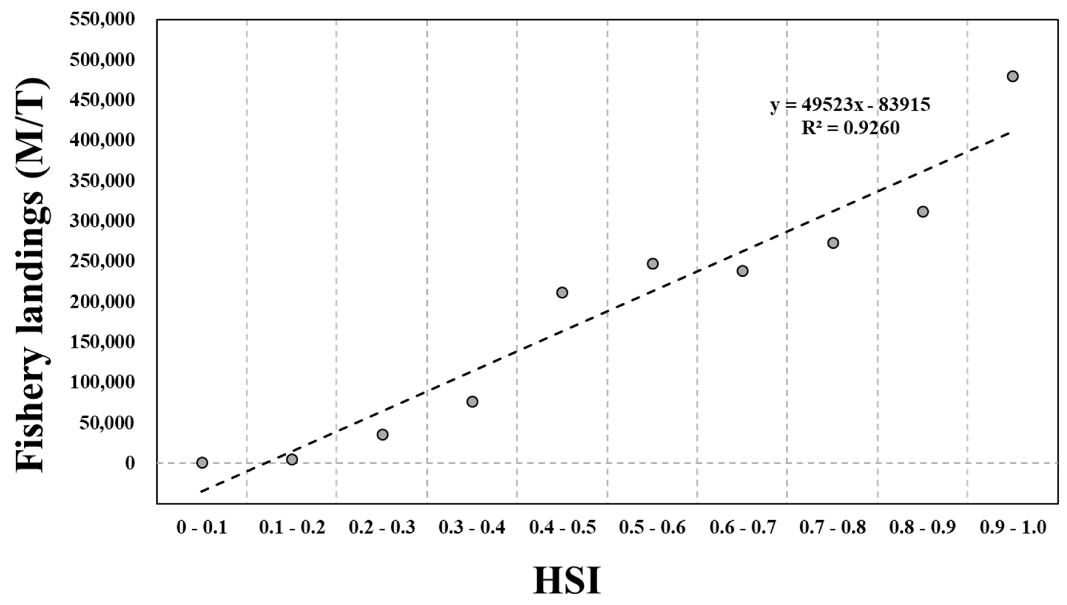
3.3. HSI Model Evaluation

To validate our HSI model, we compared the HSI values from our model with fishery catches. The HSI was divided into 10 classes with a step of 0.1. Then, we summed the landed fisheries from the region with the HSI values corresponding to each class. A strong positive linear relationship (R2 = 0.9260) was observed between the HSI and the fishery landings (Figure 8). In addition, spatial distributions between the HSI and the fish catches for the T. pacificus appeared well matched throughout 2010 to 2016 (Figure 9).

4. Discussion

4.1. Environmental Conditions

Among the several environmental variables, temperature and salinity are well known for the most important factors affect spatial and temporal distribution of marine fish species [40,41,42]. Several previous studies revealed the habitat formation is closely related with distribution of the SST, SSHA, Chl-a, and sea surface salinity (SSS) [14,16,39]. However, salinity was not considered in this study, since its variation in the East/Japan Sea and the South Sea mostly fell within the reported optimal ranges (from 31.93 to 35.7) [39] for the T. pacificus. Also, mixed layer depth (MLD) which can be a good indicator for the habitat formation of several species also not considered. The MLD dataset is hard to use in this study due to its relatively poor spatial. We need spatial resolution of at least 0.17 × 0.17 degrees due to the resolution of the catch data. Thus, the MLD is not considered in this study. Instead, we tried to examine the optimal conditions for the T. pacificus with other environmental variables.
The optimal environmental conditions for T. pacificus in this study showed similar results with several previous studies [5,39]. Alabia et al. [5] already reported that the environmental ranges of the potential squid habitat in the East/Japan Sea. According to them, the SST and the SSHA ranged from 10 to 30 °C and –0.16 to 0.36 cm, respectively, which correspond well with the results from our study. The Species Environmental Envelope (HSPEN) in AquaMaps global distribution model [39] also showed similar environmental range with this study. The species’ preferred environmental conditions for the T. pacificus in AquaMaps are 9.24–23.54 °C and 364–939 mg C m−2 d−1 for temperature and PP, respectively [39].
In this study, we tried to derive the HSI for the T. pacificus with SST, SSHA, Chl-a, and primary production around the South Korea. The habitat depth of T. pacificus is known to be at least 30 m and up to 100 m. It seems to be nonsense that HSI derivation for the T. pacificus with SST data, but the seasonal habitat distribution would be reflected in the range of SST. On the other hand, phytoplankton is not a direct prey of T. pacificus. However, the intermediate consumers in the food web can largely influenced by the distribution of phytoplankton [43]. Indeed, Lee et al. [44] already reported that the spatial distribution of the common minke whale (Balaenoptera acutorostrata) is closely related to the Chl-a distribution in the East/Japan Sea [44], although there is not any direct linkage in the food web. Moreover, the HSI derivation for the chub mackerel (Scomber japonicus) was also successfully conducted in the South Sea and the East/Japan Sea using primary production dataset [17]. As mentioned before, the zooplankton is an important food source for the juvenile T. pacificus and the small pelagic fishes which are main prey for the adult T. pacificus. Although there are only a few studies that have used primary production as an environmental variable for the HSI model, not only Chl-a but also primary production can be useful indicator of spatio-temporal distribution of the T. pacificus.
However, T. pacificus distributed mostly around South Korea and Japan (or northwestern pacific). Thus, the HSI model derived from regional dataset should be applied to global ocean or other regions carefully with understanding of the native distribution range of the target species.

4.2. Seasonal Variation of the HSI

In this study, seasonal variations of the HSI for the T. pacificus were observed which are not seen in map of the native habitat ranges. The optimal environmental conditions for the T. pacificus in this study showed high seasonal dependences. The optimum ranges of the SST and the SSHA for Summer–Autumn were significantly higher than those of Winter–Spring. The monthly distribution of the catches suggested that January and August are representative fishing time for each group (Figure 2). The catches occurred in January were mainly distributed in the southern part of the East/Japan Sea and the eastern part of the South Sea, while catches occurred in August mostly distributed in the Yellow Sea and the western part of the South Sea. As mentioned above, T. pacificus is well known for their characteristic migration routes around the Korean Peninsula. Also, they consist of two groups, the ‘winter spawners’ and ‘autumn spawners’. Their characteristic migration routes suggest that the caught population in January and August might be composed with different group each other. Consequently, the differences in the optimal environmental conditions between Summer–Autumn and Winter–Spring might be caused by these seasonal population distributions of T. pacificus in Korean waters.

4.3. Regions with High Catch Probability

For the investigation of the hotspots, which are the regions with high catch probability, we defined the hotspot as regions with an HSI over 0.7, because more than half of the total catches occurred in areas when the HSI ranged to 0.7 or more. The results of our hotspot analysis showed a seasonal distribution (Figure 10). One of the major hotspots was observed around the South Sea in winter (January–Febuary) and autumn (October–November). As mentioned above, not only the South Sea is well known for the spawning ground of the T. pacificus, they spawn during winter and autumn [2,3,4,5]. These characteristic spawning ground distributions of the T.pacificus might be reflected in the hotspot located in the South Sea. Another major hotspot located in the Yellow Sea was observed on July and September, while the hotspot located in the East/Japan Sea was observed on September and October. Generally, from late spring to early summer, the ‘winter spawners’ group begins to migrate mainly to the Yellow Sea which is well known for their feeding grounds, and their feeding activity continues until Autumn [3]. In case of the ‘autumn spawners’, they begin to migrate to the East/Japan Sea from spring to summer, and their feeding activity continues until late summer to autumn [3]. Consequently, the seasonal distribution of the hotspots was in agreement with the general migration patterns of the T. pacificus reported previously around the Korean Peninsula.

5. Summary and Conclusions

In this study, the HSI of the T. pacificus was derived by using commercial catch data and satellite datasets between 2010 and 2016. Four environmental parameters (SST, SSHA, Chl-a, and PP) were selected as key variables in the habitat formation of the T. pacificus.
The optimum environmental conditions for SST, SSHA, Chl-a, and PP were 14.91–27.26 °C, 0.05–0.20 m, 0.32–1.35 mg m−3, and 480.41–850.18 mg C m−2 d−1, respectively. More than 80% of the total catch obtained from the region within the optimum ranges. SST and SSHA showed high seasonality in frequency distributions (Figure 4). Based on these results, suitability index models for SST and SSHA were derived separately for winter to spring and summer to autumn (Figure 6). In the derivation of the HSI model, the AMM was used to combine the four SIs (SST, SSHA, Chl-a, and PP) since many previous studies reported that the AMM is the most appropriate model for marine fish species.
Based on the results from the HSI model, we found a strong positive relationship (R2 = 0.9260) between the HSI and the fishery landings (Figure 8) and good match for the spatial distributions of the T. pacificus (Figure 9). The seasonal variations of the spatial distribution of the HSI for the T. pacificus were observed in climatological monthly distribution of the HSI (Figure 7). In addition, the hotspot analysis the hotspot analysis revealed several major hotspots around the South Korea (Figure 10). The hotspot observed in the South Sea is consistent with the reported spawning grounds for T. pacificus. The hotspots observed in the Yellow Sea and the East/Japan Sea appear to be similar to the feeding grounds of the ‘winter spawners’ and ‘autumn spawners’, respectively. Consequently, the seasonal and spatial variations of the HSI match well with the migration patterns of the T. pacificus reported previously in the Korean waters. The HSI model derived from this study could help us to predict fishing grounds with high catch probability of the T. pacificus around South Korea. The monitoring of the HSI for the T. pacificus at the Yellow Sea and the East/Japan Sea can help us to successful fishery management. Ultimately, long-term analysis in spatial and temporal distributions of the HSI for the T. pacificus will allow us to understand the recent changes in fishery resources around South Korea.

Author Contributions

Conceptualization, D.L. and S.H.L.; data curation, D.L.; funding acquisition, C.-K.K. and S.H.L.; methodology, D.L.; project administration, C.-K.K. and S.H.L.; supervision, S.H.S. and S.H.L.; validation, D.L.; visualization, D.L.; writing—original draft, D.L.; writing—review and editing, S.H.S., C.-I.L., and S.H.L.

Funding

This research was supported by “Development of the integrated data processing system for GOCI-II” and and “Long-term change of structure and function in marine ecosystems of Korea” funded by the Ministry of Ocean and Fisheries, Korea.

Acknowledgments

The authors would like to thank the anonymous reviewers and the handling editors who dedicated their time for providing the authors with constructive and valuable recommendations.

Conflicts of Interest

The authors declare no conflict of interest.

References

  1. Korea Statistics; Korean Statistical Information Service (KOSIS). Fishery Production Survey; Korean Statistical Information Service (KOSIS): Daejeon, Korea, 2019. [Google Scholar]
  2. Kiyofuji, H.; Saitoh, S. Use of Nighttime Visible Images to Detect Japanese Common Squid Todarodes Pacificus Fishing Areas and Potential Migration Routes in the Sea of Japan. Mar. Ecol. Prog. Ser. 2004, 276, 173–186. [Google Scholar] [CrossRef]
  3. Kim, G.B.; Stapleton, H.M. PBDEs, Methoxylated PBDEs and HBCDs in Japanese Common Squid (Todarodes Pacificus) from Korean Offshore Waters. Mar. Pollut. Bull. 2010, 60, 935–940. [Google Scholar] [CrossRef] [PubMed]
  4. Waska, H.; Kim, G.; Kim, G.B. Comparison of S, Se, and 210 Po Accumulation Patterns in Common Squid Todarodes Pacificus from the Yellow Sea and East/Japan Sea. Ocean Sci. J. 2013, 48, 215–224. [Google Scholar] [CrossRef]
  5. Alabia, I.; Dehara, M.; Saitoh, S.; Hirawake, T. Seasonal Habitat Patterns of Japanese Common Squid (Todarodes Pacificus) Inferred from Satellite-Based Species Distribution Models. Remote Sens. 2016, 8, 921. [Google Scholar] [CrossRef]
  6. Park, C.; Kim, Y.; Park, J.; Kim, Z.; Choi, Y.; Lee, D.; Choi, K.; Kim, S.; Hwang, K. Ecology and Fishing Grounds of Major Commercial Fish Species in the Coastal and Offshore Korean Waters; National Fisheries Research and Development Institute Busan: Busan, Korea, 1998. (In Korean) [Google Scholar]
  7. Kang, Y.S.; Kim, J.Y.; Kim, H.G.; Park, J.H. Long-term Changes in Zooplankton and its Relationship with Squid, Todarodes Pacificus, Catch in Japan/East Sea. Fish. Oceanogr. 2002, 11, 337–346. [Google Scholar] [CrossRef]
  8. Jones, D.D.; Walters, C.J. Catastrophe Theory and Fisheries Regulation. J. Fish. Board Can. 1976, 33, 2829–2833. [Google Scholar] [CrossRef]
  9. Parmesan, C.; Yohe, G. A Globally Coherent Fingerprint of Climate Change Impacts Across Natural Systems. Nature 2003, 421, 37. [Google Scholar] [CrossRef]
  10. Perry, A.L.; Low, P.J.; Ellis, J.R.; Reynolds, J.D. Climate Change and Distribution Shifts in Marine Fishes. Science 2005, 308, 1912–1915. [Google Scholar] [CrossRef]
  11. Daskalov, G.M.; Grishin, A.N.; Rodionov, S.; Mihneva, V. Trophic Cascades Triggered by Overfishing Reveal Possible Mechanisms of Ecosystem Regime Shifts. Proc. Natl. Acad. Sci. USA 2007, 104, 10518–10523. [Google Scholar] [CrossRef]
  12. Brooks, R.P. Improving Habitat Suitability Index Models. Wildl. Soc. Bull. 1997, 25, 163–167. [Google Scholar]
  13. Morris, L.; Ball, D. Habitat Suitability Modelling of Economically Important Fish Species with Commercial Fisheries Data. ICES J. Mar. Sci. 2006, 63, 1590–1603. [Google Scholar] [CrossRef]
  14. Chen, X.; Li, G.; Feng, B.; Tian, S. Habitat Suitability Index of Chub Mackerel (Scomber Japonicus) from July to September in the East China Sea. J. Oceanogr. 2009, 65, 93–102. [Google Scholar] [CrossRef]
  15. Galparsoro, I.; Borja, Á.; Bald, J.; Liria, P.; Chust, G. Predicting Suitable Habitat for the European Lobster (Homarus Gammarus), on the Basque Continental Shelf (Bay of Biscay), using Ecological-Niche Factor Analysis. Ecol. Model. 2009, 220, 556–567. [Google Scholar] [CrossRef]
  16. Li, G.; Chen, X.; Lei, L.; Guan, W. Distribution of Hotspots of Chub Mackerel Based on Remote-Sensing Data in Coastal Waters of China. Int. J. Remote Sens. 2014, 35, 4399–4421. [Google Scholar] [CrossRef]
  17. Lee, D.; Son, S.; Kim, W.; Park, J.; Joo, H.; Lee, S. Spatio-Temporal Variability of the Habitat Suitability Index for Chub Mackerel (Scomber Japonicus) in the East/Japan Sea and the South Sea of South Korea. Remote Sens. 2018, 10, 938. [Google Scholar] [CrossRef]
  18. Rubec, P.J.; Bexley, J.C.; Norris, H.; Coyne, M.; Monaco, M.; Smith, S.; Ault, J. Suitability Modeling to Delineate Habitat Essential. Am. Fish. Soc. Symp. 1999, 22, 108–133. [Google Scholar]
  19. Vinagre, C.; Fonseca, V.; Cabral, H.; Costa, M.J. Habitat Suitability Index Models for the Juvenile Soles, Solea Solea and Solea Senegalensis, in the Tagus Estuary: Defining Variables for Species Management. Fish. Res. 2006, 82, 140–149. [Google Scholar] [CrossRef]
  20. Attrill, M.J.; Power, M. Climatic Influence on a Marine Fish Assemblage. Nature 2002, 417, 275. [Google Scholar] [CrossRef]
  21. Boeuf, G.; Payan, P. How should Salinity Influence Fish Growth? Com. Biochem. Physiol. C Toxicol. Pharmacol. 2001, 130, 411–423. [Google Scholar] [CrossRef]
  22. Pörtner, H.O.; Knust, R. Climate Change Affects Marine Fishes through the Oxygen Limitation of Thermal Tolerance. Science 2007, 315, 95–97. [Google Scholar] [CrossRef]
  23. Zainuddin, M.; Kiyofuji, H.; Saitoh, K.; Saitoh, S. Using Multi-Sensor Satellite Remote Sensing and Catch Data to Detect Ocean Hot Spots for Albacore (Thunnus Alalunga) in the Northwestern North Pacific. Deep Sea Res. II 2006, 53, 419–431. [Google Scholar] [CrossRef]
  24. Robinson, C.J.; Gómez-Gutiérrez, J.; de León, D.A.S. Jumbo Squid (Dosidicus Gigas) Landings in the Gulf of California Related to Remotely Sensed SST and Concentrations of Chlorophyll a (1998–2012). Fish. Res. 2013, 137, 97–103. [Google Scholar] [CrossRef]
  25. Tian, Y.; Akamine, T.; Suda, M. Variations in the Abundance of Pacific Saury (Cololabis Saira) from the Northwestern Pacific in Relation to Oceanic-Climate Changes. Fish. Res. 2003, 60, 439–454. [Google Scholar] [CrossRef]
  26. NASA Goddard Space Flight Center; Ocean Ecology Laboratory; Ocean Biology Processing Group. Moderate-Resolution Imaging Spectroradiometer (MODIS) Aqua 11µm Day/Night Sea Surface Temperature Data; 2018 Reprocessing; NASA OB.DAAC: Greenbelt, MD, USA, 2018. Available online: https://oceandata.sci.gsfc.nasa.gov/MODIS-Aqua/Mapped/Monthly/4km/sst/ (accessed on 11 September 2018). [CrossRef]
  27. NASA Goddard Space Flight Center; Ocean Ecology Laboratory; Ocean Biology Processing Group. Moderate-Resolution Imaging Spectroradiometer (MODIS) Aqua Chlorophyll Data; 2018 Reprocessing; NASA OB.DAAC: Greenbelt, MD, USA, 2018. Available online: https://oceandata.sci.gsfc.nasa.gov/MODIS-Aqua/Mapped/Monthly/4km/chlor_a/ (accessed on 11 September 2018). [CrossRef]
  28. NASA Goddard Space Flight Center; Ocean Ecology Laboratory; Ocean Biology Processing Group. Moderate-Resolution Imaging Spectroradiometer (MODIS) Aqua Photosynthetically Available Radiation Data; 2018 Reprocessing; NASA OB.DAAC: Greenbelt, MD, USA, 2018. Available online: https://oceandata.sci.gsfc.nasa.gov/MODIS-Aqua/Mapped/Monthly/4km/par/ (accessed on 11 September 2018). [CrossRef]
  29. NASA Goddard Space Flight Center; Ocean Ecology Laboratory; Ocean Biology Processing Group. Moderate-Resolution Imaging Spectroradiometer (MODIS) Aqua Downwelling Diffuse Attenuation Coefficient Data; 2018 Reprocessing; NASA OB.DAAC: Greenbelt, MD, USA, 2018. Available online: https://oceandata.sci.gsfc.nasa.gov/MODIS-Aqua/Mapped/Monthly/4km/Kd_490/ (accessed on 11 September 2018). [CrossRef]
  30. Behrenfeld, M.J.; Falkowski, P.G. Photosynthetic Rates Derived from satellite-based Chlorophyll Concentration. Limnol. Oceanogr. 1997, 42, 1–20. [Google Scholar] [CrossRef]
  31. Kirk, J.T. Light and Photosynthesis in Aquatic Ecosystems, 2nd ed.; Cambridge University Press: Cambridge, UK, 1994; pp. 129–169. [Google Scholar]
  32. Yamada, K.; Ishizaka, J.; Nagata, H. Spatial and Temporal Variability of Satellite Primary Production in the Japan Sea from 1998 to 2002. J. Oceanogr. 2005, 61, 857–869. [Google Scholar] [CrossRef]
  33. Yen, K.; Lu, H.; Chang, Y.; Lee, M. Using Remote-Sensing Data to Detect Habitat Suitability for Yellowfin Tuna in the Western and Central Pacific Ocean. Int. J. Remote Sens. 2012, 33, 7507–7522. [Google Scholar] [CrossRef]
  34. Chen, X.; Feng, B.; Xu, L. A Comparative Study on Habitat Suitability Index of Bigeye Tuna, Thunnus obesus in the Indian Ocean. J. Fish. Sci. China 2008, 15, 269–278. [Google Scholar]
  35. Grebenkov, A.; Lukashevich, A.; Linkov, I.; Kapustka, L.A. A habitat suitability evaluation technique and its application to environmental risk assessment. In Ecotoxicology, Ecological Risk Assessment and Multiple Stressors; Springer: Berlin/Heidelberg, Germany, 2006; pp. 191–201. [Google Scholar]
  36. Hess, G.R.; Bay, J.M. A Regional Assessment of Windbreak Habitat Suitability. Environ. Monit. Assess. 2000, 61, 239–256. [Google Scholar] [CrossRef]
  37. Lauver, C.L.; Busby, W.H.; Whistler, J.L. Testing a GIS Model of Habitat Suitability for a Declining Grassland Bird. Environ. Manag. 2002, 30, 88–97. [Google Scholar] [CrossRef]
  38. Van der Lee, G.E.M.; Van der Molen, D.T.; Van den Boogaard, H.F.P.; Van der Klis, H. Uncertainty Analysis of a Spatial Habitat Suitability Model and Implications for Ecological Management of Water Bodies. Landsc. Ecol. 2006, 21, 1019–1032. [Google Scholar] [CrossRef]
  39. Kaschner, K.; Kesner-Reyes, K.; Garilao, C.; Rius-Barile, J.; Rees, T.; Froese, R. AquaMaps: Predicted Range Maps for Aquatic Species; Version August 2016; World Wide Web Electronic Publication; Available online: www.aquamaps.org (accessed on 2 January 2019).
  40. Castillo, J.; Barbieri, M.; Gonzalez, A. Relationships between Sea Surface Temperature, Salinity, and Pelagic Fish Distribution off Northern Chile. ICES J. Mar. Sci. 1996, 53, 139–146. [Google Scholar] [CrossRef]
  41. Jaureguizar, A.J.; Menni, R.; Guerrero, R.; Lasta, C. Environmental Factors Structuring Fish Communities of the Rıo de la Plata Estuary. Fish. Res. 2004, 66, 195–211. [Google Scholar] [CrossRef]
  42. Sutcliffe, W., Jr.; Drinkwater, K.; Muir, B. Correlations of Fish Catch and Environmental Factors in the Gulf of Maine. J. Fish. Board Can. 1977, 34, 19–30. [Google Scholar] [CrossRef]
  43. Smith, R.; Dustan, P.; Au, D.; Baker, K.; Dunlap, E. Distribution of Cetaceans and Sea-Surface Chlorophyll Concentrations in the California Current. Mar. Biol. 1986, 91, 385–402. [Google Scholar] [CrossRef]
  44. Lee, D.; An, Y.R.; Park, K.J.; Kim, H.W.; Lee, D.; Joo, H.T.; Oh, Y.G.; Kim, S.M.; Kang, C.K.; Lee, S.H. Spatial Distribution of Common Minke Whale (Balaenoptera acutorostrata) as an Indication of a Biological Hotspot in the East Sea. Deep Sea Res. II 2017, 143, 91–99. [Google Scholar] [CrossRef]
Figure 1. Summarized commercial catch data for the T. pacificus during 2010 to 2016.
Remotesensing 11 02720 g001
Figure 2. Monthly distribution of total fishery landings (M/T) and the number of fishing records.
Remotesensing 11 02720 g002
Figure 3. Distribution of the suitability index of (a) sea surface temperature (SST) (°C), (b) sea surface height anomaly (SSHA) (m), (c) chlorophyll-a (Chl-a) (mg m−3), and (d) primary production (PP) (mg C m−2 d−1) on the fishing locations for the T. pacificus. Gray square represents an optimum range for each parameter.
Remotesensing 11 02720 g003
Figure 4. Seasonal distributions of suitability index for the SST (°C) and SSHA (m) on the fishing locations for the T. pacificus.
Remotesensing 11 02720 g004
Figure 5. Seasonality of frequency distributions of SST (°C) and SSHA (m) on the fishing locations for the T. pacificus.
Remotesensing 11 02720 g005
Figure 6. Least squares fitting results of (a) SST (°C), (b) SSHA (m), (c) Chl-a (mg m−3), and (d) PP (mg C m−2 d−1) with the number of fishing sets (solid line: habitat suitability index (HSI) model, black dot: in situ fishing data).
Remotesensing 11 02720 g006
Figure 7. Climatological monthly distribution of the (HSI) around South Korea from 2002 to 2016.
Remotesensing 11 02720 g007
Figure 8. Correlation between the HSI and the fishery landings. Fishery landings were summed in each range of the HSI value.
Remotesensing 11 02720 g008
Figure 9. Spatial distribution of the eight-day composited HSI and the T. pacificus catches (black open circle) at corresponding periods in the South Sea.
Remotesensing 11 02720 g009
Figure 10. Climatological monthly distribution of the HSI hotspots (HSI > 0.7) for the T. pacificus around South Korea from 2002 to 2016.
Remotesensing 11 02720 g010
Table 1. The number of commercial catch data matched with satellite datasets.
YearReported CatchesNo. of Matchable Catches
2010797486
20111593956
20121479918
20131372834
20141219775
201516401099
20161301892
Total94015960
Table 2. SI models derived from three environmental parameters (SST, SSHA, Chl-a, and PP).
VariablesSI modelsRMSER2
SSTWSexp(−0.2929(XSST − 15.44)2)0.05000.9654
SSTSAexp(−0.0657(XSST − 24.22)2)0.07450.9461
SSHAWSexp(−184.8(XSST + 0.01325)2)0.08710.9063
SSHASAexp(−157(XSST − 0.1514)2)0.06670.9468
Chl-aexp(−16.98(ln(XChl) + 0.5997)2)0.06400.9165
PPexp(−0.00004637(XPP − 658.7)2)0.08760.9072

