Article

Annual Green Water Resources and Vegetation Resilience Indicators: Definitions, Mutual Relationships, and Future Climate Projections

1
European Commission, Joint Research Centre, 21027 Ispra, Italy
2
Fondazione Centro euro-Mediterraneo sui Cambiamenti Climatici—CMCC, 40127 Bologna, Italy
3
Faculty ITC, University of Twente, 7500 AE Enschede, The Netherlands
*
Author to whom correspondence should be addressed.
Remote Sens. 2019, 11(22), 2708; https://doi.org/10.3390/rs11222708
Submission received: 25 October 2019 / Accepted: 15 November 2019 / Published: 19 November 2019
(This article belongs to the Special Issue Ecosystem Services with Remote Sensing)

Abstract

:
Satellites offer a privileged view on terrestrial ecosystems and a unique possibility to evaluate their status, their resilience and the reliability of the services they provide. In this study, we introduce two indicators for estimating the resilience of terrestrial ecosystems from the local to the global levels. We use the Normalized Differential Vegetation Index (NDVI) time series to estimate annual vegetation primary production resilience. We use annual precipitation time series to estimate annual green water resource resilience. Resilience estimation is achieved through the annual production resilience indicator, originally developed in agricultural science, which is formally derived from the original ecological definition of resilience i.e., the largest stress that the system can absorb without losing its function. Interestingly, we find coherent relationships between annual green water resource resilience and vegetation primary production resilience over a wide range of world biomes, suggesting that green water resource resilience contributes to determining vegetation primary production resilience. Finally, we estimate the changes of green water resource resilience due to climate change using results from the sixth phase of the Coupled Model Inter-comparison Project (CMIP6) and discuss the potential consequences of global warming for ecosystem service reliability.

Graphical Abstract

1. Introduction

The contribution of ecosystems to human well-being has received growing attention in the public and scientific domains. Following the multilateral treaty of the 1992 International Convention on Biological Diversity of the United Nations, the 2010 Conference of Parties (COP 10) formally engaged on a strategic plan to “take effective and urgent action to halt the loss of biodiversity in order to ensure that by 2020 ecosystems are resilient and continue to provide essential services”, explicitly recognizing the need for resilient ecosystems, able to withstand the increasing pressure from climate change and anthropization. More recently, in 2015, world leaders adopted the Sustainable Development Goals (SDG), which among others include climate action (SDG13) and life on land (SDG 15) to ensure conservation and restoration of vegetation and sustainable use of the related ecosystems services [1].
The scientific community has provided evidence on the key role of ecosystems for human well-being [2], and has discussed the economic valuation of ecosystem services to mainstream their value into the decision-making process, with the intent to support their conservation, restoration and sustainable use [3,4,5]. The assessment and valuation of ecosystem services and their changes over time have been the focus of many scientific studies and projects from the global [6,7] to the regional [8,9] and the local scale [10]. Terrestrial ecosystems in good ecological status have been found to [5]:
  • Protect from erosion and landslides.
  • Protect from inland flooding.
  • Buffer natural resources against drier and more variable climates.
  • Reduce risks and impacts of wildfires.
  • Protect from coastal hazards and sea level rise.
  • Moderate urban heatwaves and heat island effects.
  • Managing stormwater and flooding in urban areas.
However, how to measure terrestrial ecosystems’ ecological status and their ability to withstand the increasing pressure of climate change and anthropization—i.e., their resilience—is still an open question.
Data from satellite remote sensing have been increasingly adopted for assessing vegetation resilience and ecosystem services, as they can provide information on the land cover typology, extent and characteristics at different points in time, and from the local to the global scale [11,12]. Remotely sensed data can be used to define vegetation indexes such as the Normalized Difference Vegetation Index (NDVI) that is strongly correlated with the photosynthetic activity of the plant canopies [13]. The NDVI is frequently used to assess ecological responses of vegetation to climatic conditions and environmental changes [12,14,15] and has often been adopted as proxy for ecosystem services [16,17,18,19,20].
The NDVI was used as a key indicator in a wide range of ecosystem services including (according to the Millennium Ecosystem Assessment classification): provisioning services, such as energy, food, raw materials, water provisioning, and genetic resources; regulating services, such as climate regulation, disturbance regulation, erosion regulation, flood regulation, hazard regulation, pollination, water purification, and waste treatment; supporting services, such as biological refugia, habitat, primary production in sea and rivers; cultural ecosystem services, such as cultural heritage and recreation [21].
Until recently the focus has been mainly on the assessment of the current flow of ecosystem services and their relative changes compared to past conditions [6,22], which has been possible by the availability of satellite data time series. Given the importance of ecosystem resilience for the reliability of the provided services, several studies have addressed the resilience of ecosystems through indicators of ecosystem stability [23,24]. However, additional research is needed to quantify the resilience of ecosystems to environmental change in spatially explicit assessments [25].
Here, we focus on the estimation of terrestrial ecosystem resilience related to the stability of primary production, which is generally recognized as one of the main constituent of ecosystem resilience [26]. We estimate vegetation primary production resilience by means of the NDVI and its inter-annual variability. More specifically, we adopt the recently proposed indicator for annual crop production resilience [27]. This indicator is derived from the original ecological definition of resilience i.e., the measure of the largest stress that the system can absorb without losing its function [28]. We apply the annual resilience indicator to remotely sensed NDVI, as proxy of vegetation primary production. Furthermore, we apply the annual resilience indicator to ground-based precipitation data, as proxy of annual green water resources (i.e., the water available to plants [29]).
We show and discuss three main results.
  • Validity of the fundamental principle of the resilience indicator [27] applied to precipitation, i.e., its proportionality with drought return times.
  • Relationship between the water resource resilience indicator and the vegetation primary production resilience.
  • Changes of green water resource resilience due to global warming.

2. Materials and Methods

The original meaning of the term resilience—first introduced in ecology—refers to the largest pressure that a system can cope with without changing its internal structure and losing its functioning capacity [28,30]. While the concept of resilience has evolved in complexity while spreading into other fields such as engineering and social sciences, a recent study [27] brought back the original ecological definition of resilience. The only assumption of that study is that severe shocks are rarer than moderate perturbances. This allows measuring the severity of the shock by its return period and to formally derive a consistent statistical indicator that can be computed on annual production time series [27]. This section summarizes the main properties of the resilience indicator (RC) and introduces its application to NDVI and precipitation data.

2.1. Annual Crop Production Resilience Indicator (RC): Definition and Properties

The resilience indicator for annual crop production [27] is defined as the squared mean divided by the squared standard deviation of annual production time series:
RC = μ2/σ2,
It has been demonstrated [27] that the RC indicator provides several advantages:
  • It is formally derived from the ecological definition of resilience, thus, theoretically more grounded than similar indicators based on different functions of the μ over σ ratio such as the coefficient of variance.
  • It is inversely/directly proportional to the frequency / return period of the extreme events leading to large production losses.
  • It takes into account spatial heterogeneities and diversity in a simple and intuitive manner i.e., RC computed on the sum of n uncorrelated time series with same μ and σ is exactly n-times RC of the individual time series.
  • It is simple to compute, and it can take into account the effects of non-linear long-term trends easily e.g., by normalizing the time series by the running mean baseline values prior to the indicator computation.
Unfortunately, RC suffers from the disadvantage of requiring relatively long time series for an accurate estimation of resilience. For normally distributed variables, a sample size over 30 values is typically needed to compute RC with and accuracy of 30% [27].

2.2. Annual Green Water Resources Resilience Indicator (RP): Definition and Data

The annual green water resources resilience indicator (RP) follows the same formulation as the RC indicator (Equation (1)) but it is computed using annual precipitation data i.e., the main input variable that defines the so-called green water [29]. In this work, we use global precipitation data since 1901 at half-degree spatial resolution from the Climate Research Unit (CRU) archive [31].
We test the rationale behind the RC indicator applied on precipitation (i.e., point 2 of Section 2.1) by comparing RP values to the frequency of meteorological drought estimated independently with the Weighted Anomaly of Standardized Precipitation (WASP) index [32,33] (i.e., the same data used in Figure 3 of Carrão et al.’s paper [33]).
To provide a preliminary estimate of future change of water resource resilience due to climate change, we compute RP using data from the sixth phase of the Coupled Model Inter-comparison Project (CMIP6). At the time this analysis has been developed, climate change simulations performed by six climate models (CanESM5, CNRM-CM6, IPSL-CM6A-LR, MIROC6, MRI-ESM2-0 and UKESM1-0-LL) were available for the historical period (1850–2014) and Shared Socio-economic Pathways SSP585 [34] for period 2015–2100. The SSP585 corresponds to a high emissions scenario consistent with the Representative Concentration Pathway RCP 8.5 used in CMIP5.

2.3. Annual Vegetation Primary Production Resilience Indicator (RV): Definition and Data

The annual vegetation primary production resilience indicator (RV) is analog to the RC indicator (Equation (1)) but it is computed using annual NDVI data, which we use as proxy of gross primary production. NDVI time series spanning the period July 1981 to December 2015 were obtained from the Global Inventory Modeling and Mapping Studies(GIMMS) NDVI3g v1 dataset [35]. The long-term GIMMS dataset is derived from measurements made by different Advanced Very High Resolution Radiometer (AVHRR) sensors on board of the National Oceanic and Atmospheric Administration (NOAA) polar-orbiting satellite series [35]. The satellite observations are corrected for various effects, including sensor degradation, orbital drift, atmospheric effects, and volcanic eruptions. The time series have a temporal resolution of about 15 days (i.e., two observations per month, one referring to day 1–15 and one to day 16-end of the month) and a spatial resolution of 1/12 degree. The 15-day composites were obtained using the maximum value composition (MVC) technique [36], which minimizes the scattering and absorption effects of the atmosphere.
We temporally smoothed the time series to reduce remaining noise. We applied an iterative Savitzky–Golay filter [37] to fit the upper envelope of the NDVI time profiles as described by Chen et al. [38]. Finally, the annual mean NDVI values were calculated for the period 1982–2015.
We aggregate the NDVI data at 0.5-degree resolution to allow analyzing the relationship between RV and RP. Water bodies are not considered in the aggregated values, which are achieved through a conservative mapping procedure [39]. We discuss the relationships between RV and RP for each world biomes grouping the results by homogeneous climatic areas according to the Köppen–Geiger (KG) classification [40]. The KG classification codes are listed in Table 1.

2.4. Properties of RP and RV

The RP and RV indicators inherit all properties of RC (Section 2.1). In addition, the RP and RV indicators computed at the grid cell level have an important property, i.e., they neither depend on the period of the year nor on the portion of area with no precipitation or vegetation within the analyzed cell (P = 0, NDVI close to 0).
Assuming linear mixing, this claim can be proven by computing the mean and the variance of a time series of values xi, i = 1,.., N and of derived values defined as yi = a × xi, where a is the fraction of area or the fraction of period where precipitation or NDVI are not null. It follows that μy = a × μx and σy = a × σx, so the resilience indicator computed on these two time series does not change (q.e.d.). Please note that if a trend exists in the period of the year or portion of area with no precipitation or vegetation, this should be removed as mentioned in point 4 of Section 2.1.
Because of the 3rd property of the resilience indicator (Section 2.1), when aggregating the resilience indicator computed at the grid cell level over an area of interest, the resulting resilience will be larger if groups of temporally uncorrelated (i.e., diverse) cells exist in the area.

3. Results

The three main findings of this study are here shown and discussed:
  • The test of the annual resilience indicator applied to precipitation to be inversely proportional to drought frequency (Section 3.1–2nd property).
  • The relationship between RP and RV (Section 3.2).
  • The effects of climate change on RP (Section 3.3).

3.1. Annual Green Water Resources Resilience Indicator (RP) and Drought Frequency Since 1901

Figure 1 shows the mean (Figure 1a), the standard deviation (Figure 1b) of observed annual precipitation data since 1901, as well as their combination defining RP (Figure 1c). RP tends to be larger in regions with high precipitation values. However, the spatial variability is larger than the one of the precipitation magnitude due to complex patterns of precipitation inter-annual variability. Inter-annual variability is probably underestimated in regions with scarce data such as central Greenland, Western Arabian Peninsula, and Central Amazon Forest, hindering the accurate computation of the annual green water resource resilience indicator.
Figure 1d shows the drought hazard computed as the probability of exceeding the median of global severe precipitation deficits for the reference period using the WASP [32]). The data displayed in Figure 1d is exactly the same as in Figure 3 of [33] and shows the frequency of abnormal precipitation deficits defining drought prone regions. Comparison between Figure 1c,d strongly suggests an inverse relationship between RP and drought frequency.
Figure 2 shows the relationship between RP and drought return periods. Their joint distribution is consistent, despite the large scatter of the data, with a global tendency toward the increase of drought return periods with increasing values of the precipitation resilience indicator. This consistency was tested using the proportionality coefficient that we found to be statistically significant with a p-value < 0.001.

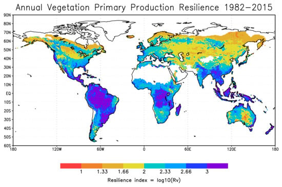
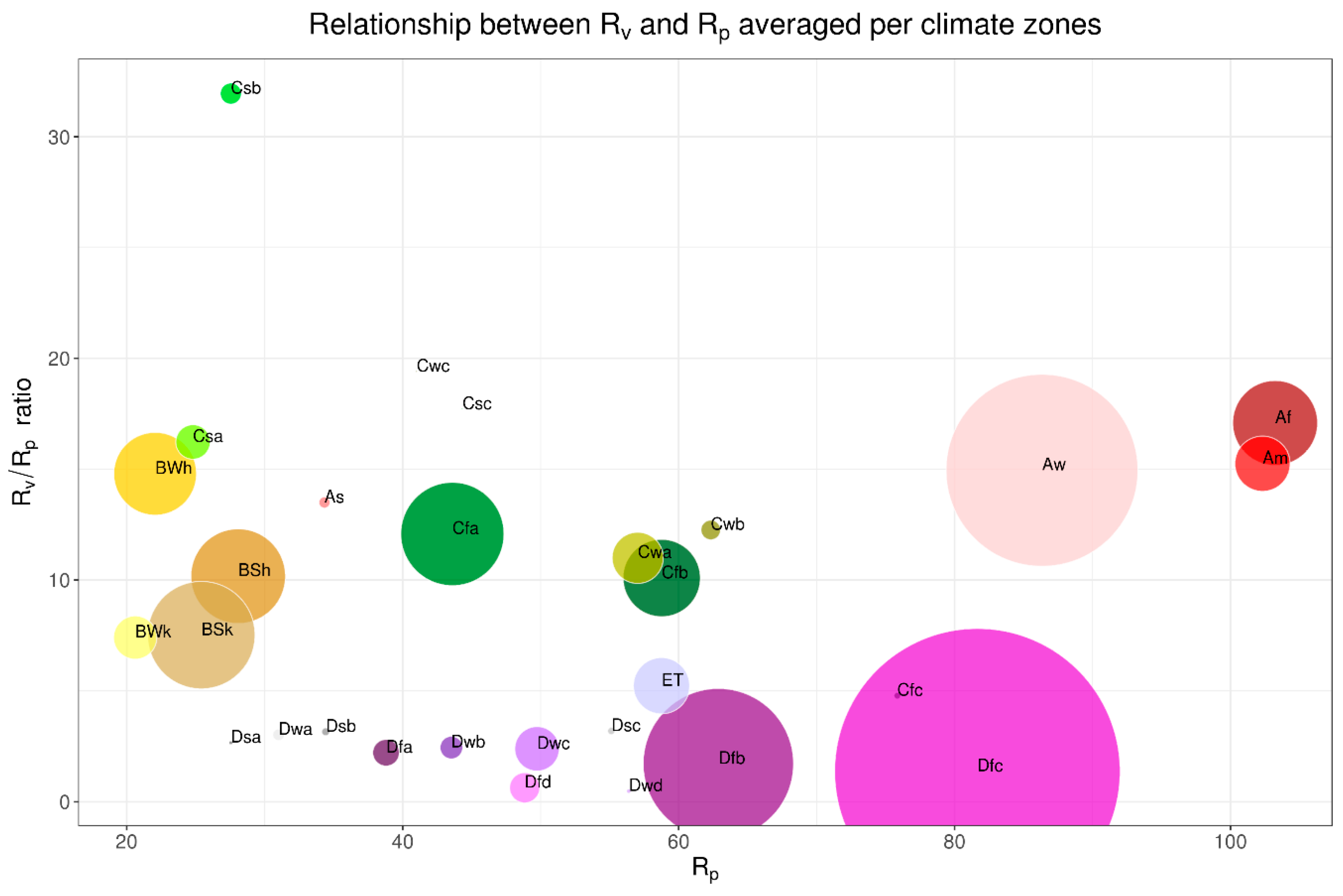
3.2. Precipitation and Vegetation Resilience Indicator Since 1982

Figure 3 shows the mean (Figure 3a), the standard deviation (Figure 3b) of annual mean NDVI data since 1982, as well as their combination defining RV (Figure 3c). RV is larger in tropical regions, where the NDVI is large and the inter-annual variability is relatively low. RV sharply decreases in subtropical regions, characterized by large inter-annual NDVI variability. RV also decreases towards the high latitudes, where vegetation is generally less vigorous and subject to the largest inter-annual variability.
Table 2 shows the overall statistics organized per Köppen–Geiger (KG) classification. In general, RV tends to be larger than RP. We note a relatively large spread of the precipitation data, i.e., large standard deviation with respect to the mean precipitation averaged in each KG climate zone. The spread of the drought frequency estimate by the WASP and the vegetation data measured by the NDVI is smaller. The latter result is somehow expected because the KG climate classification was developed exactly to characterize homogeneous land ecosystems. The spread of the green water resources and vegetation primary production resilience indicators over homogeneous climate zones is also relatively large, probably reflecting the dependency of the resilience indicator accuracy computed on time series of limited length [23,27].
However, the mean RV is often significantly different among KG classes. RP is higher in equatorial (A class) and warm temperate climates (C class) than in arid climate (B class). Similarly, RV decreases from equatorial (A class) to warm temperate (C class), arid (B class) and snow (D class) climates. Within warm temperate biomes (C class), RP is greater in fully humid (f class) than in winter and summer dry regions (w and s classes, respectively), while RV takes higher values in winter dry and summer dry (with warm summer) climates (wb and sb classes, respectively) rather than in fully humid climates (f class). In arid climates (B class), RP is greater in the steppe than in the desert regions (S and W classes respectively), while lower values of RV are found in cold areas than in hot areas (class k and h respectively). In snow climates (class D), regions with cool and warm summer (class c and b) have higher RV than regions with hot summer or extremely continental weather (a and d classes, respectively).
The size of the markers represents the land area actually covered by the homogeneous climate zones. The color scheme is the same as in Figure 4d.
Figure 4 shows the relationships between RP and RV averaged over the climate zones defined according to the Köppen–Geiger classification (Table 2).
Despite the large scatter of the data that emerged from the analysis in Table 2, the comparison between RP and RV for different climate zones displays clear relationships. In fact, the ratio between the two is roughly constant over two wide ranges of biomes. On the one hand, the RV/RP ratio tends to stay around the 10–15 band for ecosystems ini arid climate (i.e., the B class), warm temperate climate (C class) and equatorial climate (A class). On the other hand, the RV/RP ratio tends to stay below 5 for snow and polar climates (i.e., the “D” and E classes, respectively) as well as the subpolar oceanic climate (Cfc), representing an exception to the previous statement. Another exception is represented by the warm-summer Mediterranean climate (Csb), characterized by the largest RV/RP ratio. This peculiar climate is found in the north-western Iberian Peninsula and central Anatolia (see Figure 3d).

3.3. Effects of Climate Change on Annual Green Water Resources Resilience Indicator (RP)

Figure 5 shows the changes in mean annual precipitation (Figure 5a), standard deviation (Figure 5b) and of RP (Figure 5c) computed from an ensemble of six climate models from CMIP6 between the periods 1981–2014 and 2015–2100. The mean annual precipitation and the standard deviation are increasing in many regions around the globe and mainly in the Northern Hemisphere, because of the larger humidity levels that the warmer atmosphere can hold, because of alterations in the frequencies of large-circulation patterns and because of the general increase of climate variability [41,42]. According to these simulations, the relative ratio of the increases in the mean and in the standard deviation of annual precipitation is such that the annual RP is decreasing over most regions (Figure 5c,d). Despite the generalized increase in precipitation, the significant increase in inter-annual variability is reflected in a reduction of RP over most regions around the globe. This means that even though there will be more water available, this will be less reliable. The only exception is found in desert regions, where small increases in mean precipitation are dominating the RP signal.

4. Discussion

The functional quality of ecosystems is directly linked to the amount and reliability of services they can provide [43,44]. With this paper, we enrich the set of analysis tools for assessing the quality and the stability of ecosystems through the resilience indicators that we propose to apply to green water resources and to vegetation primary production.
These indicators, formally derived from the ecological definition of resilience [27], require relatively long time series (30 years and more) that, despite not available from the most frequently used satellite mission (e.g., MODIS, SPOT-VGT and Prob-V), can be extracted from AVHRR-based long-term archive as the one used in this study (i.e., GIMMS). This long-term approach may thus complement more complex resilience measures based on the engineering definition of resilience i.e., the ecosystem recovery time more suited for short time-scales analyses [45,46]. Comparing these two different views would probably provide an interesting way forward to the understanding of ecosystems resilience and stability assessments.
Our analysis linking annual precipitation and vegetation productivity suggests a coherent relationship between the resilience indicators computed on precipitation and NDVI. The magnitude of the resilience indicator for vegetation was found larger than the one of precipitation. This may indicate the capability of vegetated ecosystems to maintain their functioning also in the presence of precipitation variability. Nevertheless, the spatial patterns of the two resilience indicators do coincide to a great extent. In regions with reduced agreement, as for instance in the high latitudes of the Northern Hemisphere, the reduced vegetation resilience as compared to the precipitation resilience may be due to temperature and/or radiation, not explicitly considered in this study. Further studies are needed to assess the robustness of these results including, for instance, the effects of temperature and radiation as well.
This analysis could also be further evolved by accounting for the delay between precipitation input and vegetation response, as well as different time-scales [45,47,48], including different seasonalities such as double seasons and different periodicities as those found in the Southern Hemisphere and disentangling the differences between natural and anthropic vegetation cover, possibly isolating the effects of management and irrigation [49].

5. Conclusions

This paper provides an alternative framework for the assessment of ecosystem resilience by proposing two indicators, one for green water resources and one for vegetation productivity, based on the ecological definition of resilience [27].
Our global scale analysis strongly suggests a coherent relationship between these indicators over two wide ranges of biomes in the present climate. However, further studies are needed to quantify the robustness of these relationships in a changing climate, considering other definitions of resilience as well [23,45]. Including temperature and radiation would be also needed to fully explain the observed spatial patterns in vegetation resilience.
Quantifying the resilience of ecosystems and ecosystem services is of upmost relevance when considering future climate change [50,51,52,53]. Indeed, the variation of temperature and precipitation patterns caused by climate change is expected to affect the availability and seasonality of water resources and the growing season of vegetation in various regions of the world [54], affecting biodiversity and the provisioning of ecosystem services [24,46,55].
Our preliminary analysis of climate change projections from CMIP6 data displays alarming results. The increase of precipitation magnitude projected for the next future is counterbalanced by the concomitant increase of its variability, resulting in a general decrease of green water resource resilience at the global level.
In the future, it would also be interesting to carry on this analysis with an indicator of Blue Water Resources Resilience, which could be easily defined by computing the resilience indicator on the surface water budget given by precipitation minus evapotranspiration. This could be put in relation with soil moisture and river drought through the standardized Precipitation Evapotranspiration Index (SPEI [56,57]) or the Standardized River Discharge Index (SRDI [58,59]) to measure the reliability of freshwater resources for society and to help assessing the status of river ecosystems [60]. This additional resilience indicator may be potentially suitable for river related ecosystem services.

Author Contributions

Conceptualization, methodology, and formal analysis, M.Z.; data curation, M.M., E.S., A.V. and G.N.; visualization, M.Z and G.N; writing—original draft preparation, M.Z. and B.G.; writing—review and editing, M.Z., B.G., M.M., E.S., A.V., G.N. and A.T.

Funding

This research received no external funding.

Conflicts of Interest

The authors declare no conflict of interest.

References

  1. United Nations Economic and Social Council. Report of the Inter-Agency and Expert Group on Sustainable Development Goal Indicators. In Proceedings of the Statistical Commission Forty-Seventh Session, New York, NY, USA, 8–11 March 2016. [Google Scholar]
  2. Millennium Ecosystem Assessment. Ecosystems and Human Well-Being: Synthesis; Island Press: Washington, DC, USA, 2005. [Google Scholar]
  3. The Economics of Ecosystems and Biodiversity. Ecological and Economic Foundation; Routledge: London, UK, 2010. [Google Scholar]
  4. Davis, A.S.; Hill, J.D.; Chase, C.A.; Johanns, A.M.; Liebman, M. Increasing Cropping System Diversity Balances Productivity, Profitability and Environmental Health. PLoS ONE 2012, 7, e47149. [Google Scholar] [CrossRef] [PubMed]
  5. Seddon, N.; Turner, B.; Berry, P.; Chausson, A.; Girardin, C.A.J. Grounding nature-based climate solutions in sound biodiversity science. Nat. Clim. Chang. 2019, 9, 84–87. [Google Scholar] [CrossRef]
  6. Costanza, R.; de Groot, R.; Sutton, P.; van der Ploeg, S.; Anderson, S.J.; Kubiszewski, I.; Farber, S.; Turner, R.K. Changes in the global value of ecosystem services. Glob. Environ. Chang. 2014, 26, 152–158. [Google Scholar] [CrossRef]
  7. Pascual, U.; Balvanera, P.; Díaz, S.; Pataki, G.; Roth, E.; Stenseke, M.; Watson, R.T.; Başak Dessane, E.; Islar, M.; Kelemen, E.; et al. Valuing nature’s contributions to people: The IPBES approach. Curr. Opin. Environ. Sustain. 2017, 26–27, 7–16. [Google Scholar] [CrossRef]
  8. Maes, J.; Liquete, C.; Teller, A.; Erhard, M.; Paracchini, M.L.; Barredo, J.I.; Grizzetti, B.; Cardoso, A.; Somma, F.; Petersen, J.-E.; et al. An indicator framework for assessing ecosystem services in support of the EU Biodiversity Strategy to 2020. Ecosyst. Serv. 2016, 17, 14–23. [Google Scholar] [CrossRef]
  9. Santos-Martín, F.; Zorrilla-Miras, P.; Palomo, I.; Montes, C.; Benayas, J.; Maes, J. Protecting nature is necessary but not sufficient for conserving ecosystem services: A comprehensive assessment along a gradient of land-use intensity in Spain. Ecosyst. Serv. 2019, 35, 43–51. [Google Scholar] [CrossRef]
  10. Dunford, R.; Harrison, P.; Smith, A.; Dick, J.; Barton, D.N.; Martin-Lopez, B.; Kelemen, E.; Jacobs, S.; Saarikoski, H.; Turkelboom, F.; et al. Integrating methods for ecosystem service assessment: Experiences from real world situations. Ecosyst. Serv. 2018, 29, 499–514. [Google Scholar] [CrossRef]
  11. Shi, L.; Wang, Y.; Jia, Y.; Lu, C.; Lei, G.; Wen, L. Vegetation Cover Dynamics and Resilience to Climatic and Hydrological Disturbances in Seasonal Floodplain: The Effects of Hydrological Connectivity. Front. Plant Sci. 2017, 8, 2196. [Google Scholar] [CrossRef]
  12. Cui, X.; Gibbes, C.; Southworth, J.; Waylen, P. Using Remote Sensing to Quantify Vegetation Change and Ecological Resilience in a Semi-Arid System. Land 2013, 2, 108–130. [Google Scholar] [CrossRef]
  13. Myneni, R.B.; Keeling, C.D.; Tucker, C.J.; Asrar, G.; Nemani, R.R. Increase plant growth in the northern high latitudes from 1981 to 1991. Nature 1997, 386, 698–702. [Google Scholar] [CrossRef]
  14. Pettorelli, N.; Vik, J.O.; Mysterud, A.; Gaillard, J.; Tucker, C.J.; Stenseth, N.C.; Lyon, C.B. Using the satellite-derived NDVI to assess ecological responses to environmental change. Trends Ecol. Evol. 2005, 20, 503–510. [Google Scholar] [CrossRef] [PubMed]
  15. Hilker, T.; Lyapustin, A.I.; Tucker, C.J.; Hall, F.G.; Myneni, R.B.; Wang, Y.; Bi, J.; de Moura, Y.; Sellers, P.J. Vegetation dynamics and rainfall sensitivity of the Amazon. Proc. Natl. Acad. Sci. USA 2014, 111, 16041–16046. [Google Scholar] [CrossRef] [PubMed]
  16. Krishnaswamy, J.; Bawa, K.S.; Ganeshaiah, K.N.; Kiran, M.C. Quantifying and mapping biodiversity and ecosystem services: Utility of a multi-season NDVI based Mahalanobis distance surrogate. Remote Sens. Environ. 2009, 113, 857–867. [Google Scholar] [CrossRef]
  17. Roces-Díaz, J.V.; Díaz-Varela, R.A.; Álvarez-Álvarez, P.; Recondo, C.; Díaz-Varela, E.R. A multiscale analysis of ecosystem services supply in the NW Iberian Peninsula from a functional perspective. Ecol. Indic. 2015, 50, 24–34. [Google Scholar] [CrossRef]
  18. Paruelo, J.M.; Texeira, M.; Staiano, L.; Mastrángelo, M.; Amdan, L.; Gallego, F. An integrative index of Ecosystem Services provision based on remotely sensed data. Ecol. Indic. 2016, 71, 145–154. [Google Scholar] [CrossRef]
  19. Calderón-Contreras, R.; Quiroz-Rosas, L.E. Analysing scale, quality and diversity of green infrastructure and the provision of Urban Ecosystem Services: A case from Mexico City. Ecosyst. Serv. 2017, 23, 127–137. [Google Scholar] [CrossRef]
  20. De Carvalho, R.M.; Szlafsztein, C.F. Urban vegetation loss and ecosystem services: The influence on climate regulation and noise and air pollution. Environ. Pollut. 2019, 245, 844–852. [Google Scholar] [CrossRef]
  21. De Araujo Barbosa, C.C.; Atkinson, P.M.; Dearing, J.A. Remote sensing of ecosystem services: A systematic review. Ecol. Indic. 2015, 52, 430–443. [Google Scholar] [CrossRef]
  22. Liquete, C.; Udias, A.; Conte, G.; Grizzetti, B.; Masi, F. Integrated valuation of a nature-based solution for water pollution control. Highlighting hidden benefits. Ecosyst. Serv. 2016, 22, 392–401. [Google Scholar] [CrossRef]
  23. De Keersmaecker, W.; Lhermitte, S.; Honnay, O.; Farifteh, J.; Somers, B.; Coppin, P. How to measure ecosystem stability? An evaluation of the reliability of stability metrics based on remote sensing time series across the major global ecosystems. Glob. Chang. Biol. 2014, 20, 2149–2161. [Google Scholar] [CrossRef]
  24. Oliver, T.H.; Isaac, N.J.B.; August, T.A.; Woodcock, B.A.; Roy, D.B.; Bullock, J.M. Declining resilience of ecosystem functions under biodiversity loss. Nat. Commun. 2015, 6, 10122. [Google Scholar] [CrossRef] [PubMed]
  25. Maes, J.; Egoh, B.; Willemen, L.; Liquete, C.; Vihervaara, P.; Schägner, J.P.; Grizzetti, B.; Drakou, E.G.; Notte, A.L.; Zulian, G.; et al. Mapping ecosystem services for policy support and decision making in the European Union. Ecosyst. Serv. 2012, 1, 31–39. [Google Scholar] [CrossRef]
  26. Brandl, S.J.; Rasher, D.B.; Côté, I.M.; Casey, J.M.; Darling, E.S.; Lefcheck, J.S.; Duffy, J.E. Coral reef ecosystem functioning: Eight core processes and the role of biodiversity. Front. Ecol. Environ. 2019, 17, 445–454. [Google Scholar] [CrossRef]
  27. Zampieri, M.; Weissteiner, C.; Grizzetti, B.; Toreti, A.; Van Den Berg, M.; Dentener, F. Estimating resilience of annual crop production systems: Theory and limitations. arXiv 2019, arXiv:1902.02677. [Google Scholar]
  28. Holling, C.S. Resilience and stability of ecological systems. Annu. Rev. Ecol. Syst. 1973, 4, 1–23. [Google Scholar] [CrossRef]
  29. Falkenmark, M.; Rockström, J. Rain: The Neglected Resource: Embracing Green Water Management Solutions; Stockholm International Water Institute (SIWI): Stockholm, Sweden, 2005. [Google Scholar]
  30. Holling, C.S. Engineering Resilience versus Ecological Resilience; The National Academy of Sciences: Washington, DC, USA, 1996. [Google Scholar]
  31. Harris, I.; Jones, P.D.; Osborn, T.J.; Lister, D.H. Updated high-resolution grids of monthly climatic observations—The CRU TS3. 10 Dataset. Int. J. Climatol. 2014, 34, 623–642. [Google Scholar] [CrossRef]
  32. Lyon, B.; Barnston, A.G. ENSO and the Spatial Extent of Interannual Precipitation Extremes in Tropical Land Areas. J. Clim. 2005, 18, 5095–5109. [Google Scholar] [CrossRef]
  33. Carrão, H.; Naumann, G.; Barbosa, P. Mapping global patterns of drought risk: An empirical framework based on sub-national estimates of hazard, exposure and vulnerability. Glob. Environ. Chang. 2016, 39, 108–124. [Google Scholar] [CrossRef]
  34. O’Neill, B.C.; Kriegler, E.; Riahi, K.; Ebi, K.L.; Hallegatte, S.; Carter, T.R.; Mathur, R.; van Vuuren, D.P. A new scenario framework for climate change research: The concept of shared socioeconomic pathways. Clim. Chang. 2014, 122, 387–400. [Google Scholar] [CrossRef]
  35. Pinzon, J.E.; Tucker, C.J. A Non-Stationary 1981–2012 AVHRR NDVI3g Time Series. Remote Sens. 2014, 6, 6929–6960. [Google Scholar] [CrossRef]
  36. Holben, B.N. Characteristics of maximum-value composite images from temporal AVHRR data. Int. J. Remote Sens. 1986, 7, 1417–1434. [Google Scholar] [CrossRef]
  37. Savitzky, A.; Golay, M.J.E. Smoothing and differentiation of data by simplified least squares procedures. Anal. Chem. 1964, 36, 1627–1639. [Google Scholar] [CrossRef]
  38. Chen, J.; Jonsson, P.; Tamura, M.; Gu, Z.; Matsushita, B.; Eklundh, L. A simple method for reconstructing a high-quality NDVI time-series data set based on the Savitzky-Golay filter. Remote Sens. Environ. 2004, 91, 332–344. [Google Scholar] [CrossRef]
  39. Jones, P.W. First- and Second-Order Conservative Remapping Schemes for Grids in Spherical Coordinates. Mon. Weather. Rev. 1999, 127, 2204–2210. [Google Scholar] [CrossRef]
  40. Kottek, M.; Grieser, J.; Beck, C.; Rudolf, B.; Rubel, F. World Map of the Köppen-Geiger climate classification updated. Meteorol. Z. 2006, 15, 259–263. [Google Scholar] [CrossRef]
  41. Toreti, A.; Naveau, P.; Zampieri, M.; Schindler, A.; Scoccimarro, E.; Xoplaki, E.; Dijkstra, H.A.; Gualdi, S.; Luterbacher, J. Projections of global changes in precipitation extremes from Coupled Model Intercomparison Project Phase 5 models. Geophys. Res. Lett. 2013, 40, 4887–4892. [Google Scholar] [CrossRef] [Green Version]
  42. Scoccimarro, E.; Gualdi, S.; Bellucci, A.; Zampieri, M.; Navarra, A. Heavy precipitation events in a warmer climate: Results from CMIP5 models. J. Clim. 2013, 26, 7902–7911. [Google Scholar] [CrossRef]
  43. Grizzetti, B.; Liquete, C.; Pistocchi, A.; Vigiak, O.; Zulian, G.; Bouraoui, F.; Roo, A.D.; Cardoso, A.C. Relationship between ecological condition and ecosystem services in European rivers, lakes and coastal waters. Sci. Total Environ. 2019, 671, 452–465. [Google Scholar] [CrossRef]
  44. Smith, A.C.; Harrison, P.A.; Pérez Soba, M.; Archaux, F.; Blicharska, M.; Egoh, B.N.; Erős, T.; Fabrega Domenech, N.; György, Á.I.; Haines-Young, R.; et al. How natural capital delivers ecosystem services: A typology derived from a systematic review. Ecosyst. Serv. 2017, 26, 111–126. [Google Scholar] [CrossRef] [Green Version]
  45. Seddon, A.W.R.; Macias-Fauria, M.; Long, P.R.; Benz, D.; Willis, K.J. Sensitivity of global terrestrial ecosystems to climate variability. Nature 2016, 531, 229. [Google Scholar] [CrossRef] [Green Version]
  46. De Keersmaecker, W.; Lhermitte, S.; Hill, M.J.; Tits, L.; Coppin, P.; Somers, B. Assessment of Regional Vegetation Response to Climate Anomalies: A Case Study for Australia Using GIMMS NDVI Time Series between 1982 and 2006. Remote Sens. 2017, 9, 34. [Google Scholar] [CrossRef] [Green Version]
  47. Vicente-Serrano, S.M.; Gouveia, C.; Camarero, J.J.; Begueria, S.; Trigo, R.; Lopez-Moreno, J.I.; Azorin-Molina, C.; Pasho, E.; Lorenzo-Lacruz, J.; Revuelto, J.; et al. Response of vegetation to drought time-scales across global land biomes. Proc. Natl. Acad. Sci. USA 2013, 110, 52–57. [Google Scholar] [CrossRef] [PubMed] [Green Version]
  48. Liu, L.; Zhang, Y.; Wu, S.; Li, S.; Qin, D. Water memory effects and their impacts on global vegetation productivity and resilience. Sci. Rep. 2018, 8, 2962. [Google Scholar] [CrossRef] [PubMed]
  49. Müller, C.; Elliott, J.; Pugh, T.A.M.; Ruane, A.C.; Ciais, P.; Balkovic, J.; Deryng, D.; Folberth, C.; Izaurralde, R.C.; Jones, C.D.; et al. Global patterns of crop yield stability under additional nutrient and water inputs. PLoS ONE 2018, 13, e0198748. [Google Scholar] [CrossRef] [PubMed]
  50. Baho, D.L.; Allen, C.R.; Garmestani, A.; Fried-Petersen, H.; Renes, S.E.; Gunderson, L.; Angeler, D.G. A quantitative framework for assessing ecological resilience. Ecol. Soc. 2017, 22, 17. [Google Scholar] [CrossRef] [Green Version]
  51. Enright, N.J.; Fontaine, J.B.; Lamont, B.B.; Miller, B.P.; Westcott, V.C. Resistance and resilience to changing climate and fire regime depend on plant functional traits. J. Ecol. 2014, 102, 1572–1581. [Google Scholar] [CrossRef] [Green Version]
  52. Reyer, C.P.O.; Brouwers, N.; Rammig, A.; Brook, B.W.; Epila, J.; Grant, R.F.; Holmgren, M.; Langerwisch, F.; Leuzinger, S.; Lucht, W.; et al. Forest resilience and tipping points at different spatio-temporal scales: Approaches and challenges. J. Ecol. 2015, 103, 5–15. [Google Scholar] [CrossRef] [Green Version]
  53. Ma, Z.; Liu, H.; Mi, Z.; Zhang, Z.; Wang, Y.; Xu, W.; Jiang, L.; He, J.-S. Climate warming reduces the temporal stability of plant community biomass production. Nat. Commun. 2017, 8, 15378. [Google Scholar] [CrossRef]
  54. Ivits, E.; Cherlet, M.; Tóth, G.; Sommer, S.; Mehl, W.; Vogt, J.; Micale, F. Combining satellite derived phenology with climate data for climate change impact assessment. Glob. Planet. Chang. 2012, 88–89, 85–97. [Google Scholar] [CrossRef]
  55. Gessner, U.; Naeimi, V.; Klein, I.; Kuenzer, C.; Klein, D.; Dech, S. The relationship between precipitation anomalies and satellite-derived vegetation activity in Central Asia. Glob. Planet. Chang. 2013, 110, 74–87. [Google Scholar] [CrossRef]
  56. Vicente-Serrano, S.M.; Beguería, S.; López-Moreno, J.I. A Multiscalar Drought Index Sensitive to Global Warming: The Standardized Precipitation Evapotranspiration Index. J. Clim. 2010, 23, 1696–1718. [Google Scholar] [CrossRef] [Green Version]
  57. Naumann, G.; Alfieri, L.; Wyser, K.; Mentaschi, L.; Betts, R.A.; Carrao, H.; Spinoni, J.; Vogt, J.; Feyen, L. Global Changes in Drought Conditions under Different Levels of Warming. Geophys. Res. Lett. 2018, 45, 3285–3296. [Google Scholar] [CrossRef]
  58. Zampieri, M.; Garcia, G.C.; Dentener, F.; Gumma, M.K.; Salamon, P.; Seguini, L.; Toreti, A. Surface freshwater limitation explains worst rice production anomaly in India in 2002. Remote Sens. 2018, 10, 244. [Google Scholar] [CrossRef] [Green Version]
  59. Zampieri, M.; Ceglar, A.; Manfron, G.; Toreti, A.; Duveiller, G.; Romani, M.; Rocca, C.; Scoccimarro, E.; Podrascanin, Z.; Djurdjevic, V. Adaptation and sustainability of water management for rice agriculture in temperate regions: The Italian case study. L Degrad. Dev. 2019, 39, 2033–2047. [Google Scholar] [CrossRef] [Green Version]
  60. Grizzetti, B.; Pistocchi, A.; Liquete, C.; Udias, A.; Bouraoui, F.; Van De Bund, W. Human pressures and ecological status of European rivers. Sci. Rep. 2017, 7, 205. [Google Scholar] [CrossRef] [Green Version]
Figure 1. Analysis of annual mean precipitation observed data for the period 1901–2015: (a) long-term climatology; (b) standard deviation; (c) annual green water resources resilience indicator (RP); (d) drought hazard computed independently with the Weighted Anomaly of Standardized Precipitation Index (WASP; [28,29]).
Remotesensing 11 02708 g001
Figure 2. 2D histogram of annual green water resources Resilience indicator (RP) and return periods of drought computed using observed data since 1901.
Remotesensing 11 02708 g002
Figure 3. Analysis of annual mean NDVI remotely sensed data for the period 1982–2015: (a) long-term climatology; (b) standard deviation; (c) annual vegetation primary production resilience indicator (RV); (d) spatial distribution of world biomes according to the Köppen–Geiger (KG) classification.
Remotesensing 11 02708 g003
Figure 4. Ratios of vegetation primary production and green water resource resilience indicators (RP and RV, respectively) vs. RP averaged over the homogeneous KG climate zones displayed in Figure 3d.
Remotesensing 11 02708 g004
Figure 5. Analysis of annual mean precipitation data simulated by 6 climate models for the historical period 1851–2014 and for the future scenario SSP585 over the period 2015–2100: (a) Percent mean precipitation change; (b) change in standard deviation; (c) change of annual green water resources Resilience indicator (RP); (d) number of models projecting reduction of Green Water Resources (GWR) resilience.
Remotesensing 11 02708 g005
Table 1. Köppen–Geiger (KG) climate classification codes.
Main ClimatesPrecipitation 1Temperature 1
A: equatorial W: deserth: hot aridE: polar frost
B: arid S: steppek: cold aridT: polar tundra
C: warm temperate f: fully humida: hot summer
D: snows: summer dryb: warm summer
E: polarw: winter dryc: cool summer
m: monsoonald: extremely continental
1 Climate classes are defined for the reference climate 1951–2000.
Table 2. Precipitation, drought and NDVI statistics averaged per climate class (1982–2015).
KGn.grid 1P (mm)RPWASP 2NDVIRV
Af25312629 ± 748103 ± 860.35 ± 0.090.83 ± 0.061100 ± 628
Am16322162 ± 545102 ± 860.32 ± 0.080.77 ± 0.11955 ± 562
As3021042 ± 48334 ± 320.46 ± 0.120.55 ± 0.15353 ± 337
Aw57621335 ± 41886 ± 840.37 ± 0.100.63 ± 0.12705 ± 544
BSh2822519 ± 20828 ± 260.58 ± 0.150.35 ± 0.12224 ± 164
BSk3208291 ± 13325 ± 110.61 ± 0.130.23 ± 0.10147 ± 161
BWh2465227 ± 9522 ± 410.71 ± 0.160.19 ± 0.06174 ± 160
BWk1272159 ± 8621 ± 110.71 ± 0.120.13 ± 0.06107 ± 87
Cfa30841179 ± 41944 ± 170.49 ± 0.100.59 ± 0.12470 ± 458
Cfb2302985 ± 52159 ± 290.47 ± 0.110.60 ± 0.13464 ± 651
Cfc1661418 ± 85776 ± 410.44 ± 0.140.59 ± 0.14297 ± 389
Csa1008552 ± 22425 ± 100.55 ± 0.140.38 ± 0.14302 ± 327
Csb602777 ± 45628 ± 130.48 ± 0.120.50 ± 0.19510 ± 514
Csc9693 ± 21444 ± 230.58 ± 0.150.45 ± 0.18275 ± 147
Cwa15091146 ± 53657 ± 450.37 ± 0.100.58 ± 0.13543 ± 457
Cwb5581104 ± 52562 ± 330.33 ± 0.100.56 ± 0.17624 ± 403
Cwc10568 ± 38941 ± 290.47 ± 0.150.31 ± 0.29472 ± 200
Dfa768589 ± 30039 ± 110.55 ± 0.110.38 ± 0.1180 ± 42
Dfb4508649 ± 29063 ± 290.46 ± 0.090.46 ± 0.1296 ± 61
Dfc8591574 ± 27082 ± 550.43 ± 0.090.41 ± 0.1094 ± 86
Dfd877292 ± 5549 ± 110.42 ± 0.060.28 ± 0.0730 ± 12
Dsa79393 ± 8028 ± 40.57 ± 0.100.23 ± 0.0671 ± 22
Dsb207502 ± 27434 ± 160.53 ± 0.120.26 ± 0.1493 ± 70
Dsc188494 ± 35855 ± 270.50 ± 0.110.34 ± 0.12115 ± 120
Dwa315598 ± 22631 ± 60.37 ± 0.060.39 ± 0.0890 ± 47
Dwb649565 ± 19644 ± 210.37 ± 0.060.42 ± 0.11105 ± 122
Dwc1307459 ± 17250 ± 230.36 ± 0.110.39 ± 0.11108 ± 127
Dwd100315 ± 4356 ± 70.36 ± 0.040.27 ± 0.0627 ± 9
ET1662583 ± 41459 ± 450.52 ± 0.130.26 ± 0.14116 ± 158
1 Number of cells used to compute the statistics on the 0.5 degrees gridded data. 2 WASP is computed since 1901.

