1. Introduction
Sea water temperature of the global ocean has been increasing significantly over the past decades. The rate of the temperature increase in the upper ocean layer (within 75 m of the ocean surface) was reported as 0.11 °C decade
−1, for the observation period from 1971 to 2010 [
1]. Since the 1970s, as the ocean observations were recorded regularly, data on the mean temperature change in the global ocean have been available [
2,
3]. In addition to in-situ temperature measurements, satellite observations of the ocean allow to monitor and understand long-term changes in the sea surface temperature (SST) of the global ocean. Frequent observations, performed by various satellites, provide synoptic views of the SST increase, as well as its temporal variations (e.g., [
4,
5]).
Due to global warming, much attention has been given to the obvious warming of the Earth, including the ocean, owing to the increase in the rate and amount of emitted greenhouse gases [
6,
7,
8]. The SST warming rate seems to be obviously detectable, as evidenced by the analyses of data from numerous SST databases worldwide (e.g., [
1,
9,
10,
11]). Recently, some studies reported a slowdown in the global ocean’s SST warming rate during recent decades [
1,
12,
13]. The occurrence of events with extremely high temperature has been increasing, yielding surface warming [
14]. Conversely, the occurrence of extremely low-temperature events in the wintertime has also been increasing, owing to changes in the atmospheric circulation, which might slow down the SST increase rate [
15]. In local sea regions, the effect of extremely hot and cold days on the SST increase rate was also investigated for the East China Sea [
16]. Therefore, it is important to elucidate the impact of climate change on local seas, especially the marginal seas of the global ocean; this understanding can help in the development of feasible strategies to address climate change.
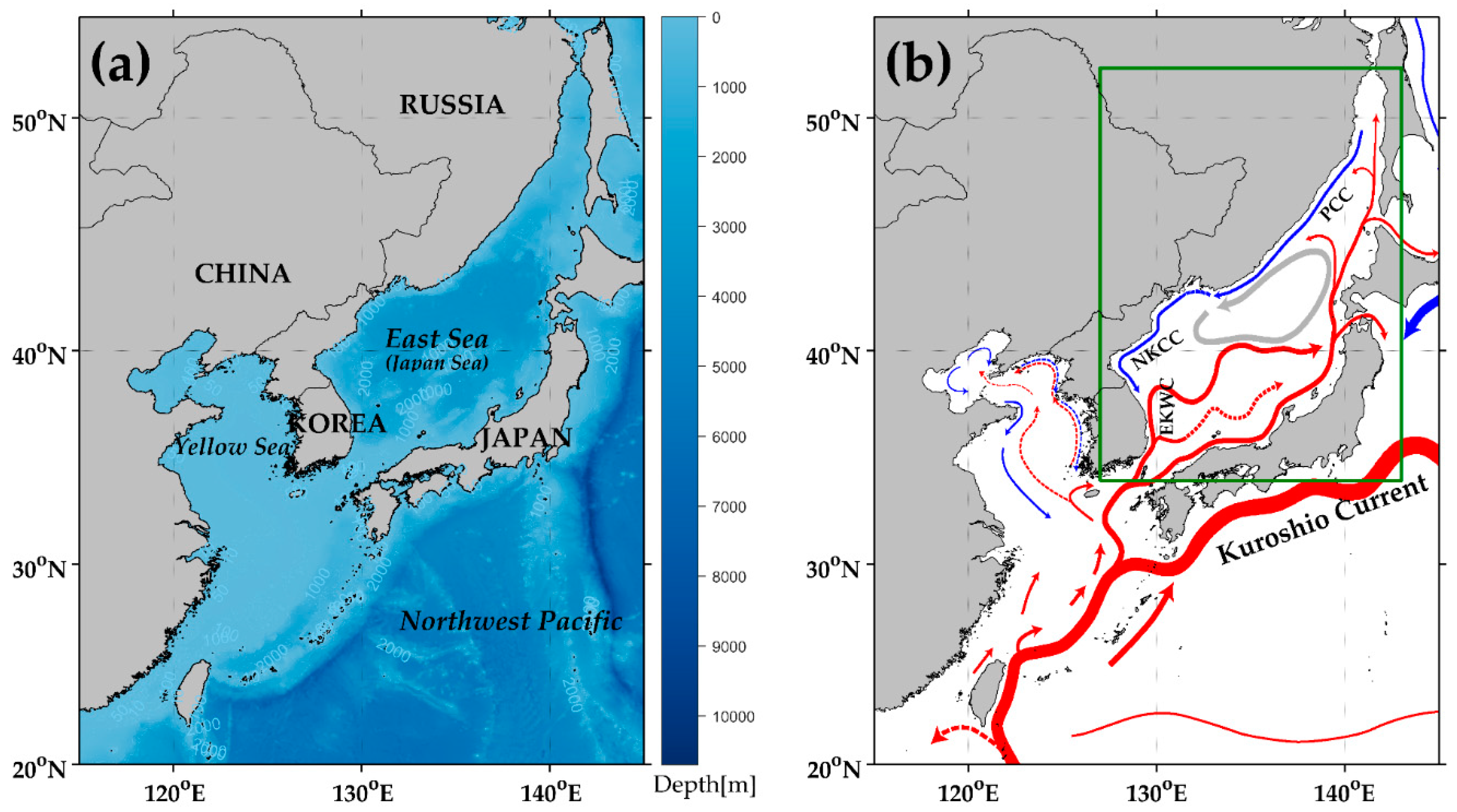
The East Sea (Sea of Japan, EJS) is one of the marginal seas of the Northwest Pacific Ocean, located at the far-eastern end of the Asian continent with the cold and warm current systems (
Figure 1) [
17]. As it is located in the mid-latitude region affected by the Siberian High in winter and by the North Pacific High in summer, it provides a good opportunity for investigating the SST trends in association with changes in the atmospheric conditions over decades. Time series of the SST in the EJS reveal an increasing trend, depending on the period of the data, that is much stronger than that of the global ocean for the observation period from 1982 to 2006 [
11]. Only a few studies have investigated the spatiotemporal pattern of the SST warming trend in the EJS [
18,
19], despite its being an ideal model system for studying the impact of recent regional changes due to change in global ocean warming. Moreover, none of the existing studies have considered the potential effect of the observed increasing tendency toward extremely cold weather in the wintertime using multi-decadal satellite data.
Therefore, in this study, we examined long-term SST trends and recent trend changes in the EJS, which are very important to the climate of the Korean peninsula. The objectives of this study are 1) to estimate the fundamental variations and derive the trend in the long-term SST in the EJS over the 37-year-long observation period, from 1982 to 2018; 2) to investigate any tendency of the SST trends by applying a 20-year-wide sliding window to the total SST database to illustrate a significant increase in the occurrence of SST cooling events in recent decades, and reveal specific seasonal variations in the SST trends focused on the SST cooling; 3) to uncover any relation of the SST trends to extremely hot or cold events; and 4) to examine the relationship between the slowdown of the SST increase rate and the Arctic Oscillation (AO), using the wavelet coherency analysis.
2. Data and Methods
2.1. Satellite Data
Several satellite databases include data on the EJS (e.g., optimum interpolation SST (OISST), multi-scale ultra-high resolution SST (MUR SST), operational SST and sea ice analysis (OSTIA), extended reconstructed SST (ERSST), and Hadley Centre sea ice and SST (HadISST)). These datasets are characterized by various spatial-temporal resolutions and data periods. MUR SST and OSTIA contain data in high temporal resolution (one day) and spatial resolutions of 1 km and 0.05°, respectively. Despite such high spatiotemporal resolutions, these datasets cover relatively short time periods (since May 2002 for the MUR SST database and since April 2006 for the OSTIA database). The other SST databases, such as ERSST and HadISST, cover longer time periods, since 1854 and 1870, respectively. However, their spatial resolutions are relatively low, at 2° and 1°, respectively, and their temporal resolutions are low (one month), which makes it difficult to determine the details of the SST changes in the EJS.
Therefore, in this study, the daily OISST V2 high-resolution data provided by National Oceanic and Atmospheric Administration (NOAA)/Earth System Laboratory (ESRL)/Physical Science Division (PSD), were used to investigate the long-term SST variations in the EJS. This is a global dataset, produced by the optimal interpolation of the advanced very high-resolution radiometer (AVHRR) satellite data with ship and buoy data [
20]. It has a spatial resolution of 0.25° × 0.25°, a time resolution of one day, and has been producing SST data since September 1981. Thus, the present study used the OISST database for the 37-year-long observation time, from 1982 to 2018.
2.2. In-Situ Data
For validating trends in the satellite SST data, in-situ temperature measurements performed by the Korea Oceanographic Data Center (KODC), with a temporal resolution of 2 months, were additionally used when analyzing the southwestern part of the EJS. These data have been acquired by regular stations in an ongoing study that has been initiated by the National Fisheries Research and Development Institute (NFRDI) in 1961. We selected only the 0-m temperature data out of the KODC database, at the standard depths from 0 m to 500 m or deeper depths (e.g., 0, 10, 20, 30, 50, 75, 100, 125, 150, 200, 250, 300, 400, 500 m). The regular measurement stations of the KODC are concentrated in the coastal regions with relatively small numbers of stations in the offshore regions. By contrast, the satellite SST database has a coarse spatial resolution of 0.25° × 0.25°. Owing to the low resolution of the satellite data, we dropped the data from a few stations nearest to the coastal line, for comparison of the SST trends in the offshore regions, by considering the resolution of the satellite data.
2.3. Arctic Oscillation (AO) Index
The AO index data from NOAA/National Centers for Environmental Prediction (NCEP)/Climate Prediction Center (CPC) were used to delineate the potential causes of recent changes attributed to extreme events in the EJS. The AO index pattern was defined as the first leading mode based on the EOF (Empirical Orthogonal Function) analysis of monthly mean height anomalies at 1000 hPa [
21]. As the AO index exhibits high variability during the wintertime, the index mainly reflects the AO characteristics during the wintertime. Although the EJS is located in the mid-latitude region, far from the Arctic region, the atmospheric conditions in the wintertime are quite similar, with very low air temperature and high wind speed over the sea surface, especially in the northern part of the EJS. The AO index is strongly correlated to surface air temperature variations over the Eurasian continent [
21,
22,
23]. Thus, a negative (positive) AO index reflects a higher (lower) Siberian High and a very low (high) surface air temperature over eastern China [
24,
25]. The variability of Aleutian Low also shows a strong relation to the AO index [
26]. Therefore, the relationship between the AO index and SST variability was investigated to explain recent changes in the SST variations.
2.4. Empirical Orthogonal Function (EOF) Analysis
Principal components of variations in time series data can be decomposed using the EOF analysis. The EOF analysis was performed to extract the dominant variability components in the SST data. This method aims at decomposing a data set into a product of a set of spatial patterns and time series [
27,
28,
29], as follows:
where
is the data set,
is the position,
is the time,
is the spatial pattern of the k-th mode,
is the amplitude time series of the k-th mode, and
is the number of spatial elements. The functions
, which are the basis functions, are chosen to be orthogonal to the other basis functions, to account for as much variance as possible, as follows:
where
is the Kronecker delta.
Using this method, it is possible to study spatiotemporal patterns of climate variability. Therefore, since its introduction to geophysics by [
30], this approach has been widely used in meteorology and oceanography (e.g., [
31,
32,
33,
34]).
2.5. Wavelet Coherency Analysis
We applied wavelet coherence analysis to detect variations in coherence and phase difference between two data sets. Wavelet analysis was first applied to each data. Wavelet analysis is one of the tools for analysis of localized power variations within a time series, and has been used in numerous geophysics studies [
35,
36,
37]. By decomposing a time series into the time-frequency space, this analysis allows to determine both the dominant modes of variability and how these modes vary in time. One particular wavelet is defined as [
37]
where
is dimensionless frequency and
is dimensionless time.
Wavelet coherence captures the correlation between two signals in both the time and frequency domains. It is defined as [
38]
where
is a smoothing operator,
is a scale,
is a continuous wavelet transform, and
, where
denotes complex conjugation. Wavelet coherence takes values between 0 (no correlation) and 1 (full correlation).
3. Results
3.1. Spatial and Temporal Variability of SST
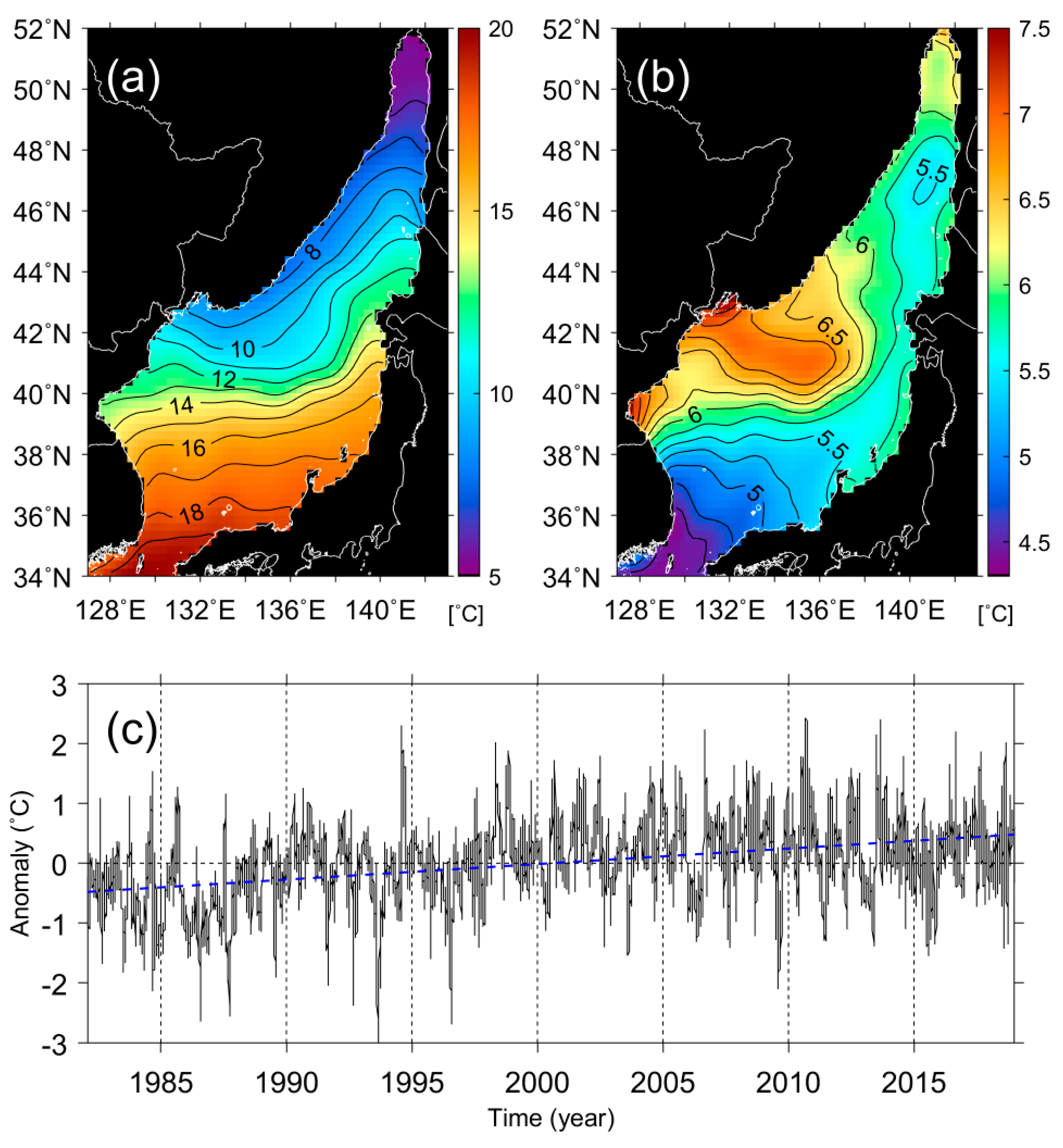
Figure 2 shows the average characteristics of the SST variations in the study area. Going from the southern part of the EJS to its northern part, the mean SST variation decreases from ~20 °C in the Korea Strait to ~5 °C in the Tatar Strait, with relatively concentrated SST differences along the subpolar front (SPF) along the zonal line of about 40°N [
39]. The spatial distribution of the standard deviation of SST variations reveals a striking contrast between the continental side (with high values, above 6 °C) and the offshore Japanese side (with relatively low values, under 6 °C) (
Figure 2b). Especially near Vladivostok (near 132°E and 42°N), large standard deviations (>8 °C) are observed, which implies extreme SST cooling owing to the Siberian outbreak in the wintertime [
40].
In contrast to the time-averaged pattern of the SST, the time series of spatially averaged monthly SST anomalies (SSTAs), from 1982 to 2018, over the entire EJS, exhibits high variability with frequent and random-like peaks, as shown in
Figure 2c. It is noted that the SSTA variation tends to increase during the initial stage of the observation period, from 1982 to mid-1990s. The overall trend in the SSTA amounted to 0.26 °C decade
−1, and was statistically significant within the 95% confidence level, as indicated by the dashed line in
Figure 2c. This warming trend is considered to be relatively strong, compared with that of the global ocean, which was estimated at 0.11 °C decade
−1 based on the observations from 1971 to 2010 [
1].
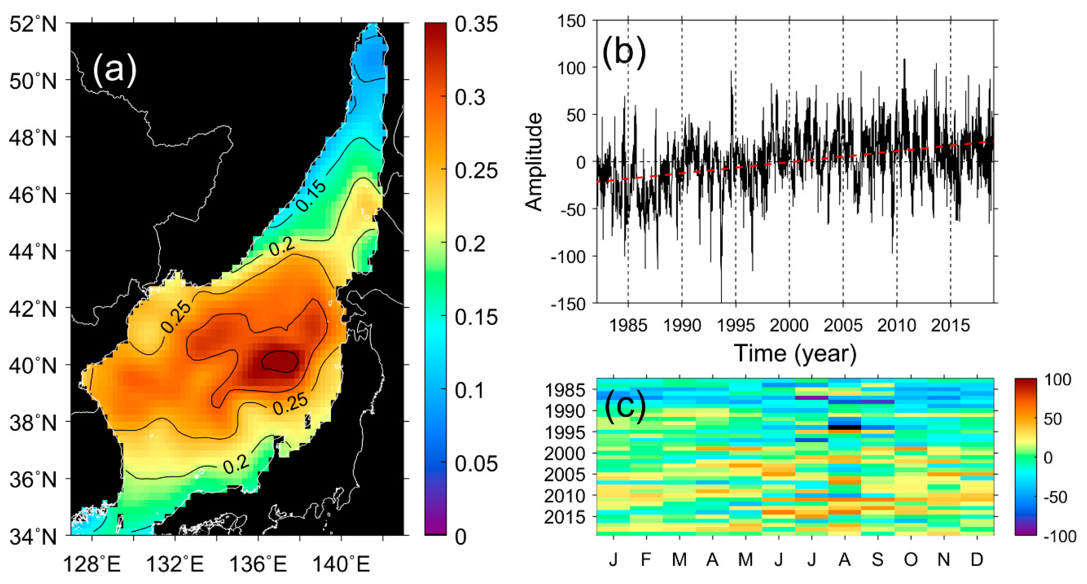
To understand the principal mode of the spatial and temporal variability of the SST, the EOF analysis was performed using the 37-year-long SSTA data. In the first mode (39.02%), the eigenvectors of the SSTA were all positive, implying a characteristic SST warming (
Figure 3). The highest values were observed to the southwest of the Tsugaru Strait (136–139°E and 39–40°N), which was reported from the analysis of in-situ temperature measurements in [
19]. This core corresponds to the region with the highest warming trend, as will be explained later. A slowdown in the increasing tendency of the EOF amplitudes appeared over the recent two decades, from 2000 to 2018, which corresponded to the temporal variations in the SSTA, as shown in
Figure 2c.
3.2. Long-Term Trends of the SST
The slowdown-like feature of the SST warming, suggested by the SSTA variations in
Figure 2c and by the time-varying amplitudes for the first EOF of the SST in
Figure 3b, revealed a steeper trend in the initial observation stage of the observation period and more moderate warming during the recent decades. This raises the question of whether the sea surface has been experiencing warming despite the slowdown with frequently occurring cooling events. To explore the SST warming rate at different spatial locations, the linear tendency in the SST warming was estimated for the entire observation period, from 1982 to 2018 (
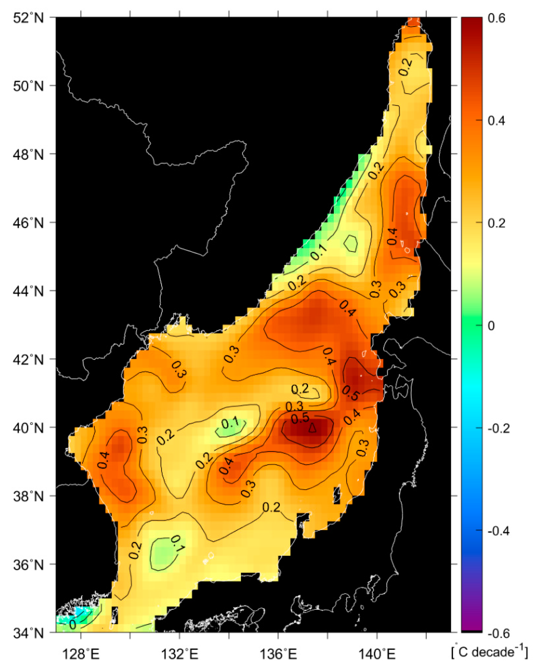
Figure 4). All the SST variations revealed positive trends, ranging up to 0.60 °C decade
−1, with an average of 0.27 °C decade
−1. This indicates that the EJS is still exposed to a warming environment with positive trends. The trend cores, with larger values, appear to be in the central and eastern EJS. The warming trend was the highest in the 136–139°E and 39–40°N regions of the middle eastern part of the EJS. Cores with trends above 0.50 °C decade
−1 were observed in the west of Tsugaru Strait (~41°N) and cores with trends above 0.40 °C decade
−1 were observed in the west of Soya Strait (~46°N). Other cores with trends above 0.40 °C decade
−1 appeared even near Wonsan Bay (~39°N). Although there are some differences between regions in terms of the warming rate, all the analyzed EJS regions revealed positive trends (
Figure 4).
Regarding the regions with low SST warming trends, below 0.10 °C decade
−1, there were some specific regions with very weak warming; for example, the region around 40°N and 133–135°E, along the Russian coast off the Primorye, or the southwestern portion of the EJS (36–37°N and 131–132°E). As evidenced in
Figure 4, most of the EJS have been experiencing severe SST warming over almost four decades. In contrast to the general trends in most of the EJS, why do some regions have such weak warming trends? We posited that different regions must have been exposed to different atmospheric environments or different oceanic environments over decades. To be able to understand the processes responsible for the appearance of such weakly-warming sites, it is necessary to validate the SST warming rates. Thus, we estimated the warming rates using long-term in-situ measurements from the coastal region around the Korean peninsula; the results of this estimation are presented in the following section.
3.3. Comparison of the SST Trends to In-Situ Measurements
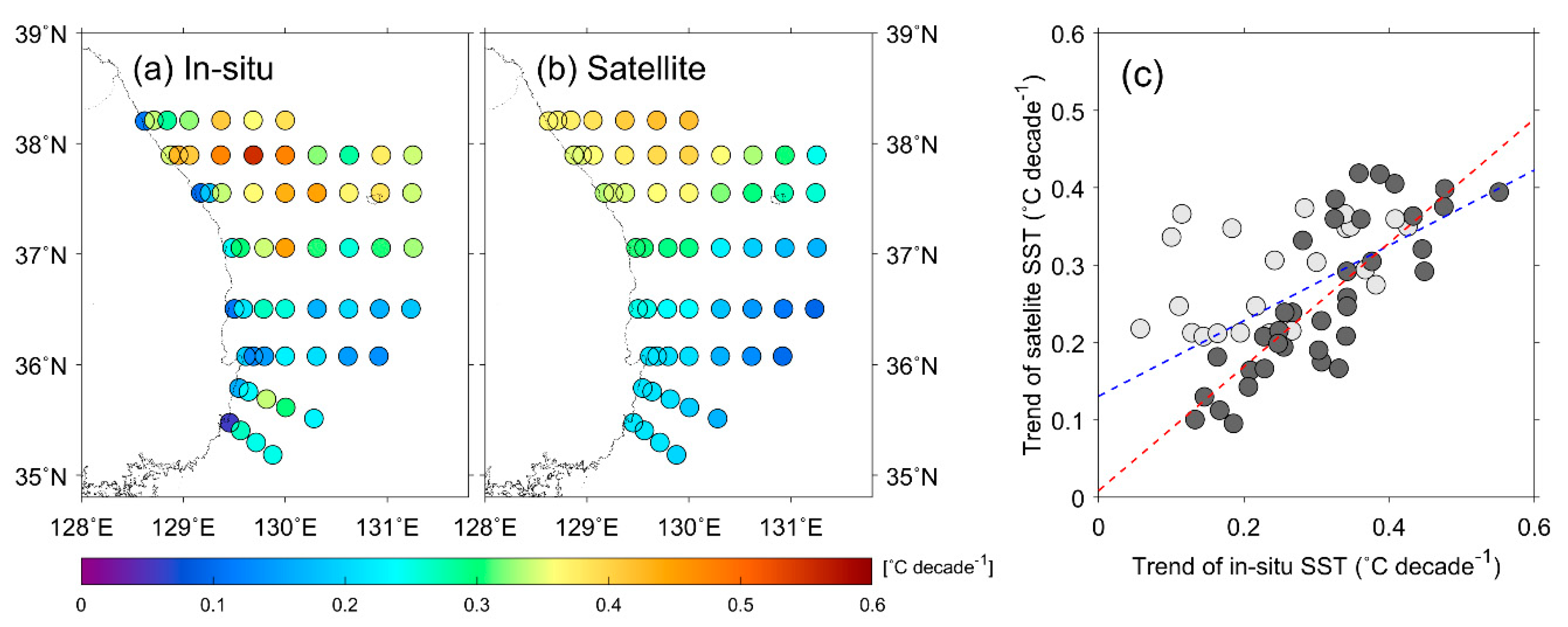
Using long-term temperature measurements from the KODC database, the trends of the surface temperatures at each station were estimated as shown in
Figure 5a. The circles in
Figure 5a denote the locations of the KODC regular observation stations, based on bimonthly observations at 79 stations in the EJS, to measure the water temperature and salinity in the southwestern portion of the EJS. The in-situ measured temperatures exhibited positive correlation with surface warming, with 95%-confidence level, regardless of coastal or offshore regions, which implied a general tendency of surface warming. One interesting observation is that the stations north of 37°N reported much higher warning rates (>0.40 °C decade
−1) than the stations located to the south (<0.20 °C decade
−1).
The satellite SST database used in this study has a spatial resolution of 0.25° × 0.25°, which is different from the point measurements of the KODC data. Due to the differences of data samplings, such as spatial differences and observational times, it is expected that the satellite SSTs might produce non-negligible differences of the trends with in-situ measurements. In spite of such differences, satellite-based SST warming rates in
Figure 5b were in a good agreement with the in-situ SST trends in terms of the overall distribution of the trends, with relatively higher warming and weaker warming in the southern region. When comparing all data between the trends of in-situ SST and satellite SST, the obtained slope was 0.49 (R
2 = 0.36) and the correlation coefficient was 0.60 (p = 6.13E–7) (
Figure 5c). The satellite data used in this study have a relatively large spatial grid of ~0.25°, and those data included microwave SSTs owing to a higher probability of clouds in the coastal regions, with frequent variations of air temperature and moisture conditions. When all of the points, including both close (bright gray) and far (dark gray) points from the coastline, were considered, the satellite-based and in-situ based SST trends were in general concordance, but had a relatively weak correlation and high scatter in the weak-trend range of in-situ temperatures. By contrast, the KODC trends without the points near the coastal regions within 0.25° from the coastline revealed a good correlation between the two trends, as illustrated by the red dashed line in
Figure 5c. An improved comparison result was obtained for the offshore regions; the obtained slope was 0.80 (R
2 = 0.67) and the correlation coefficient was 0.82 (p = 1.22E–9). All of these results support the hypothesis that the retrieved SST data from the satellite data, once those too close to the coast are excluded, can be used for the analysis of oceanic surface warming.
3.4. Moving Trends in the SST
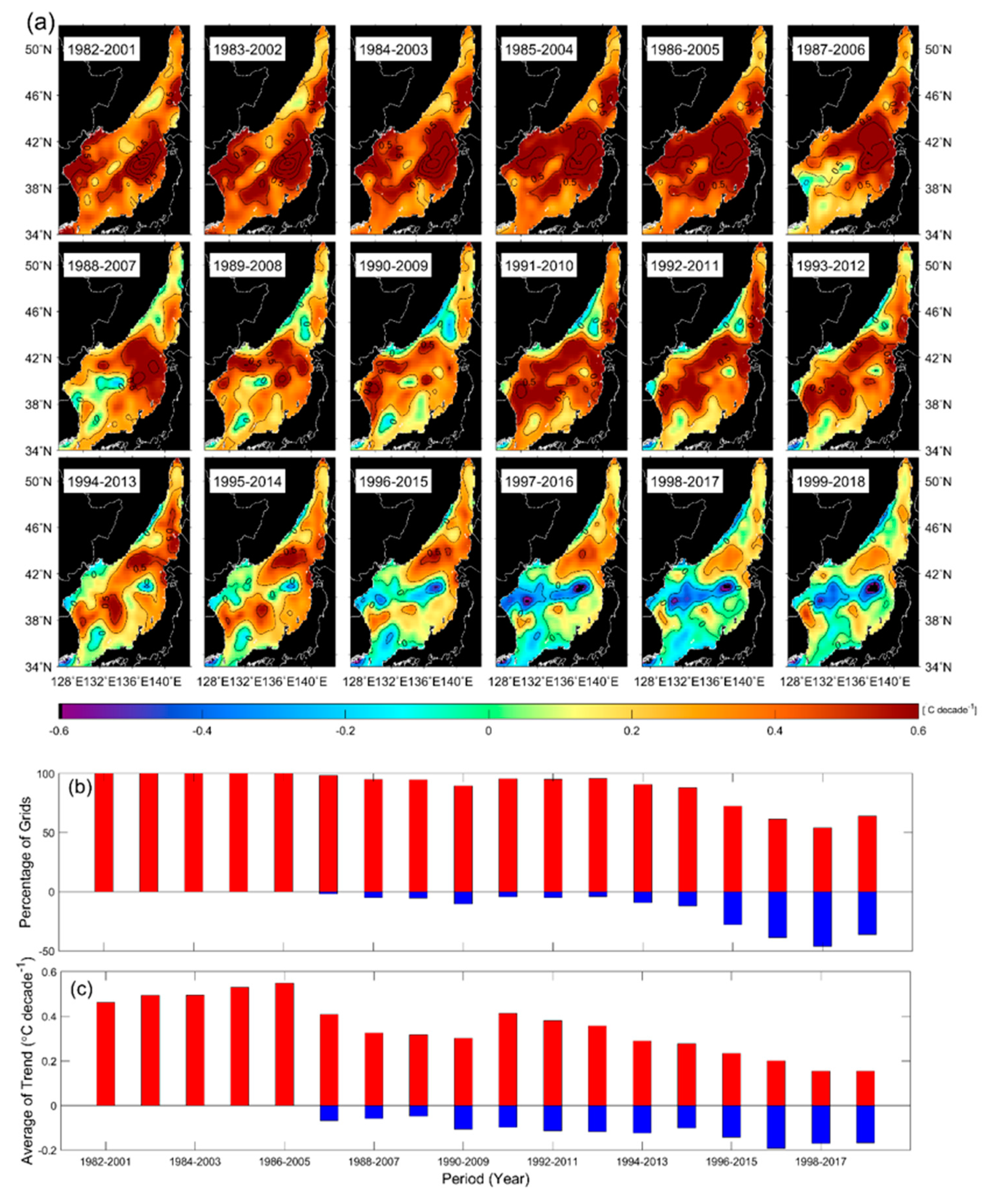
As demonstrated by the analysis of long-term variations of the SSTA and the time-varying amplitude of the first EOF mode of the SSTA (
Figure 2 and
Figure 3b), the slopes for those features that showed increasing trends exhibited slow-time-scale variations with relatively rapid warming during the initial observation period decades, while milder warming was observed during recent decades. To analyze the temporal variability in the warming trends, we calculated the multi-year moving trends in the SST by applying a 20-year-wide temporal domain for the estimation of linear trends, for all spatial grids. The 20-year period was determined by considering relatively high interannual variability of SSTs in the EJS at dominant frequency amounting to 7 years according to the previous study [
41].
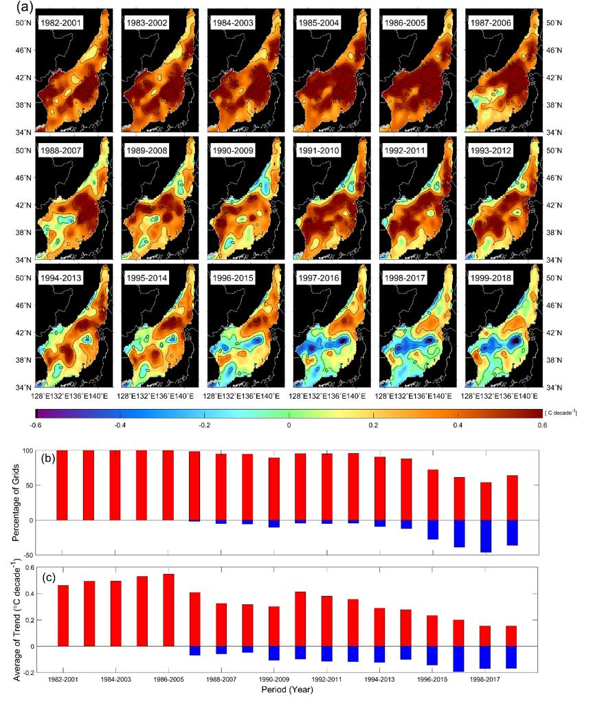
Figure 6a shows the time series of the spatial distribution for the 20-year-long moving trends in the SST variations, during the observation period from 1982 to 2018. The first image shows the SST warming rates over the entire region for the first 20 years of observation, from 1982 to 2001. The warming trends increased continuously, until the period from 1986 to 2005; however, they began to reduce gradually and even switched to cooling from the SPF region, for the observation period from 1987 to 2006. Especially, they seemed to have been strongly reducing along the Russian coast, for the observation period from 1988 to 2007. One notable feature of that trend is that a negative trend, that is SST cooling, appeared along the SPF in the central portion of the EJS, as can be clearly seen for the observation period from 1996 to 2015, as well as for the following observation period.
To examine such slowdown features in the SST warming trends in more detail, the time series of the areal percentages of the positive (red) and negative (blue) trends for each period are shown in
Figure 6b. For the initial observation periods, from 1982 to 2001 and from 1986 to 2005, all of the EJS regions exhibited a positive warming tendency by occupying 100% of the positive trend without any regions with negative trends. However, for the observation period from 1987 to 2006, negative mean trends began to appear at a rate of 1.80% of the total number of grids. The number of the grids corresponding to the SST cooling, as marked by blue bars in
Figure 6b, increased exponentially with a wide spreading of the surface cooling with time. This tendency began to appear for the observation period from 1987 to 2006 and have been intensifying until the recent two decades.
The averaged trends in the SST warming and cooling exhibited gradual variations over time (
Figure 6c). The trend reached a maximum of ~0.55 °C decade
−1 for the period of 1986–2005 and continuously decreased to 0.15 °C decade
−1 during the recent two decades. As can be seen in the last three bars for the observation period from 1997 to 2016, the mean rate of the SST cooling (–0.19, –0.17, and –0.17 °C decade
−1, respectively) amounted to a similar trend of the SST warming (0.20, 0.15, and 0.15 °C decade
−1, respectively), in spite of the widespread region for an overall observed SST warming. In other words, the number of the grids with the SST cooling tendency gradually increased while that with the SST warming tendency reversely decreased with time. This implies that the SST cooling events have been more intensively increasing in relatively small regions concentrated in the frontal zones in the central part of the EJS.
3.5. Monthly Variations in the SST Trends
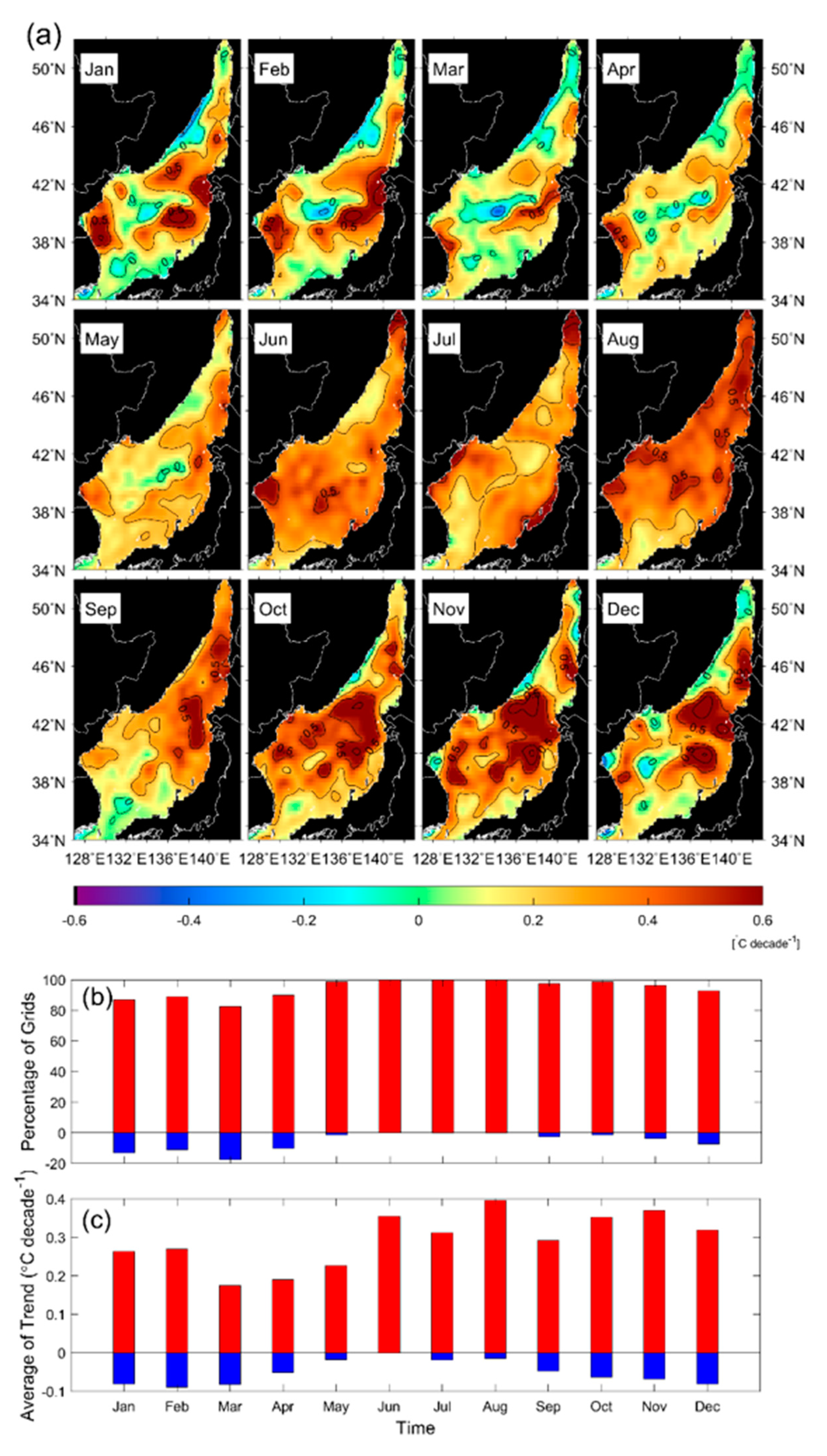
As mentioned earlier, the degree of the SST warming of the EJS has been mitigated over recent decades. It is important to investigate any potential seasonal impact on the observed reduction in the increase of the warming rate. Thus, we calculated the monthly SST trends, their areal fractions, and the average trend values, for both warming and cooling separately (
Figure 7). The monthly trends for the summer season, from June to August, appeared to show positive trends over the entire EJS (
Figure 7a). However, the other months, except for the summer months, revealed the existence of weak negative trends along the Russian coast, the SPFs, and the southwestern part of the EJS near the Korea Strait.
Especially in the springtime (during the March–May period), negative trends were concentrated along the SPF region in the central part of the EJS. By contrast, strongest warmings appeared from June to November, and extended to the eastern part of the EJS. In the wintertime (during the December–February period), the pattern of monthly SST trends was similar to that for the total trend in
Figure 4. In other words, the warming trend was large for all seasons except for spring, and especially so from August to November. This observation was quite different from previously reported warming that has been attributed to the increasing role of wintertime SST variations [
17].
The areal coverage of cooling constituted a relatively high fraction, from 7% in December to the maximum of 18% in March (
Figure 7b) in winter and spring. The strongest warming trend of ~0.40 °C decade
−1 appeared in August, while the weakest warming trend, ~0.18 °C decade
−1, appeared in March (
Figure 7c). Concerning the cooling, the strongest cooling trend was about –0.09 °C decade
−1, and was observed for February and March.
3.6. Occurrence of Extremely High/Low SSTs
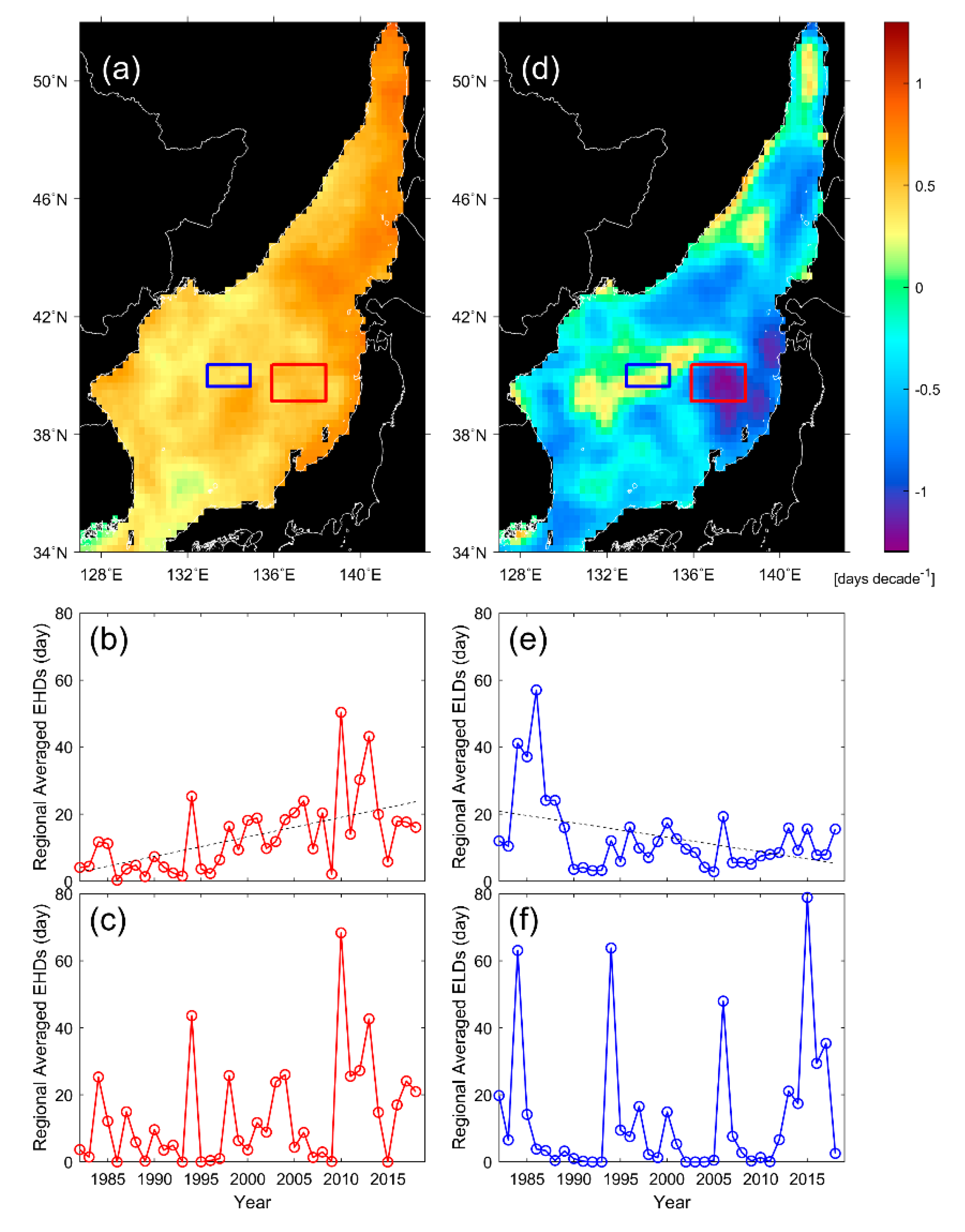
We analyzed the occurrence of extreme SST events for determining the potential causes of the observed weakening of the warming trend and the seasonal shift of the warming trend leading from winter to summer. Before defining extreme events, daily SSTAs were calculated by subtracting the climatological mean from the SST values for the same date. Extremely high SST days (EHDs) were defined as days within the top 10% (90th percentile) of anomalies in the summertime (June–September). In a similar way, extremely low SST days (ELDs) were defined as days in the bottom 10% of anomalies, but for the wintertime (December–March).
Figure 8a shows the spatial distribution of the trends of the EHD occurrence frequency for the entire observation period of 37 years. It is notable that all regions exhibit positive trends, implying continuous warming of the EJS over the past decades. The spatially averaged value of the EHD occurrence frequency tended to increase with time at a rate of 5.82 days decade
−1 (
Figure 8b). Regarding the cooling events, the spatial distribution of the trends of the ELD occurrence frequency exhibited negative trends for most of the regions in the EJS except for a few regions associated with SPFs, with weakly positive trends of ~0.25 days decade
−1 (
Figure 8d). The time series of the ELDs exhibit the decreasing tendency (–4.31 days decade
−1) with high peaks of ~57 days in the 1980s and minor days of less than 20 days during other periods (
Figure 8e). This overall characteristic is consistent with the long-term warming trend in the EJS.
To understand the difference between cooling and warming regions in the SST variations, we selected two representative regions, marked by blue (weak warming) and red (strong warming) boxes in
Figure 8a,d. As the trend in the strong-warming sites corresponds to the overall warming trend, we focused on the trend in the weak-warming sites.
Figure 8c shows the time series of the EHDs in small regions that exhibited warming trends, revealing the tendency of the EHDs to increase temperature with time, with the highest peak occurring in 2010. However, the trend of the occurrence frequency of the ELDs differed from that of the entire EJS. The high frequency (more than 45 days) of the ELDs seemed to occur somewhat periodically every decade (
Figure 8f). Except for the extremely cold days, most of the ELDs were relatively small, lasting less than 20 days. The occurrence of the ELDs was the highest in 2015 instead of the extremely cold days prior to substantial global warming decades ago. This feature exemplifies the significant role of extremely cold days on the slowdown of the recent SST increase.
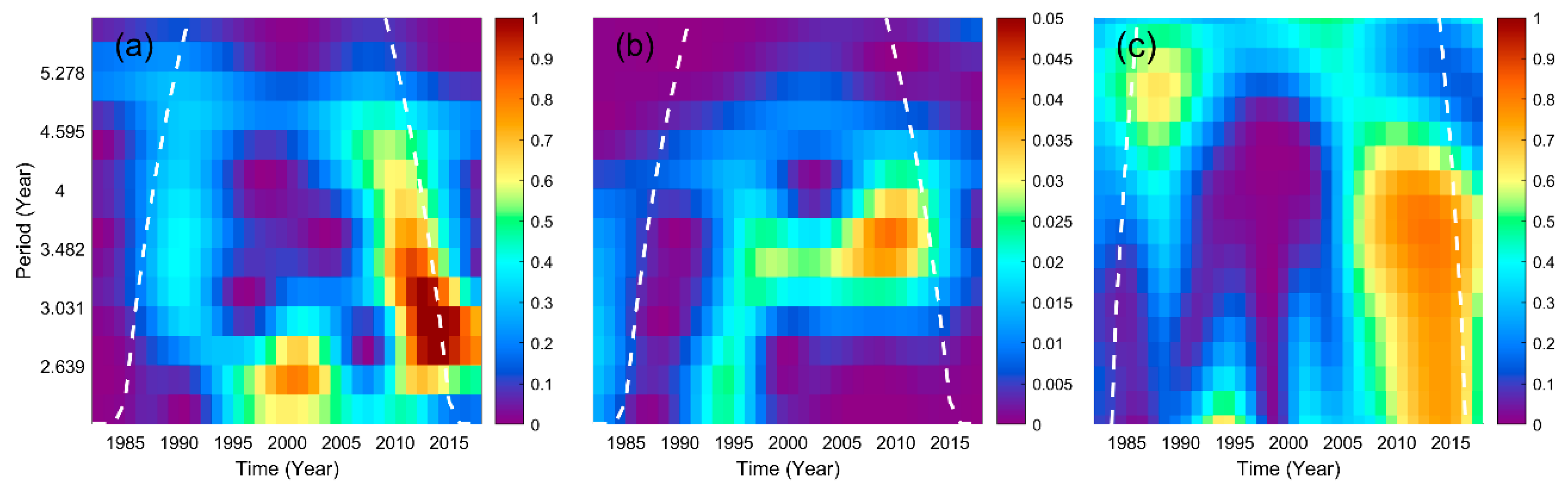
3.7. Relation to the AO
What causes the observed periodic appearance of extremely low SST events? One representatively influential climate index that captures SST variations in the EJS is the AO index. We studied the variability of AO, which, as we posited, could affect the SST in winter in the EJS, especially with respect to extreme events. Thus, we sought to determine if there was significant change in the energy of AO variations with time by performing wavelet analysis of available data; the results of this analysis are shown in
Figure 9a. When considering time periods longer than 3 years, the AO index exhibited relatively low variability in the earlier decades of the observation period. However, higher variability with strong energy variations appeared in the recent decades of the observation period, as shown in
Figure 9a. The results of the wavelet analysis of the AO for wintertime data revealed a large variability with 2–2.5 year-long cycles around the year 2000, and with 2.5–3.5 year-long cycles after 2010 (
Figure 9a). This suggests that the higher variability of changes in the atmospheric and oceanic features in the Arctic Ocean may be related to the recent fast warming and melting of the sea ice [
42,
43,
44]. Next, we asked whether this AO variability can affect the SST trends in the EJS, which is one of the marginal seas of the Northwest Pacific in the mid-latitude region. To answer this question, we performed wavelet analysis of SST variations in the ELDs, and the results of this analysis are shown in
Figure 9b. The highest variability in the SSTA was observed in 2010, with a temporal period of ~3.5 years.
Wavelet coherence was computed for examining a possible relationship between the AO and SSTA in the ELDs. As wavelet coherence quantifies correlation, the coherence takes on the value of 1 if the two analyzed signals are highly correlated.
Figure 9c shows that the coherence between the two signals is above 0.7 (corresponding 95% of confidence level), for the observation period from 2010 to the present time. This suggests that the AO index captures the SST changes and the ELDs during recent decades, and in particular after 2005. One interesting observation is that the coherence between the AO and the SSTA in the ELDs in the EJS exhibited insignificant correlation (below 0.1) for the observation period from 1982 to 2005, over most of the temporal periods. Arctic variations are not expected to affect the SST warming or cooling in the EJS. This implies that the EJS has long been protected from the extreme cold condition of the Arctic region. Thus, changes in the SST warming of the EJS, as shown in
Figure 6, especially the observed slowdown of warming with frequent and random extremely cold days in winter, may have been induced by changes in the AO that occur as a part of the global warming trend.
4. Discussion
According to [
45], who analyzed seasonal trends in the global temperature for the period from 1979 to 2010, the SST in the Northern Hemisphere exhibited a significant warming trend for all seasons in the past decades. At that time, the warming rate was reported to be larger in autumn and winter than in spring and summer. A similar result for the SST warming of the EJS was reported, stating that the warming was more significant in the wintertime than in the summertime for the period from 1891 to 2005 [
18]. As one of the effects of global climate change on changes in the SST variation in local regions, [
11] showed that the SST in the EJS exhibited an overall increase of more than 0.9 °C over the time period of 25 years, from 1982 to 2006, including a rapid increase (more than 12-fold) in the global warming rate at 1.67 °C decade
−1 during the observation period from 1986 to 1998.
In contrast to the previous studies of the warming of the EJS, this study demonstrated a reverse tendency that the higher SST warming have been led by change in summertime SSTs rather than that in winter by accompanying with the reduction of warming rates regardless of season. Nevertheless, the overall warming rates were still positive, not only over the entire period, but also in the recent decades. In particular, SST cooling at specific regions of the EJS, such as in the central region of the SPFs and along the Russian Primorye coast, has begun to appear for the recent decades after 2003. Such a cooling trend appeared in all seasons except for the summer. This suggests that winter, which led to a warming trend previously, may contribute to the frequent increase of ELDs as a measure of surface cooling in the last years.
What are the main causes of the monthly distinction of SST cooling rates? What causes the slowdown of general SST warming in the EJS? What is the role of change in SST in winter on the weakening of SST warming? It is known that the Arctic warming is much stronger than changes in lower latitudes [
42,
44]. It was reported that such Arctic warming can influence the occurrence of extreme atmospheric weather in the mid-latitudes through dynamical pathways such as changes in the storm tracks, the jet stream and the planetary waves [
46]. In addition, [
47] argued that severe winters may occur in the mid-latitude regions due to the northerly flow of cold air in the atmosphere, resulting from the Arctic warming accompanied by the local development of an anomalous anticyclone and the downstream development of the mid-latitude trough. Such atmospheric cooling of mid-latitude regions induced by the Arctic warming is expected to produce SST cooling during winter outbreaks over the sea surface of the EJS. This argument supports the results of this study concerning the less warming and re-initiation of surface cooling in the recent decades. This corresponds to recent finding on the re-initiation of bottom water formation in the EJS sensitive to changing surface conditions and atmospheric forcing [
48].
The findings of the present study could be attributed to the regional-scale imprints of the large-scale global warming hiatus (GWH) that is referred to as the global warming slowdown, on a period of relatively small warming in the surface temperature of the Earth [
12,
13]. Additionally, it is suggested that the Antarctic Oscillation (AAO), also known as the Southern Annular Mode (SAM), which is a low-frequency mode of atmospheric variability of the Southern Hemisphere, can affect not only the climate change in the Southern Hemisphere but also in the Northern Hemisphere [
49,
50,
51]. The AAO is capable of influencing the AO through remotely connected atmospheric variability. This study demonstrates one of the examples of the impact of Artic environmental changes and GWH on the regional SST variations, and discusses the characteristics and causes of the regional SST variations in the EJS. Therefore, it is expected that this study could be further explored for a deep understanding of the linkage between regional responses and other climate indices.
5. Conclusions
The present study showed long-term SST warming trends in almost all of the EJS regions, during the 37-year-long observation period, from 1982 to 2018. The trend was related to the slowdown of the SST warming, especially in the SPF area. Analyzing the changes in the extremely high SST events in the summertime and extremely low SST events in the wintertime, regional averages for the EJS exhibited a reduction in the ELD and an increase in the EHD, consistent with the overall warming trend. However, in the areas where warming was relatively weak, the ELD exhibited large values frequently, with the maximal value observed within the last 5 years. As a result of examining the relationship between the AO and the SSTA corresponding to the ELD, the consistency between these two variables increased, especially for the recent decade. This suggests that changes that take place in the Arctic Ocean can explain some recent SST changes in the EJS through changes in atmospheric effects.
The SST warming and cooling, presented in this study, corroborate an oceanic response of the EJS through the atmospheric connection between the extremely cold Arctic environment and mid-latitude regions. This implies that the EJS, as a small-scale replica of the global ocean, is exposed to the overall global warming trend as well as to the extreme surface cooling that originates in the Arctic Ocean. This suggests that the EJS, as one of the marginal mid-latitude seas, might be strongly linked with the polar region in winter, in spite of the distance. Thus, further analysis is needed for an in-depth understanding of long-term SST changes in the EJS in the warming climate.
Author Contributions
Conceptualization, K.-A.P.; data curation, E.-Y.L.; methodology, K.-A.P. and E.-Y.L.; writing –original draft preparation, E.-Y.L.; writing – review and editing; K.-A.P. and E.-Y.L.
Funding
This work was funded by the Korea Meteorological Administration Research and Development Program under Grant KMI2018-05110.
Acknowledgments
We thank anonymous reviewers for their insightful comments, which helped to make an improvement to this manuscript. NOAA OISST V2 data provided by the NOAA/OAR/ESRL PSD, Boulder, Colorado, USA, from their Web site at
https://www.esrl.noaa.gov/psd.
Conflicts of Interest
The authors declare no conflicts of interest.
Abbreviations
The following abbreviations are used in this manuscript:
| AO | Arctic Oscillation |
| AAO | Antarctic Oscillation |
| AVHRR | advanced very high resolution radiometer |
| EJS | East Sea (Sea of Japan) |
| EKWC | East Korea Warm Current |
| ELD | extremely low SST day |
| EHD | extremely high SST day |
| EOF | empirical orthogonal function |
| ERSST | extended reconstructed SST |
| GWH | global warming hiatus |
| HadISST | Hadley Centre sea ice and SST |
| KODC | Korea Oceanographic Data Center |
| MUR SST | multi-scale ultra-high resolution SST |
| NFRDI | National Fisheries Research and Development Institute |
| NKCC | North Korea Cold Current |
| NOAA | National Oceanic and Atmospheric Administration |
| OISST | optimum interpolation SST |
| OSTIA | operational SST and sea ice analysis |
| PCC | Primorye Cold Current |
| SPF | subpolar front |
| SST | sea surface temperature |
| SSTA | SST anomaly |
References
- IPCC. Climate Change 2014: Synthesis Report. Contribution of Working Group I, II and III to the Fifth Assessment Report of the Intergovernmental Panel on Climate Change; Core Writing Team, Pachauri, R.K., Meyer, L.A., Eds.; IPCC: Geneva, Switzerland, 2014; p. 151. [Google Scholar]
- Domingues, C.M.; Church, J.A.; White, N.J.; Gleckler, P.J.; Wijffels, S.E.; Barker, P.M.; Dunn, J.R. Improved estimates of upper-ocean warming and multi-decadal sea-level rise. Nature 2008, 453, 1090–1093. [Google Scholar] [CrossRef]
- Lyman, J.M.; Johnson, G.C. Estimating annual global upper-ocean heat content anomalies despite irregular in-situ ocean sampling. J. Clim. 2008, 21, 5629–5641. [Google Scholar] [CrossRef]
- Liu, L.; Lozano, C.; Iredell, D. Time–Space SST Variability in the Atlantic during 2013: Seasonal Cycle. J. Atmos. Oceanic Technol. 2015, 32, 1689–1705. [Google Scholar] [CrossRef]
- Gentemann, C.L.; Fewings, M.R.; García-Reyes, M. Satellite sea surface temperatures along the West Coast of the United States during the 2014–2016 northeast Pacific marine heat wave. Geophys. Res. Lett. 2017, 44, 312–319. [Google Scholar] [CrossRef]
- Levitus, S.; Antonov, J.I.; Wang, J.; Delworth, T.L.; Dixon, K.W.; Broccoli, A.J. Anthropogenic warming of Earth’s climate system. Science 2001, 92, 267–270. [Google Scholar] [CrossRef] [PubMed]
- Barnett, T.P.; Pierce, D.W.; Schnur, R. Detection of anthropogenic climate change in the world’s oceans. Science 2001, 292, 270–274. [Google Scholar] [CrossRef] [PubMed]
- Pierce, D.W.; Barnett, T.P.; AchutaRao, K.M.; Gleckler, P.J.; Gregory, J.M.; Washington, W.M. Anthropogenic warming of the oceans: Observations and model results. J. Clim. 2006, 19, 1873–1900. [Google Scholar] [CrossRef]
- Levitus, S.; Antonov, J.I.; Boyer, T.P.; Stephens, C. Warming of the world ocean. Science 2000, 287, 2225–2229. [Google Scholar] [CrossRef]
- Barnett, T.P.; Pierce, D.W.; AchutaRao, K.M.; Gleckler, P.J.; Santer, B.D.; Gregory, J.M.; Washington, W.M. Penetration of human-induced warming into the world’s oceans. Science 2005, 309, 284–287. [Google Scholar] [CrossRef]
- Belkin, I.M. Rapid warming of large marine ecosystems. Prog. Oceanogr. 2009, 81, 207–213. [Google Scholar] [CrossRef]
- Easterling, D.R.; Wehner, M.F. Is the climate warming or cooling? Geophys. Res. Lett. 2009, 36, L08706. [Google Scholar] [CrossRef]
- Meehl, G.A.; Teng, H.; Arblaster, J.M. Climate model simulations of the observed early-2000s hiatus of global warming. Nat. Clim. Change 2014, 4, 898. [Google Scholar] [CrossRef]
- Seneviratne, S.I.; Donat, M.G.; Mueller, B.; Alexander, L.V. No pause in the increase of hot temperature extremes. Nat. Clim. Change 2014, 4, 161. [Google Scholar] [CrossRef]
- Johnson, N.C.; Xie, S.P.; Kosaka, Y.; Li, X. Increasing occurrence of cold and warm extremes during the recent global warming slowdown. Nat. Commun. 2018, 9, 1724. [Google Scholar] [CrossRef] [PubMed]
- Wang, Q.; Li, Y.; Li, Q.; Liu, Y.; Wang, Y.N. Changes in means and extreme events of sea surface temperature in the east china seas based on satellite data from 1982 to 2017. Atmosphere 2019, 10, 140. [Google Scholar] [CrossRef]
- Park, K.A.; Park, J.E.; Choi, B.J.; Byun, D.S.; Lee, E.I. An oceanic current map of the East Sea for science textbooks based on scientific knowledge acquired from oceanic measurements. Sea 2013, 18, 234–265. [Google Scholar] [CrossRef]
- Yeh, S.W.; Park, Y.G.; Min, H.; Kim, C.H.; Lee, J.H. Analysis of characteristics in the sea surface temperature variability in the East/Japan Sea. Prog. Oceanogr. 2010, 85, 213–223. [Google Scholar] [CrossRef]
- Na, H.; Kim, K.Y.; Chang, K.I.; Park, J.J.; Kim, K.; Minobe, S. Decadal variability of the upper ocean heat content in the East/Japan Sea and its possible relationship to northwestern Pacific variability. J. Geophys. Res. Oceans 2012, 117, C02017. [Google Scholar] [CrossRef]
- Reynolds, R.W.; Smith, T.M.; Liu, C.; Chelton, D.B.; Casey, K.S.; Schlax, M.G. Daily high-resolution-blended analyses for sea surface temperature. J. Clim. 2007, 20, 5473–5496. [Google Scholar] [CrossRef]
- Thompson, D.W.J.; Wallace, J.M. The Arctic Oscillation signature in the winter geopotential height and temperature fields. Geophys. Res. Lett. 1998, 25, 1297–1300. [Google Scholar] [CrossRef]
- Thompson, D.W.J.; Wallace, J.M. Annular modes in the extratropical circulation. Part I: Month-to-month variability. J. Clim. 2000, 13, 1000–1016. [Google Scholar] [CrossRef]
- Kerr, R.A. New force in high-latitude climate. Science 1999, 284, 241–242. [Google Scholar] [CrossRef]
- Gong, D.Y.; Wang, S.W.; Zhu, J.H. East Asian winter monsoon and Arctic oscillation. Geophys. Res. Lett. 2001, 28, 2073–2076. [Google Scholar] [CrossRef]
- Isobe, A.; Beardsley, R.C. Atmosphere and marginal-sea interaction leading to an interannual variation in cold-air outbreak activity over the Japan Sea. J. Clim. 2007, 20, 5707–5714. [Google Scholar] [CrossRef]
- Overland, J.E.; Adams, J.M.; Bond, N.A. Decadal variability of the Aleutian low and its relation to high-latitude circulation. J. Clim. 1999, 12, 1542–1548. [Google Scholar] [CrossRef]
- Lagerloaf, G.S.E.; Bernstein, R.L. Empirical orthogonal function analysis of advanced very high resolution radiometer surface temperature patterns in Santa Barbara Channel. J. Geophys. Res. 1988, 93, 6863–6873. [Google Scholar] [CrossRef]
- Kelly, K.A. Comment on ‘EOF analysis of advanced very high resolution radiometer surface temperature patterns in Santa Barbara Channel’ by Gary, S.E. Lagerloef and Robert, L. Bernstein. J. Geophys. Res. 1988, 93, 15753–15754. [Google Scholar] [CrossRef]
- Emery, W.J.; Thomson, R.E. Data Analysis Methods in Physical Oceanography, 1st ed.; Pergamon Press: Oxford, UK, 1998; p. 634. [Google Scholar]
- Lorenz, E.N. Empirical Orthogonal Functions and Statistical Weather Prediction; Massachusetts Institute of Technology: Cambridge, MA, USA, 1956; p. 49. [Google Scholar]
- Craddock, J.M.; Flood, C.R. Eigenvectors for representing the 500 mb geopotential surface over the Northern Hemisphere. Q. J. R. Meteorolog. Soc. 1969, 95, 576–593. [Google Scholar] [CrossRef]
- Kidson, J.W. Eigenvector analysis of monthly mean surface data. Mon. Weather Rev. 1975, 103, 177–186. [Google Scholar] [CrossRef]
- Trenberth, K.E. A quasi-biennial standing wave in the Southern Hemisphere and interrelations with sea surface temperature. Q. J. R. Meteorolog. Soc. 1975, 101, 55–74. [Google Scholar] [CrossRef]
- Weare, B.C.; Navato, A.R.; Newell, R.E. Empirical orthogonal analysis of Pacific sea surface temperatures. J. Phys. Oceanogr. 1976, 6, 671–678. [Google Scholar] [CrossRef]
- Daubechies, I. Ten Lectures on Wavelets; Society for Industrial and Applied Mathematics: Philadelphia, PA, USA, 1992; p. 357. [Google Scholar]
- Foufoula-Georgiou, E.; Kumar, P. Wavelets in Geophysics; Academic Press: Cambridge, MA, USA, 1995; p. 373. [Google Scholar]
- Torrence, C.; Compo, G.P. A practical guide to wavelet analysis. Bull. Am. Meteorol. Soc. 1998, 79, 61–78. [Google Scholar] [CrossRef]
- Torrence, C.; Webster, P. Interdecadal changes in the ENSO-Monsoon system. J. Clim. 1999, 12, 2679–2690. [Google Scholar] [CrossRef]
- Park, K.A.; Ullman, D.S.; Kim, K.; Chung, J.Y.; Kim, K.R. Spatial and temporal variability of satellite-observed subpolar front in the East/Japan Sea. Deep Sea Res. Part. I 2007, 54, 453–470. [Google Scholar] [CrossRef]
- Park, K.A.; Chung, J.Y.; Kim, K.; Cornillon, P.C. Wind and bathymetric forcing of the annual sea surface temperature signal in the East (Japan) Sea. Geophys. Res. Lett. 2005, 32, L05610. [Google Scholar] [CrossRef]
- Park, S.; Chu, P.C. Interannual SST variability in the Japan/East Sea and relationship with environmental variables. J. Oceanogr. 2006, 62, 115–132. [Google Scholar] [CrossRef]
- Serreze, M.C.; Barrett, A.P.; Stroeve, J.C.; Kindig, D.N.; Holland, M.M. The emergence of surface-based Arctic amplification. Cryosphere 2009, 3, 11–19. [Google Scholar] [CrossRef] [Green Version]
- Serreze, M.C.; Barry, R.G. Processes and impacts of Arctic amplification: A research synthesis. Global Planet. Change 2011, 77, 85–96. [Google Scholar] [CrossRef]
- Screen, J.A.; Simmonds, I. The central role of diminishing sea ice in recent arctic temperature amplification. Nature 2010, 464, 1334. [Google Scholar] [CrossRef]
- Cohen, J.L.; Furtado, J.C.; Barlow, M.; Alexeev, V.A.; Cherry, J.E. Asymmetric seasonal temperature trends. Geophys. Res. Lett. 2012, 39, L04705. [Google Scholar] [CrossRef]
- Cohen, J.; Screen, J.A.; Furtado, J.C.; Barlow, M.; Whittleston, D.; Coumou, D.; Jones, J. Recent Arctic amplification and extreme mid-latitude weather. Nat. Geosci. 2014, 7, 627. [Google Scholar] [CrossRef]
- Kug, J.S.; Jeong, J.H.; Jang, Y.S.; Kim, B.M.; Folland, C.K.; Min, S.K.; Son, S.W. Two distinct influences of arctic warming on cold winters over North America and East Asia. Nat. Geosci. 2015, 8, 759. [Google Scholar] [CrossRef]
- Yoon, S.T.; Chang, K.I.; Nam, S.; Rho, T.; Kang, D.J.; Lee, T.; Kim, K.R. Re-initiation of bottom water formation in the East Sea (Japan Sea) in a warming world. Sci. Rep. 2018, 8, 1576. [Google Scholar] [CrossRef] [PubMed]
- Zheng, F.; Li, J.; Liu, T. Some advances in studies of the climatic impacts of the Southern Hemisphere annular mode. J. Meteorolog. Res. 2014, 28, 820–835. [Google Scholar] [CrossRef]
- Davis, W.J.; Taylor, P.J. The Antarctic centennial oscillation: A natural paleoclimate cycle in the Southern Hemisphere that influences global temperature. Climate 2018, 6, 3. [Google Scholar] [CrossRef]
- Davis, W.J.; Taylor, P.J.; Davis, W.B. The origin and propagation of the Antarctic centennial oscillation. Climate 2019, 7, 112. [Google Scholar] [CrossRef]
© 2019 by the authors. Licensee MDPI, Basel, Switzerland. This article is an open access article distributed under the terms and conditions of the Creative Commons Attribution (CC BY) license (http://creativecommons.org/licenses/by/4.0/).


