Attention Graph Convolution Network for Image Segmentation in Big SAR Imagery Data

Abstract

The recent emergence of high-resolution Synthetic Aperture Radar (SAR) images leads to massive amounts of data. In order to segment these big remotely sensed data in an acceptable time frame, more and more segmentation algorithms based on deep learning attempt to take superpixels as processing units. However, the over-segmented images become non-Euclidean structure data that traditional deep Convolutional Neural Networks (CNN) cannot directly process. Here, we propose a novel Attention Graph Convolution Network (AGCN) to perform superpixel-wise segmentation in big SAR imagery data. AGCN consists of an attention mechanism layer and Graph Convolution Networks (GCN). GCN can operate on graph-structure data by generalizing convolutions to the graph domain and have been successfully applied in tasks such as node classification. The attention mechanism layer is introduced to guide the graph convolution layers to focus on the most relevant nodes in order to make decisions by specifying different coefficients to different nodes in a neighbourhood. The attention layer is located before the convolution layers, and noisy information from the neighbouring nodes has less negative influence on the attention coefficients. Quantified experiments on two airborne SAR image datasets prove that the proposed method outperforms the other state-of-the-art segmentation approaches. Its computation time is also far less than the current mainstream pixel-level semantic segmentation networks.

1. Introduction

SAR image segmentation is a foundation for many high-level interpretation tasks. Accurate segmentation can greatly reduce the difficulty of subsequent advanced tasks (e.g., target recognition [1,2], target detection [3], change detection [4], etc.). With the development of Synthetic Aperture Radar (SAR) imaging sensors, the resolution of SAR images has increased considerably [5,6], which also brings the explosion of SAR data, termed big SAR imagery data. The common segmentation frameworks aim at assigning optimal labels to each pixel using some classifiers (e.g., fuzzy-based classification [7], associative classification [8], sparse representation [9]). The computational burden of these algorithms in big SAR data is still a handicap.

With the appearance of superpixel generation models (e.g., Simple Linear Iterative Clustering (SLIC) [10]), the superpixel-wise segmentation algorithms have received considerable attention [11]. The superpixel generation models usually employ the unsupervised clustering algorithms to cluster the adjacent and similar pixels together to form a superpixel. Superpixels can greatly improve the efficiency of the segmentation algorithm in big data while preserving the images’ edge information. As the over-segmented image becomes graph-structure data, most of the previous superpixel-wise segmentation methods employ the probabilistic graphical models (e.g., Conditional Random Fields (CRF) [11,12]) to segment the nodes of the graphs [13]. Probabilistic graphical models can capture the appearance and spatial consistency [14,15], but they usually have a heavy computational burden [16]. Take CRF as an example: in addition to learning the coefficients utilizing Structured Support Vector Machine (SSVM) [17] or other classifiers [18,19,20], the testing stage of CRF also requires an inference algorithm to find the optimal label sequence by pursuing the Maximum A Posteriori (MAP).

In order to improve the computational efficiency of the segmentation algorithms in the test phase, we propose to use the Graph Convolution Network (GCN) to segment the nodes of graph structure data. GCN is an important variant of Graph Neural Networks (GNNs) proposed in the last two years, which generalizes Convolutional Neural Networks (CNN) to the graph domain and can directly deal with more general graphs, e.g., directed and undirected graphs. GCN can capture the dependence of graphs via message passing between the nodes of graphs and have ground-breaking performance on many tasks. Unlike CRF, GCN can directly predict the optimal label sequence of superpixels without the inference algorithm. Moreover, GCN is easier to implement using deep learning methods and has a powerful fitting capacity.

At present, there are two main types of graph convolution methods, namely spatial approaches [21,22,23] and non-spectral approaches [24,25,26]. Graph belongs to non-Euclidean structures, and the number of the adjacent nodes of different nodes is not the same. Non-spatial methods aim at transforming graph-structure data into the Euclidean structure by redefining the neighbour regions of nodes [27], so that all the nodes have the same number of the adjacent nodes and the traditional CNN [28] can process the data. These types of approaches generally have two steps: (1) select the most representative nodes to form the sequence of the nodes to be segmented, and (2) define a fixed size neighbouring field for each selected node. The nodes in the neighbouring field are regarded as the adjacent nodes of the centred node. Researchers need to design a screening rule to ensure that the numbers of nodes in the neighbouring fields for all the selected nodes are equal. Many parameters need to be manually designed according to experience or experimental results, which leads to instable performance on segmentation.

The spectral models were first proposed by Bruna et al. [21]. Bruna et al. defined the Fourier transform on graphs and deduced the convolution operation in the Fourier domain using the convolution theorem. Because of the need for computing the Eigen decomposition of the graph Laplacian, this type of convolution operation has potentially intensive computations. Later, Defferrard et al. [22] improved the convolution using Chebyshev expansion of the graph Laplacian to estimate the filters, avoiding computing the Eigen decomposition of the graph Laplacian. Kipf et al. [23] further simplified the GCN using an efficient layer-wise propagation rule that was based on a first-order approximation of spectral convolutions on graphs. As the parameters of this type of GCN are limited and can be automatically learned using stochastic gradient descent, it has been successfully applied in many machine learning problems.

More recently, Petar et al. [29] proposed the Graph Attention Network (GAT) by combining the attention mechanisms with the GCN models. The focus of attention is an important regulatory mechanism in biological vision systems, which refers to the fact that humans selectively spend more computing resources on the regions of interest in the scenes. Attention mechanisms have been widely applied in deep learning, which contribute to making deep networks focus on the most relevant parts of the input to make decisions. The specific implementation of GAT is to compute the attention coefficients between two adjacent nodes in each convolutional layer. The attention coefficients indicate how close the two nodes are in the feature space. However, in each layer of GAT, the coefficients are calculated by the use of the output of the previous layer. In the deeper layers of GAT, more noisy information from the neighbourhoods is propagated into the nodes, inevitably reducing the precision of the attention coefficients. Inaccurate coefficients in turn lead to more noise embedded into the features of the nodes through the following convolution operation.

In this work, we propose a novel superpixel-wise Attention GCN (AGCN) for SAR image segmentation. In order to reduce the computational cost while maintaining the edge information of the input image, the input is over-segmented to superpixels. Then, a trained CNN is used to extract the features of the superpixels, converting the input image into a graph. Finally, a novel attention GCN is proposed for node segmentation on the graph-structure data. The novel aspects of our proposed algorithm consist of the following aspects:

(1) This method combines CNN and GCN networks to perform image segmentation rapidly in big SAR imagery data. CNNs are extremely efficient architectures at exploiting the translational invariance of a signal, but cannot directly process graph-structure data. In our approach, CNN is used to explore the feature vectors of superpixels. Then, an attention GCN is introduced to predict the labels of nodes on graphs.

(2) We propose a novel attention GCN model to improve the segmentation results. Compared to the previous attention GCN models (e.g., GAT), our AGCN has only one attention layer, which means less learnable network parameters and less computation burden in each training iteration. The attention mechanism layer is located before the graph convolution layers. One benefit is that the learned attention coefficients can be utilized to update the graph Laplacian, so that the following graph convolution layers can pay more attention to the important nodes. Another benefit is that this structure can prevent the negative influence of noisy information from context nodes for the attention coefficients.

The rest of this paper is organized as follows. Previous graph convolution networks in the spectral domain are reviewed in Section 2. Section 3 presents the proposed method, including the architecture and training steps of our AGCN network. Experiments and the results are presented in Section 4. Section 5 presents the discussion in terms of pros and cons. Section 6 gives the conclusion.

2. Related Work

In this section, we review the previous GCN-based approaches for node classification or segmentation, which are closely related to our method. Shuman et al. [30] first generalized the Fourier transform to the signals defined on graphs and further defined the convolution operation for graph-structure data. The convolution operation is the multiplication of a graph-structure signal $x\in {ℝ}^N$ with a filter $g_{\theta }$, expressed as:

$$g_{\theta }\otimes x=U{g}_{\theta }\left(\mathsf{\Lambda }\right)U^{T}x,$$

(1)

where $\mathsf{\Lambda }$ represents the diagonal matrix of the eigenvalues of the normalized graph Laplacian $L=I_N-D^{-1/2}A{D}^{-1/2}$($A$ is the adjacency matrix of the graph, and D denotes the degree matrix). $U$ represents the eigenvectors of $L$. $g_{\theta }\left(\mathsf{\Lambda }\right)$ is the result of the Fourier transform of $g_{\theta }$. Later on, Bruna et al. [21,31] simplified $g_{\theta }\left(\mathsf{\Lambda }\right)$ as a matrix parameterized by $\theta \in {ℝ}^N$. The output of the graph convolution operation is:

$$g_{\theta }\otimes x=U\mathrm{diag}\left(\theta \right)U^{T}x,$$

(2)

One disadvantage of the this GCN model is the potentially intense computations, which require computing the Eigen decomposition of the graph Laplacian and the product of $U^T$, $\mathrm{diag}\left(\theta \right)$ and $U$. The total computational complexity is $O\left(N^2\right)$, where $N$ is the number of the nodes in a graph. Moreover, there are $N$ parameters to be learned, making training difficult and time consuming.

In response to the above problems, Defferrard et al. [22] designed a fast localized convolutional filter on graphs, where the filter $g_{\theta }\left(\mathsf{\Lambda }\right)$ is approximated as a polynomial filter:

$$g_{\theta }\left(\mathsf{\Lambda }\right)\approx {\displaystyle \sum _{j=0}^K{\alpha }_j{\mathsf{\Lambda }}^j},$$

(3)

where ${\alpha }_j$ is a trainable polynomial coefficient. The spectral filter approximated by the $K^{th}$-order polynomials are $K$-localized. In other words, this convolution opera only depends on nodes that are at a maximum of $K$ steps away from the central node ($K^{th}$-order neighbourhood). Consequently, the formulation of convolution on graphs can be written as:

$$g_{\theta }\otimes x={\displaystyle \sum _{j=0}^K{\alpha }_{j}U{\mathsf{\Lambda }}^j{U}^{T}x}={\displaystyle \sum _{j=0}^K{\alpha }_j}{L}^{j}x,$$

(4)

In this case, a convolution filter contains only $K$ parameters, and there is no need to calculate the Eigen decomposition in the convolution operation. However, the computational complexity of $L^j$ is still high with $O\left(N^2\right)$. A solution to this problem is to parametrize $g_{\theta }\left(\mathsf{\Lambda }\right)$ as a truncated expansion in terms of Chebyshev polynomials up to the $K^{th}$ order [23], namely:

$$g_{\theta }\left(\mathsf{\Lambda }\right)\approx {\displaystyle \sum _{k=0}^K{\theta }_k{T}_k\left(\tilde{\mathsf{\Lambda }}\right)},$$

(5)

where $\tilde{\mathsf{\Lambda }}=\frac{2}{{\lambda }_{\max }}\mathsf{\Lambda }-I_N$ and ${\lambda }_{\max }$ is the maximum eigenvalue of $L$. $\theta \in {ℝ}^K$ denotes the Chebyshev coefficient vector. The definition of the Chebyshev polynomial is $T_k\left(x\right)=2x{T}_{k-1}\left(x\right)-T_{k-2}\left(x\right)$, where $T_0\left(x\right)=1$ and $T_1\left(x\right)=x$. Kipf et al. [23] approximated ${\lambda }_{\max }=2$ and limited the layer-wise convolution operation to $K=1$, deducing the linear formulation of a layer of GCN as follows:

$$g_{\theta }\otimes x\approx \theta \left(I_N+D^{-\frac{1}{2}}A{D}^{-\frac{1}{2}}\right)x=\theta \left({\tilde{D}}^{-\frac{1}{2}}\tilde{A}{\tilde{D}}^{-\frac{1}{2}}\right)x,$$

(6)

where $\tilde{A}=A+I_N$ and ${\tilde{D}}_{ii}={\displaystyle {\sum }_j{\tilde{A}}_{ij}}$. This definition is finally generalized to an input signal $X\in {ℝ}^{N\times C}$ as follows:

$$Z=\left({\tilde{D}}^{-\frac{1}{2}}\tilde{A}{\tilde{D}}^{-\frac{1}{2}}\right)X\mathsf{\Theta },$$

(7)

where $\mathsf{\Theta }\in {ℝ}^{C\times F}$ denotes a set of filters. $Z\in {ℝ}^{N\times F}$ is the convolved signal matrix. $C$ is the dimension of nodes’ feature vectors, and $F$ is the number of filters. The complexity of the above layer-wise convolution operation reduces to $O\left(\left|\epsilon \right|FC\right)$, where $\epsilon$ denotes the number of edges.

It has been proven that attention mechanisms can effectively improve the performance of CNN-based models by guiding these algorithms to focus on the most relevant parts of the input to make decisions. Petar et al. [29] introduced a self-attention strategy into the GCN network, namely GAT. In GAT, the importance of different neighbouring nodes for the central node in a specific task is different. In each layer of GAT, the attention coefficients between two adjacent nodes are first computed as follows:

$$e_{ij}={\overrightarrow{a}}^T\left[W{\overrightarrow{x}}_i\Vert W{\overrightarrow{x}}_j\right],$$

(8)

where ${\overrightarrow{x}}_i$ is the feature vector of node i. $W\in {ℝ}^{C^{\prime }\times C}$ is a weight matrix, linearly transforming ${\overrightarrow{x}}_i$; ${·}^T$ denotes transposition, and $\Vert$ represents the concatenation operation. $\overrightarrow{a}:{ℝ}^{C^{\prime }}\times {ℝ}^{C^{\prime }}\to ℝ$ performs self-attention on the nodes. $e_{ij}$ indicates the importance of node $j$’s information to node $i$. Then, the normalized attention coefficients are employed to calculate a linear combination of the features corresponding to them, to serve as the hidden representations for each node.

$${\overrightarrow{h}}_i={\displaystyle \sum _{j\in N_i}{e}_{ij}W{\overrightarrow{x}}_j},$$

(9)

where $N_i$ denotes some neighbourhood of node $i$ in the graph. The more important node $j$ is to node $i$, the more the subsequent convolution operation will pay attention to node $j$ when computing the hidden feature of node $i$, thus improving the accuracy of node classification.

3. Methodology

GAT needs to calculate the attention coefficient $e_{ij}$ and perform the convolution operation in each layer of the network. The hidden feature of the central node ${\overrightarrow{x}}_i^{\prime }\in R^{C^{\prime }}$ is the weighted sum of its adjacent node features. This means that, after the convolution operation, the central node will include both the characteristics of the node itself and the information of the surrounding nodes. The attention coefficient $e_{ij}$ in the next layer cannot accurately indicate the importance of node $j$’s features to that of node $i$. The inaccuracy of attention coefficients further reduces the precision of the hidden representation of nodes in the next layer. As the number of the convolution layers increases, the noise in the node representation will grow exponentially, causing poor segmentation results.

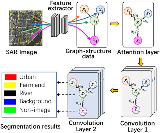
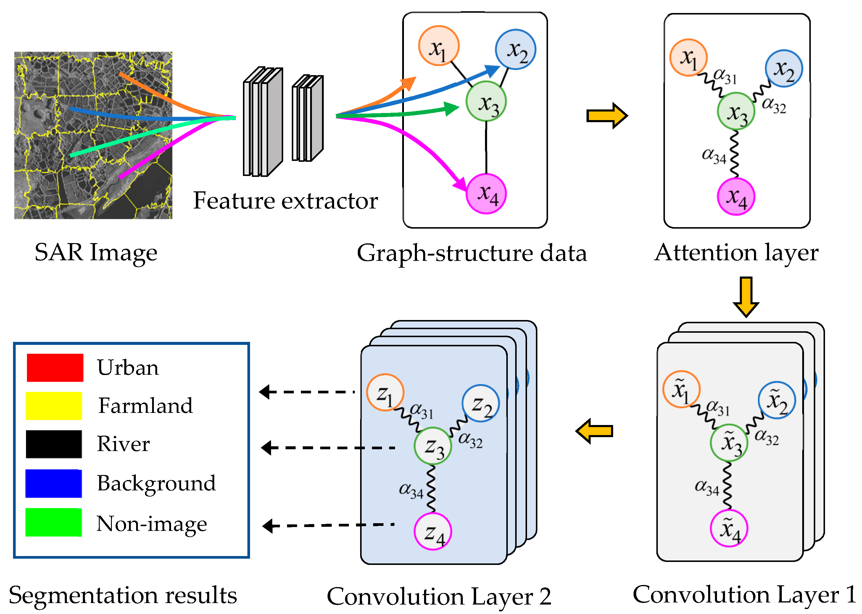
This paper presents a new Attention GCN model (AGCN) that resolves this problem. The structure of the AGCN for SAR image segmentation is shown in Figure 1. The method firstly uses an over-segmentation algorithm SLIC to segment the input image into a set of superpixels. It models the input SAR image into a graph, where a node represents a superpixel and adjacent superpixels are connected with the edges. Then, a supervised CNN is employed to extract the feature vectors of superpixels. The AGCN shown in Figure 1 contains an attention layer and two graph convolution layers, where ${\tilde{x}}_i$ in Convolution Layer 1 represents the feature of node $i$ after the first convolution and $z_i$ indicates the predicted class of node $i$ by the second convolutional layer. The attention layer aims to calculate the attention coefficients between adjacent nodes, i.e., ${\alpha }_{ij}$, and revise the graph Laplacian. The subsequent graph convolutional layers explore the hidden feature of nodes and segment the nodes based on the updated graph Laplacian.

3.1. Graph Construction

In order to meet the real-time requirements in processing big SAR imagery data, we first need to over-segment the large-scale airborne SAR images into superpixels using the SLIC proposed in [10]. Compared with the rectangular patches frequently used in deep learning, superpixels can preserve the edge information of the scene, while effectively speeding up the segmentation algorithm. We represent the superpixels obtained from a SAR image as $r_j,j=1,\cdots ,N$, where $N$ is the number of superpixels.

An input SAR image is modelled as an undirected graph model $G\left(V,E\right)$, where each superpixel corresponds to a vertex. Each node is only connected to its neighbouring nodes. In other words, those nodes sharing common boundaries will be connected by edges. $V$ and $E$ respectively represent the set of all the vertices and edges.

In order to extract the feature of irregular superpixels using CNN, we place each superpixel into a rectangular patch. The centroid of the superpixel is located at the central of the patch. The pixels in the patch not belonging to the superpixel regions are set as zero. The CNN network consists of several convolutional layers, fully connected layers, and a SoftMax layer, which are updated with a random gradient descent method. After training, the convolutional layers and fully connected layers form the feature extraction network, and the feature vector of superpixel $r_i$ is expressed as $x_i\in {ℝ}^C$.

3.2. Superpixel-Based Voting

The ground truth in the training set only provides the pixel-wise labels. Although SLIC considers the various text features and boundary information in the process of over-segmentation, it is still possible to include different kinds of pixels in one superpixel. Hence, we utilize a majority voting strategy to obtain the labels of superpixels. Let $G$ denote the ground truth of a training image. ${\left\{{\widehat{r}}_j\right\}}_{j=1}^N$ represents the corresponding area of ${\left\{r_j\right\}}_{j=1}^N$ in the ground truth $G$. There are $M$ pixels in the superpixel, i.e., $M=\left|{\widehat{r}}_j\right|$, and the category of the m^th pixel is represented as $l_m,m=1,\dots ,M$. Then, the number of pixels in ${\widehat{r}}_j$ belonging to each category is counted, and the most frequent class will be selected as the category of $r_j$, represented as:

$$y_j=\underset{r=\left\{1,\dots ,K\right\}}{\mathrm{argmax}}{\displaystyle \sum _{m=1}^{M}sign\left(l_m=r\right)},$$

(10)

where $sign(·)$ denotes an indicator function, $sign\left(turn\right)=1$, $sign\left(false\right)=0$. $r$ is the possible class in the training dataset. The same voting scheme is applied in all the superpixels in both the training and testing dataset to acquire their labels.

3.3. Attention Mechanism Layer

The first layer of the network is the attention layer. Similar to the GAT model, we inject the graph structure into the mechanism by performing masked attention; we only compute the attention coefficients between adjacent nodes. In all the follow-up experiments, these will be exactly the first-order neighbours of node $i$. In our framework, the attention coefficients $e_{ij}$ is defined as:

$$e_{ij}={\overrightarrow{a}}^T\left({\overrightarrow{x}}_i\Vert {\overrightarrow{x}}_j\right),$$

(11)

where $\overrightarrow{a}\in {ℝ}^{2C}$ is a $1\times 2C$ parameter vector, representing the weights of diverse elements of the feature vectors. $\overrightarrow{a}$ is essentially a linear combination of the combined features. $e_{ij}$ indicates the importance of node j to node $i$ in the task of segmentation. The more important node $j$ is to node $i$, the greater the attention coefficient e_ij. Note that the GAT model requires a learnable parameter matrix $W$ to transform linearly the features of nodes into higher-level features before we calculate attention coefficients in Equation (8). The linear transformation matrix $W$ is also the convolution kernel in Equation (9). The input features extracted by CNN already obtain sufficient expressive power, and there is no need to transform the feature again. Furthermore, the subsequent convolution operations are also linear transformations for node features, so the transformation here is repetitive and redundant. It is also difficult to ensure the simultaneously accuracy of the convolution operation and the linear transformation during the training process.

Then, we employ the SoftMax function to normalize the attention coefficients of each node:

$${\alpha }_{ij}={\mathrm{softmax}}_j\left(e_{ij}\right)=\frac{\exp \left(\mathrm{LeakyReLU}\left({\overrightarrow{a}}^T\left({\overrightarrow{x}}_i\Vert {\overrightarrow{x}}_j\right)\right)\right)}{{\displaystyle {\sum }_{j\in N_i}\exp \left(\mathrm{LeakyReLU}\left({\overrightarrow{a}}^T\left({\overrightarrow{x}}_i\Vert {\overrightarrow{x}}_j\right)\right)\right)}},$$

(12)

where $N_i$ are all the neighbourhoods of node i in the graph. ${\alpha }_{ij}$ represents the normalized attention coefficient. $\mathrm{LeakyReLU}(·)$ indicates the activation function LeakyReLU. Normalization realizes ${\displaystyle {\sum }_{j\in N_i}{\alpha }_{ij}}=1$ and makes coefficients easily comparable across different nodes. Let ${\overrightarrow{\alpha }}_i=\left\{{\alpha }_{i1},{\alpha }_{i2},,\dots ,{\alpha }_{iN}\right\}$ represent the attention coefficient vector of node $i$. If node $j\notin N_i$, the corresponding attention coefficient ${\alpha }_{ij}=0$, and we define ${\alpha }_{ii}=1$. The coefficient vectors of all the nodes form the matrix of attention coefficients $\alpha =\left\{{\overrightarrow{\alpha }}_1,{\overrightarrow{\alpha }}_2,,\dots ,{\overrightarrow{\alpha }}_N\right\}$. It can be seen that $\alpha$ is a symmetric matrix, i.e., ${\alpha }_{ij}={\alpha }_{ji}$.

In the following spectral convolution layers, we adopt the definition used in Equation (7), where the convolution of a signal $X\in {ℝ}^{N\times C}$ (a C-dimensional feature vector for each node) and $F$ filters is defined as $Z=({\tilde{D}}^{-1/2}\tilde{A}{\tilde{D}}^{-1/2})X\mathsf{\Theta }$. ${\tilde{D}}^{-1/2}\tilde{A}{\tilde{D}}^{-1/2}$ is named as the generalized graph Laplacian, and it contains the structure information of the graph. In order to make the learned attention coefficients guide the following convolution operation, we utilize the attention coefficient matrix to update ${\tilde{D}}^{-1/2}\tilde{A}{\tilde{D}}^{-1/2}$:

$$\widehat{A}={\tilde{D}}^{-1/2}\tilde{A}{\tilde{D}}^{-1/2}\ast {\mathsf{\alpha }}^T,$$

(13)

where $\ast$ is the Hadamard product, representing the product of the corresponding elements of two matrices. The above process is the attention layer of the AGCN network. The elements of the updated generalized graph Laplacian $\widehat{A}$ not only represent the structural information of the graph model (which nodes are connected), but also denotes the relationship between the two adjacent nodes in the feature space. Subsequent convolution layers can pay more attention to important nodes with the following expression:

$$Z=\left({\tilde{D}}^{-1/2}\tilde{A}{\tilde{D}}^{-1/2}\ast {\mathsf{\alpha }}^T\right)X\mathsf{\Theta }=\widehat{A}X\mathsf{\Theta },$$

(14)

3.4. Attention Graph Convolutional Network

In this section, we will provide a multi-layer attention GCN for node segmentation on graphs. In the GAT model, each layer needs to calculate the attention coefficients before convolution. However, we find that this improvement leads to the decline in performance of GAT when segmenting many SAR images. It is because much context information from adjacent superpixels has flown into the central superpixels after the first convolution operation. In the second convolution layer, these features are then utilized to calculate the attention coefficients. The existence of background information makes it impossible for coefficients to represent accurately the relationship between two nodes in feature space. The inaccurate coefficients further cause more noise in the following convolution operation. These errors are propagated to the next convolution layer. With the layers being deeper, the errors in the coefficients and nodes’ features will expand exponentially, leading to a sharper decline in the final segmentation. Moreover, there are more speckle noise and clusters in SAR images, making the situation even worse.

Unlike GAT, AGCN shown in Figure 1 is composed of an attention layer and two convolution layers. The attention layer aims at calculating attention coefficients. These coefficients are used to guide the subsequent convolution layers by revising the graph Laplacian. As no background information is contained in nodes’ features, the coefficients can accurately indicate the relationship between two adjacent superpixels in the feature space.

Specifically, an input SAR image is over-segmented into $N$ superpixels, and the feature vector set is represented as $X=\left\{{\overrightarrow{x}}_1,{\overrightarrow{x}}_2,\dots ,{\overrightarrow{x}}_N\right\}$. As depicted in Figure 1, this AGCN model contains an attention layer and two graph convolutional layers. The attention layer aims at optimizing the generalized graph Laplacian $\widehat{A}$. Then, the input graph-structure signal propagates layer by layer with the following rule:

$$Z^{l+1}=\sigma \left(\widehat{A}{Z}^l{\mathsf{\Theta }}^l\right),$$

(15)

where ${\mathsf{\Theta }}^l$ is the trainable weight matrix of the $l^{th}$ graph convolution layer; $\sigma (·)$ represents an activation function. $Z^l\in {ℝ}^{N\times C}$ denotes the input signal of the $l^{th}$ layer. In the first convolutional layer, $Z^{\left(0\right)}=X$, and the learnable parameter matrix is ${\mathsf{\Theta }}^{\left(0\right)}\in {ℝ}^{C\times C\prime }$. $C\prime$ indicates the number of the convolution kernels and is equal to the dimension of the output features of nodes.

Similarly, ${\mathsf{\Theta }}^{\left(1\right)}\in {ℝ}^{C\prime \times F}$ represents the parameter matrix of the second convolutional layer, and $F$ is the dimension of each node’s feature in the output. The second convolutional layer outputs $Z^1\in {ℝ}^{N\times F}$, where $Z^1={\left\{{\overrightarrow{z}}_1,{\overrightarrow{z}}_2,\dots ,{\overrightarrow{z}}_N\right\}}^T$. Finally, we utilize the SoftMax function to normalize ${\overrightarrow{z}}_i$. The $f_{\mathrm{th}}$ element of ${\overrightarrow{z}}_i$ is expressed as ${\overrightarrow{z}}_i\left(f\right)$, meaning the probability that node i belongs to the class $f$. The AGCN model is trained to minimize cross-entropy on the training nodes. The loss function $L$ is defined as:

$$L=-{\displaystyle \sum _{l\in y}{\displaystyle \sum _{f=1}^F{y}_{\left(l,f\right)}\ln {\overrightarrow{z}}_i\left(f\right)}},$$

(16)

where $y=\left\{y_1,y_2,\dots ,y_N\right\}$ indicates the one-hot encoding labels of N superpixels and $y_{\left(l,f\right)}\in \left\{0,1\right\}$ is the $f_{\mathrm{th}}$ element of $y_i$. Parameters $\overrightarrow{a}$, ${\mathsf{\Theta }}^{\left(0\right)}$ and ${\mathsf{\Theta }}^{\left(1\right)}$ are then updated using the Adam Stochastic Gradient Descent (SGD) optimizer.

The pseudocode of the proposed method is presented in Algorithm 1, which explains the training of AGCN in detail.

Algorithm 1: Training AGCN for Image Segmentation.

4. Results

In this section, we will first describe the datasets and evaluation measures used in the experiments. The empirical evaluation and analysis of the proposed model against the state-of-the-art methods on high-resolution SAR images are then discussed.

4.1. Data Description

Two airborne SAR databases were used to evaluate the segmentation performance of the proposed method, which were the Fangchenggang and Pucheng datasets. The Fangchenggang dataset was acquired from Fangchenggang (N21°41′22.66″, E108°21′2.64″), Guangxi Province, China, in March 2016. The imaging range of this database was about 30 × 30 km with a resolution of 2 m, and the image size was 561 × 709 in pixels. There were in total 144 images in the dataset, and 28 of them were selected as the training images. These images contained five classes: farmland, river, urban, background, and non-image. Non-image refers to those unscanned areas during the imaging, whose pixel values were zero. Three exemplar images and the corresponding ground truth maps are illustrated in Figure 2. In the ground truth, different land-use categories were marked with various colours: red, yellow, black. blue and green, respectively.

Table 1. The numbers of superpixels of five classes in the training and testing set.

	Farmland	River	Urban	Background	Non-Image
Train Test	1835 2624	3573 18,042	1654 3278	6899 33,994	1825 10,906

gives the numbers of the superpixels of five categories in the training and testing sets. As can be seen, the superpixels belonging to urban, farmland, and river basically had similar numbers in both the training and testing sets. The quantity of background superpixels was much larger than that of the other four categories, which conforms to the practical condition. In most of the practical application, we were only interested in a small part of land species in the large scene.

The Pucheng dataset was collected from Pucheng (N34°50′9″, E109°32′37″) in Shanxi Province, China, using the airborne SAR sensor operating in the Ka band, spotlight mode and VV single polarization. It contained 85 high quality SAR images, where 24 images were selected as the training data and the others formed the testing data. Each image was 588 × 892 pixels, and the resolution was 1 m. As shown in Figure 3, the Pucheng dataset included mainly two representative land-use categories: farmland and urban.

4.2. Evaluation Metrics

We introduced pixel-wise Overall Accuracy (OA) [32], Overall Precision (OP) [33], F1-score [34] and Cohen’s kappa coefficient (κ) [35] to evaluate the segmentation results quantitatively. Among them, recall refers to the ratio of the pixels predicted correctly in all the pixels in the ground truth, and precision corresponds to the proportion of the pixels correctly assigned in all the segmentation results. OA and OP are defined as the weighted average recall and precision, respectively. The F1-score is the weighted harmonic of precision and recall as:

$$F_1=\frac{2\times precision\times recall}{precision+recall},$$

(17)

A larger F1-score indicates the better performance of the segmentation algorithm. The kappa coefficient is defined as:

$$\mathrm{Kappa}=\frac{p_o-p_e}{1-p_e},$$

(18)

where $p_o$ is the relative agreement between the segmentation results and the real labels; $p_e$ is the hypothetical probability of a chance agreement. A kappa coefficient closer to one denotes better agreement between the results and ground truth.

4.3. Implementation Details

Whether in the training or testing stage, all the SAR images and the corresponding ground truths were first over-segmented to the superpixels using SLIC [36]. According to our experiments, the superpixels approximately containing 800 pixels could better retain the shape of rivers and urban areas. Hence, we set each superpixel to contain an average of 800 pixels, and the compactness of the SLIC was 0.5. In other words, each SAR image from the Fangchenggang and Pucheng datasets was approximately segmented into 500 and 800 superpixels, respectively.

The shape of superpixels was irregular, and CNN could not directly extract their features. We placed each superpixel into a patch before feature extraction. In order to guarantee that the patch could accommodate a superpixel, its size had to be larger than the superpixels, which was set as 32 × 32 in this paper.

Table 2. The parameters of the CNN-based feature extraction network.

Input 32 × 32 Superpixel

3 × 3 Conv. 20, stride 1, LeakyReLU

3 × 3 Conv. 40, stride 2, LeakyReLU

3 × 3 Conv. 80, stride 2, LeakyReLU

2 × 2 Max-pool, stride none

100 fc LeakyReLU

Output 1 × 100 feature vector

shows the architecture and hyperparameters of the CNN based feature extractor. The feature extraction network consisted of three convolution layers, one pooling layer and one fully connected layer. Each convolution layer contained a Batch Normalization (BN) operation. The BN operation normalizes the data in each mini batch, changing its mean to zero and its variance to one. It can prevent gradient explosion or vanishing during training and accelerate the speed of training. Leaky Rectified Linear Unit (ReLU) (leak rate = 0.2) was adopted as the activation function. The last layer of CNN was a fully connected layer. In the process of training, a SoftMax classifier was added to the last layer. Adam was used as the optimizer, and the learning rate was set to 0.003. This CNN based feature extractor can convert each superpixel into a 1 × 100 feature vector.

The AGCN network used in the experiment consisted of one attention layer and two graph convolution layers. The first spectral convolution layer had eight convolution filters, denoted as $W^{\left(0\right)}\in R^{100\times 8}$, so that this layer output eight channel features. The second spectral convolution layer output the classification probability vector, so the number of filters remained consistent with that of the land-cover types. For example, in the experiments on Fangchenggang, the second layer had five filters, described by $W^{\left(1\right)}\in R^{8\times 5}$. For the Pucheng dataset, this layer had two learnable filters. ReLU was used as the activation function in all the layers. AGCN was trained with the learning rate = 0.001 and the Adam optimizer.

4.4. Experiments on the Fangchenggang Dataset

This section validates the performance of the proposed AGCN and compares it with several other methods. The experiment consisted of two parts. The first part used all 28 images in the training set to train the feature extraction network and the AGCN. In the second part, seven images in the training set were selected to train the networks, and the remaining images were put into the test set. In this way, we could verify the performance of our method when the number of training samples was small.

4.4.1. Experiments Using the Complete Training Set

We test our AGCN algorithm and compare the experimental results with several methods in this section, such as GAT, GCN, CNN, AlexNet [37], Deep Convolutional Autoencoder (DCAE) [38] and SegNet [39]. Among them, CNN was composed of the feature extractor shown in Table 2 and a multi-classifier. The only difference between AGCN and GCN was that the former introduced an attention layer before two spectral convolution layers. The comparison between two networks allowed us to explore whether or not introducing attention coefficients could improve the segmentation results. GAT also contained two convolution layers. The attention coefficients were calculated in each layer based on the linearly transformed input features. Beyond that, the other hyperparameters of GAT were the same as for AGCN.

AlexNet refers to the classification method composed of AlexNet [37] and a fully connected network [40]. During the training of the network, the parameters of convolution and pooling layers in AlexNet were fixed, and the patches from the training set were used to train the fully connected layers. According to the suggestion of [37], the input patches with a size of 21 × 21 were cropped from the training images with a step size of one. AlexNet was trained with the mean squared error function, learning rate = 0.0001, batch size = 330 and training epoch = 40.

DCAE is a classification network based on the auto-encoder proposed in [38]. DCAE employs a dual-layer sparse autoencoder to optimize the Grey-Level Co-occurrence Matrix (GLCM) and Gabor features, and then, a fully connected layer with SoftMax activation functions is used to classify the features. DCAE in this section adopted the same architecture and hyperparameters as [12].

SegNet is a pixel-wise deep neural network for semantic segmentation proposed in [39], which adopts the “encoder + decoder” structure. The encoder uses 13 convolution layers of VGG16 pre-trained on ImageNet to extract features. The decoder maps feature vectors to segmentation results through deconvolution and a SoftMax classifier. Experimental results showed that a larger patch size more easily caused unstable convergence of the training. Hence, we finally set the patch size to 16 × 16. The learning rate was 0.01, the regular regularization parameter = 0.0005, batch size = 300, and training epoch = 5.

Table 3. Comparison of the overall segmentation performance with six state-of-the-art methods. GAT, Graph Attention Network.

	AGCN	GAT	GCN	CNN	AlexNet	DCAE	SegNet
OP (%)	90.55	89.47	89.53	81.62	77.29	78.78	85.85
OA (%)	90.74	89.79	89.43	81.10	76.15	79.75	84.90
F1-score (%)	90.44	89.43	89.37	81.03	76.51	79.08	85.16
κ	0.8444	0.8284	0.8266	0.6974	0.6303	0.6725	0.7579

shows the performance comparison of the above seven methods on the test set when all the training data were used to train the algorithms. AGCN achieved the highest OA, OP, F1-score and kappa coefficients. As classification methods, CNN, AlexNet and DCAE did not take the spatial relationship between neighbour units into consideration during segmentation. Hence, there existed a big gap between their segmentation performance and that of the other three spectral convolution based methods. Moreover, the results of AGCN, GAT and GCN were much better than the methods based on the conventional convolution methods, indicating that spectral convolution was more suitable for processing graph-structure data.

The introduction of the attention mechanism made GAT’s OA, F1-score and kappa coefficients better than those of GCN, but still lower than those of AGCN. That was because there was much background information from the neighbouring superpixels in the central superpixel during the first convolution operations, and these inaccurate representations were then utilized to calculate the attention coefficients in the second convolution layers, resulting in more noise in the final segmentation results. Compared with GCN and GAT, AGCN added a separate attention layer to calculate the attention coefficients before convolution operations, ensuring that the coefficients accurately indicated the relationship between two superpixels in the feature space. The experiment results also proved the effectiveness of this improvement.

Table 4. Comparison of the pixel-wise F1-scores for individual classes with six state-of-the-art methods.

Class	AGCN	GAT	GCN	CNN	AlexNet	DCAE	SegNet
Urban Farmland River Background Non-image	68.13 70.96 85.68 92.59 99.11	69.13 68.18 82.12 92.22 97.59	70.08 71.80 81.94 91.24 99.27	58.46 56.64 58.65 87.40 89.76	45.79 25.12 70.15 80.69 98.92	54.86 27.89 71.01 83.79 98.33	61.46 52.56 75.00 90.43 99.04

shows the results of the seven methods on different land-cover classes. For urban, farmland and non-image areas, GCN’s F1-scores were slightly higher than AGCN’s. AGCN achieved the best segmentation performance for river and background areas. There existed many irregular rivers areas in the Fangchenggang dataset. The F1-scores of CNN, AlexNet, DCAE and SegNet for the river area were all below 80%. In comparison, AGCN’s F1-score for river regions reached 85.68, much larger than those of the other six methods. This experimental outcome demonstrated that our algorithm can better consider the context of superpixels during the segmentation.

In order to compare the segmentation results intuitively, we display the maps of various methods in Figure 4. Figure 4a,b shows the SAR image and the ground truth, where the river areas and some shadows in background areas are almost indistinguishable without considering the context information. GAT and GCN confused large mountain shadow areas with river areas, while AGCN had fewer areas of confusion. This demonstrated that the proposed AGCN could effectively make use of adjacent superpixels’ features to improve the segmentation accuracy. As AlexNet, DCAE and SegNet predicted each pixel separately, their results had more noise and neglected spatial consistency.

4.4.2. Experiments on Part of Training Set

In this section, the training images are reduced to seven, and the remaining training images are used as the testing images to verify the segmentation performance of AGCN with less training samples.

Table 5. Comparison of the overall segmentation performance with four state-of-the-art methods.

	A-GCN	GAT	GCN	CNN	SegNet
OP (%)	86.60	59.87	85.91	81.64	84.59
OA (%)	87.07	63.90	85.97	80.32	84.35
F1-score (%)	86.55	57.99	85.97	80.59	84.31
κ	0.7862	0.3756	0.7759	0.6940	0.7508

shows the segmentation results of AGCN, GAT, GCN, CNN and SegNet. It can be seen that the accuracy of all the methods decreased due to the reduced number of training images. However, AGCN still achieved the best performance in this condition. Taking F1-scores as an example, AGCN was 86.55, higher than GCN (85.97), GAT (57.99), CNN (80.59) and SegNet (84.31). Compared with the F1-scores shown in Table 3, GAT suffered the biggest drops, declining from 89.43 to 57.99. The reduction of the training samples resulted in the deterioration of CNN in the feature extraction, and more noise exited in the superpixels’ features. As GAT calculated the attention coefficients in each layer, the inaccurate representations of nodes from the current layer would be propagated to the next convolution layer. With the layers being deeper, the errors in the coefficients would expand exponentially, leading to a sharper decline in the segmentation results.

Table 6. Comparison of pixelwise F1-scores for individual classes with four state-of-the-art methods.

Class	A-GCN	GAT	GCN	CNN	SegNet
Urban Farmland River Background Non-image	67.74 56.96 78.54 90.57 96.99	03.85 00.01 74.50 85.50 00.00	68.70 62.67 75.67 89.17 97.22	55.40 50.13 69.05 83.97 98.42	59.91 67.05 73.37 87.14 98.58

compares the F1-scores of AGCN, GAT, GCN, CNN and SegNet for five categories. Farmland was the most difficult class to segment in this dataset. AGCN generated the best performance for rivers and background areas. GCN gave the optimal results for urban, and SegNet had advantages in segmenting the farmland and non-image regions. Urban and farmland categories were seriously confused by GAT. The above comparison proved that our attention layer could effectively strengthen the segmentation performance of AGCN under less training samples.

Figure 5a,b displays a SAR image in the Fangchenggang dataset and its corresponding ground truth map. This image mainly includes a large river area with complicated shapes. In addition, the roads are annotated as urban areas in the ground truth map. Figure 5c–f shows the results of AGCN, GAT, GCN and SegNet. In the results of GAT, a large part of the river areas located at the bottom of the image was misclassified as non-image areas. Note that some shadows of mountains in the lower right corner of the image were misclassified as rivers in both GAT and GCN’s results. SegNet’s results had much noise in the river regions, whereas our segmentation maps were closer to the ground truth, indicating that our method could yield satisfactory results in the absence of labelling information.

4.5. Experiments on the Pucheng Dataset

This section focuses on validating the effectiveness of the proposed algorithm on images captured by different SAR sensors. As shown in

Table 7. Comparison of different segmentation methods on the Pucheng dataset.

Methods	OP (%)	OA (%)	F1-score (%)	κ	F1-Score (%)
					Urban	Farmland
AGCN	95.57	94.61	94.90	0.7604	79.08	96.90
GAT	95.16	93.43	93.93	0.7238	76.04	96.19
GCN	95.40	94.38	94.70	0.7512	78.28	96.77
CNN	92.86	91.60	92.07	0.6272	67.44	95.18
SegNet	94.39	94.07	94.20	0.7162	74.97	96.63

, we compared our algorithm with four state-of-the-art methods on the Pucheng dataset, i.e., GAT, GCN, CNN and SegNet. The AGCN algorithm obviously achieved the highest OA and kappa of 94.61% and 0.7604. The kappa coefficient of GAT (0.7238) was lower than that of GCN (0.7512), indicating that the attention coefficients in GAT were susceptible to speckle noise in the SAR images. The traditional CNN failed to consider the effect of the neighbouring nodes, hence having the minimum F1-score and kappa. These results demonstrated that the proposed AGCN had good practicability and could be used to segment the images captured by different SAR sensors.

To demonstrate the segmentation results, we also display the land-use segmentation maps of multiple methods in Figure 6. Figure 6a,b shows a SAR image from the Pucheng dataset and its corresponding ground truth map. Figure 6c–f shows the results of AGCN, GAT, GCN and SegNet, respectively. More farmland areas can be seen in Figure 6d–f to be misclassed as urban. Our AGCN algorithm yielded the best segmentation performance, which was close to the ground truth. As SegNet segmenting of the image took the 16 × 16 patch as the unit, it could only consider the context information inside a patch, with noise in the segmentation results. These results proved that our AGCN model could provide reliable segmentation results for various SAR images.

5. Discussion

5.1. Selection of Superpixel’s Size

The size of the superpixel determines the resolution of the segmentation results. If the superpixels are too large, the segmentation results will lose much edge information. Instead, too small superpixels will introduce more noise into the results and increase the computational burden of the segmentation algorithms in big data. Figure 7 illustrates the F1-scores and kappa coefficients of AGCN on the Fangchenggang dataset using different sizes of superpixels. The abscissa of Figure 7 is the number of superpixels contained in one test image, ranging from 400 to 2000. The larger the number, the smaller the superpixel size. Since the image of Fangchenggang dataset was 561 × 709, it means that the number of pixels included in a superpixel approximately ranged from 200 to 1000.

When the number of superpixels was greater than 800, the accuracy of the AGCN was rapidly degraded. AGCN had two convolutional layers, which means that each superpixel could only obtain the background information from its second-order neighbourhood (including those nodes neighbouring it and the nodes sharing common boundaries with its neighbouring nodes). The small superpixel will curtail the scope of node connection, so that the superpixel can only get limited background information. The results will have more noise and neglect spatial consistency. When the number of superpixels was between 500 and 800, AGCN could achieve better segmentation results. Therefore, in our experiment section, each SAR image of the Fangchenggang dataset was over-segmented into about 500 superpixels.

5.2. Performance of AGCN for Different SNR Values

Speckle noise occurs in SAR images when the resolution cell dimensions are much larger than the wavelength of the incident electromagnetic field [41]. The existence of speckle will degrade the human interpretation and the computer-aided scene analysis in segmentation. Therefore, for a segmentation algorithm, it is of crucial importance to maintain good performance under different Signal-to-Noise Ratios (SNR). This section aims to quantify the performances of our method for different SNR values.

First, we added multiplicative noise to all SAR images from the Fangchenggang dataset using the equation $J=I+n*I$, where $n$ is uniformly distributed random noise with mean zero. $J$ and $I$ are the speckled images and the original SAR images, respectively. The SNR of the synthetic SAR image is defined as:

$$SNR={10}^{*}lo{g}_{10}\left[\frac{\mathrm{mean}{\left(I\right)}^2}{\mathrm{MSE}\left(I,J\right)}\right],$$

(19)

where $\mathrm{mean}(·)$ denotes the mean of image $I$ and $\mathrm{MSE}\left(I,J\right)$ represents the Mean Squared Error (MSE) between $I$ and $J$. The SNR of the speckled image was determined by the variance of the noise $n$. A higher value SNR indicates more speckle noise in the images. Parts of speckled images are given in Figure 8. Specifically, Figure 8a is the original SAR image, and Figure 8b,c shows two speckled images, whose SNR was five and three, respectively.

Then, AGCN, GAT, GCN and CNN were trained by the speckled training set and utilized to segment the speckled testing set, and the corresponding results are summarized in

Table 8. Comparison segmentation performance of four methods for different SNR values.

Method	SNR = 5		SNR = 3
	F1-Score (%)	κ	F1-Score (%)	κ
AGCN	87.46	0.8010	87.27	0.7984
GAT	87.23	0.7828	85.34	0.7670
GCN	86.34	0.7794	85.13	0.7601
CNN	58.50	0.4165	50.31	0.3522

. As can be seen from Table 8, the proposed AGCN method achieved the best F1-score and kappa coefficient gain over the other three methods. When the SNR value dropped from five to three, the increase in noise caused the performance of the four segmentation methods to decrease. AGCN’s F1-score decreased by 0.19 (from 87.46 to 87.27). The F1-scores of GAT, GCN and CNN decreased by 1.89, 1.21 and 8.19, respectively. This indicates that our algorithm exhibited stronger robustness to the noise thanks to the introduction of the separate attention layer.

Figure 9a shows a speckled image (SNR = 3), and its corresponding original SAR image is shown in Figure 4a. Figure 9b–d draws the segmentation results of the AGCN, GAT and GCN for the speckled image in Figure 9a. Referring to the ground truth in Figure 4b, GAT and GCN labelled many shadow regions of mountains as rivers. The results of AGCN contained fewer errors and were closer to the ground truth map. Furthermore, by comparing Figure 9b–d with Figure 4c–e, it can be seen that the results of AGCN were less affected by noise.

5.3. Computational Complexity

The computational complexity of each layer of GAT was $O(\left|V\right|CC\prime )+O(\left|\epsilon \right|C\prime )$, where C and $C\prime$ are the dimensions of the input feature and output feature, respectively. $\left|V\right|$ and $\left|\epsilon \right|$ denote the numbers of the nodes and edges in the graph. $O(\left|V\right|CC\prime )$ refers to computing attention coefficients, and $O(\left|\epsilon \right|C\prime )$ corresponds to the convolution operation. Since our attention layer omitted linear transformation before calculating attention coefficients, it had less computational complexity and could handle the big SAR data efficiently.

This section counts the running time required for different algorithms to segment all the test images of the Fangchenggang dataset.

Table 9. Comparison of the run time (seconds) with five state-of-the-art algorithms on the Fangchenggang dataset.

Class	AGCN	GAT	GCN	AlexNet	DCAE	SegNet
Time(s)	168.3 s	169.8 s	167.2 s	480.0	4219.0	3380.0

compares the time of the proposed method with that of the state-of-the-art methods. The experiment was implemented on the Ubuntu platform using Pytorch. The main configuration of the computer included 32 G memory, Intel (R) Xeon (R) CPU L5639 with 2.13GHz × 12 (Intel, Santa Clara, CA, USA) and Tesla K20c graphics (NVIDIA, Santa Clara, CA, USA).

As shown in Table 9, the running times of AGCN, GAT and GCN were far less than those of DCAE, AlexNet and SegNet. This demonstrated that taking superpixels as processing units could greatly reduce the computational complexity of the segmentation methods in big data. DCAE needs to extract Gabor and GLCM features, with costly computation. As a pixel-wise semantic segmentation network, SegNet employs deconvolution operations to encode the spatial context information of the pixels, which has a heavy computational burden. Moreover, as GAT needs to calculate the attention coefficients in each convolution layer, its computational time was slightly larger than that of AGCN and GCN, which was consistent with our theoretical analysis.

6. Conclusions

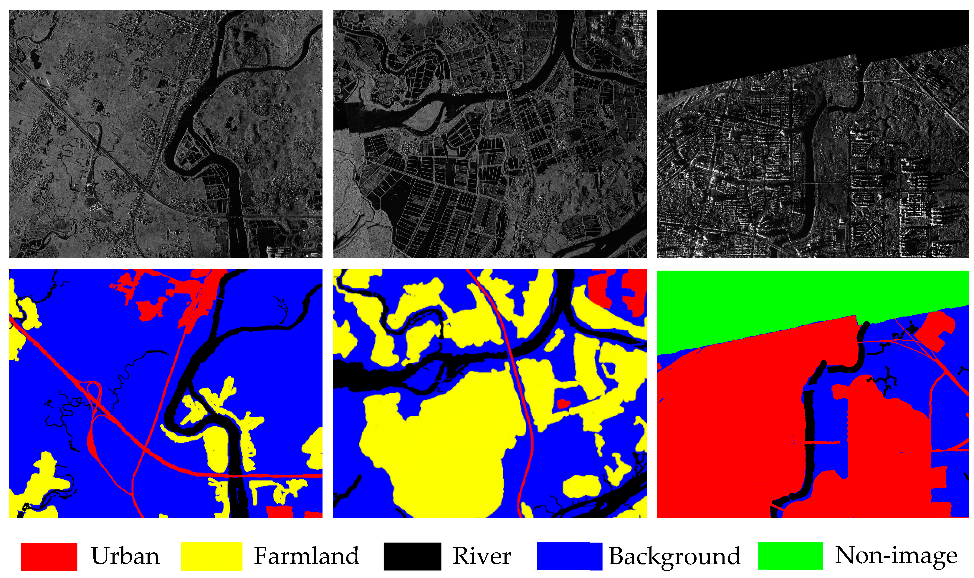
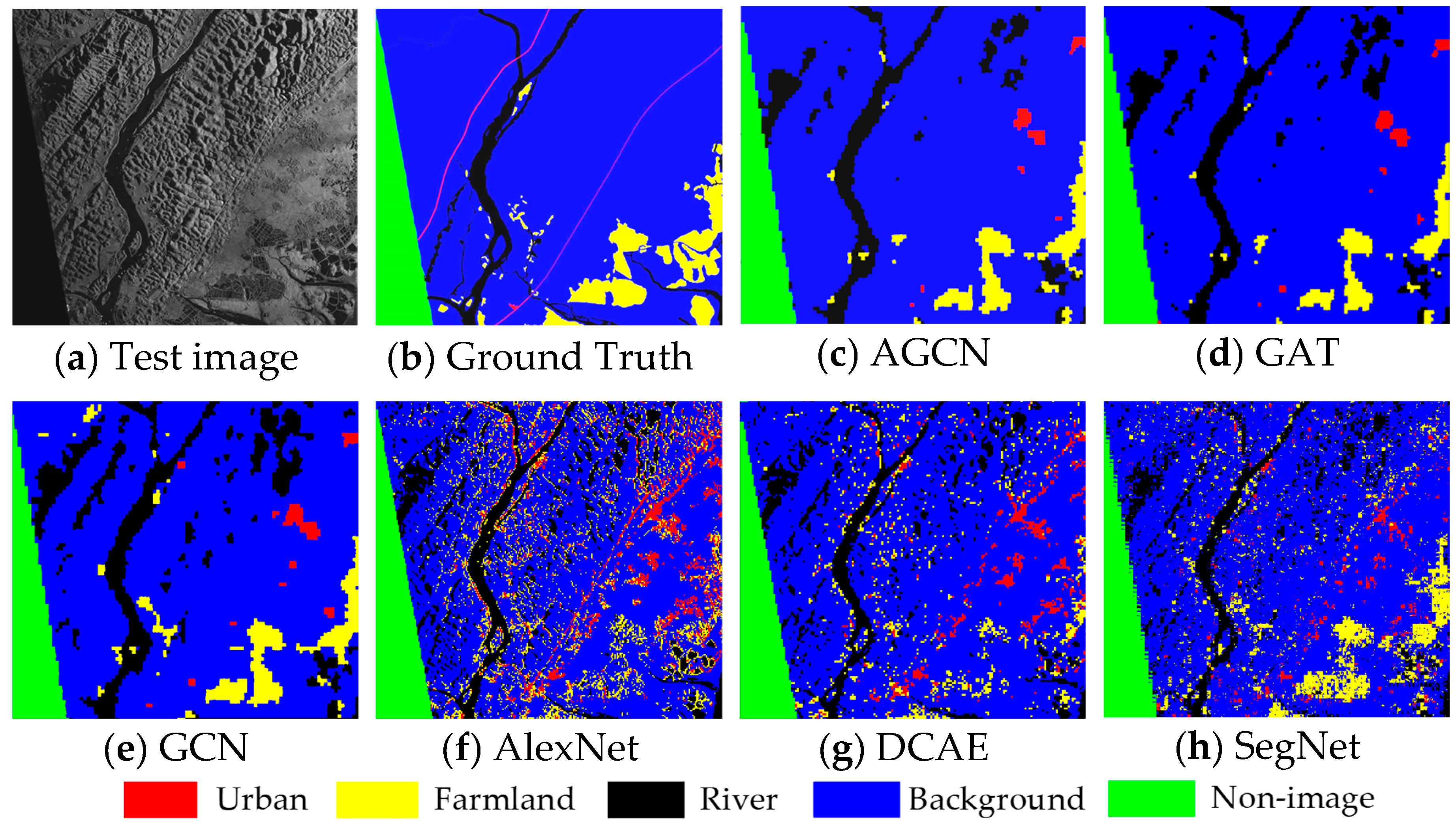
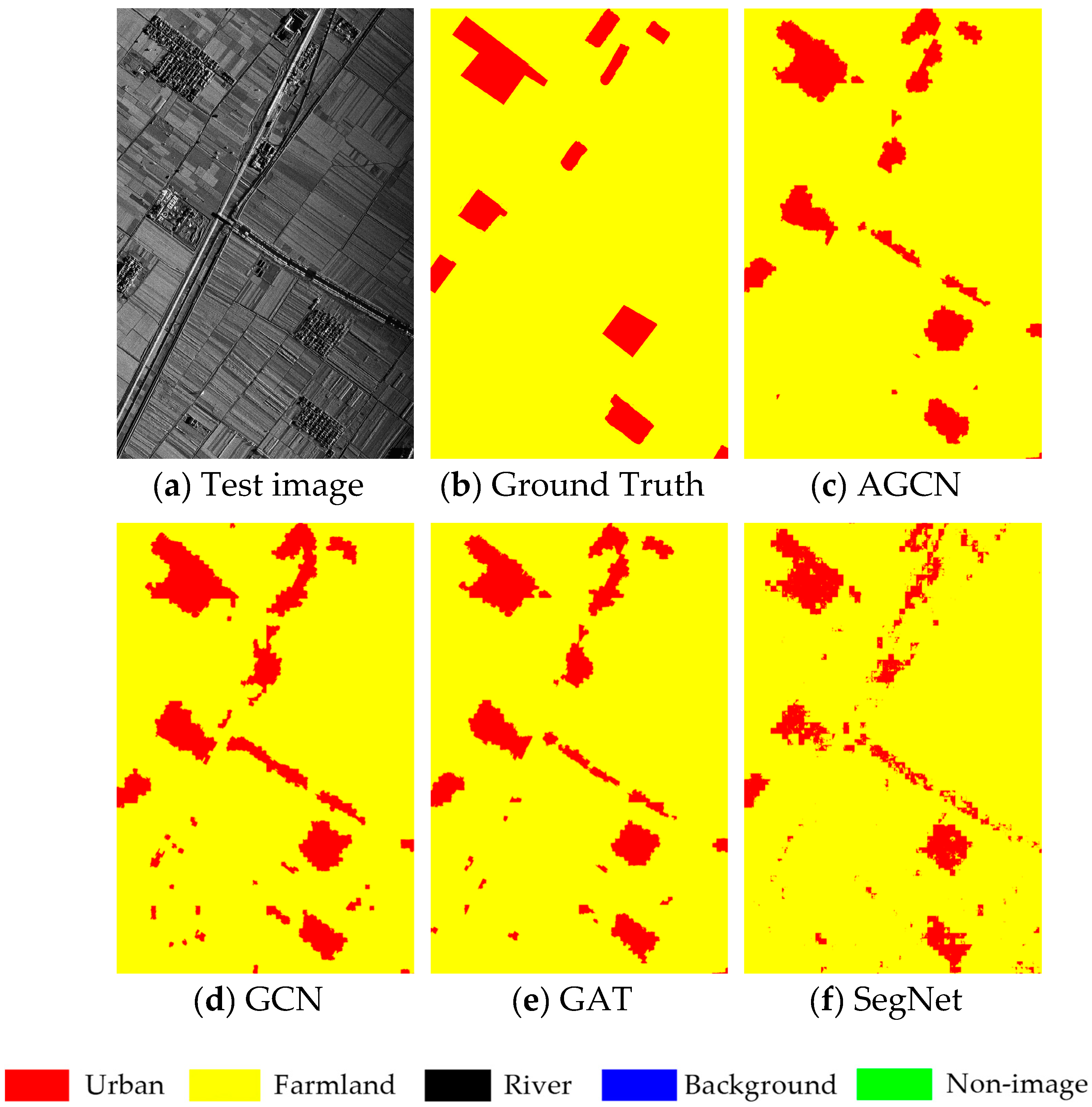
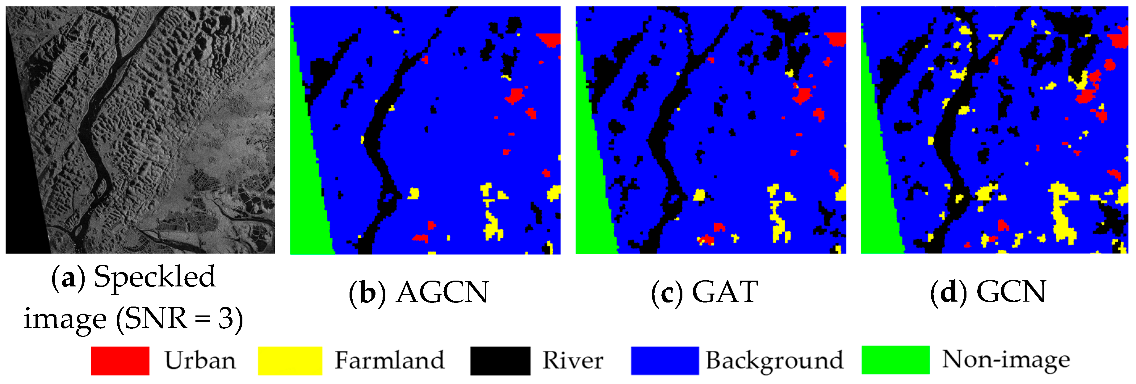
To address segmentation problems in big SAR data, we presented a novel Attention Graph Convolution Network (AGCN) in this study. In order to improve the efficiency of the segmentation algorithm, the input images were first over-segmented into superpixels, converted to graph-structured data. The previous spectral convolution methods generally ignored the various functions of the neighbouring nodes on the central nodes. In AGCN, an attention layer was introduced to calculate the attention coefficients of adjacent nodes before graph convolution operations. The greater the attention coefficients were, the greater the correlation there was between two nodes. The attention coefficients were utilized to update the generalized graph Laplacian, guiding the subsequent convolution operations to focus on the most relevant nodes to make decisions. AGCN can address the shortcomings of previous methods based on attention and spectral convolution. A number of experiments on two airborne SAR image datasets showed that: (1) The introduction of the attention layer improved the performance of the graph convolution networks. For SAR images with different scenes, AGCN could obtain higher segmentation accuracy and better preserve the neighbour consistency in the results. (2) The added attention layer did not introduce costly matrix operation. In the condition of using the same data and hardware configuration, our method required less computational time during the test stage than GAT and some common pixel-wise segmentation algorithms, e.g., SegNet.

In terms of limitations, it should be noted that different land-use categories in SAR images are in different scale spaces, while the superpixels used in AGCN only have one scale. Hence, AGCN is prone to errors when segmenting some thin areas, such as rivers and roads. In future research, we will attempt to improve the accuracy of the over-segmentation method and implement segmentation in multiple scale spaces in order to maintain high segmentation performance for all kinds of regions. Furthermore, the number of spaceborne SAR images is much larger than that of airborne images. We also plan to further reduce the computational complexity of the algorithm, so that it can better segment the large quantity of satellite images.

References

1. Chen, H.; Zhang, F.; Tang, B.; Yin, Q.; Sun, X. Slim and Efficient Neural Network Design for Resource-Constrained SAR Target Recognition. Remote Sens. 2018, 10, 1618. [Google Scholar] [CrossRef]
2. Fei, G.; Fei, M.; Wang, J.; Sun, J.; Yang, E.; Zhou, H. Semi-Supervised Generative Adversarial Nets with Multiple Generators for SAR Image Recognition. Sensors 2018, 18, 2706. [Google Scholar] [Green Version]
3. Gao, F.; Ma, F.; Wang, J.; Sun, J.; Zhou, H. Visual Saliency Modeling for River Detection in High-resolution SAR Imagery. IEEE Access 2018, 6, 1000–1014. [Google Scholar] [CrossRef]
4. Zhou, L.; Guo, C.; Li, Y.; Shang, Y. Change Detection Based on Conditional Random Field with Region Connection Constraints in High-Resolution Remote Sensing Images. IEEE J. Sel. Top. Appl. Earth Observ. Remote Sens. 2017, 9, 3478–3488. [Google Scholar] [CrossRef]
5. Mason, D.; Davenport, I.; Neal, J.; Schumann, G.; Bates, P.D. Nearreal-time flood detection in urban and rural areas using high resolution synthetic aperture radar images. IEEE Trans. Geosci. Remote Sens. 2012, 50, 3041–3052. [Google Scholar] [CrossRef]
6. Covello, F.; Battazza, F.; Coletta, A.; Lopinto, E.; Fiorentino, C.; Pietranera, L.; Valentini, G.; Zoffoli, S. COSMO-SkyMed—An existing opportunity for observing the Earth. J. Geodyn. 2010, 49, 171. [Google Scholar] [CrossRef]
7. Suykens, J.A.K.; Vandewalle, J. Least squares support vector machine classifiers. Neural Process. Lett. 1999, 9, 293–300. [Google Scholar] [CrossRef]
8. González, A.; Pérez, R.; Romero-Zaliz, R. An Incremental Approach to Address Big Data Classification Problems Using Cognitive Models. Cogn. Comput. 2019, 11, 347–366. [Google Scholar] [CrossRef]
9. Padillo, F.; Luna, J.M.; Ventura, S.A. grammar-guided genetic programing algorithm for associative classification in Big Data. Cogn. Comput. 2019. [Google Scholar] [CrossRef]
10. Achanta, R.; Shaji, A.; Smith, K.; Lucchi, A.; Fua, P.; Susstrunk, S. SLIC Superpixels Compared to State-of-the-Art Superpixel Methods. IEEE Trans. Pattern Anal. Mach. Intell. 2012, 34, 2274–2282. [Google Scholar] [CrossRef]
11. Lafferty, J.D.; Mccallum, A.; Pereira, F.C.N. Conditional Random Fields: Probabilistic Models for Segmenting and Labeling Sequence Data. Proc. ICML 2001, 3, 282–289. [Google Scholar]
12. Ma, F.; Gao, F.; Sun, J. Weakly Supervised Segmentation of SAR Imagery Using Superpixel and Hierarchically Adversarial CRF. Remote Sens. 2019, 11, 512. [Google Scholar] [CrossRef]
13. Liu, F.; Lin, G.; Shen, C. CRF learning with CNN features for image segmentation. Pattern Recognit. 2015, 48, 2983–2992. [Google Scholar] [CrossRef] [Green Version]
14. Guo, E.; Bai, L.; Zhang, Y.; Han, J. Vehicle Detection Based on Superpixel and Improved HOG in Aerial Images. In International Conference on Image and Graphics; Springer: Cham, Switzerland, 2017. [Google Scholar]
15. Xiang, D.; Tang, T.; Zhao, L.; Su, Y. Superpixel Generating Algorithm Based on Pixel Intensity and Location Similarity for SAR Image Classification. IEEE Geosci. Remote Sens. Lett. 2013, 10, 1414–1418. [Google Scholar] [CrossRef]
16. Micusik, B.; Kosecka, J. Semantic segmentation of street scenes by superpixel co-occurrence and 3D geometry. In Proceedings of the IEEE International Conference on Computer Vision Workshops, Kyoto, Japan, 27 September–4 October 2009. [Google Scholar]
17. Szummer, M.; Kohli, P.; Hoiem, D. Learning CRFs Using Graph Cuts. In Proceedings of the European Conference on Computer Vision, Marseille, France, 12–18 October 2008. [Google Scholar]
18. Zhong, P.; Wang, R. Learning conditional random fields for classification of hyperspectral images. IEEE Trans. Image Process. 2010, 19, 1890–1907. [Google Scholar] [CrossRef]
19. Gao, F.; Huang, T.; Sun, J. A New Algorithm for SAR Image Target Recognition Based on an Improved Deep Convolutional Neural Network. Cogn. Comput. 2018. [Google Scholar] [CrossRef]
20. Xu, L.; Clausi, D.A.; Li, F.; Wong, A. Weakly Supervised Classification of Remotely Sensed Imagery Using Label Constraint and Edge Penalty. IEEE Trans. Geosci. Remote Sens. 2017, 55, 1424–1436. [Google Scholar] [CrossRef]
21. Bruna, J.; Zaremba, W.; Szlam, A. Spectral Networks and Locally Connected Networks on Graphs. arXiv 2013, arXiv:1312.6203. [Google Scholar]
22. Defferrard, M.; Bresson, X.; Vandergheynst, P. Convolutional Neural Networks on Graphs with Fast Localized Spectral Filtering. In Proceedings of the Advances in Neural Information Processing Systems (NIPS 2016), Barcelona, Spain, 5–10 December 2016; pp. 3844–3852. [Google Scholar]
23. Kipf, T.N.; Welling, M. Semi-Supervised Classification with Graph Convolutional Networks. arXiv 2016, arXiv:1609.02907. [Google Scholar]
24. Duvenaud, D.K.; Maclaurin, D.; Aguileraiparraguirre, J.; Gomezbombarelli, R.; Hirzel, T.D.; Aspuruguzik, A.; Adams, R.P. Convolutional networks on graphs for learning molecular fingerprints. In Proceedings of the Advances in Neural Information Processing Systems (NIPS 2015), Montreal, Canada, 7–12 December 2015; pp. 2224–2232. [Google Scholar]
25. Atwood, J.; Towsley, D. Diffusion-convolutional neural networks. In Proceedings of the Advances in Neural Information Processing Systems (NIPS 2016), Barcelona, Spain, 5–10 December 2016; pp. 1993–2001. [Google Scholar]
26. Niepert, M.; Ahmed, M.; Kutzkov, K. Learning convolutional neural networks for graphs. In Proceedings of the 33nd International Conference on Machine Learning (ICML 2016), New York City, NY, USA, 19–24 June 2016; pp. 2014–2023. [Google Scholar]
27. Hamilton, W.; Ying, Z.; Leskovec, J. Inductive representation learning on large graphs. In Proceedings of the Advances in Neural Information Processing Systems (NIPS 2017), Long Beach, CA, USA, 3–9 December 2017; pp. 1024–1034. [Google Scholar]
28. Zhang, F.; Yao, X.; Tang, H.; Yin, Q.; Hu, Y.; Lei, B. Multiple Mode SAR Raw Data Simulation and Parallel Acceleration for Gaofen-3 Mission. IEEE J. Sel. Top. Appl. Earth Observ. Remote Sens. 2018, 11, 2115–2126. [Google Scholar] [CrossRef]
29. Petar, V.; Guillem, C.; Arantxa, C.; Adriana, R.; Pietro, L.; Yoshua, B. Graph Attention Networks. arXiv 2017, arXiv:1710.10903. [Google Scholar]
30. Shuman, D.I.; Narang, S.K.; Frossard, P. The emerging field of signal processing on graphs: Extending high-dimensional data analysis to networks and other irregular domains. IEEE Signal Process. Mag. 2013, 30, 83–98. [Google Scholar] [CrossRef] [Green Version]
31. Henaff, M.; Bruna, J.; LeCun, Y. Deep convolutional networks on graph-structured data. arXiv 2015, arXiv:1506.05163. [Google Scholar]
32. Martha, T.R.; Kerle, N.; Westen, C.J.V.; Jetten, V.; Kumar, K.V. Segment Optimization and Data-Driven Thresholding for Knowledge-Based Landslide Detection by Object-Based Image Analysis. IEEE Trans. Geosci. Remote Sens. 2011, 49, 4928–4943. [Google Scholar] [CrossRef]
33. Jie, G.; Wang, H.; Fan, J.; Ma, X. SAR Image Classification via Deep Recurrent Encoding Neural Networks. IEEE Trans. Geosci. Remote Sens. 2018, 56, 2255–2269. [Google Scholar]
34. Sasaki, Y. The truth of the F-measure. Teach. Tutor Mater. 2007, 1, 1–5. [Google Scholar]
35. Cohen, J. A coefficient of agreement for nominal scales. Educ. Psychol. Meas. 1960, 20, 37–46. [Google Scholar] [CrossRef]
36. Huang, Y.L.; Xu, B.B.; Ren, S.Y. Analysis and pinning control for passivity of coupled reaction-diffusion neural networks with nonlinear coupling. Neurocomputing 2018, 272, 334–342. [Google Scholar] [CrossRef]
37. Tian, T.; Chang, L.; Jinkang, X.; Ma, J. Urban Area Detection in Very High Resolution Remote Sensing Images Using Deep Convolutional Neural Networks. Sensors 2018, 18, 904. [Google Scholar] [CrossRef]
38. Geng, J.; Fan, J.; Wang, H.; Ma, X.; Li, B.; Chen, F. High-Resolution SAR Image Classification via Deep Convolutional Autoencoders. IEEE Geosci. Remote Sens. Lett. 2015, 12, 1–5. [Google Scholar] [CrossRef]
39. Badrinarayanan, V.; Kendall, A.; Cipolla, R. SegNet: A Deep Convolutional Encoder-Decoder Architecture for Image Segmentation. arXiv 2015, arXiv:1505.07293. [Google Scholar] [CrossRef] [PubMed]
40. Yue, Z.; Gao, F.; Xiong, Q. A Novel Semi-Supervised Convolutional Neural Network Method for Synthetic Aperture Radar Image Recognition. Cogn. Comput. 2019. [Google Scholar] [CrossRef]
41. Martino, G.D.; Iodice, A.; Riccio, D. Equivalent Number of Scatterers for SAR Speckle Modeling. IEEE Trans. Geosci. Remote Sens. 2014, 52, 2555–2564. [Google Scholar] [CrossRef]
Figure 1. Architecture of our SAR image segmentation approach based on Attention Graph Convolution Network (AGCN).
Remotesensing 11 02586 g001
Figure 2. Part of images and the corresponding ground truth maps from the Fangchenggang dataset.
Remotesensing 11 02586 g002
Figure 3. Four SAR images from the Pucheng dataset.
Remotesensing 11 02586 g003
Figure 4. Segmentation results of six models on the Fangchenggang dataset. (a) Input image; (b) ground truth; (c) AGCN; (d) GAT; (e) GCN; (f) AlexNet; (g) DCAE; (h) SegNet.
Remotesensing 11 02586 g004
Figure 5. Segmentation results of four models on the Fangchenggang dataset. (a) Input image; (b) ground truth; (c) AGCN; (d) GAT; (e) GCN; (f) SegNet.
Remotesensing 11 02586 g005
Figure 6. Segmentation results of four models on the Pucheng dataset. (a) Input image; (b) ground truth; (c) AGCN; (d) GAT; (e) GCN; (f) SegNet.
Remotesensing 11 02586 g006
Figure 7. Effect of superpixels’ sizes for the segmentation results of AGCN on the Fangchenggang dataset.
Remotesensing 11 02586 g007
Figure 8. The speckled images with different SNR values.
Remotesensing 11 02586 g008
Figure 9. Segmentation results of three models for a speckled image. (a) Speckled image (SNR = 3); (b) AGCN (c) GAT; (d) GCN.
Remotesensing 11 02586 g009