Article

Pixel Tracking to Estimate Rivers Water Flow Elevation Using Cosmo-SkyMed Synthetic Aperture Radar Data

1
Electromagnetic Laboratory, Engineering Faculty, Università degli Studi dell’Aquila, Piazzale E. Pontieri, 67100 Monteluco di Roio, L’Aquila AQ, Italy
2
Consiglio Nazionale delle Ricerche (CNR), Istituto di ricerca per la Protezione Idrogeologica (IRPI), via Madonna Alta, 126, 06128 Perugia, Italy
3
Science and Technology for Transportations Faculty, Università degli Studi “Giustino Fortunato”, viale Raffale Delcogliano, 12, 82100 Benevento, Italy
4
Center for Signal and Image Processing, Department of Electronic and Electrical Engineering, University of Strathclyde, Glasgow G1 1XW, UK
5
Engineering Faculty, Università degli Studi “Niccolò Cusano”, Via Don Carlo Gnocchi, 3, 00166 Roma, Italy
*
Author to whom correspondence should be addressed.
Current address: Via Luca Benincasa 21/B 06073 Corciano Perugia, Italy.
Remote Sens. 2019, 11(21), 2574; https://doi.org/10.3390/rs11212574
Submission received: 21 September 2019 / Revised: 29 October 2019 / Accepted: 30 October 2019 / Published: 2 November 2019
(This article belongs to the Special Issue Remote Sensing for Target Object Detection and Identification)

Abstract

:
The lack of availability of historical and reliable river water level information is an issue that can be overcome through the exploitation of modern satellite remote sensing systems. This research has the objective of contributing in solving the information-gap problem of river flow monitoring through a synthetic aperture radar (SAR) signal processing technique that has the capability to perform water flow elevation estimation. This paper proposes the application of a new method for the design of a robust procedure to track over the time double-bounce reflections from bridges crossing rivers to measure the gap space existing between the river surface and bridges. Specifically, the difference in position between the single and double bounce is suitably measured over the time. Simulated and satellite temporal series of SAR data from COSMO-SkyMed data are compared to the ground measurements recorded for three gauges sites over the Po and Tiber Rivers, Italy. The obtained performance indices confirm the effectiveness of the method in the estimation of water level also in narrow or ungauged rivers.

Graphical Abstract

1. Introduction

The flow of water in rivers and streams is of great interest because it represents the easiest access to water, a fundamental natural resource for human beings, animals and cultivations. The ability to quantify the flow of water in terms of river discharge and flow volume depends on the monitoring of water surface height of water bodies [1]. In-situ gauges have been installed along rivers to measure the water height and to describe its variation in the space and time. Unfortunately, the ground network is not uniformly distributed worldwide (many rivers in developing countries are still unmonitored) and since the 1980s, we have also been assisting the decline of gauge stations in the developed countries [2]. For this reason, the advanced capability of satellite sensors to monitor inland water and the direct access to their data motivated scientists to integrate and reinforce the traditional monitoring of surface water with this new source of information.
River discharge estimation from satellite remote sensing of river hydraulic variables has been investigated in recent decades [3,4,5,6]. Nadir altimetry has been largely used for measuring the river surface height from space [7,8]. From the first studies carried out with Geosat [7] to the more recent analyses with Jason-2 and SARAL [8,9], the improved capability of the altimeters allowed to monitor even narrow rivers, for example, the Po river (∼300 m wide) or the Garonne River (∼200 m wide). Despite these encouraging results, the use of radar altimetry for narrow rivers is still limited because of uncertainty in the evaluation of the water surface elevation due to the local topography that contaminates the returned radar signal. With the synthetic aperture radar (SAR) technology applied to altimeters, reliable measurements of water level are obtained for rivers of 200 m width [10] and according to the requirements of the next SWOT mission, rivers of 100 m width will be accurately observed by the new Karin sensors [11]. However, the nominal orbit of the satellites often does not guarantee the global coverage of all narrow rivers. The designed inter-track diamond distances (when the ground tracks of the low Earth orbits satellites, traveling on ascending and descending directions, are depicted, geometric figures in the shape of diamonds are obtained) and the revisit time represent obstacles to the monitoring of water courses. To overcome these issues, low cost satellite constellations are investigated in order to provide global coverage and finer temporal resolution. Moreover, the use of high resolution measurements is fundamental to ensure the level information of small water bodies. In the literature, some examples show the use of SAR images to derive information about the water level. For example, Reference [12] showed the use of SAR images from ENVISAT and RADARSAT to indirectly estimate water level of the Severn River (UK) and the Red River (US). Other research has investigated the use of Along Track Interferometry from SAR (ATI-SAR) to obtain water level estimation. However, in order to obtain two interferometric InSAR images with a short time delay from a moving platform, it is necessary to install two antennas separated by the corresponding spatial baseline oriented along the flight direction. Accordingly, the technique is called ATI, which is different if compared to the cross-track interferometry (XTI) used for topographic reconstruction. ATI can be suitably exploited to estimate the surface velocity of water masses and classical dual-sensor ATI geometric configuration was first proposed in Reference [13], in which the authors describe a new method to measure sea surface currents. The experimental results refer to an airborne implementation of the technique, tested over the San Francisco Bay near the time of maximum tidal flow and leading to a map of the east-west component of the water current. This study also underlines that only the line-of-sight (LOS) component of the targets velocities is measured by ATI. In Reference [14], the authors investigated for the first time the application of ATI for the estimation of ocean currents. Data have been acquired by the shuttle radar topography mission (SRTM), which used an auxiliary antenna yielding a baseline aligned with the azimuth direction of 7 m. Unfortunately, the ATI configuration requires the use of multiple receivers and it is clear that, in order to obtain high sensitivity in estimating low-rate velocities, it is necessary to design relatively long baseline ATI geometries. However, there are no satellite systems configured in this way and therefore it is necessary to identify other solutions.
Additionally, a common issue for techniques based on interferometric SAR is the dependency of the results on the quality of the image pair registration. Interferogram formation requires images to be co-registered with an accuracy finer than a few tenths of a resolution cell to avoid significant loss of phase coherence. For InSAR products co-registration, a 2-D polynomial of low order is usually chosen as a warp function, and the polynomial parameters are estimated through least squares fit from the shifts measured on image windows [15]. A direct consequence of accurate co-registration is the unlocking of the use of pixel tracking techniques. The use of pixel-tracking has proved to be effective for the precise space offset measurements of pixels located on co-registered sets of SAR images observing the same scenes by long temporal series. To this end, it is possible to process a couple of along-track interferometry single-look complex (SLC) SAR images observing the same scene. Specifically, the images must be formed in a short time interval, varying from some milliseconds to a few seconds. The phase differences between all range-azimuth resolution cells composing the two images are proportional to the Doppler shift of the backscattered signal. This technique has shown good potential for applications such as monitoring glacier movements, volcanic activities and co-seismic tears in the solid earth resulting from severe earthquakes, addressing some of the limitations of conventional differential InSAR (DInSAR) techniques, particularly their sparse coverage and the impact of highly vegetated areas [16]. Similar techniques have also been applied in low resolution SAR imagery, measuring large Earth deformations [17,18] and recently it was found that pixel tracking is also suitable for micro-Doppler estimation of maritime targets [19,20].
In this paper, we introduce a pixel tracking technique based on the localized spectral analysis with the objective to track in time the double-bounce scattering effect in order to measure the height of rivers. To achieve this objective, the proposed technique exploits the measurement of the distance between bridges or other man-made objects on the embankments. A necessary condition is that the structures are perpendicular to the slant-range direction. The height estimation is obtained by measuring the cross-slant-range distance between the edge of the structure and the echo of second bounce reflected by the river surface. This physical phenomenon is tracked over time in order to observe the trend of variation of the water level. The applicability of this method is supported by the fact that the double bounce echoes can be easily detected thanks to the shading effect generated by the bridge infrastructure. This echo is detected in the range cells immediately contiguous to those containing the bridge. The time tracking of the double-bounce echo shift is possible because in the instants of radar observation the river surface is operating as a mirror at variable distance. This distance is proportional to the height variation of the river’s water surface. The echo space-time shift is due to the particular geometric SAR configuration where the images are observed in slant coordinates. In order to proceed with the estimation of the hydrometric levels it is therefore essential to develop a reliable tracking algorithm. Unfortunately, the variation in pixels of the slant-range coordinates is very small, because of the short distance existing between the bridge and the water surface. In order to obtain robust measurements, it is necessary to design an efficient pixel dilation stage, to be performed before the tracking algorithm [21]. The absolute shifts are derived after phase unwrapping [22]. In this paper the proposed method is assessed by estimating water surface elevation for narrow-medium rivers (50–300 m) using temporal series of COSMO-SkyMed (CSK) data. To the best of the author’s knowledge, this is the first attempt to use SAR images directly to estimate river water level.
The remainder of the paper is organized as follows—details of the signal processing techniques are described in the following section. In Section 3 results of a set of simulated data are presented whereas in Section 4 the experimental results using real data (CSK) are reported. Section 5 provides a discussion about the experimental results with the help of performance indices while Section 6 concludes the paper.

2. Rivers Water Flow Elevation Retrieval

In this section, the proposed methodology for the retrieval of rivers water flow elevation is described in depth. We will discuss the geometry of observation in Section 2.1 and the workflow of the algorithm in Section 2.2.

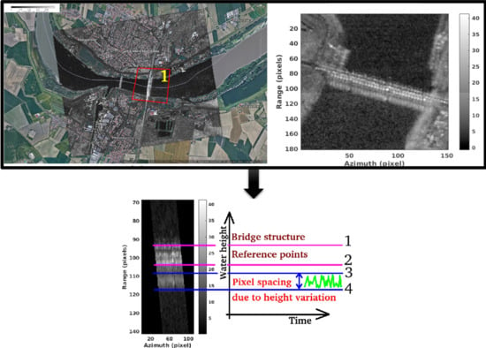
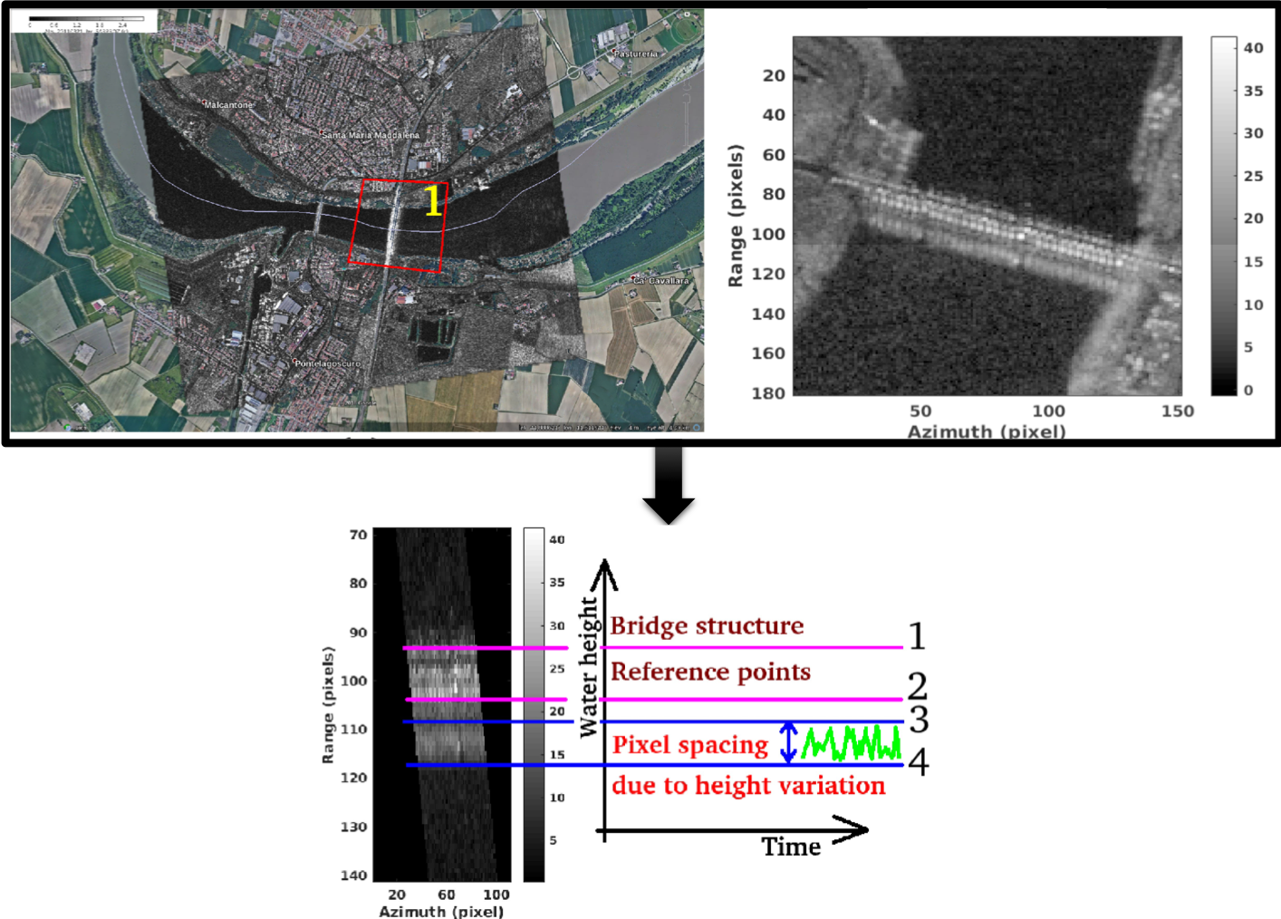
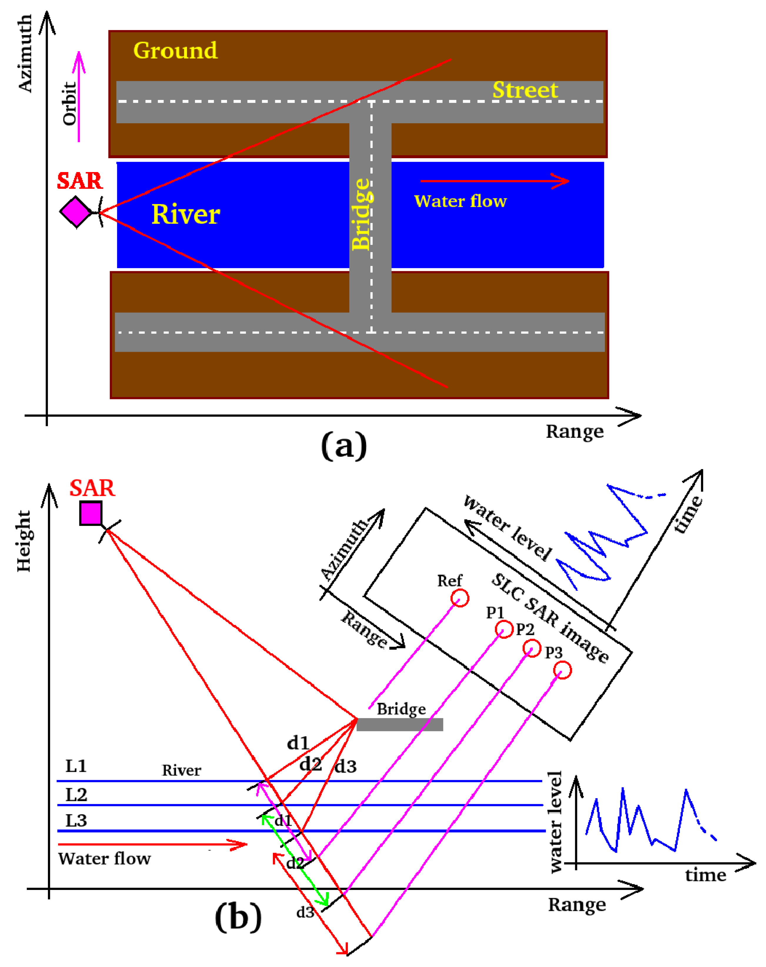
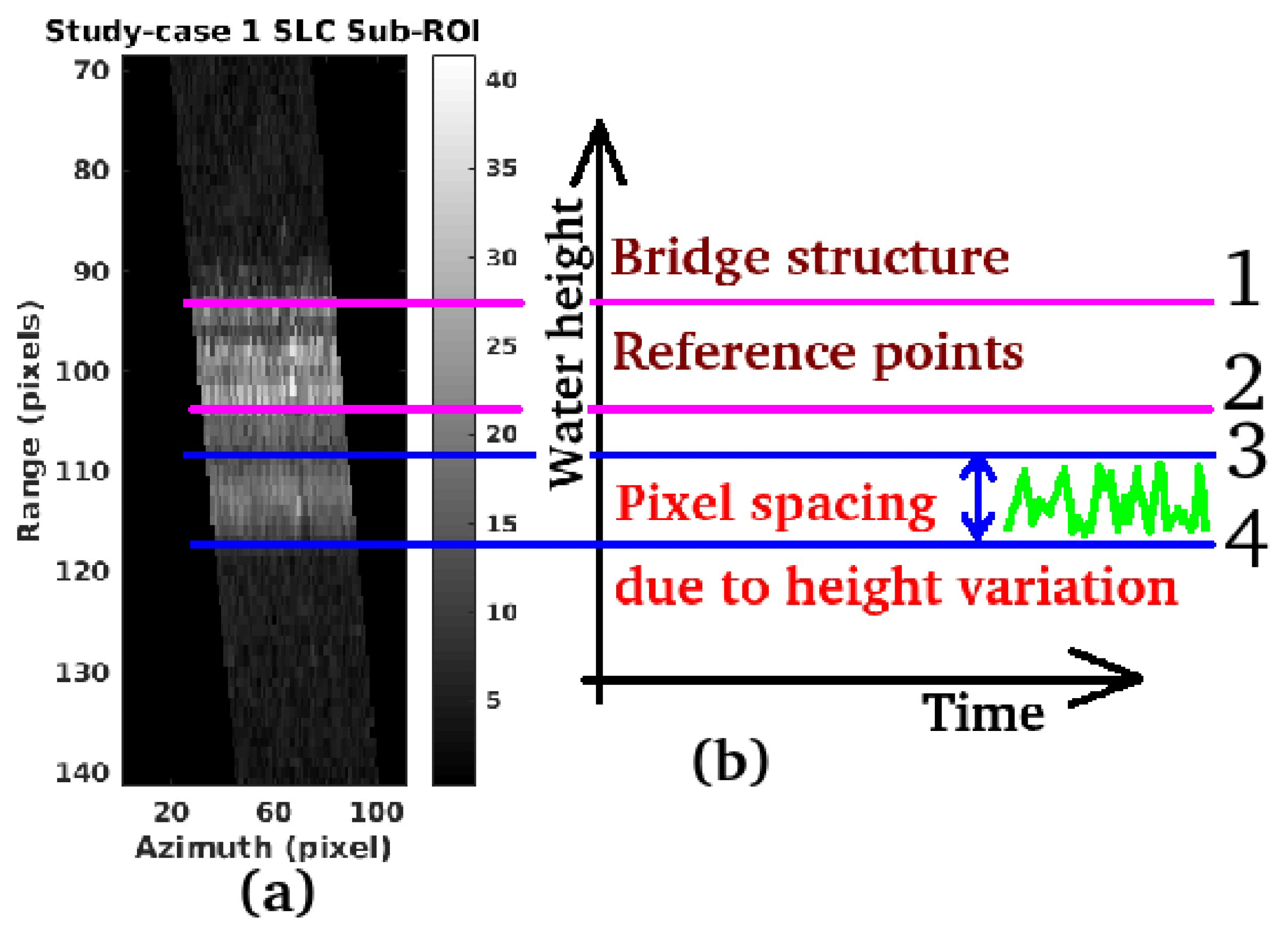
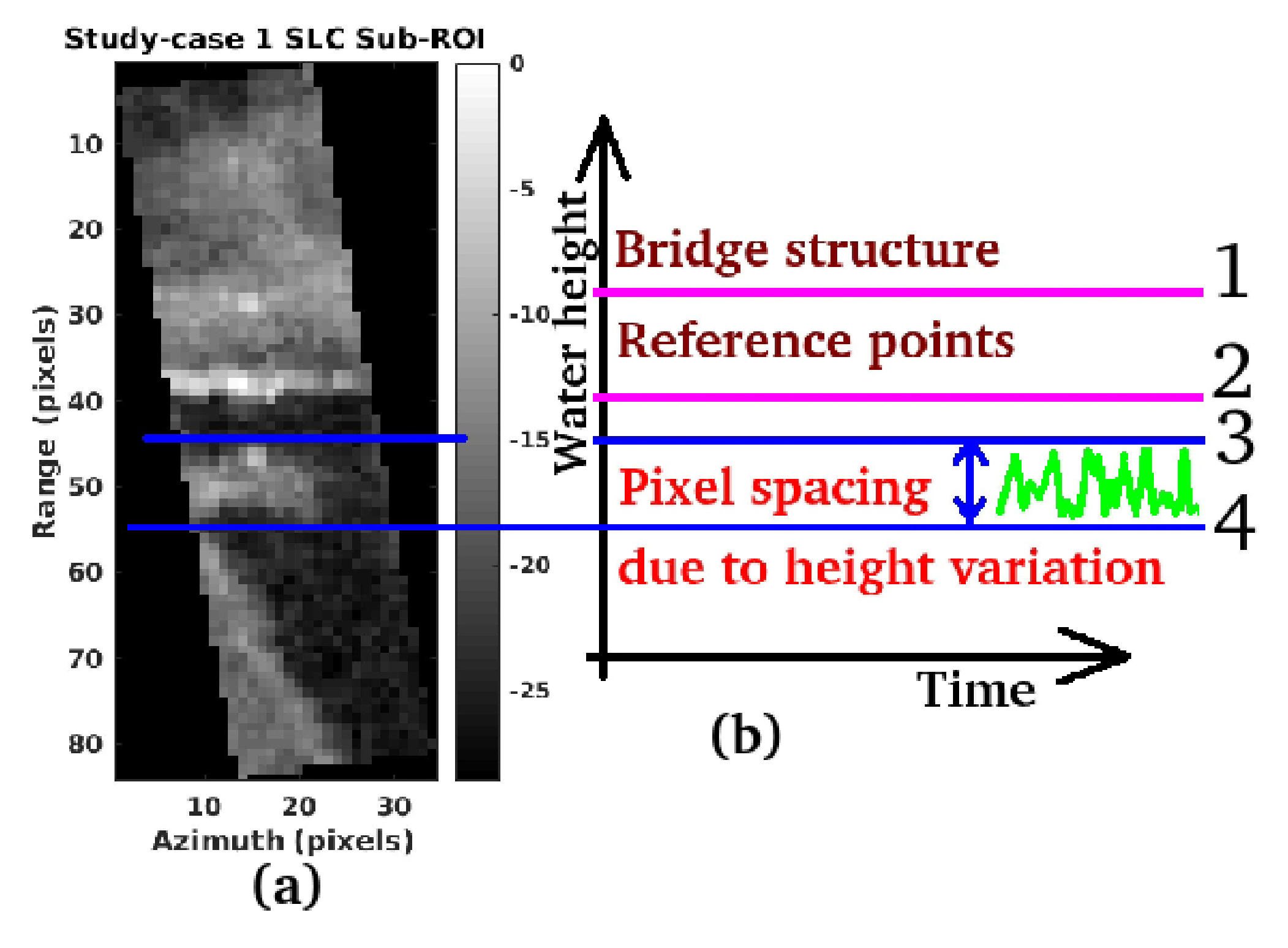
2.1. The Observation Geometry

The geometry of the proposed electromagnetic measurement system is depicted in Figure 1. Precisely, Figure 1a shows the scheme of an existing river on the SAR representation plane, in the range-azimuth reference system. The water of the river is represented flowing along the range direction and from left to right (this is represented by the red arrow visible on the right side of the figure). A bridge is present in the middle of the figure and crossing the azimuth dimension. Figure 1b represents what is shown in Figure 1a but in the height-range coordinates. It is clear that the Ref point, which is the focused single-bounce backscattered echo, is constituted by the front-edge of the bridge that is visible on the Single Look Complex (SLC) image. Its position is constant during the entire time series. The positions of points P1, P2 and P3 on the SLC projection screen, represents the double-bounce backscattered echoes of the same target. The distance of the two-way propagation system depends on the heights of the water levels L1, L2 and L3, which are variable with respect to the time.

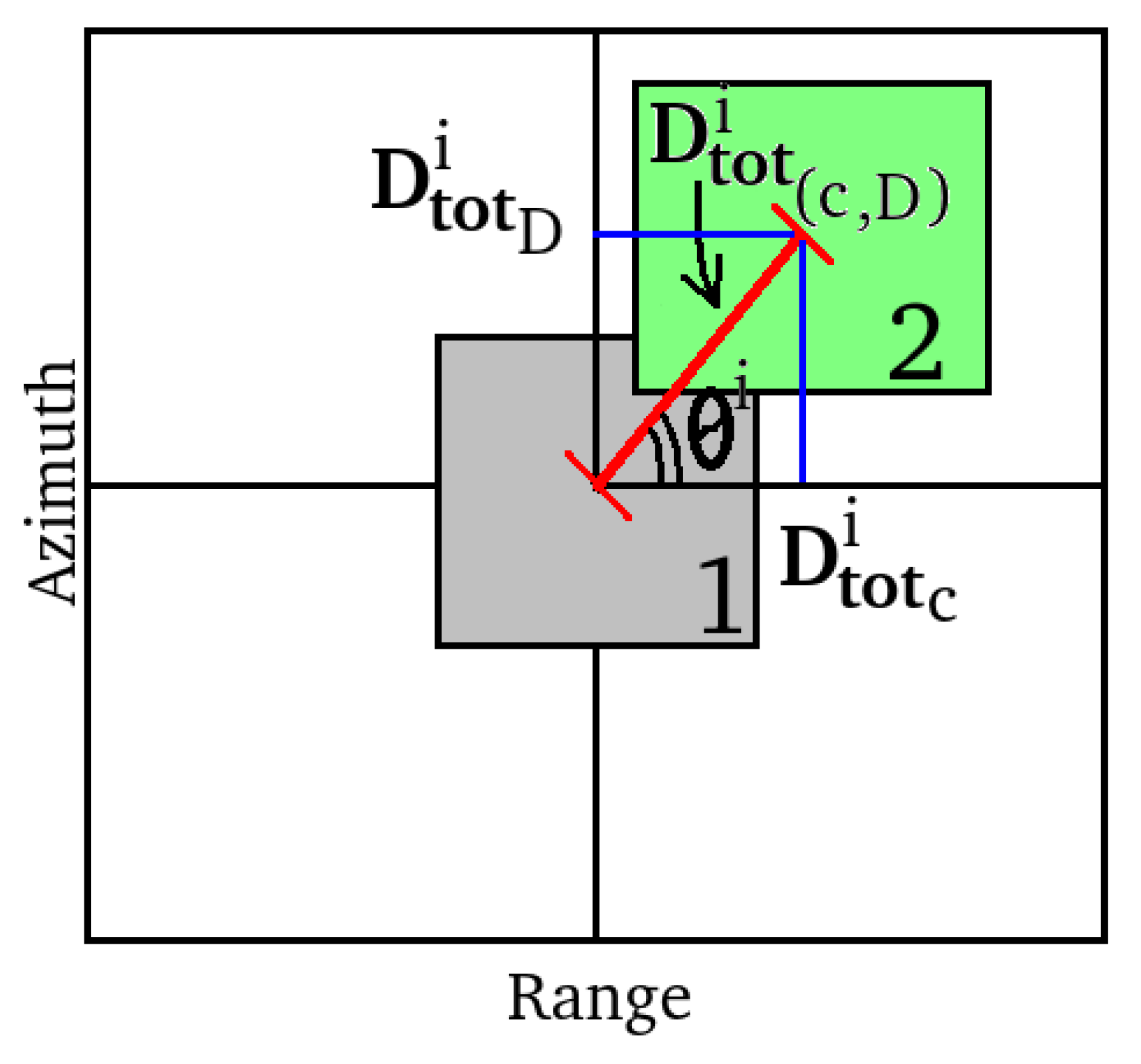
2.2. The Processing Scheme

The workflow of the proposed estimation technique is depicted in Figure 2 and comprises 5 main processing blocks. The main rationale of the proposed procedure is based on the pixel tracking. Sub-pixel offset tracking (SPOT) is a relevant technique to measure large-scale ground displacements in both range and azimuth directions. The technique is complementary to differential interferometric SAR and persistent scatterers interferometry when the radar phase information is unstable [23,24]. In this paper, we apply the SPOT in an alternative way, as explained in the following.
The starting point of this algorithm is a long temporal series of InSAR data but, instead of investigating the deformations of the ground, we investigated the movements of the double-bounce scattering effect of man made structures localized on the water surface. Although the variations in the water levels of rivers vary over time much faster with respect to the movements of the ground, we also apply the SPOT technique to trace their hydrometric levels. To this end, it is necessary to design a specific mathematical model that is described in detail below. Indeed, as shown in Figure 2, the starting point (block 1) is the selection of a long temporal series of SAR data, which is based on the desired temporal observation period. This series is, then, processed using images pairs in order to track the hydrometric levels variation over the time. Specifically, the magnitude at the output of the two-dimensional matched filter of the receiver chain can be expressed as the following matrix (for simplicity, we assume that target position in the range-azimuth plane is ( 0 , 0 ) ) [25] [Chapter 4], for each interferometric complex pair, indexed by i and belonging to a time series of length G:
r c , D i ( n c , n D ) = A sin ( n c δ R c / B c ) ( n c δ R c / B c ) × sin ( n D δ R D / B D ) ( n D δ R D / B D ) , i = 1 , , G n c = N c / 2 , , 0 , , N c / 2 , n D = N D / 2 , , 0 , , N D / 2 , N c , N D N ( even ) ,
where:
  • A is the backscattering coefficient;
  • N c is the number of pixels of the image along the range;
  • N D is the number of pixels of the image along the azimuth;
  • δ R c is the chirp resolution;
  • δ R D is the Doppler resolution;
  • n c is the chirp wavenumber;
  • n D is the Doppler wavenumber;
  • B c is the bandwidth of the transmitted chirp signal;
  • B D is the synthesized Doppler band.
Such data will necessarily have to be co-registered (the coregistration process consists of perfectly aligning the pixels of any slave image to the corresponding pixels of the master image. The alignment process is very precise and can also be accurately performed at the sub-pixel level). The co-registration stage is performed as the second stage of the processing chain. After co-registration, the stage 3 exploits the range shifts for an initial coarse estimation of the double-bounce shifts and error correction. To give a sketch of these steps, let consider the offset components of the sub-pixel normalized cross-correlation, that according to References [15,26] are described by the complex parameter D i tot ( c , D ) referred to as total displacement, which is given by:
D i tot ( c , D ) = D i displ ( c , D ) + D i topo ( c , D ) + D i orbit ( c , D ) + D i control ( c , D ) + D i atmosphere ( c , D ) + D i noise ( c , D ) , i = 1 , , G ,
where:
  • D i displ ( c , D ) is the offset component of the signal position presented in (1), generated by the variation of the river water level and detected as a sub-pixel misalignment existing between the first SAR image (master) and the i-th slave SAR image;
  • D topo ( c , D ) i is the offset component generated by the earth displacement when located on highly sloped terrain;
  • D orbit ( c , D ) i is the offset caused by residual errors of the satellite orbits;
  • D control ( c , D ) i is the offset component generated by general attitude and control errors of the flying satellite trajectory;
  • D atmosphere ( c , D ) i and D noise ( c , D ) i are the contributions accounting for change in the atmospheric and ionospheric dielectric constant and for decorrelation phenomena (spatial, temporal, thermal, etc.), respectively.
Note that the above equation accounts for the general case where displacement exists in both range and azimuth dimensions. In the operating scenario considered here, the displacement generated by the double-bounce scattering component of the bridge, when perturbed by the temporal variations of the river water levels, is significantly greater with respect to any other sporadic displacements due to physical phenomena. As depicted in Figure 1, this phenomenon is maximum when the longitudinal axis of the bridge is observed perpendicular to the range direction. With the above remarks in mind, we can assume that the contribution in the displacement D tot ( c , D ) i is greater along the range dimension. Thus, neglecting the azimuth component, we can consider D tot ( c , D ) i = D tot c i .
Figure 3 is a schematic representation of the parameters estimated by the coregistration procedure. The square number one is a focused pixel of the master image and the square number two is the same pixel but located on the slave image. The parameters D tot c i and θ i are the distance between the master and slave pixel centers and the angle respect to the horizontal axis respectively. In the present case, since the shift of the double-bounce scattering occurs in range, the parameter θ i = 0 so D tot D i = 0 . Moreover, the atmospheric time-variation during the very short acquisition time interval has little influence on the temporal component of the last displacement parameters because of its low accuracy. All errors are compensated for, choosing only high energy and stable points and subtracting the initial offsets in order to retrieve the shifts contributions only generated by the target displacement.
Once all the image pairs are co-registered and D tot c i is computed, we proceed with the estimation of the water level on a specific region of interest (ROI). The ROI extraction is performed by the block number 4 and the last computational block (number 5) performs a precise range shifts estimation and water level estimation as detailed in the sub-blocks (5.1–5.6). In particular, the data-input ROI are fed to the block 5.1 that extracts the sub-ROI, containing only the bridge. Processing stage number 5.2 performs the azimuth average of the sub-ROI and computational block 5.3 is designed to perform the pixel dilation by oversampling [21]. Computational block 5.4 performs the one-dimensional DFT (in the range direction) of the sub-ROI average. To this end, we compute
D F T ( r c , D i ( n c D tot c i , n D ) ) = R c , D i ( k c , k D ) exp j 2 π k c i N c i D tot c i ,
where
R c , D i ( k c , k D ) = D F T r c , D i ( n c , n D ) = n c = 0 N ˜ c 1 n D = 0 N ˜ D 1 A sin ( n c δ R c / B c ) sin ( n D δ R D / B D ) ( n c δ R c / B c ) ( n D δ R D / B D ) exp j 2 π k c N c n c exp j 2 π k D N D n D ,
with N ˜ c × N ˜ D the dimension of the sub-ROI under test and we have clearly exploited the shift theorem of the DFT.
The last two processing stages (blocks number 5.5 and 5.6) convert the phase variations from the output of the previous computational stage into effective water levels of the rivers. To this aim, let us observe that the term exp j 2 π k c N c ( D tot c i ) represents a rotational vector where the frequency is proportional to the temporal-space shift amount D tot c i . It follows that the higher the shift of the double-bounce pixel, the higher the oscillation frequency of the phasor. This frequency increasing will generate more turns of the phasor around the circle angle. All these turns, when unwrapped, represent a distance proportional to the height of the river water. As a phase unwrapping algorithm, we select the one-dimensional case of that developed in Reference [22]. Once the absolute phase value is estimated, it is suitably scaled through a constant factor obtained by comparing absolute phase measurement with the true height of the river. This operation is equivalent to an algorithm calibration procedure. Specifically, the river height at the i-th time instant is evaluated as follows (note that { R c , D i ( k c , k D ) } is known)
H w a t e r i = A c U n w r a p p exp j 2 π k N ( D tot c i ) , i = 1 , , G ,
where the term A c is the calibration parameter and the function U n w r a p p ( . ) performs the phase unwrapping algorithm described in Reference [22]. As for the the constant A c , it is obtained as
A c = H w a t e r 1 U n w r a p p exp j 2 π k c 1 N c 1 ( D tot c 1 ) .
where H w a t e r 1 is a measurement coming from fixed ground stations.
Finally, the computational stage number 5.5 performs the phase unwrapping of the frequency variation exponential term reported in (4) and (5) and the last stage number 5.6 estimates the integral below the unwrapped function.

3. Test on Simulated Data

The simulated data are generated in order to emulate as closely as possible the most suitable observation and geometry characteristics. The bridge is designed with a longitudinal axis perfectly perpendicular to the range direction, a bridge width of about 30 pixels and a maximum variation of double-bounce scattering of about 1.5 pixels. The radar is designed with the same features as the COSMO-SkyMed sensor.
In this specific case, simulated data consist of a sub-ROI reflectivity range profile for which the energy is shown in Figure 4a. From inspection of the figure, it is possible to notice the beginning and the end of the bridge edges. These scattering events, denoted by the numbers 1 and 2, are generated by the direct reflection events and they are directly projected onto the slant-range line. The energy peak generated by the double-bounce scattering mechanism is the one indicated by the number 3 and, thanks to the layover effect, is located behind the main scatterers. The position in time of peaks 1 and 2 remain stable over time because the bridge does not move while peak 3 changes its position due to the variation of the height level of the river’s water surface. According to the DFT property (6), a time-variation position of the peak number 3 is corresponding to a frequency variation of its DFT. The variation of the phasor oscillation frequency will increase its absolute phase value (unwrapped phase) [21]. This distance, appropriately scaled and then calibrated at the first observation performed by the ground station (terrain gauge), is being used as an indication of the river’s height. The input signal is represented by the sinusoidal sub-pixel variation indicated by arrow number 3. In Figure 4b), the unwrapped phases related to each interferometric pair are reported (the lines with different colors are corresponding to the different observations). The reconstructed level variation is depicted in Figure 4c. From Figure 4b we see that the output response of the function U n w r a p p ( . ) is linear so the parameter A c of Equation (5) represents the angular coefficient of the linear phases. The ripple in Figure 4c is present due to an oversampling factor of 10 has been used. The higher the oversampling factor, the less visible this noise will be. In the experimental data using the satellite sensor, a very high oversampling factor of 64 will be chosen.

4. Test on Cosmo-SkyMed Data

The performance of the procedure has been evaluated processing a long temporal series of CSK data using three different case studies which are described in detail in Section 4.1. The results estimated from satellite data are validated by comparison with the in-situ observations in Section 4.2.

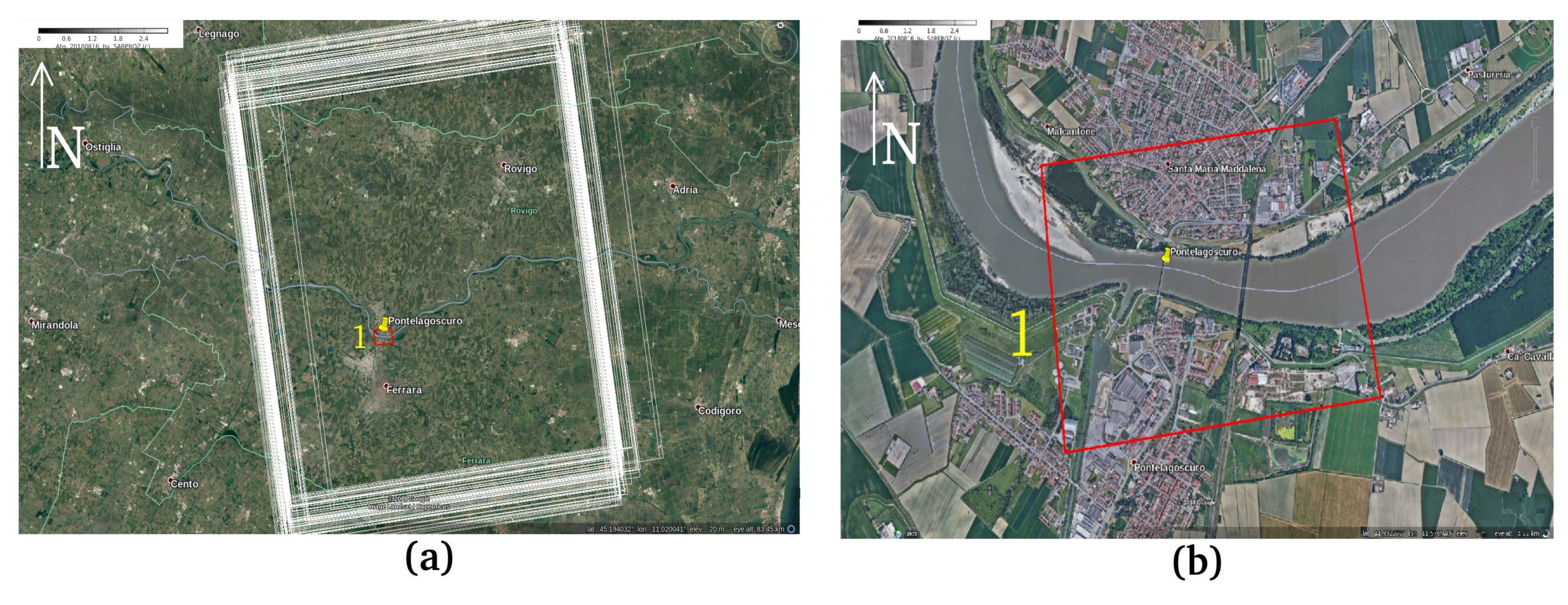
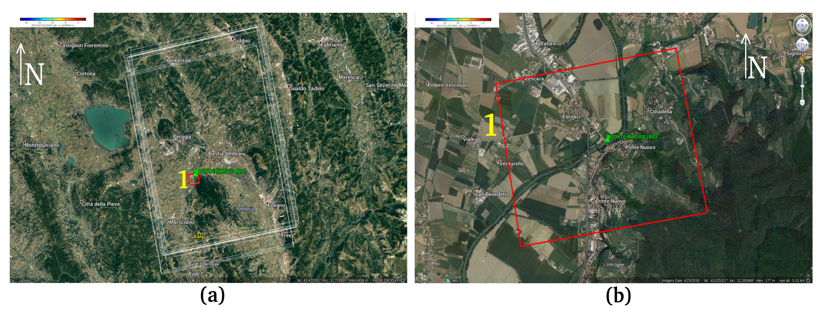
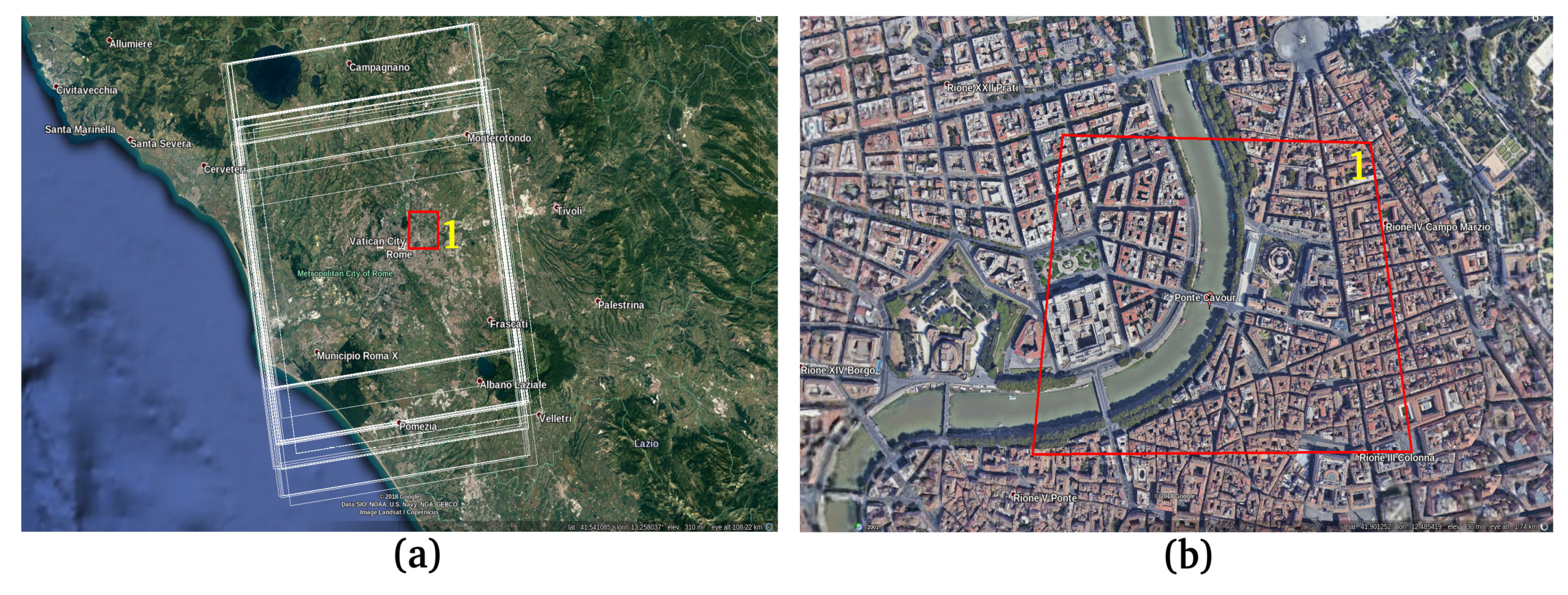
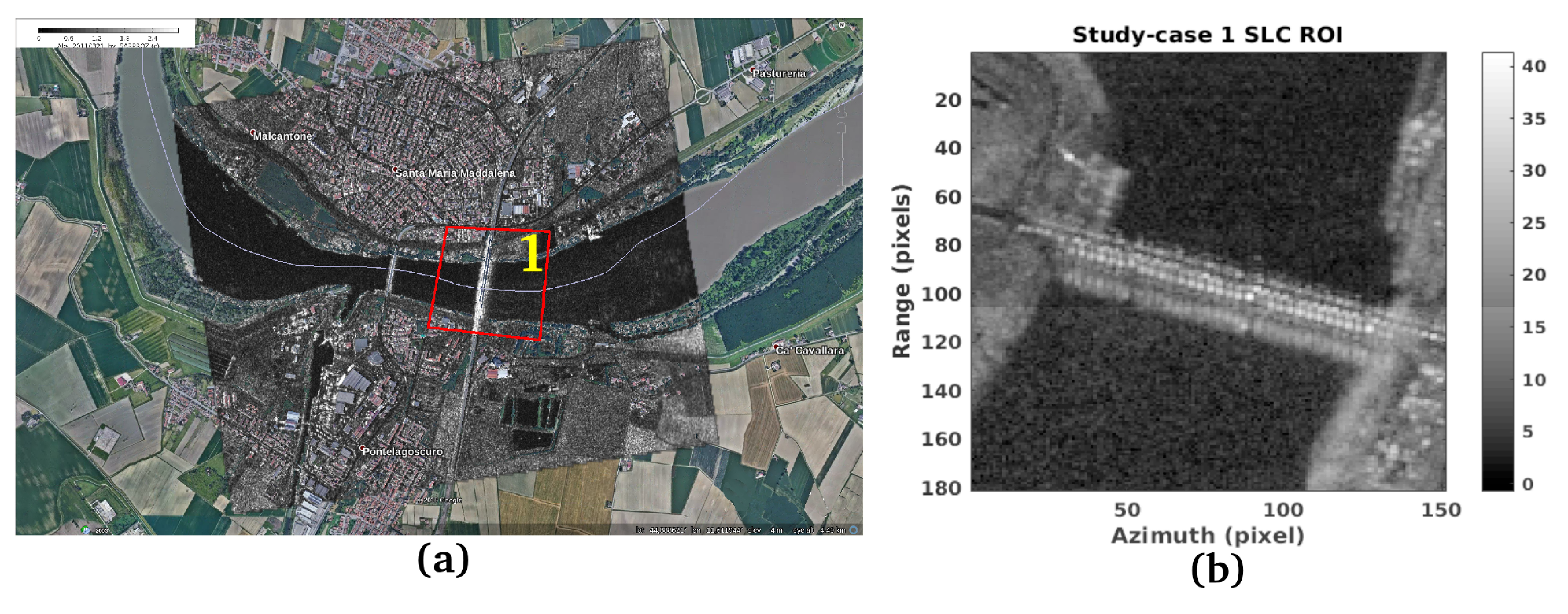
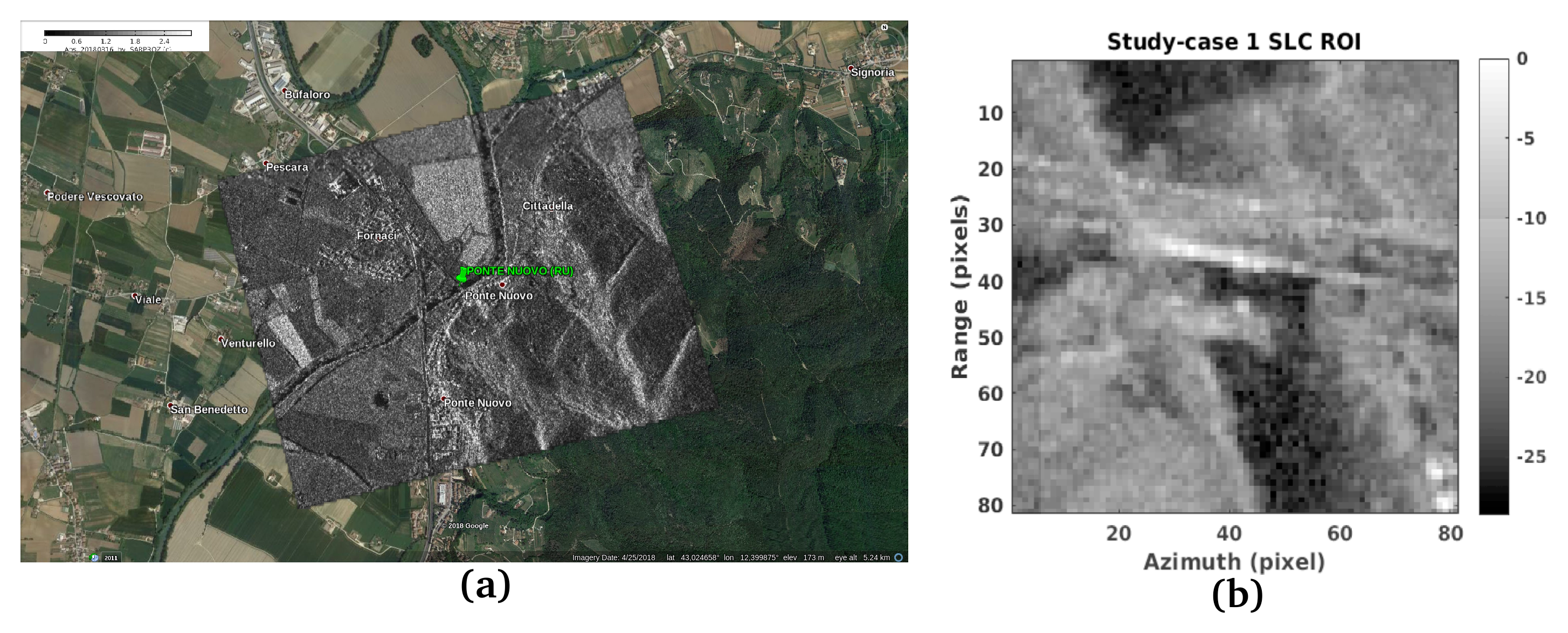
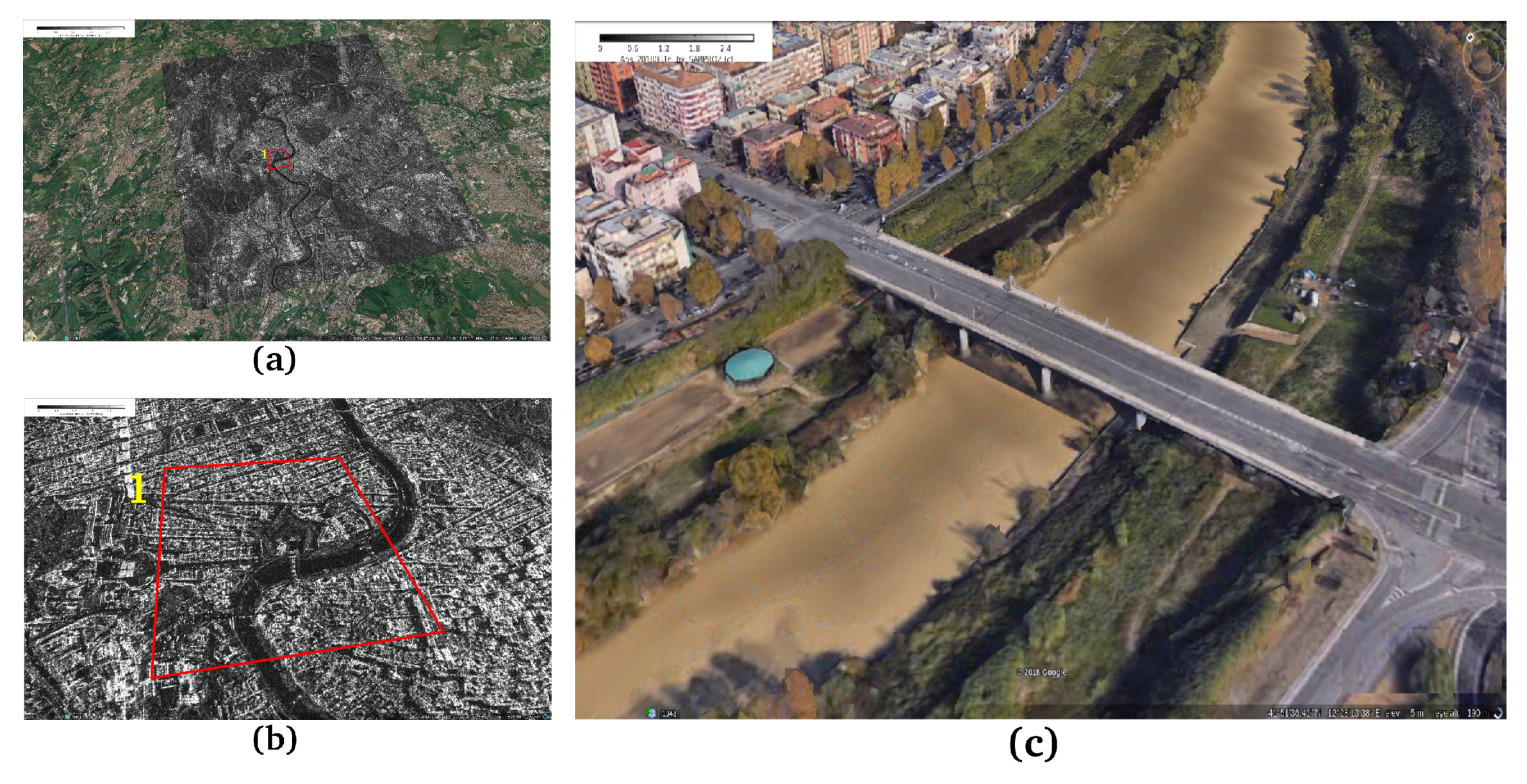
4.1. Case Studies and In-Situ Observations

The processed data belong to the persistent Earth observation mission called MAPITALY procured by the Italian Space Agency (ASI). This mission performs the interferometric observation of the whole Italian territory with a revisiting time of about 10 days. For the analysis, three datasets of CSK images were considered based on three study areas. The results estimated from satellite data were validated by comparison with the ground observations of water level recorded in a consistent period with respect to the satellite images. In particular, three gauged stations along two Italian rivers were considered—Pontelagoscuro along the Po River, Ponte Nuovo and Ripetta along the Tiber River.
The first case study observes the Po River located on the Northern Italy at the Pontelagoscuro station. Figure 5a shows the georeferenced representation of the SAR long temporal series. Inside the SAR acquisition footprints there is a small red box with a yellow marker inside, geolocated on the following coordinates: datum WGS-84 (EPSG): 4240, 44 53 16.66 N 11 36 29.42 E. This box is tagged in yellow with the number 1. This ROI-footprint is represented in detail in Figure 5b where the bridge is observed by an optical image and contoured by the same red box. The ground water levels are registered by the Agenzia Interregionale del Fiume Po.
The second data-set is measured over the Tiber river located in Central Italy. Figure 6a represents some footprints of the SAR observations. Inside the SAR acquisition footprints there is a small red box with a green marker inside, geolocated on the following coordinates—datum WGS-84 (EPSG): 4240, 43 00 37.84 N 12 25 44.89 E. This box is tagged in yellow with the number 1. This ROI-footprint is represented in detail in Figure 6b where the bridge is observed by an optical image and contoured by the same red box. The observed water levels are registered by the Servizio Idrografico of the Umbria Region.
The last case study is composed of satellite observations concentrated on the city of Rome. The optical representation of the environment where the river water level has been estimated is reported in Figure 7a. The picture also reports the footprints of the long temporal series of the interferometric SAR observations. The measurements are focused on the Cavour bridge where the optical representation of the infrastructure is reported in Figure 7b. The data are registered by the Agenzia Regionale Protezione Civile of the Lazio Region.
The number of processed images for study areas and the period of analysis is specified in Table 1. The number of images varies from 27 images for the study area at Rome and 106 for Pontelagoscuro station. The period of images is different, ranging from 2 to 9 years. For all the experiments, we set the cross-correlation window size to 128 × 128 pixels and the oversampling factor to 64 in both the range and azimuth directions. This value was found to be an optimal pixel dilation level. All the coregistration parameters are reported in Table 2.

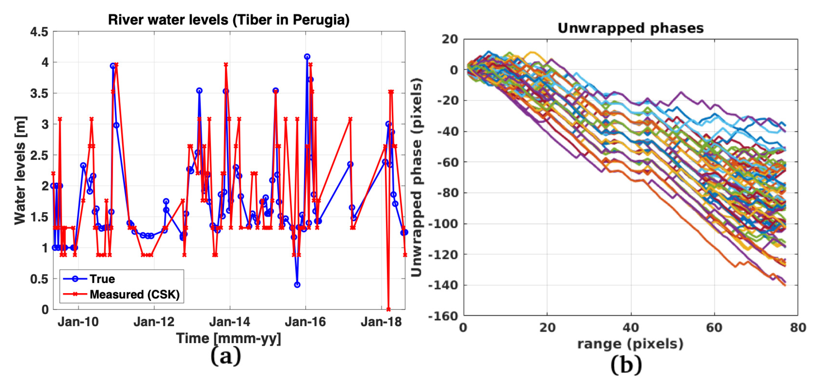
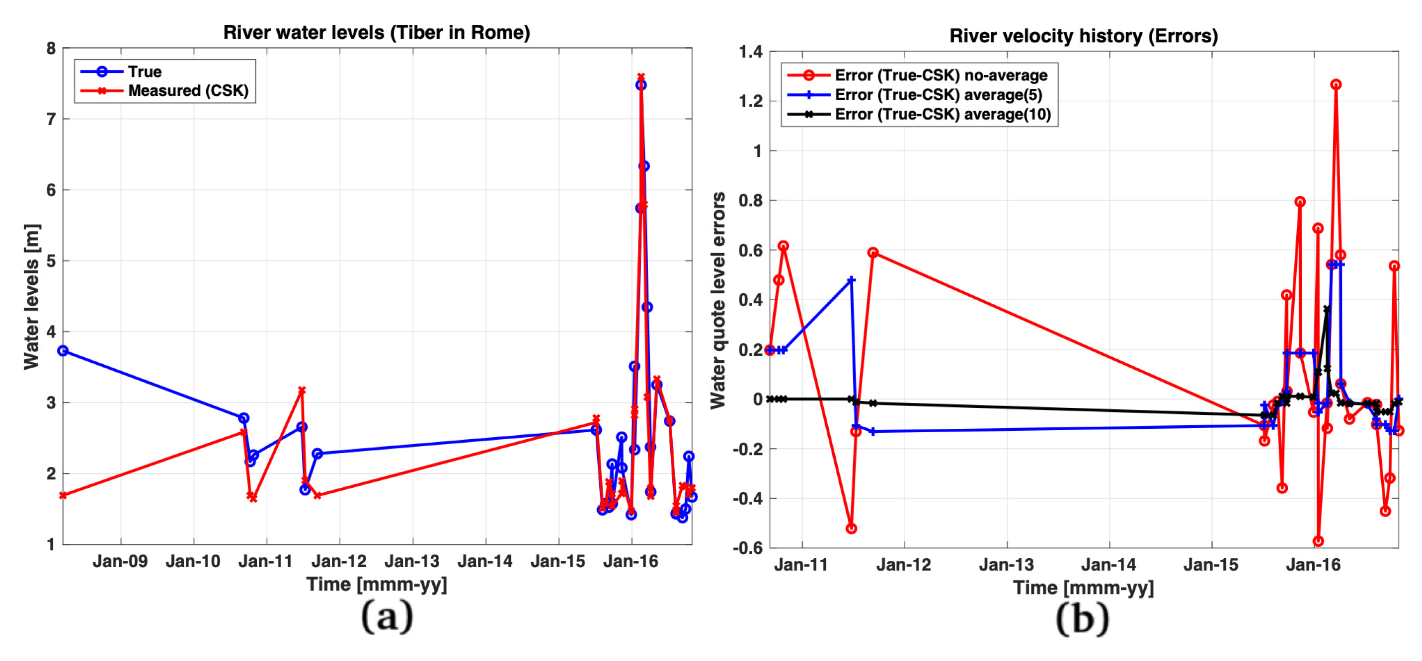
4.2. Experimental Results

In Figure 8a, the SLC-ROI is reported, referring to the small patch number 1 depicted in Figure 5a,b. This ROI contains the electromagnetic representation of the bridge, used to calculate the water levels of the Po river. The detailed sub-ROI SLC image is shown in Figure 8b. This sub-ROI consists of the data input of the computational block number 5 depicted by Figure 2. Figure 9a is the long temporal series time average sub-ROI particular. Figure 9b gives the description of the scattering events related to the bridge. The purple line number 1 represents the beginning of the bridge structure. Purple line 2 shows the position of the end of the bridge, this scattering event is considered to be a stationary landmark in time. The blue line 3 represents the lowest deviation of the double-bounce scattering event with respect to the reference point, which means that the river is in flood. Line 4 represents the slightest deviation of the double-bounce scattering event, if the pixel is represented it means that the river is dry. The variance of the double-bounce layovered backscattered echoes is strictly located inside the spatial gap contained by the blue layers 3 and 4. The temporal trend of this layover scattering line is a function of the river water level. The trend of the estimated water levels is depicted in Figure 10a. The blue line represents the water-levels measured by the CSK satellite system and the red function represents the ground truths given by the ground observation station. The unwrapped phases of the FT result are shown in Figure 10b.
Case study 2 has the objective of studying the trend of the Tiber heights in the part of the river that crosses the Umbrian region located in the Italian Central Apennines. This part of the Tiber is narrower with respect to the Po and the radar observations are a bit noisier. Considering this phenomenon, the estimation of the heights of the rivers on this section is more difficult. In Figure 11a the SLC-ROI is reported, referring to the small patch number 1 depicted in Figure 7a,b. This ROI contains the electromagnetic representation of the bridge, used to calculate the water levels of the Po river. The detailed sub-ROI SLC image is shown in Figure 11b. This sub-ROI consists of the data input of the computational block number 5 depicted by Figure 2. Figure 12a is the long temporal series time average sub-ROI particular. Figure 12b gives the description of the scattering events related to the bridge. The purple line number 1 represents the beginning of the bridge structure. Purple line 2 shows the position of the end of the bridge, this scattering event is considered to be a stationary landmark in time. The blue line 3 represents the lowest deviation of the double-bounce scattering event with respect to the reference point, which means that the river is in flood. Line 4 represents the slightest deviation of the double-bounce scattering event, if the pixel is represented it means that the river is dry. The variance of the double-bounce layovered backscattered echoes is strictly located inside the spatial gap contained by the blue layers 3 and 4. The temporal trend of this layover scattering line is a function of the river water level. The trend of the estimated water levels is depicted in Figure 13a. The blue line represents the water-levels measured by the CSK satellite system and the red function represents the ground truths given by the ground observation station. The unwrapped phases of the FT result are shown in Figure 13b.
In the final case, it was planned to quantify the water height levels of the Tiber River as it flows through the city center of Rome. Also for this case study the experimental measurements were compared with the ground-based measuring facilities. Figure 14a shows the georeferenced SAR extended image where the ROI is visible inside the red box tagged by the yellow number 1. The geolocated SAR ROI is represented in detail in Figure 14b where the bridge is observed and contoured by the same red box. Finally, the optical representation of the Cavour bridge is shown in Figure 14c. The double-bounce electromagnetic scattering effects were generated by the Cavour bridge (the yellow arrow which is geolocated on the following coordinates: datum WGS-84 (EPSG): 4240, 41 51 36.10 N 12 28 38.00 E). The temporal trend of the river water levels is depicted in Figure 15a. In Figure 15b, the errors corresponding to the estimated values in Figure 15a are reported. In addition to the errors represented by a red line, the errors of the estimated values averaged over 5 and 10 samples are shown with a blue and a black line, respectively. As expected, it could be convenient, in the case when the data are very noisy, to exploit the smoothing effect due to averaging. Moreover, from the non-averaged errors of Figure 15b, it can be seen that some measurements are wrong but such uncompliant samples are very few; in fact, observing the trend of the average errors on 5 and 10 samples a significant drop in the error can be seen, which remains well below one meter.

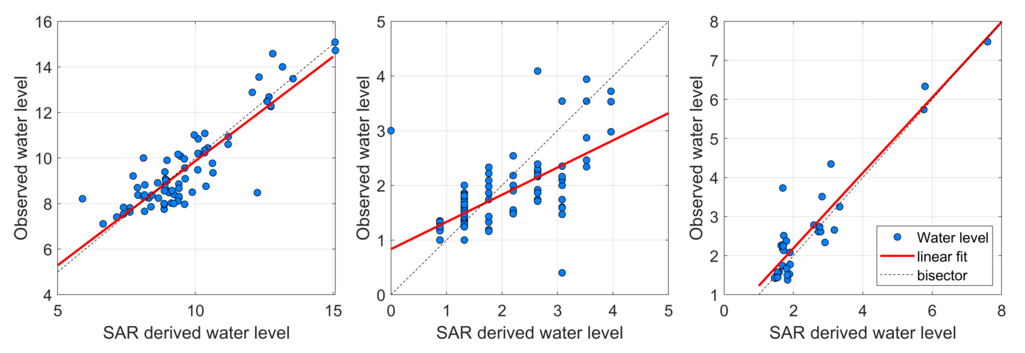
5. Discussion and Performance Assessment

This section provides comments on the experimental results observed in the three case studies. The experimental results show that the implemented algorithm is quite robust, although sometimes it fails to provide a reliable estimate. This is because there is a temporal misalignment from the actual SAR observation that occurs in Italy either early in the morning or late in the evening compared to the measurement of the instrument located in the immediate vicinity of the bridges. This time misalignment is also found to be many hours.
In Figure 16, the scatterplot is reported for each case study, representing the comparison between the water levels estimated by satellite and those observed by the in-situ station. For the Po and the Tiber in Rome (Figure 16 left and right) the water levels overlap the bisector line, as also indicated by the linear regression (red line). In the case of Tiber at Ponte Nuovo (Figure 16 center) the simulated water levels underestimate the ground-based observations up to 2 m, whereas they overestimate the higher water levels. Therefore, the red line does not lie upon the bisector line as the other two cases.
The worst performance are obtained for the Ponte Nuovo case study (as shown at the center of Figure 16). It is worth noticing that this case study has to be selected to provide an example of a difficult scene to analyze. This difficulty can be attributed to the width of the river that in this region is quite narrow (60 m as shown in Table 1) and is greatly contaminated by the surrounding vegetation. These characteristics can affect the satellite measurements and represent a good testbed for the proposed algorithm which, despite everything, would provide still reliable results as shown in the figure. A possible solution to improve the performance of the algorithm could be the installation of corner reflectors in the scene to mitigate the effect of the noise introduced in the radar measurements.
In order to quantify the performances of the analysis, four indicators are calculated:
  • the Pearsone correlation coefficient (R),
  • the Nash-Sutcliffe efficiency (NS) [27],
  • the root-mean square error (RMSE), expressed in [m],
  • the related root-mean square error (RRMSE), defined as the ratio between the RMSE and the mean of the observed water levels.
Table 3 shows the performances for the three case studies comparing the water levels estimated by the procedure and those observed by in-situ stations. As deduced by the scatterplots, best results are obtained for case study one and three, with coefficient of correlation greater than 0.88 and NS greater than 0.77.
Lower performances are obtained for case two with NS smaller than zero and RRMSE of 39%. However, if we calculate the performance considering the linear regression as shown in Figure 16 (center), the performances improve (NS = 0.43; RMSE = 0.51; RRMSE = 0.29). This means that the procedure can fail in terms of absolute values but can be a support to evaluate a variability of the water level if no other measurements are available, as for example in ungauged basins.
In the first case study, the value of the RMSE is quite high (0.91 m) comparing to the other two cases but the RRMSE is the lowest. This is due to the fact that the RMSE is an absolute figure of merit that is not related to a specific value as, on the contrary, the RRMSE. In fact, for the case 1, the water levels range from 6 to 15 m, whereas a narrower range characterizes the other two cases.

6. Conclusions

In this paper, an innovative procedure for estimating the water flow elevation of rivers is proposed. Today, a shared and worldwide database containing historical and reliable data concerning the water surface elevation of rivers has not been completed. Many areas are still unmonitored and due to the large importance of fresh water, an evaluation of the river system is fundamental. The main scope of this research is contributing to solving this information-gap problem by designing a SAR signal processing technique having the capability to perform water flow level estimation. The problem of measuring such data is usually solved by designing an ATI SAR geometry, which is constituted by two radars spatially distanced by a baseline extended in the azimuth direction. In the case of space-borne missions the performing of ATI can be an unusual and difficult task. For several single-antenna spaceborne SAR satellite systems, the refocusing of ATI observations from one raw data is a problem because of the not-oversampled nature of the received electromagnetic bursts. This phenomenon makes raw data very similar to a white random process and appearing interlaced Doppler bands completely disjoint. After the range-Doppler focusing process, this problem causes decorrelation when observing the ATI phase of distributed targets. Spaceborne LOS level measurements could be taken into consideration only for small and very coherent targets and in any case were located within the same radar resolution cell. This paper proposed the application of a robust technique for tracking the double-bounce reflections of some principal bridges crossing the rivers and to measure the gap space existing between the river surface and the bridges. The developed algorithm tracked over time the double-bounce scattering event position reflected on the river surface with respect to the single-bounce and direct backscattered echoes form the principal structures of the bridge. River water-flow data were indirectly retrieved by converting the time-domain water surface variation in velocities. The experiments were evaluated by processing simulated and a long temporal series of COSMO-SkyMed data.

Author Contributions

Conceptualization, F.B., A.T., P.A., C.C. and D.O.; Data curation, F.B. and A.T.; Formal analysis, F.B., A.T., P.A., C.C. and D.O.; Funding acquisition, F.B.; Investigation, F.B., A.T., P.A., C.C. and D.O.; Methodology, F.B., A.T., P.A., C.C. and D.O.; Resources, F.B., A.T., P.A. and C.C.; Software, F.B.; Supervision, F.B. and D.O.; Validation, F.B. and D.O.; Visualization, F.B.; Writing original draft, F.B. and D.O.; Writing review & editing, F.B., A.T., P.A., C.C. and D.O.

Funding

This research received no external funding.

Conflicts of Interest

The authors declare no conflict of interest.

References

  1. McGraw-Hill Book Company. Open Channel Hydraulics, Ven Te Chow, 1959: Open Channel Hydraulics; Open Channel Hydraulics, Kogakusha: Tokyo, Japan, 1959. [Google Scholar]
  2. Hannah, D.M.; Demuth, S.; van Lanen, H.A.J.; Looser, U.; Prudhomme, C.; Rees, G.; Stahl, K.; Tallaksen, L.M. Large-scale river flow archives: Importance, current status and future needs. Hydrol. Process. 2011, 25, 1191–1200. [Google Scholar] [CrossRef]
  3. Smith, L.C. Satellite remote sensing of river inundation area, stage, and discharge: A review. Hydrol. Process. 1997, 11, 1427–1439. [Google Scholar] [CrossRef]
  4. Bjerklie, D.M.; Dingman, S.L.; Vorosmarty, C.J.; Bolster, C.H.; Congalton, R.G. Evaluating the potential for measuring river discharge from space. J. Hydrol. 2003, 278, 17–38. [Google Scholar] [CrossRef]
  5. Bjerklie, D.M.; Moller, D.; Smith, L.C.; Dingman, S.L. Estimating discharge in rivers using remotely sensed hydraulic information. J. Hydrol. 2005, 309, 191–209. [Google Scholar] [CrossRef]
  6. Bjerklie, D.M. Estimating the bankfull velocity and discharge for rivers using remotely sensed river morphology information. J. Hydrol. 2007, 341, 144–155. [Google Scholar] [CrossRef]
  7. Koblinsky, C.J.; Clarke, R.T.; Brenner, A.C.; Frey, H. Measurement of River Level Variations with Satellite Altimetry. Water Resour. Res. 1993, 29, 1839–1848. [Google Scholar] [CrossRef]
  8. Biancamaria, S.; Frappart, F.; Leleu, A.S.; Marieu, V.; Blumstein, D.; Desjonquères, J.D.; Boy, F.; Sottolichio, A.; Valle-Levinson, A. Satellite radar altimetry water elevations performance over a 200 m wide river: Evaluation over the Garonne River. Adv. Space Res. 2016, 59, 128–146. [Google Scholar] [CrossRef]
  9. Normandin, C.; Frappart, F.; Diepkilé, A.T.; Marieu, V.; Mougin, E.; Blarel, F.; Lubac, B.; Nadine, B.; Abdramane, B. Evolution of the Performances of Radar Altimetry Missions from ERS-2 to Sentinel-3A over the Inner Niger Delta. Remote Sens. 2018, 10, 833. [Google Scholar] [CrossRef]
  10. Schneider, R.; Tarpanelli, A.; Nielsen, K.; Madsen, H.; Bauer-Gottwein, P. Evaluation of multi-mode Cryosat-2 altimetry data over the Po River against in situ data and a hydrodynamic model. Adv. Water Resour. 2018, 112, 17–26. [Google Scholar] [CrossRef]
  11. Fu, L.L.; Alsdorf, D.; Rodríguez, E.; Morrow, R.; Mognard, N.; Lambin, J.; Vaze, P.; Lafon, T. The SWOT (Surface Water and Ocean Topography) Mission: Spaceborne Radar Interferometry for Oceanographic and Hydrological Applications. In Proceedings of the OceanObs’09: Sustained Ocean Observations and Information for Society, Venice, Italy, 21–25 September 2009; Hall, J., Harrison, D.E., Stammer, D., Eds.; ESA Publication WPP-306: New York, NY, USA, 2009; Volume 2. [Google Scholar]
  12. Matgen, P.; Schumann, G.; Henry, J.B.; Hoffmann, L.; Pfister, L. Integration of SAR-derived river inundation areas, high-precision topographic data and a river flow model toward near real-time management. Int. J. Appl. Earth Obs. Geoinf. 2007, 9, 247–263. [Google Scholar] [CrossRef]
  13. Goldstein, R.M.; Richard, M.; Zebker, H.A. Interferometric radar measurement of ocean surface currents. Nature 1987, 328, 707–709. [Google Scholar] [CrossRef]
  14. Romeiser, R.; Breit, H.; Eineder, M.; Runge, H.; Flament, P.; De Jong, K.; Vogelzang, J. Current measurements by SAR along-track interferometry from a Space Shuttle. IEEE Trans. Geosci. Remote Sens. 2005, 43, 2315–2324. [Google Scholar] [CrossRef]
  15. Nitti, D.O.; Hanssen, R.F.; Refice, A.; Bovenga, F.; Nutricato, R. Impact of DEM-assisted coregistration on high-resolution SAR interferometry. IEEE Trans. Geosci. Remote Sens. 2011, 49, 1127–1143. [Google Scholar] [CrossRef]
  16. Michel, R.; Avouac, J.P.; Taboury, J. Measuring ground displacements from SAR amplitude images: Application to the Landers earthquake. Geophys. Res. Lett. 1999, 26, 875–878. [Google Scholar] [CrossRef]
  17. Strozzi, T.; Luckman, A.; Murray, T.; Wegmuller, U.; Werner, C.L. Glacier motion estimation using SAR offset-tracking procedures. IEEE Trans. Geosci. Remote Sens. 2002, 40, 2384–2391. [Google Scholar] [CrossRef] [Green Version]
  18. Casu, F.; Manconi, A. Four-dimensional surface evolution of active rifting from spaceborne SAR data. Geosphere 2016, 12, 697–705. [Google Scholar] [CrossRef] [Green Version]
  19. Biondi, F. COSMO-SkyMed Staring Spotlight SAR Data for Micro-Motion and Inclination Angle Estimation of Ships by Pixel Tracking and Convex Optimization. Remote Sens. 2019, 11, 766. [Google Scholar] [Green Version]
  20. Biondi, F.; Addabbo, P.; Clemente, C.; Orlando, D. Micro-Motion Estimation of Maritime Targets Using Pixel Tracking in Cosmo-Skymed Synthetic Aperture Radar Data: An Operative Assessment. Remote Sens. 2019, 11, 1637. [Google Scholar] [CrossRef]
  21. Oetken, G.; Parks, T.W.; Schussler, H. New results in the design of digital interpolators. IEEE Trans. Acoust. Speech Signal Process. 1975, 23, 301–309. [Google Scholar] [CrossRef]
  22. Goldstein, R.M.; Zebker, H.A.; Werner, C.L. Satellite radar interferometry: Two-dimensional phase unwrapping. Radio Sci. 1988, 23, 713–720. [Google Scholar] [CrossRef] [Green Version]
  23. Wang, Z.; Perissin, D.; Lin, H. Subway tunnels identification through Cosmo-SkyMed PSInSAR analysis in Shanghai. In Proceedings of the 2011 IEEE International Geoscience and Remote Sensing Symposium, Vancouver, BC, Canada, 24–29 July 2011. [Google Scholar]
  24. Ullo, S.L.; Addabbo, P.; Di Martire, D.; Sica, S.; Fiscante, N.; Cicala, L.; Angelino, C.V. Application of DInSAR Technique to High Coherence Sentinel-1 Images for Dam Monitoring and Result Validation Through In Situ Measurements. IEEE J. Sel. Top. Appl. Earth Obs. Remote Sens. 2019, 12, 875–890. [Google Scholar] [CrossRef]
  25. Richards, M.A. Fundamentals of Radar Signal Processing; Tata McGraw-Hill Education: New York, NY, USA, 2005. [Google Scholar]
  26. Biondi, F.; Clemente, C.; Orlando, D. An atmospheric phase screen estimation strategy based on multi-chromatic analysis for differential interferometric synthetic aperture radar. IEEE Trans. Geosci. Remote Sens. 2019. [Google Scholar] [CrossRef]
  27. Nash, J.; Sutcliffe, J. River flow forecasting through conceptual models part I—A discussion of principles. J. Hydrol. 1970, 10, 282–290. [Google Scholar] [CrossRef]
Figure 1. Observation geometry for the river water flow elevation estimation: (a) Range-azimuth representation (b); Range-height representation.
Remotesensing 11 02574 g001
Figure 2. Flow chart of the main procedure to extract water level information from a temporal series of synthetic aperture radar (SAR) data.
Remotesensing 11 02574 g002
Figure 3. Schematic representation of isolated pixels with a certain shift due to space displacement.
Remotesensing 11 02574 g003
Figure 4. Results of simulated data. (a): reflectivity profile. (b): Unwrapped phases. (c): water-levels estimated results (pixels).
Remotesensing 11 02574 g004
Figure 5. Case study 1 optical representations. (a): georeferenced footprints of the SAR long temporal series. (b): region of interest (ROI) footprint.
Remotesensing 11 02574 g005
Figure 6. Case study 2 optical representations. (a): georeferenced footprints of the SAR long temporal series. (b): ROI footprint.
Remotesensing 11 02574 g006
Figure 7. Case study 3 optical representations. (a): georeferenced footprints of the SAR long temporal series. (b): ROI footprint.
Remotesensing 11 02574 g007
Figure 8. Case study 1 magnitude SAR images. (a): Geolocated image with ROI footprint representation. (b) Particular of the ROI magnitude in the slant coordinates.
Remotesensing 11 02574 g008
Figure 9. Case study 1 Sub-ROI parameters. (a): Sub-ROI SAR image representation in the slant coordinates. (b): Scattering parameters on the reference points and pixel spacing trend.
Remotesensing 11 02574 g009
Figure 10. Case study 1 experimental measurements. (a): Water levels observed by the ground measurement station (blue line) and by the satellite (red line). (b): Unwrapped phases.
Remotesensing 11 02574 g010
Figure 11. Case study 2 magnitude SAR images. (a): Geolocated image with ROI footprint representation. (b) Particular of the ROI magnitude in the slant coordinates.
Remotesensing 11 02574 g011
Figure 12. Case study 2 Sub-ROI parameters. (a): Sub-ROI SAR image representation in the slant coordinates. (b): Scattering parameters on the reference points and pixel spacing trend.
Remotesensing 11 02574 g012
Figure 13. Case study 2 experimental measurements. (a): Water levels observed by the ground measurement station (blue line) and by the satellite (red line). (b): Unwrapped phases.
Remotesensing 11 02574 g013
Figure 14. (a): Case study 3 ROI. (b): ROI footprint. (c): Cavour bridge optical image.
Remotesensing 11 02574 g014
Figure 15. Case study 3 results. (a): Ground-station data (red) and satellite observations (blue), versus pixels. (b): Water level errors versus time. Blue: CSK versus true. Red: CSK versus true (5 observations average). Black: CSK versus true (10 observations average).
Remotesensing 11 02574 g015
Figure 16. Scatterplot of the water levels estimated by satellite and observed by in-situ stations for Po at Pontelagoscuro (left), Tiber at Ponte Nuovo (center) and Tiber at Ripetta (right).
Remotesensing 11 02574 g016
Table 1. Satellite datasets used in the analysis and corresponding river gauged stations
STATIONRIVERCOORDINATES (WGS-84)Time of Obs.Images
Number
River Width
[m]
PontelagoscuroPo44 53 18.84 N, 11 36 28.89 EMay 2009–Aug. 2018106340
Ponte NuovoTiber43 00′37.11 N, 12 25 45.15 EMar. 2011–Apr. 20177660
RipettaTiber41 54 17.59 N 12 28 27.84 ESept. 2009–Oct. 201637100
Table 2. Coregistration parameters
ParameterValue
Initial shiftsCoarse cross-correlation
Number of points4000
Correlation threshold0.8
Oversampling factor200
search pixel window48x48 pixel
Points skimming (minimum points)30
Use of DEMYes
Doppler Centr. Est. StrategyPolynomials
Table 3. Performance indicators of the simulated water levels versus the ground-based observations.
STATIONRNSRMSE [m]RRMSE
Pontelagoscuro0.880.770.910.10
Ponte Nuovo0.65−0.030.680.39
Ripetta0.930.850.550.21

