1. Introduction
Nowadays, position information has become key information in people’s daily lives. This has inspired position-based services, which aim to provide personalized services to mobile users whose positions are changing [
1]. Therefore, obtaining a precise position is a prerequisite for these services. The most commonly used positioning method in the outdoor environment is the Global Navigation Satellite System (GNSS). In most cases, however, people spend more than 70% of their time indoors [
2]. Therefore, accurate indoor positioning has important practical significance. Although GNSS is a good choice for outdoor positioning, due to signal occlusion and attenuations, it is often useless in indoor environments. Thus, positioning people accurately in indoor scenes remains a challenge and it has stimulated a large number of indoor-positioning methods in recent years [
3]. Among these methods, fingerprint-based algorithms are widely used. Their fingerprint databases include Wi-Fi [
4,
5,
6,
7,
8], Bluetooth [
9,
10], and magnetic field strengths [
11,
12]. Although these methods are easy to implement, construction of a fingerprint database is usually labor-intensive and time-consuming. Moreover, it is difficult for their results to meet the needs of high-accuracy indoor positioning.
Given that humans use their eyes to see where they are, mobile platforms can also do this with cameras. A number of visual positioning methods have been proposed in recent years. These positioning methods are divided into three categories: image retrieval based methods, visual landmarks-based methods, and learning-based methods.
Image retrieval based methods treat the positioning task as an image retrieval or recognition process [
13,
14,
15]. They usually have a database that are augmented with geospatial information, and every image in the database is described through the same specific features. These methods perform a first step to retrieve candidate images from the database according to a similarity search, and the coarse position information of the query image is then obtained based on the geospatial information of these candidate images. So the first step, similar image retrieval process, is critical. The brute-force approach, which is a distance comparison between feature descriptor vectors, is often used for similarity search. Some positioning methods based on feature descriptors [
16,
17,
18] adopt brute-force comparison for the similarity search process of image retrieval. However, it is computationally intensive when the images of a database are described with high-dimensional features, limiting its scope of applications. Azzi et al. [
19] use a global feature-based system to reduce the search space and find candidate images in the database, then the local feature scale-invariant feature transform (SIFT) [
20] is adopted for points matching in pose estimation. Some researchers try to trade accuracy for rapidity by using approximate nearest neighbor search, such as quantization [
21] and vocabulary tree [
22]. Another common way to save time and memory of similarity search is principal component analysis (PCA), which has been used to reduce the size of feature vectors and descriptors [
23,
24]. Some works use correlation algorithms, such as sum of absolute difference (SAD), for computing similarity between query image and database images [
25,
26]. In recent studies, deep learning-based algorithms are an alternative to aforementioned methods. Razavian et al. [
27] use features extracted from a network as an image representation for image retrieval in a diverse set of datasets. Yandex et al. [
28] propose a method that aggregates local deep features to product descriptors for image retrieval. After a set of candidate images are retrieved, the position information of the query image is calculated according to the geospatial information of these candidate images through a weighting scheme or linear combination. However, because this position result is not calculated by strict geometric relations, it is rough in most cases and difficult to meet the requirement of high-accuracy positioning.
Visual landmarks-based positioning methods aim to provide a six degrees of freedom (DoF) pose of the query image. Generally, visual landmarks in the indoor environments includes natural landmarks and artificial landmarks. The natural landmarks refer to the geo-tagged 3D database, which is represented by feature descriptors or images with poses. This database could have been built thanks to the mapping module of simultaneous localization and mapping (SLAM) [
29,
30]. Then the pose of query image is estimated by means of re-localization module and feature correspondence [
31,
32,
33,
34,
35]. Although the results of these methods are of good accuracy, it takes a long time to match the features of query image with geo-tagged 3D database, especially when the indoor scenes are large. In addition to natural landmarks, there are also positioning methods based on artificial landmarks, e.g., Degol et al. [
36] proposed a fiducial marker and detection algorithm. In reference [
37], the authors proposed a method to simultaneously solve the problems of positioning from a set of squared planar markers. However, positioning from a planar marker suffers from the ambiguity problem [
38]. Since these methods require posting markers in the environments, they are not suitable for places such as shopping malls that maintain a clean appearance.
In addition to the traditional visual-positioning method based on strict geometric relations, with the rapid development of deep learning in recent years scholars have proposed many learning based visual-positioning methods [
39,
40,
41]. The process of these methods are broken down into two steps: model training and pose prediction. They train models through given images with known pose information, and the indoor environments are expressed as the trained models. The pose of a query image is then regressed through the trained models. Some methods even learn the pose directly [
42,
43]. These methods, which are based entirely on learning, have better performance in weak-textured indoor scenes, but are less accurate or have lower generalization ability to large indoor environments than traditional visual-positioning methods [
44]. Therefore, some methods use trained models to replace modules of traditional visual-positioning methods, such as depth estimation [
45,
46,
47], loop detection [
48], and re-localization [
49]. The method proposed by Chen et al. [
50] uses a pre-trained network for image recognition. It retrieves two geo-tagged red-green-blue (RGB) images from database, and then use traditional visual positioning method for pose estimation. This method performs well on public dataset, but its database images are hand-picked, which increases the workload of database construction. Moreover, the two retrieved geo-tagged RGB images should have favorable geometric configuration (e.g., sufficient intersection angle) for high-accuracy depth estimation. However, this favorable configuration is not guaranteed by the existing two-image methods. This is a potential disadvantage of these methods. Our RGB-D database method directly provides high accuracy depth information from only one image, this not only ensures high accuracy of positioning, but also improves the efficiency of image retrieval.
To overcome the limitations of the aforementioned methods, in this paper, a high-accuracy indoor visual-positioning method with automated RGB-D image database construction is presented. Firstly, we propose an automated database construction process, making the constructed database more objective than a hand-picked database and thus reducing the workload. The database is automatically constructed according to the rules, which reduces the redundancy of database and improves the efficiency of the image-retrieval process. Secondly, considering the requirement of real-time positioning, we introduce a convolutional neural network (CNN) model for a robust and efficient retrieving candidate images. Thirdly, different from aforementioned image retrieval based positioning methods, we replace rough combination of geospatial information with strict geometric relations to calculate the position of query image for high-accuracy positioning. Finally and most importantly, by combining the above three components into a complete indoor-positioning method, we obtain high-accuracy results in an indoor environment and the whole process is time efficient.
2. Methodology
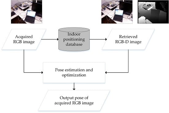
In this section, the proposed indoor-positioning method consists of three major components: (1) RGB-D indoor-positioning database construction; (2) image retrieval based on the CNN feature vector; (3) position and attitude estimation. Detailed processes in each component are given in the following sub-sections.
2.1. RGB-D Indoor-Positioning Database Construction
In the proposed indoor visual positioning method, RGB-D images are used to build positioning database in an indoor scene. Since most RGB-D image acquisition devices, such as Microsoft Kinect sensor, can provide a frame rate of 30 Hz, images acquired over a period of time have redundancies. Note that a large number of database images need a lot of memory in storage, it takes longer for the image retrieval and positioning. However, if the images in the database are too sparse, it may not achieve high positioning accuracy. In order to meet the requirements of precise and real-time indoor positioning, an automated RGB-D image database construction process is proposed.
Our strategy for RGB-D image database construction is based on the relationships between pose error (i.e., position error and attitude error), number of matching points and pose difference (i.e., position difference and attitude difference). To determine their relationships, we selected several RGB-D image as the database images and more than 1000 other RGB-D images as the query images. These images all come from the Technical University of Munich (TUM) RGB-D dataset [
51], which provides ground truth of pose.
Figure 1a,b show an example of RGB-D images. The positions of database images and ground truth of trajectory are shown in
Figure 1c.
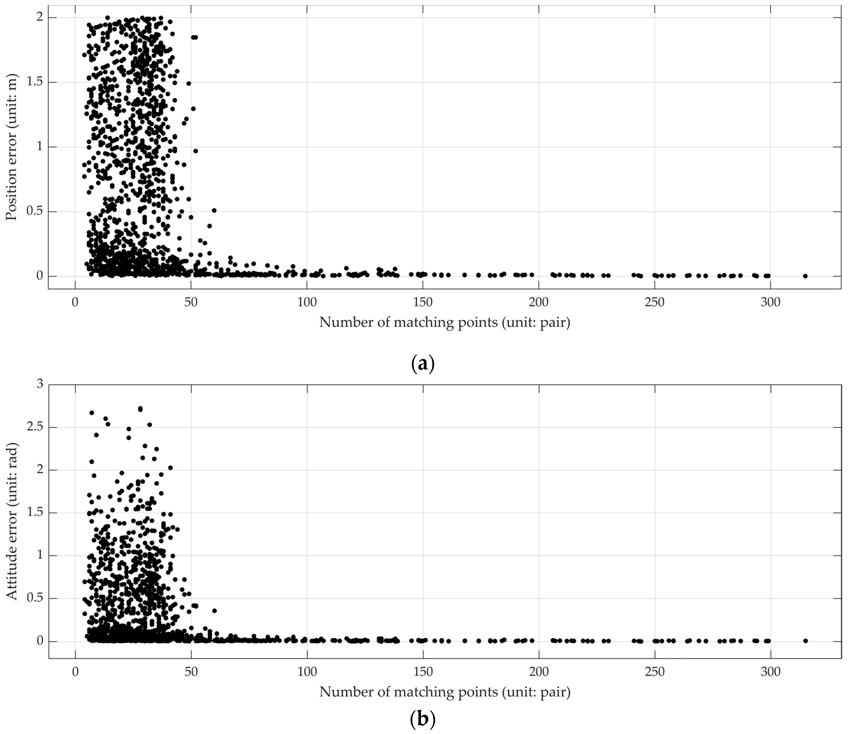
First, the relationship between pose error and number of matching points is a key criterion of the proposed process. The pose of each query image was calculated by means of the visual-positioning process mentioned in
Section 2.3. The number of matching points was recorded in this positioning process. The pose error was obtained by comparing the calculated pose with its ground truth. After testing all the query images, pose errors and corresponding number of matching points for each query image were collected and analyzed to determine their relationship (
Figure 2). It is found from
Figure 2a,b that both the position error and attitude error fluctuate greatly when the number of matching points is less than 50. However, when the number of matching points is more than 50, the pose errors are basically stable at a small value. In other words, our visual-positioning process can obtain precise and stable results when the number of matching points is more than 50. So we set 50 as the threshold
for the minimum number of matching points.
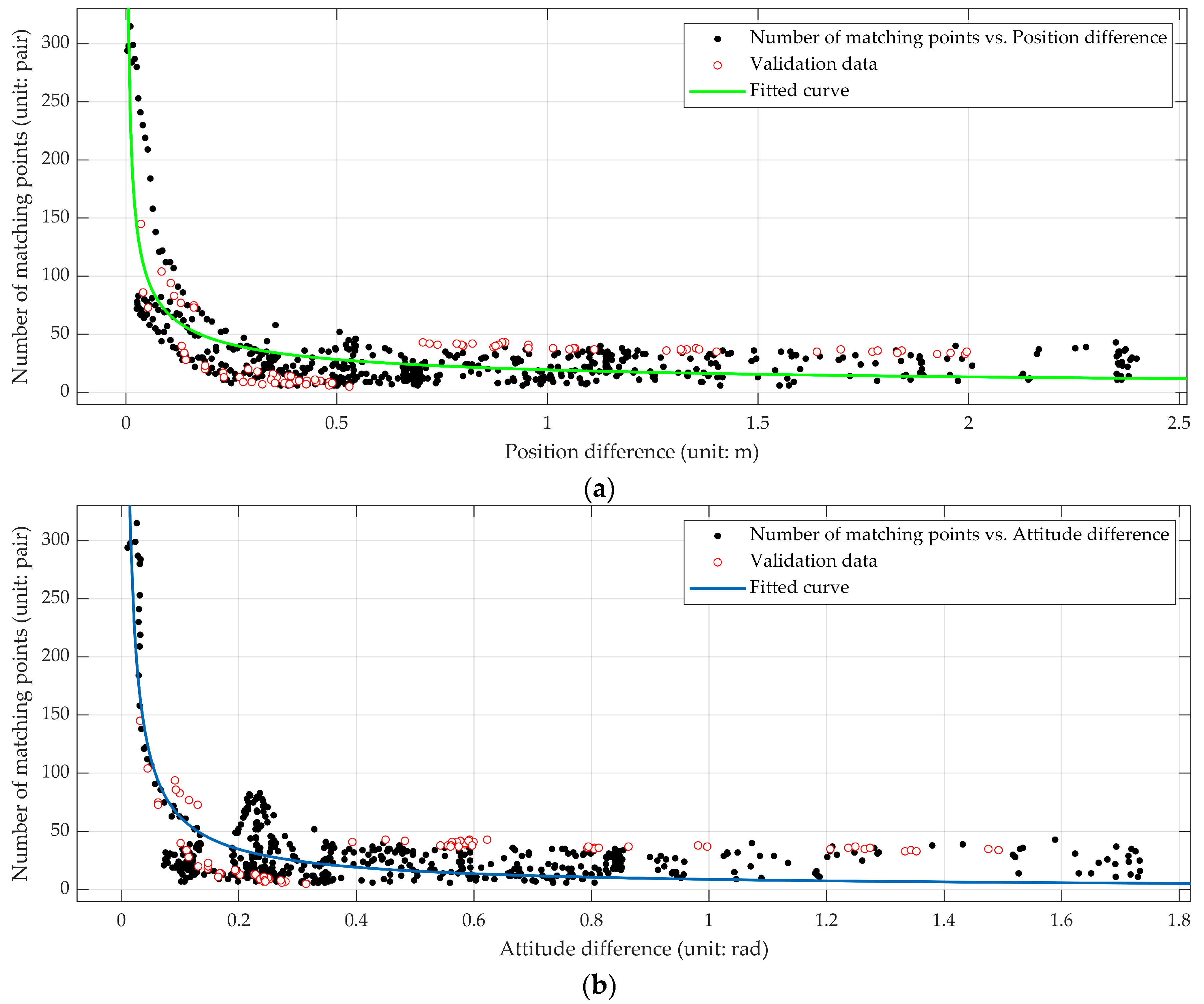
Second, the relationship between number of matching points and pose difference is also an important criterion in the RGB-D image database construction process. The pose difference was calculated by comparing the ground truth pose of each query image with corresponding database image. Then the pose differences of some images were combined with their number of matching points to fit their relationship. The green fitted curve in
Figure 3a shows the fitted relationship between the number of matching points and position difference. Its expression is described as follows:
Here
is position difference,
is the number of matching points. The blue fitted curve in
Figure 3b shows the fitted relationship between the number of matching points and attitude difference. Its expression is described as Equation (2):
Here
is attitude difference,
is the number of matching points. Then we used some other pose differences and number of matching points of more than seventy images to validate Equations (1) and (2). As shown in
Figure 3a,b, the validation data are distributed near the fitted curve. The root mean square errors (RMSE) of fit and validation are shown in
Table 1.
We can see that the RMSE of validation data is close to the RMSE of fitted curve, which indicates that the fitted curves described in Equations (1) and (2) are applicable to different image data in the same scene. The empirical models are not sensitive to the selection of the query image, the established relationships are reliable to apply in the same scene.
From the trends of the fitted curves in
Figure 3, the number of matched points decreases as both of the position difference and attitude difference increase. According to the threshold
for the number of matching points from
Figure 2, the threshold of position difference
(i.e., the
in Equation (1)), and the threshold of attitude difference
(i.e., the
in Equation (2)), were obtained by substituting
and
with
. The results are as follows:
Based on these three thresholds
,
and
, the RGB-D image database construction process was proposed for indoor visual positioning (
Figure 4).
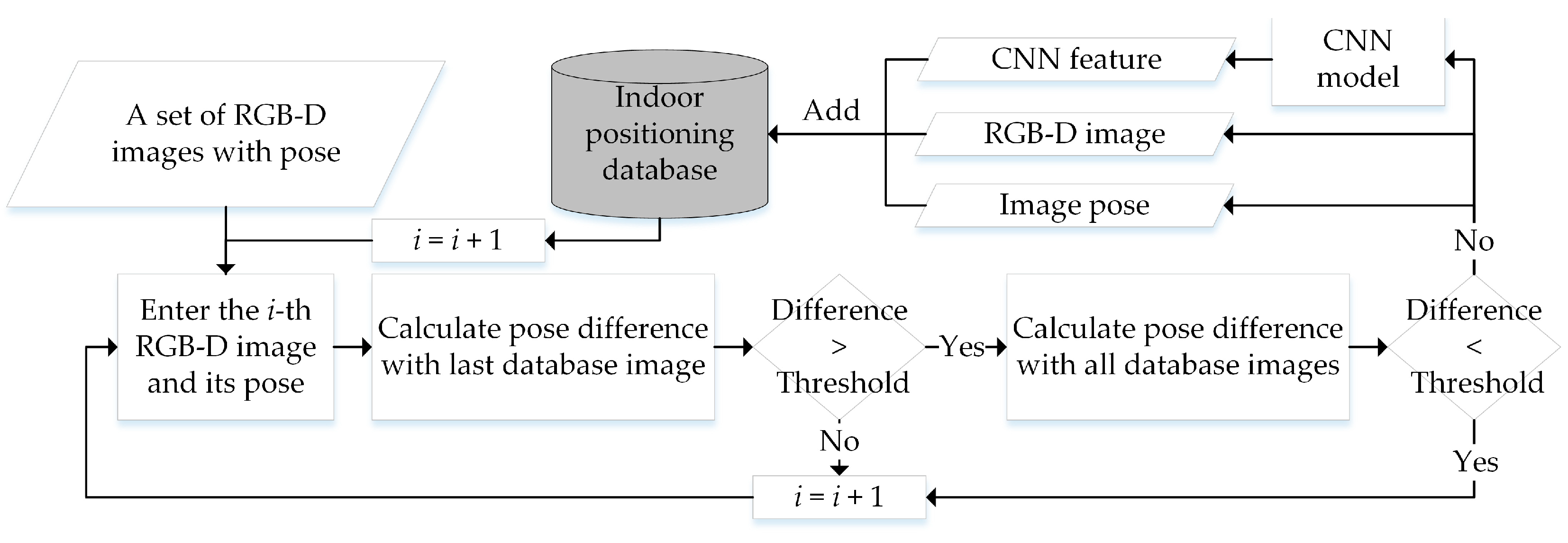
As shown in
Figure 4, first we need to input a set of RGB-D images with known poses in the scene where conducting indoor positioning. The RGB-D images can be captured using a Microsoft Kinect sensor and the ground truth trajectory of camera pose can be obtained from a high-accuracy motion-capture system with high-speed tracking cameras as in reference [
51]. In the database construction process, the first RGB-D image is considered as a database image and the other images will be input successively to determine whether they are required to join the database. From
Figure 4, the
i-th RGB-D image is compared with the last database image joining the database and then compared with all the existing database images to calculate the differences in position and attitude. If the differences meet the preset threshold condition (i.e.,
and
), the
i-th image will be determined as a new database image. It will be also input into the CNN model mentioned in
Section 2.2 to calculate its CNN feature vector for subsequent step of image retrieval. Finally, we add the three components of the eligible image into the indoor-positioning database, and then move on to the next RGB-D image until all images are judged.
The three components of the indoor positioning database are listed as follows. The first one is the RGB-D database images that meet the requirements. The second one is the corresponding pose information of database images. The here includes 3D position and quaternion form of attitude . The last one is the CNN feature vector set of database images.
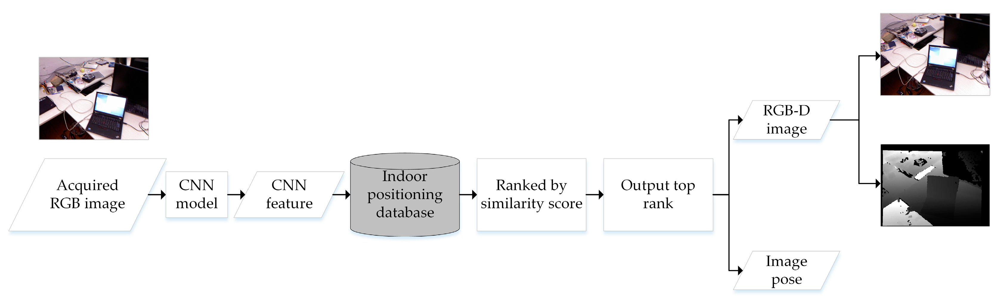
2.2. Image Retrieval Based on Convolutional Neural Network (CNN) Feature Vector
After building the indoor positioning database, it is important to know which RGB-D image in the database is the most similar to the input query RGB image acquiring by the mobile platform. The query RGB image and its most similar RGB-D image will be combined for conducting the subsequent visual positioning. In this sub-section, the CNN model and CNN feature vector-based image-retrieval algorithm were used in our indoor positioning method. We adopted the CNN architecture proposed in reference [
52], the main component of which is a generalized vector of locally aggregated descriptors (NetVLAD) layer and it is readily pluggable into standard CNN architecture. The best performing network they trained was adopted to extract image deep features, i.e., CNN feature vector, for image retrieval in this study.
Figure 5 shows the process of image retrieval based on CNN feature vector. With this process, the RGB-D database image, which is the most similar to the input query image, and its pose information were retrieved. First, in
Section 2.1, we have calculated and saved the database CNN feature vector set
in the indoor positioning database. When a query color image
with the same size as the database images is input, the same CNN model is used to calculate its CNN feature vector. This output CNN feature vector
of query image has the same length with the feature vector
of the database image. In this research, the size of CNN feature vector is
.Then the distance between
and each feature vector of
is calculated to represent their similarity, which is defined as follows:
The set of distances is . Finally, we output a retrieved RGB-D database image and its pose information , which has the minimum distance with the query color image.
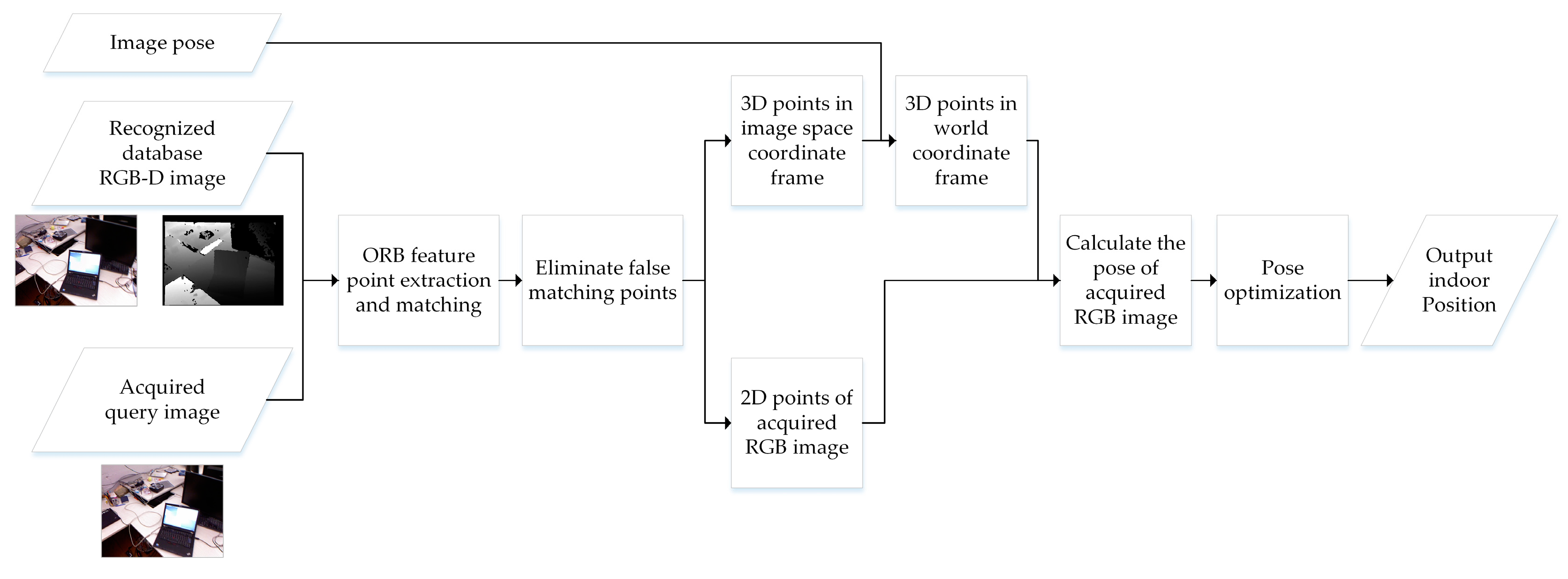
2.3. Position and Attitude Estimation
After retrieving the most similar RGB-D database image with an acquired query RGB image, the visual positioning was achieved by estimation of the position and attitude of the query image based on the retrieved database image and its pose information (
Figure 6).
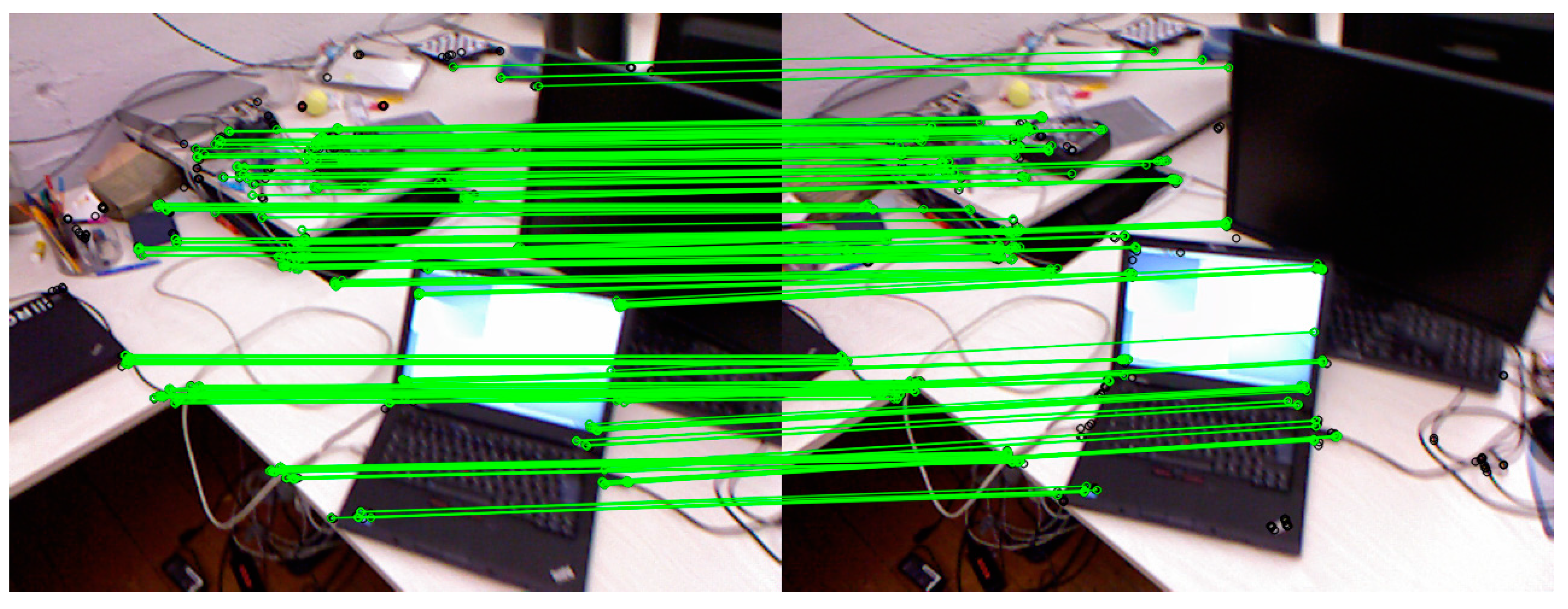
In
Figure 6, feature point extraction and matching between the acquired query image and the retrieved database image is the first step in the visual-positioning process. The ORB algorithm was adopted in our method to extract 2D feature points and calculate binary descriptors for feature matching. Then, the fundamental matrix constraint [
53] and random sample consensus (RANSAC) algorithm [
54] were used to eliminate some false matching points. After that, two sets of good matching points
and
in the pixel coordinate frame were obtained.
Figure 7 shows the result of good matching points between the acquired query image and the retrieved database image.
Second, 3D information in the world coordinate frame of the matching points was obtained by the retrieved RGB-D database image and its image pose. A feature point
belonging to
in the retrieved database image is a 2D point in the pixel coordinate frame. Its form in the image plane coordinate frame
is obtained by Equation (5):
Here
,
,
and
belong to the intrinsic parameters
of camera, which was calculated through camera calibration process. Through the depth image of the retrieved RGB-D database image, we obtained the depth value
of
. Therefore, the 3D point
in the image space coordinate frame is obtained by Equation (6):
Next, the input pose information
of the retrieved image is used to translate
into the world coordinate frame. The
here includes 3D position
and quaternion form of attitude
. Usually
is expressed as a transformation matrix
from image space coordinate frame to world coordinate frame by Equation (7):
where
and
are the rotation and translation parts of
respectively.
is defined as follows:
Then
is used to transform
into the world coordinate frame
:
So the relationship between a 3D point
in the world coordinate frame and its 2D point
in the pixel coordinate frame is expressed as follows:
Here, matrices
,
and
are the inverse of matrices
,
and
respectively. By using the relationship described in Equation (10), we calculated a set of 3D points
in the world coordinate frame corresponding to the set of 2D points
in the retrieved image. Because
and
are two sets of matching points,
is also corresponding to
.
Third, according to the 2D matching points and their 3D points in the query image, the efficient perspective-n-point (EPnP) method [
55] was adopted to estimate the initial pose
of the query image. The Levenberg–Marquardt algorithm implemented in g2o [
56] was then used to optimize the camera pose iteratively. This process can be described as follows:
Here
is the
i-th 2D point of
and
is the
i-th 3D point of
. The number
is the length of
. The poses got from the EPnP method were used as the initial values of
.
Through iteration, an optimized pose result of the query image was obtained. And we inverted to get , because is more intuitive, from which we can directly get the pose of the query image. Finally, was saved in the form of , where and are the position and attitude of the query image respectively.
With this process, the precise and real-time position and attitude of the acquired query color image were estimated. In the following experimental section, we performed abundant experiments to verify the accuracy of our indoor-positioning method in common indoor scenes.
3. Experimental Results
We have conducted a series of experiments to evaluate the effectiveness of the proposed indoor positioning method. The first sub-section describes the test data and computer configuration we used in the experiments. In the second sub-section, we evaluate qualitatively the proposed RGB-D image database construction strategy of our indoor positioning method. And the results are reported in the third sub-section. For a complete comparative analysis, the results of our indoor positioning method are also compared with an existing method in reference [
50].
3.1. Test Data and Computer Configuration
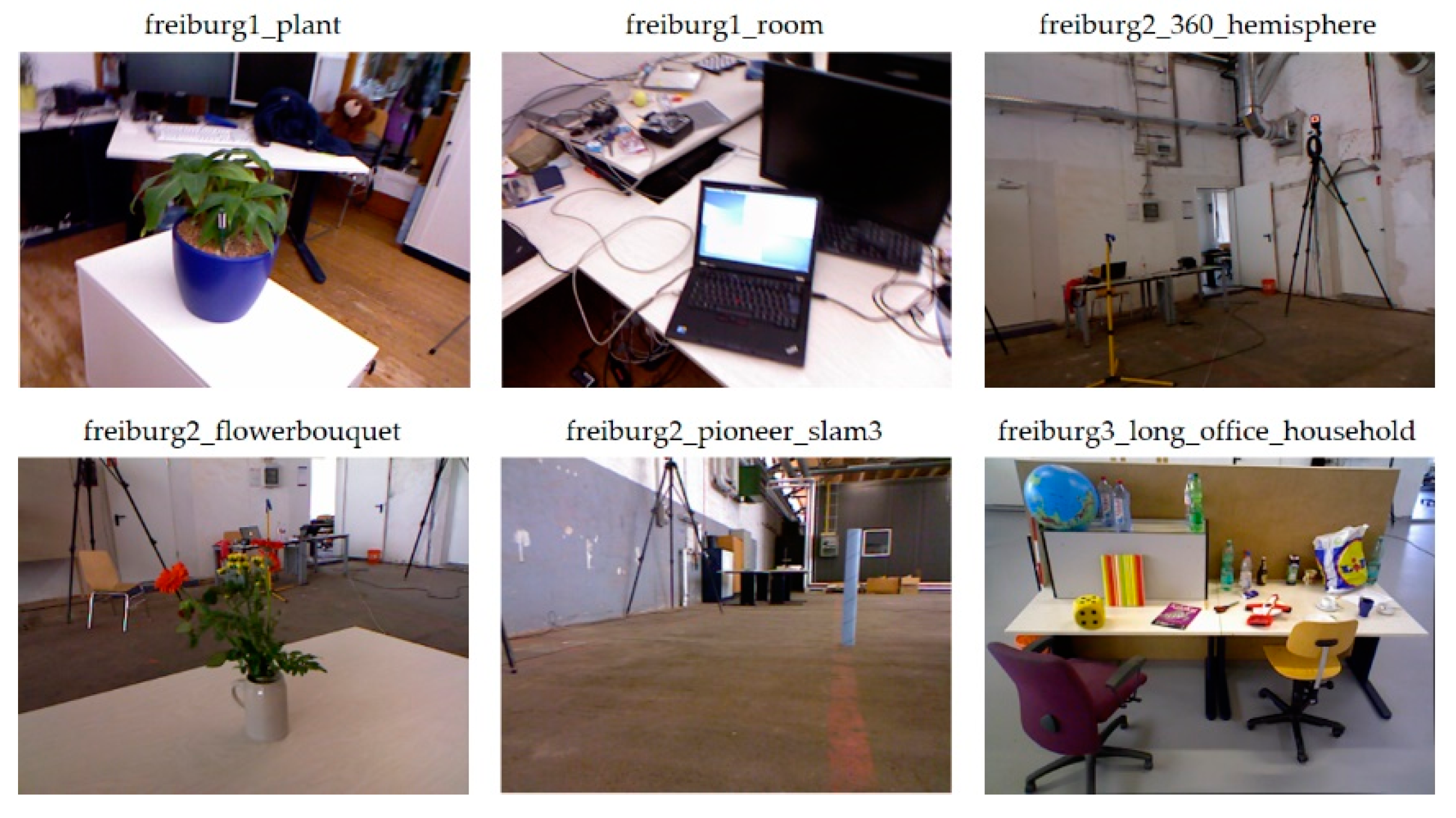
In order to better evaluate the proposed indoor positioning method, six sequences of the public dataset TUM RGB-D were adopted as the test data. Every sequence of the dataset contains RGB-D images, i.e., RGB and depth images, captured by a Microsoft Kinect sensor at a frame rate of 30 Hz. The size of the RGB-D images was .
Figure 8 shows the six sequences of TUM RGB-D dataset. These six sequences can well represent the common indoor scenes in daily life. And the intrinsic parameters of the Microsoft Kinect sensor were found in reference [
51].
Before the procedure of RGB-D image database construction, it was important to determine the availability of these sequences. If the associated depth image of a RGB image was missing, then the RGB image was discarded. After that, the remaining test images were used in the experiments of database construction and pose estimation. Then the database images corresponding to the query images with large pose errors were checked manually. If they were motion blur or poorly illuminated images, they were removed from the database. The number of test images in each of these six sequences is shown in
Table 2.
We employed a computer with an Intel Core i7-6820HQ CPU @ 2.7 GHz and 16 GB RAM to conduct all the experiments. The procedure of image retrieval based on CNN feature vector was accelerated by a NVIDIA Quadro M2000M GPU. The details of the experimental results are described below.
3.2. Results of RGB-D Database Construction
According to the RGB-D database construction process described in
Section 2.2, we got the constructed databases of six sequences shown in
Figure 9. The gray lines represent the ground truth of trajectories when recording RGB-D images. The red hexagonal points on the gray lines are the positions of indoor-positioning database images. As can be seen from
Figure 9, more database images are selected using the proposed database construction method at the corners where the position and attitude differences between neighboring recorded images change greatly. In these areas with smooth motion, the database images selected by our method are evenly distributed. After selecting the database images from the test images of six sequences, the remaining images were used as query images to conduct the subsequent visual-positioning experiments.
Considering the redundancy of the RGB-D test images and the efficiency of the visual positioning process, most methods are implemented by selecting representative database images manually, as in reference [
50]. The method of hand-pick is subjective and time-consuming. The quality of the database images depends largely on experience. When the number of captured images is large, the workload increases. In contrast, the database images selected by the proposed RGB-D image database construction process are not too redundant or sparse. The database image directly provides high accuracy depth information, this not only ensures high accuracy of positioning, but also improves the efficiency of image retrieval. Therefore, the proposed method can reduce the workload of selecting representative database images and meet the requirements of highly accurate and real-time indoor positioning.
The hand-picked database images of reference method [
50] are used for comparison. The numbers of selected database images and used query images in the reference method and the proposed method are shown in
Table 3. It can be seen from
Table 3 that the number of query images used in our method is about twice the number of query images used in the reference method. This is because the proposed method automatically selects the database images and then takes the remaining images as query images, eliminating the workload of manually selecting images.
After building the RGB-D indoor-positioning database, we input query images of each sequence in turn. Through the process of image retrieval based on the CNN feature vector, we selected a database RGB-D image with pose information that is most similar to the input query image. Then we performed the visual-positioning process to estimate the position and attitude of each input query image.
3.3. Quantitative Analysis of Positioning Accuracy
In this part, the performance of pose estimation in the proposed indoor-positioning method was evaluated by comparing it with the reference method mentioned in the previous section. The estimated pose results of each sequence was saved in a file. The mean pose error and median pose error of these two methods were obtained by comparing the estimated poses with the ground truth trajectory. In addition, both position error and attitude error were calculated as an evaluation of six DoFs.
The pose estimation results of each sequence using the reference method and proposed method are shown in
Table 4. As can be seen from the results of the proposed method in
Table 4, the mean values and median values of position errors are both at the half-meter level. As for attitude errors, the mean errors are within 5 degrees and the median errors are within 1 degree. These results demonstrate that the database we built in
Section 3.2 meets the requirements of high-accuracy visual positioning well. By comparing the results of the reference method and the proposed method, we can see that most of the mean and median pose errors of our method are smaller than those of the reference method. This also indicates that the database constructed by our method can achieve or surpass the accuracy of the hand-picked database to some extent.
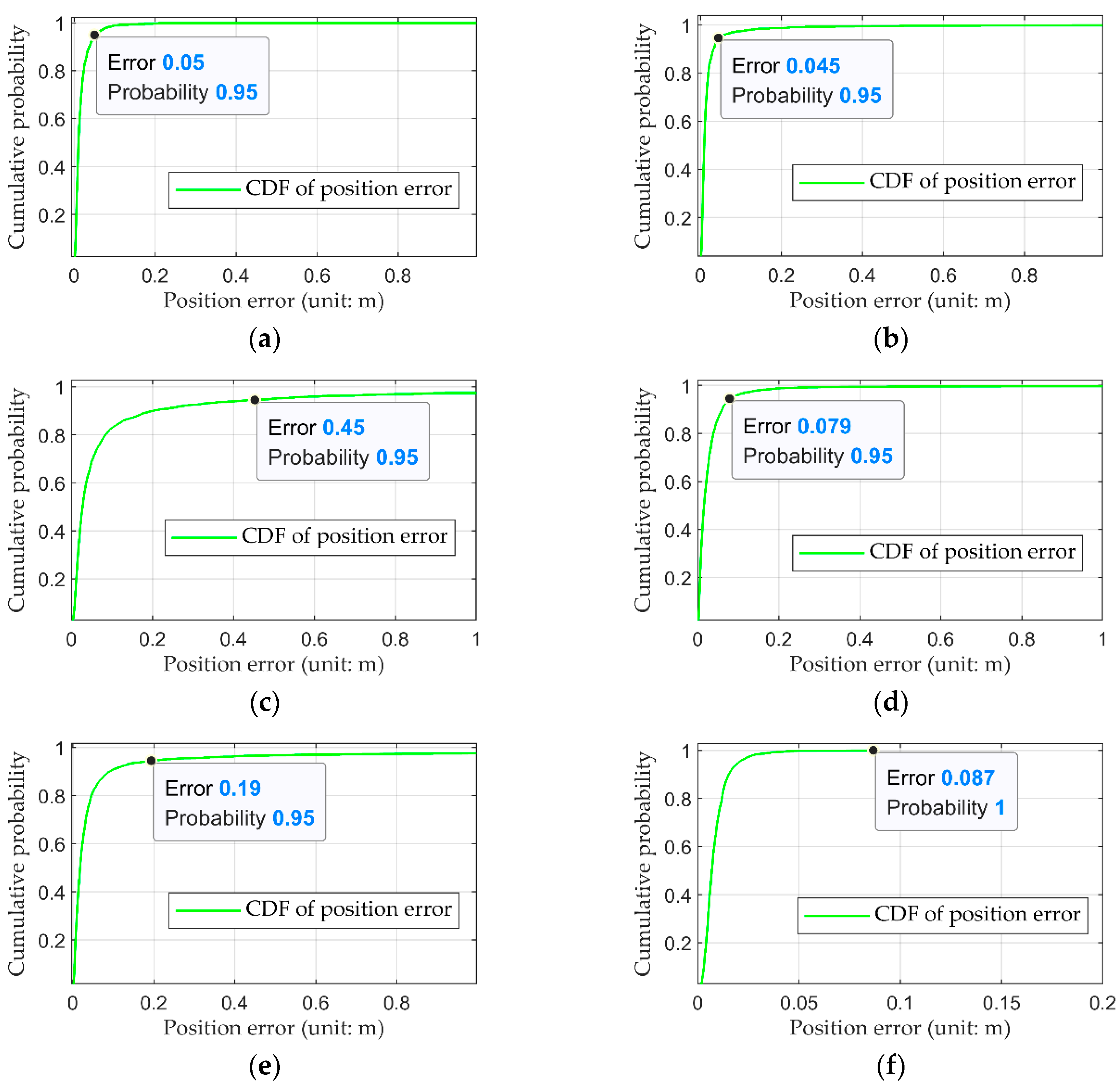
In order to demonstrate the pose estimation results of all the query images intuitively, cumulative distribution function (CDF) was adopted to analyze the positioning accuracy of the proposed method.
Figure 10 shows the CDF of position error. From these CDF curves we can see that nearly 95% of the query images have a position error within 0.5 m. Furthermore, the position errors of all query images in sequence freiburg3_long_office_household are within 0.1 m, as shown in
Figure 10f. These results show that the proposed method is able to localize the position of a query image well and achieve a high accuracy of better than 1 m in most cases.
In addition to CDF of position error, CDF of attitude error was also calculated as an evaluation of six DoFs.
Figure 11 shows the CDF of attitude error. The blue line of each sub-figure represents the CDF curve. Similarly, we can see that the attitude errors of all query images in sequence freiburg3_long_office_household are within 3 degrees, as shown in
Figure 11f. For the rest of the sequences, almost 95% of the query images have an attitude error within 5 degrees. These results show that the proposed method is able to calculate the attitude of a query image well with an accuracy of better than 5 degrees in most cases.
The cumulative pose errors of the reference method and the proposed method were compared, as shown in
Table 5. It was found that most of the results using our method outperformed those using the reference method. As can be seen from the cumulative accuracy of the reference method, 90% of the query images in each sequence are localized within 1 m and 5 degrees. The 90% accuracy of position error of our method is within 0.5 m and the attitude error is within 3 degrees, both of which are nearly half the pose error of the reference method. Specifically, all the cumulative position errors of the proposed method are better than those of the reference method. The cumulative attitude errors of the proposed method are better or comparable with those of the reference method. These good performances of the proposed indoor visual-positioning method also indicate the validity of the proposed database construction strategy.
All the experiments were conducted by a laptop with an Intel Core i7-6820HQ CPU @ 2.7 GHz and 16 GB RAM. In the experiment, it takes about 0.4 s on average to implement the RGB-D database image-retrieval process in selecting the most similar database image with the input query image. The pose estimation process of one query image takes about 0.2 s on average. Considering that the RGB-D indoor positioning database is built offline, the time it costs is not taken into account. Therefore, our indoor-positioning program will take about 0.6 s to complete the two processes of image retrieval and pose estimation. Specifically, if we use a mobile platform to capture query image at a resolution of and upload it into the laptop using 4G network, the process takes about 0.3 s. As for returning the location result from the laptop to the mobile platform, it takes about 0.1 s. Therefore, the whole procedure, which starts with capturing a query image by the mobile platform and finally obtains the position result from the laptop, takes about 1 s. In other words, the indoor-positioning frequency of the proposed method is about 1 Hz. This also shows that the proposed method has the ability of real-time indoor positioning while satisfying the need for high accuracy.
4. Conclusions
In this study, a novel indoor-positioning method with automated RGB-D image database construction was presented. The proposed method has two main innovations. First, the indoor-positioning database constructed by our method can reduce the workload of manually selecting database images and is more objective. The database is automatically constructed according to the preset rules, which reduces the redundancy of the database and improves the efficiency of the image-retrieval process. Second, by combining automatic database construction module, the CNN-based image retrieval module, and strict geometric relations based pose estimation module, we obtain a highly accurate indoor-positioning system.
In the experiment, the proposed indoor positioning method was evaluated with six typical indoor sequences of TUM RGB-D dataset. We presented the quantitative evaluation results of our method compared with a state-of-the-art indoor visual-positioning method. All the experimental results show that the proposed method obtains high-accuracy position and attitude results in common indoor scenes. The accuracy of the proposed method attained is generally higher than that of the reference method.
In the next version of our indoor-positioning method, we plan to combine the semantic information of the sequence to reduce the search space of visual positioning in large indoor scenes.


