Evaluation of MWHS-2 Using a Co-located Ground-Based Radar Network for Improved Model Assimilation

Abstract

Accurate precipitation detection is one of the most important factors in satellite data assimilation, due to the large uncertainties associated with precipitation properties in radiative transfer models and numerical weather prediction (NWP) models. In this paper, a method to achieve remote sensing of precipitation and classify its intensity over land using a co-located ground-based radar network is described. This method is intended to characterize the O−B biases for the microwave humidity sounder -2 (MWHS-2) under four categories of precipitation: precipitation-free (0–5 dBZ), light precipitation (5–20 dBZ), moderate precipitation (20–35 dBZ), and intense precipitation (>35 dBZ). Additionally, O represents the observed brightness temperature (TB) of the satellite and B is the simulated TB from the model background field using the radiative transfer model. Thresholds for the brightness temperature differences between channels, as well as the order relation between the differences, exhibited a good estimation of precipitation. It is demonstrated that differences between observations and simulations were predominantly due to the cases in which radar reflectivity was above 15 dBZ. For most channels, the biases and standard deviations of O−B increased with precipitation intensity. Specifically, it is noted that for channel 11 (183.31 ± 1 GHz), the standard deviations of O−B under moderate and intense precipitation were even smaller than those under light precipitation and precipitation-free conditions. Likewise, abnormal results can also be seen for channel 4 (118.75 ± 0.3 GHz).

1. Introduction

Polar-orbiting satellite observations in the visible, infrared, and microwave spectra provide a great deal of information on clouds and precipitation, as well as atmospheric water vapor and temperature [1,2,3]. In operational numerical weather prediction (NWP) models, microwave and infrared radiances from polar-orbiting satellite instruments are routinely assimilated to improve the accuracy of short-range and medium-range forecasts [4,5,6]. It was found that assimilating radiances of microwave humidity and temperature sounders such as the advanced technology microwave sounder (ATMS) could improve the prediction of humidity, temperature, and wind fields in the middle and high troposphere [7,8].

Since satellite data assimilation is based on the underlying assumption that both observation (O) and simulation (B) are unbiased and that Gaussian error statistics and a linear relationship exist between them [9,10]. Satellite-observed radiances are directly assimilated into the NWP model using a computationally efficient, optimum procedure which minimizes the difference between the radiances observed (i.e., O) and those radiances computed (i.e., B) based on the NWP output of the atmospheric state [11]. Any bias related to the instrument and model simulations needs to be quantified, then removed, in satellite data assimilation. Therefore, it is necessary to estimate the biases of the instrument and the model before assimilating the satellite data.

There are a variety of reasons accounting for biases of O and B. On the one hand, observation biases (${\mu }^o$) can arise from calibration errors in a satellite sensor, instrument “drift” as a sensor ages, and the presence of cloud and precipitation. On the other hand, simulation biases (${\mu }^b$) can also be introduced by deficiencies in the radiative transfer models in the specification of surface emissivity, simplifications in the radiative transfer model equations, misspecification or absence of atmospheric constituents such as aerosols and hydrometeors, and the biases in background filed from the NWP model. In brevity, the observation biases and simulation biases can be lumped together and expressed as $\left(\mathrm{O}-{\mu }^o\right)-\left(\mathrm{B}-{\mu }^b\right)=\mathrm{O}-\mathrm{B}-\left({\mu }^o+{\mu }^b\right)$. Thus, O−B statistics can be used to estimate the sum of observation and simulation biases ${\mu }^o+{\mu }^b$ [12].

Currently, satellite assimilation is mostly conducted under clear skies [13]. Direct assimilation of cloudy and precipitating radiances may result in larger uncertainties in both NWP and radiative transfer models due to cloud and precipitation processes which may interact nonlinearly with the complex thermodynamic environment. Most of the existing cloud and precipitation screening-out methods in quality control processes are widely carried out over oceans to derive the ice water path (IWP) [14], liquid water path (LWP) [15], and scattering index (SI) [16] from window channels. However, the percentage of observations made with completely clear skies is often less than 20%, and exclusion of cloudy and precipitating measurements has the undesirable consequence of removing observations that could have been used to improve the model initialization in cloudy and precipitating areas of the model domain [17]. Thus, it is critical to develop radiative transfer models with well-understood error characteristics not only under clear-sky conditions, but also under cloudy and precipitating conditions, and to further quantify and reduce the errors to effectively incorporate microwave radiances under cloudy and precipitating conditions in operational data assimilation [18,19]. Thus, both accurate cloud and precipitation detection methods and proper characterization of O−B biases are essential for the application of assimilating cloud- and precipitation- affected radiances.

A cloud detection method that co-locates measurements from the advanced microwave sounding unit-A (AMSU-A) and ATMS with high spatial resolution cloud products from a moderate resolution imaging spectroradiometer (MODIS) and visible infrared imager radiometer suit (VIIRS) was presented by Han et al. [20]. This method improves the accuracy of tropical cyclone forecasts and radiance assimilation by better eliminating cloud-contaminated microwave sounder field-of-views. Chen et al. [21] used CloudSat data under non-precipitation cloudy conditions to validate the accuracy of the community radiative transfer model (CRTM), and they found that the O−B biases and standard deviation errors are low for advanced very high resolution radiometer (AVHRR) channels 4 and 5, but became lager under cirrus and mixed-phase cloudy conditions. On the other hand, the O−B biases for the microwave humidity sounder (MHS) on board National Oceanic and Atmospheric Administration -18 (NOAA-18) from 89 GHz to 190 GHz under cloudy conditions are only marginally different from those under clear skies [21], possibly due to the fact that microwave radiation can penetrate through clouds, other than thick clouds and precipitation [20,22,23,24]. It was implied that the large O−B biases should be attributed to precipitation rather than cloud.

Though forward radiative transfer models (e.g., CRTM) for clear and cloudy scenes have become more accurate recently, deficiencies remain, especially for precipitating conditions. In this study, the characteristics of O−B biases for MWHS-2 under precipitating conditions were evaluated. Then special attention was given to the detection methods of precipitation. As mentioned above, most existing precipitation detection methods are widely carried out over the ocean. However, precipitation detection over land becomes much more challenging due to the much larger emission from land surface than from precipitation. With the significant development of the China new-generation weather radar (CINRAD), it is expected that radar reflectivity has the potential to improve the detection of precipitation particles and classification of precipitation intensities without the influence of surface emissivity over land. This study focused on O−B biases under different intensities of precipitation over land, aided by ground-based radar measurements.

This paper is organized as follows. Section 2 briefly describes the data and methodology. No precipitation (0–5 dBZ), light precipitation (5–20 dBZ), moderate precipitation (20–35 dBZ), and intense precipitation (>35 dBZ) are classified using eight weather radars. Section 3.1 shows the sensitivity of brightness temperatures (TB) and brightness temperature differences between channels (∆TB) to radar reflectivity. Section 3.2.1 presents a simple quality control procedure for exclusion of those data for which the comparison of O and B is extremely large. Section 3.2.2 assesses the characteristics of O−B biases for MWHS-2 under different classes of precipitation conditions. Section 4 discusses the interpretation of the results. Section 5 summarizes the study and draws conclusions.

2. Data and Methodology

2.1. MWHS-2 Channel Characteristics

The Feng Yun series 3 (FY-3) satellite developed by the China Meteorological Administration (CMA) is a new generation of sun-synchronous polar-orbiting satellite series consisting of seven satellites. FY-3A and FY-3B were experimental satellites and were launched on May 27, 2008 and December 5, 2010, respectively. FY-3C and FY-3D were operational satellites and were launched on September 23, 2013 and November 15, 2017, respectively. Both FY-3A and FY-3C were configured in morning orbits with local equator crossing times (LECT) around 10 a.m., and FY-3B and FY-3D were in an afternoon orbit with the LECT around 2 p.m. The MWHS-2 on board FY-3C/D is an advanced microwave humidity sounder with the first operational space-borne use of 118.75 GHz. The MWHS-2 on board FY-3C is of special interest in this study since it works stably to provide accurate atmospheric temperature and humidity data.

MWHS-2 is a 15-channel cross-track scanning microwave radiometer. Channel number, central frequencies, beam widths, and the peaking weighting functions (WFs) for the 15 channels of MWHS-2 are provided in

Table 1. Instrument characteristics of the microwave humidity sounder -2 (MWHS-2).

Channel	Center Frequency (GHz)	Beam Width (deg)	Peak Weighting Function (hPa)
1	89.0	2.0	surface
2	118.75 $\pm$ 0.08	2.0	20
3	118.75 $\pm$ 0.2	2.0	60
4	118.75 $\pm$ 0.3	2.0	100
5	118.75 $\pm$ 0.8	2.0	250
6	118.75 $\pm$ 1.1	2.0	300
7	118.75 $\pm$ 2.5	2.0	700
8	118.75 $\pm$ 3.0	2.0	surface
9	118.75 $\pm$ 5.0	2.0	surface
10	150.0	1.1	surface
11	183.31 $\pm$ 1	1.1	450
12	183.31 $\pm$ 1.8	1.1	500
13	183.31 $\pm$ 3	1.1	600
14	183.31 $\pm$ 4.5	1.1	700
15	183.31 $\pm$ 7	1.1	800

. MWHS-2 channels 1 and 10 are two window channels and are affected by emissions from the Earth’s surface and scattering from ice phase clouds. The five humidity-sounding channels near 183.31 GHz are primarily sensitive to humidity at different heights from 2 to 10 km in the troposphere. MWHS-2 channel 15 has the highest central frequency among the five humidity-sounding channels and is most sensitive to scattering from thin clouds. The other eight MWHS-2 channels are located at the oxygen absorption band near 118.75 GHz and are sensitive to temperature in the stratosphere (channels 2–4) and the troposphere (channels 5–9). Channel 7, which has a lower peaking WF, is also sensitive to humidity due to the water vapor continuum [25,26]. Channels 8 and 9 whose WFs peak near the surface were found to be highly surface sensitive and therefore can be essentially window channels. The altitude of FY-3C orbits is around 836 km. It has an inclination of 98.75°, an orbital period of 101.49 min, and 14.1735 orbits/day. The quasi-repeat time is about five days. The antenna of MWHS-2 scans within the angles of ±53.35°, leading to a swath width of ~2600 km. There is a total of 98 field-of-views (FOVs) along each scan line. The nominal spatial resolutions of MWHS-2 are 15 km at nadir for channels 10–15 and 33 km for channels 1–9.

2.2. The Weather Radar Network

The new-generation weather radar (CINRAD) network in China includes more than 200 Doppler weather radars and has played an important role in disaster weather monitoring since 1998. CINRAD consists of two bands, C-band in inland regions and S-band in coastal regions. In order to classify O−B biases with different precipitation intensities, eight S-band weather radars were selected: GRFY (Ground radar in Fuyang, Anhui Province); GRHF (Ground radar in Hefei, Anhui Province); GRXZ (Ground radar in Xuzhou, Jiangsu Province); GRNJ (Ground radar in Nanjing, Jiangsu Province); GRLYG (Ground radar in Lianyungang, Jiangsu Province); GRYC (Ground radar in Yancheng, Jiangsu Province); GRNT (Ground radar in Nantong, Jiangsu Province); and GRHZ (Ground radar in Hangzhou, Zhejiang Province) in East China (Figure 1). These radars were all China new-generation weather radar S-band A-type (CINRAD-SA) with a wavelength of ~10 cm and effective precipitation detection distance of ~230 km. All ground radars operated volume scans of nine elevation angles from 0.5$°$ to 19.5$°$. The radar reflectivity factor mosaic from these eight weather radars can be used to categorize different intensities of precipitation.

2.3. The Community Radiative Transfer Model (CRTM)

The community radiative transfer model (CRTM) [11,27] developed by the US Joint Center for Satellite Data Assimilation (JCSDA) was used in this work to simulate brightness temperatures of MWHS-2. This model has been widely used for microwave and infrared satellite data assimilation and remote sensing applications, as well as aerosol assimilation [28,29]. It includes modules that compute the satellite-measured radiation from gaseous absorption, and scattering of radiation by aerosols and clouds, as well as emissions and reflection of radiation by the Earth’s surface. Moreover, the corresponding tangent linear and adjoint operators were already included in the CRTM package released.

In this study, analysis data from the European Center for Medium-Range Weather Forecasting (ECMWF) [20] were used as background fields of CRTM for clear-sky scenario simulations. The ECMWF dataset has a horizontal resolution of 0.5° × 0.5° and 37 levels in the vertical direction with the top-level pressure approximately at 1 hPa. Input background variables include the 10 m wind component, the surface skin temperature, the surface pressure, the air pressure at the Earth’s surface and in the atmosphere, the water vapor mixing ratio, the atmospheric temperature, and the ozone concentration. Additionally, the instrument parameters of MWHS-2, such as the scan angle and zenith angle, were also inputted to CRTM.

2.4. Combined Satellite and Radar Dataset

In this study, the radar reflectivity of the eight combined weather radars in East China, as described above, was co-located with MWHS-2 field-of-view (FOV), so that each FOV had a corresponding radar reflectivity value to classify precipitation intensity. As shown in

Table 2. Description of different precipitation intensities used in this study. The number of MWHS-2/Ground-based radar coincident observations for each category (N_obs) is also shown.

Class	Radar Reflectivity	Type of Precipitation	Nobs
1	0–5 dBZ	No precipitation	6536
2	5–20 dBZ	Light precipitation	2491
3	20–35 dBZ	Moderate precipitation	1758
4	>35 dBZ	Intense precipitation	468

, each observation was assigned to one of four classes: precipitation-free (0–5 dBZ), light precipitation (5–20 dBZ), moderate precipitation (20–35 dBZ), and intense precipitation (>35 dBZ). The dataset was sampled from 13 precipitating cases during the time period from July to September in 2016, over land. In order to provide a greater number of observations in the intense precipitation category (>35 dBZ), the cases with heavy rainfall and radar reflectivity above 35 dBZ, according to 24-h rainfall and radar composite reflectivity dataset, were selected accordingly.

The key technologies for the combined application of radar and satellites are radar data quality control, generation of mosaic reflectivity for multiple radars, and spatial matching. In order to eliminate noise, biological echoes, clutter/anomalous propagation echoes and reflectivity biases, the radar dataset was subjected to a median filter, a fuzzy logic clutter filter (https://www.weather.gov/code88d/) and reflectivity bias correction [30,31]. The Severe Weather Nowcast System (SWAN) [32] developed by CMA was used to generate mosaic reflectivity for eight radars. A standard latitude and longitude grid system (0.01° × 0.01°) was defined according to the study area. The radar dataset in polar coordinates was mapped to the standard grid system by SWAN, and the inverse distance weighting interpolation method was used to generate mosaic reflectivity. Finally, the mosaic reflectivity was mapped to the filed-of-view of satellite by using the bilinear interpolation method to obtain the radar-satellite match-up dataset.

3. Results

3.1. Sensitivity of Brightness Temperature to Radar Reflectivity

MWHS-2 features eight new temperature-sounding channels around the 118.75 GHz oxygen absorption line, along with five traditional humidity-sounding channels located near the 183.31 GHz water vapor absorption line [26]. It was pointed out that the brightness temperature at 118.75 GHz was much lower than that at 50–57 GHz, due to its strong frequency dependence on ice particle scattering in convective areas from the National Polar-Orbiting Operational Environmental Satellite System (NPOESS) aircraft sounder testbed-microwave (NAST-M) [33]. Therefore, the combination of 118.75 GHz and 183.31 GHz on MWHS-2 can allow profiling both temperature and humidity from a single instrument, and reveals more detailed features about hydrometeors related to cloud and precipitation, especially for ice particles.

Figure 2 and Figure 3 show the spatial distribution of ground-based radar reflectivity and satellite-observed brightness temperature for 15 channels of MWHS-2 for the case on 4 July 2016. It can be seen that the spatial distribution of radar measurements and brightness temperature of MWHS-2 were consistently correlated with respect to water vapor channels, window channels, and low-level temperature-sounding channels (channels 7–9). The averaged brightness temperature at window channels 1 and 10 was much higher than that of water vapor channels, due to the intense surface emissions in summer.

A very strong temperature depression is noticeable around the 33°N with brightness temperatures 40K lower than in the surrounding regions, highlighting a heavy hydrometer loading in this convective region, as shown in Figure 2a. In addition, channel 10 (150 GHz) shows even stronger sensitivity to precipitation-sized hydrometeors than channel 1 (89 GHz), especially when the radar reflectivity factor is above 25 dBZ. A significant temperature depression was also found for water vapor channels and channels 7–9. Channels from 11–15 and 7–9 responded to cloud and precipitation differently since the higher frequency channels probe deeper in the atmosphere, hence having greater depression in brightness temperature resulting from the scattering effect of hydrometeors. Additionally, this displays that brightness temperatures from low-level channels in the south of the study area are slightly larger than those in the north because higher temperatures exist near the equator in the summer, particularly for channels 7–10.

Figure 4a,b presents variations of brightness temperatures measured by MWHS-2 humidity-sounding and temperature-sounding channels versus radar reflectivity. Figure 4a shows that brightness temperatures for channels 11–15 in precipitating regions overall firstly increased and decreased subsequently, since emissions, scattering of clouds and precipitation could increase or decrease the brightness temperature.

As indicated in shaded region II in Figure 4a, brightness temperatures of channels 11–15 increase within 5–10 dBZ, illustrating that cloud emission dominates when rain rate is low and raindrop size is small. Then, brightness temperatures decrease with radar reflectivity as a result of the scattering effect by precipitation-sized hydrometeors as shown in region III and, more sharply, in region IV, due to the existence of larger hydrometeors.

The brightness temperature depression caused by the scattering effect of hydrometeors was different from channel to channel. Obviously, brightness temperature from channel 15 (TB₁₅) registered a stronger depression than the other four water vapor channels, presumably because the sensitivity of scattering to hydrometeors increased with frequency. Note that the brightness temperatures from channel 11 (183.31 $\pm$ 1 GHz) were even warmer than that from channel 15 (183.31 $\pm$ 7 GHz) above 35 dBZ. This is because channel 15 can see deeper into the cloud, and hence is subjected to greater scattering from the low layers of the cloud and precipitation. The differences in brightness temperature between channels 11–14 decreased with radar reflectivity, and the brightness temperatures for these channels tended to be ~230 K when the radar reflectivity reached 40 dBZ.

For MWHS-2 channels 2–6, whose weighting functions peaked mostly above 300 hPa, cloud and precipitation had negligible effects on brightness temperatures. Regarding channels 7–9, brightness temperatures in region II remained nearly constant and further decreased linearly with radar reflectivity in regions III and IV (Figure 4b). Note that TBs of channels 9 and 8 fell below that of channel 7 when radar reflectivity was above ~27 dBZ (the red line indicated in Figure 4b), mainly caused by different responses to hydrometeor size and content for these three channels.

From Figure 4, it can be seen that not only brightness temperatures (TB) but also the differences between these channels (∆TB) exhibited a good estimation of precipitation. Figure 5a,b shows the brightness temperature differences (∆TB) versus radar reflectivity for three humidity channels and temperature-sounding channels, respectively. It shows that the differences among brightness temperatures decreased with radar reflectivity in general. Regarding the humidity-sounding channels, brightness temperature differences between channels 15 and 13 (∆TB_15-13), channels 15 and 11 (∆TB_15-11), and channels 13 and 11 (∆TB_13-11) shifted from a positive to a negative value at points A1, A2, and A3, respectively (Figure 5a). It is also noticeable that the order of the ∆TB_15-13, ∆TB_15-11, and ∆TB_13-11 reversed at points B1 and B2. In terms of the temperature-sounding channels (Figure 5b), brightness temperature differences between channels 9 and 7 (∆TB_9-7), channels 9 and 8 (∆TB_9-8), as well as channels 8 and 7 (∆TB_8-7) declined linearly below 40 dBZ and approached 0 K at point C. When radar reflectivity was below ~27 dBZ, it was found that ∆TB_9-7 > ∆TB_9-8 > ∆TB_8-7 > 0 K existed because channels were further away from the center at 118.75 GHz and could see deeper into the troposphere where they detect higher temperatures in clear-sky and light precipitation. It is worth noting that the low-level sounding channels were subjected to greater scattering from cloud and precipitation and significant brightness temperature depression under moderate and intense precipitation conditions. Therefore, the relationship was reversed, ∆TB_9-7 < ∆TB_9-8 < ∆TB_8-7 < 0 K, where the radar reflectivity was above ~27 dBZ. This feature makes it evident that the order relation of the differences between brightness temperatures can provide a useful insight into precipitation intensity.

Figure 6 shows the scatter plots of ∆TB as a function of TB for channel 11 and channel 7, and the color of plots represents ground-based radar reflectivity. When radar reflectivity was above 15 dBZ, there was a tail of cases with decreasing TB and ∆TB. This is because brightness temperatures of low-level channels displayed a stronger depression in the presence of larger hydrometeors.

3.2. Evaluations of MWHS-2

3.2.1. Quality Control

It can be concluded from Section 3 that both observed TB and ∆TB had a strong dependence upon water vapor and hydrometeors, as shown by the radar reflectivity. To further study the characteristics of differences between O and B, a comparison of observations and simulations for TB and ∆TB was conducted as described below.

Figure 7 shows the joint probability density function (PDF) for TB and ∆TB, with the left column for observed values and the right column for simulated values. From Figure 7a,b, it can be seen that the maximum PDF is near the brightness temperature from channel 11 (TB₁₁) at ~240 K and ∆TB_13-11 at ~15 K. Figure 7c,d shows that the maximum of the PDF is near brightness temperature from channel 13 (TB₁₃) at ~255 K and ∆TB_13-11 at ~15 K. TB₁₁ at its maximum PDF is colder than TB₁₃, resulting from the fact that temperature decreased with height in the troposphere, and channel 11 was sensitive to a higher region than channel 13.

A considerable divergence exists between the observed and simulated brightness temperatures, with a long tail of decreasing ∆TB_13-11 and brightness temperatures. A similar distribution can also be seen for temperature-sounding channels 7 and 9 (Figure 7e–h). Figure 6 reveals that the tail cases with decreasing ∆TB_13-11 and brightness temperature mostly consist of radar reflectivity above 15 dBZ. Therefore, the scattering effect of hydrometeors above 15 dBZ, seen in the tail cases, resulted in the discrepancy between observations and simulations for both humidity- and temperature- sounding channels. The relationship between radar reflectivity and O−B is discussed in detail in Section 3.2.2.

Figure 8 presents scatter plots of MWHS-2 observations and CRTM simulations with ECMWF input profiles for channels 13 and 6. Before removing values above 15 dBZ, relatively significant differences were found between observations and simulations. However, the observations and simulations correlate quite well and linearly under the categories of 0–15 dBZ, and the linear correlation coefficients are greater than 0.8 and 0.9 for channels 13 and 6, respectively.

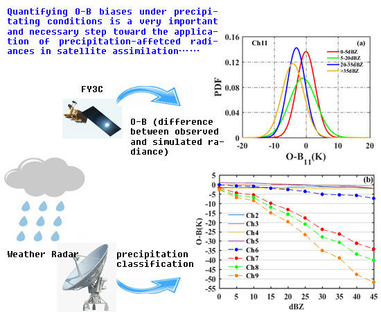
3.2.2. O−B Biases Characterization of MWHS-2 under Different Intensities of Precipitation

Figure 9 and Figure 10 display the spatial distributions of observed radar reflectivity and O−B for MWHS-2 channels. It can be seen that the spatial distribution of radar reflectivity above 15 dBZ and negative O−B biases as low as −10K match reasonably well. The negative O−B values in areas within 0–5 dBZ range could be with drizzles that result in scattering for channels 1, 10, and 15. In addition, there are more regions with negative O−B values as low as −10 K for channel 1 than that for channel 10, presumably due to the fact that channel 1 is more sensitive to surface emissivity and the large uncertainties associated with surface emissivity in model, particularly in summer. In contrast to the water vapor channels, temperature-sounding channels 2–4 whose weighting functions peak in the stratosphere and the top of the troposphere have a good quality of O−B around 0 K homogeneously. It is worth noting that channel 5 has large regions of positive biases and will be discussed in Section 4.

Moreover, channel 11 has large positive biases approaching ~8 K in the northwest of the study area around 34°N. This is possibly because the humidity in the middle troposphere is relatively low around 34°N. Under very dry atmospheric conditions, channels measure radiation emitted from the Earth’s surface and the atmosphere, and the contribution of atmospheric emissions will be more for channel 11 as the frequency is closer to the line center. Thus the positive biases around 34°N for channel 11 were larger than that for channels 12, 13, and 14. Moderate positive biases were also found in the southeast of the study area around 30$°$N for channel 14, implying that observed brightness temperatures are affected by latitude and season, thus having higher values closer to the tropical region in the summer.

The PDF distribution of O−B under different intensities of precipitation is shown in Figure 11 and Figure 12 for channels 11–15 and channels 2–9, respectively. It shows that the mean values of O−B generally decreased within 0–5, 5–20, 20–35, and >35 dBZ in sequence for each channel. Channels 2–4 show slight dependence on radar reflectivity, as their weighting functions were mostly in the stratosphere and were almost unaffected by the cloud and precipitation in the troposphere. Whereas, for the other channels, the uncertainty (standard deviation) of O−B under different categories of radar reflectivity displayed considerable variability, owing to precipitation intensity and frequency.

For channels 13–15 and channels 5–9, both the biases and the standard deviations increased with precipitation intensities, and the standard deviations of O−B under moderate (20–35 dBZ) and intense precipitation (>35 dBZ) conditions were greater than those for light precipitation (5–20 dBZ) and precipitation-free (0–5 dBZ) conditions. However, it is abnormal for channels 11 and 4 that the standard deviations decreased with precipitation intensities. Note that for channel 11, biases within the 20–35 and >35 dBZ categories even produced smaller standard deviations than those within 0–5 and 5–20 dBZ. Also, the standard deviations of biases for channel 4 in 20–35 and >35 dBZ categories are smaller or close to that in 0–5 and 5–20 dBZ. While for channels 13–15 and channels 5–9 further away from the 183.31 GHz line and 118.75 GHz line respectively, biases in the moderate and intense precipitation (>20 dBZ) categories exhibited a larger standard deviation than those under precipitation-free and light precipitation (<20 dBZ) conditions.

Figure 13 indicates O−B biases versus radar reflectivity for channels 11–15 and 2–9. Generally, the response of O−B biases to radar reflectivity was gradually enhanced with the detection height decreases from channels 11–15 and 2–9. Regarding the water vapor channels 11–14, O−B biases within 0–10 dBZ had small values about ~0K, then began to decline above 10 dBZ threshold. The O−B biases sharply declined when radar reflectivity was above 35 dBZ, owing to the excessive scattering effect of large-sized hydrometeors. CRTM simulation performed extremely well for channels 2–5 with rather small O−B biases. Nonetheless, O−B biases for channels 7–9 whose detection heights close to the surface decreased greatly under precipitating conditions, and there was a nearly linear correlation between the O−B biases and radar reflectivity.

4. Discussion

The combined satellite and radar dataset between MWHS-2 and a ground-based radar network in East China was established for the period of July to September 2016. Precipitation classification and the information on hydrometeors from radar reflectivity have been used to evaluate the characteristic of measurements and O−B biases under different precipitation conditions. Good agreement was found between the MWHS-2 and ground-based radar measurements in the overlapping sensitivity range.

A criterion based on the differences between measured brightness temperatures at 183.31 $\pm$ 1 GHz, 183.31 $\pm$ 3 GHz, and 183.31 $\pm$ 7 GHz was suggested to screen out cloud and precipitation in many previous studies [34,35,36]. For channels 2–7 near to the oxygen absorption line centered on 118.75 GHz, it was also found in this study that the farther the frequency is from the center, the larger the brightness temperature depression under precipitating conditions. The different responses to precipitation result in changes in the differences between brightness temperatures. Further research was carried out in this study to validate the fact that the depression in difference between brightness temperatures was mainly caused by the scattering effect of hydrometeors above 15 dBZ (Figure 6), where there were large discrepancies between O and B (Figure 7). Based on these data, a simple quality control procedure was conducted by removing the values with radar reflectivity above 15 dBZ.

The O−B biases for MWHS-2 were evaluated under various precipitating conditions. It was noted that channel 5 has large regions of positive biases, which is consistent with the study by Lawrence et al. [37] which showed that the monthly mean O−B for channel 5 was a positive value and different from the other channels, and this feature was more obvious in July. It was suspected that channel 5, whose weighting function peaks near the tropopause, was affected by tropopause warming owing to the global warming in recent years [38,39], thus resulting in a relatively positive O−B value compared with the other channels. Additionally, the tropopause lies in the transition zone between upper troposphere and lower stratosphere, and there are large uncertainties associated with the model background field due to the turbulence and discontinuity of temperature and humidity in the tropopause.

For channels 13–15 and channels 5–7, both the biases and also the standard deviations increased with precipitation intensities. However, for channels 11 and 4, standard deviations of O−B in the moderate (20–35 dBZ) and intense precipitation (>35 dBZ) categories were even smaller than those under light precipitation (5–20 dBZ) and precipitation-free (0–5 dBZ) conditions. It is abnormal that standard deviations decreased with precipitation intensities for channels 11 and 4, which is contradictory with the results from Kulie et al. [40].

The present work focuses on quantifying O−B biases under different precipitation conditions aided by the ground-based radar network measurements and is only a starting point for assimilating the precipitation-affected radiances. The biases associated with scanning angle and latitude under clear-sky conditions were not performed in this study. Further efforts should be devoted to bias correction under precipitating conditions and the application of precipitation-affected radiances in satellite data assimilation.

5. Conclusions

In this study, the characteristics of O−B biases for MWHS-2 over land were estimated under different intensities of precipitation conditions aided by a ground-based radar network. These evaluations allow forward model biases to be quantified under various precipitation conditions, a very important and necessary step toward the application of precipitation-affected radiances in data assimilation systems.

The brightness temperatures observed vary with radar reflectivity depending on the precipitation intensity. The larger the hydrometeors with heavier precipitation, the larger the scattering and emission effects of cloud and precipitation on brightness temperatures. Cloud emissions dominate when precipitation intensity is light (5–10 dBZ), resulting in increases in brightness temperature, especially for channels 11–15. Then, the brightness temperature decreases linearly above 10 dBZ. Moreover, the thresholds for brightness temperature differences between water vapor channels and temperature-sounding channels are suggested as criteria for classifying precipitation intensities, and the order relation between the differences is also sensitive to radar reflectivity, typically for channels 7–9.

The spatial distribution of O−B biases corresponds well with the spatial distribution of radar reflectivity. O−B biases for both humidity-sounding channels and temperature-sounding channels show different sensitivities to radar reflectivity owing to their frequency and weighting function height. In general, O−B biases under light precipitation (5–20 dBZ) display relatively lower means and lower standard deviations than those in intense precipitation, except for abnormal results for channel 11 and channels 4 due to their frequencies lying nearer to the 183.31 GHz water vapor absorption line and 118.75 GHz oxygen absorption line, respectively, when compared with other sounding channels. Additionally, the CRTM simulation performs well for channels 2–5 under all conditions, and for channels 11–13 under light precipitation with linear correlation coefficients between observed and simulated brightness temperatures greater than 0.8.

References

1. Singh, R.; Pal, P.K.; Joshi, P.C. Assimilation of Kalpana very high resolution radiometer water vapor channel radiances into a mesoscale model. J. Geophys. Res. 2010, 115. [Google Scholar] [CrossRef] [Green Version]
2. Liang, X.; Ignatov, A.; Kramar, M.; Yu, F. Preliminary Inter-Comparison between AHI, VIIRS and MODIS Clear-Sky Ocean Radiances for Accurate SST Retrievals. Remote Sens. 2016, 8, 203. [Google Scholar] [CrossRef]
3. Xie, Y.; Shi, J.; Lei, Y.; Li, Y. Modeling Microwave Emission from Short Vegetation-Covered Surfaces. Remote Sens. 2015, 7, 14099–14118. [Google Scholar] [CrossRef] [Green Version]
4. English, S.J.; Renshaw, R.J.; Dibben, P.C.; Smith, A.J.; Rayer, P.J.; Poulsen, C.; Saunders, F.W.; Eyre, J.R. A comparison of the impact of TOVS and ATOVS satellite sounding data on the accuracy of numerical weather forecasts. Q. J. R. Meteorol. Soc. 2000, 126, 2911–2931. [Google Scholar]
5. Mahfouf, J.F.; Bauer, P.; Marécal, V. The assimilation of SSM/I and TMI rainfall rates in the ECMWF 4D-Var system. Q. J. R. Meteorol. Soc. 2005, 131, 437–458. [Google Scholar] [CrossRef]
6. Kelly, G.A.; Bauer, P.; Geer, A.J.; Lopez, P.; Thepaut, J. Impact of SSM/I observations related to moisture, clouds, and precipitation on global NWP forecast skill. Mon. Weather Rev. 2008, 136, 2713–2726. [Google Scholar] [CrossRef]
7. Geer, A.J. All-Sky Assimilation: Better Snow-Scattering Radiative Transfer and Addition of SSMIS Humidity Sounding Channels; ECMWF Technical Memoranda; European Centre for Medium-Range Weather Forecasts: Reading, UK, 2013; Volume 706. [Google Scholar]
8. Bormann, N.; Fouilloux, A.; Bell, W. Evaluation and assimilation of ATMS data in the ECMWF system. J. Geophys. Res. Atmos. 2013, 118, 12970–129890. [Google Scholar] [CrossRef]
9. Otkin, J.A. Clear and cloudy sky infrared brightness temperature assimilation using an ensemble Kalman filter. J. Geophys. Res. 2010, 115. [Google Scholar] [CrossRef] [Green Version]
10. Otkin, J.A.; Potthast, R.; Lawless, A.S. Nonlinear bias correction for satellite data assimilation using Taylor series polynomials. Mon. Weather Rev. 2018, 146, 263–285. [Google Scholar] [CrossRef]
11. Weng, F. Advances in radiative transfer modeling in support of satellite data assimilation. J. Atmos. Sci. 2007, 64, 3799–3807. [Google Scholar] [CrossRef]
12. Weng, F.; Zou, X.; Wang, X.; Yang, S.; Goldberg, M.D. Introduction to Suomi national polar-orbiting partnership advanced technology microwave sounder for numerical weather prediction and tropical cyclone applications. J. Geophys. Res. Atmos. 2012, 117. [Google Scholar] [CrossRef]
13. Eyre, J.R. Observation bias correction schemes in data assimilation systems: A theoretical study of some of their properties. Q. J. R. Meteorol. Soc. 2016, 142, 2284–2291. [Google Scholar] [CrossRef]
14. Zhao, L.; Weng, F. Retrieval of ice cloud parameters using the Advanced Microwave Sounding Unit. J. Appl. Meteorol. 2002, 41, 384–395. [Google Scholar] [CrossRef]
15. Grody, N.; Zhao, J.; Ferraro, R.; Weng, F.; Boers, R. Determination of precipitable water and cloud liquid water over oceans from the NOAA-15 Advanced Microwave Sounding Unit. J. Geophys. Res. 2001, 106, 2943–2953. [Google Scholar] [CrossRef]
16. Bennartz, R.; Thoss, A.; Dybbroe, A.; Michelson, D.B. Precipitation analysis using Advanced Microwave Sounding Unit in support of nowcasting applications. Meteorol. Appl. 2002, 9, 177–189. [Google Scholar] [CrossRef]
17. Zhu, Y.; Liu, E.; Mahajan, R.; Thomas, C.; Grofe, D.; Van Delst, P.; Collard, A.; Kleist, D.; Treadon, R.; Derber, J.C. All-sky microwave radiance assimilation in NCEP’s GSI analysis system. Mon. Weather Rev. 2016, 144, 4709–4735. [Google Scholar] [CrossRef]
18. Bauer, P.; Geer, A.J.; Lopez, P.; Salmond, D. Direct 4D-Var assimilation of all-sky radiances, Part I: Implementation. Q. J. R. Meteorol. Soc. 2010, 136, 1868–1885. [Google Scholar] [CrossRef]
19. Geer, A.J.; Bauer, P. Observation errors in all-sky data assimilation. Q. J. R. Meteorol. Soc. 2011, 137, 2024–2037. [Google Scholar] [CrossRef]
20. Han, H.; Li, J.; Goldberg, M.; Wang, P.; Li, J.; Li, Z.; Sohn, B.J.; Li, J. Microwave sounder cloud detection using a collocated high resolution imager and its impact on radiance assimilation in tropical cyclone forecasts. Mon. Weather Rev. 2016, 144, 3937–3959. [Google Scholar] [CrossRef]
21. Chen, Y.; Weng, F.; Han, Y.; Liu, Q. Validation of the Community Radiative Transfer Model (CRTM) by using CloudSat data. J. Geophys. Res. 2008, 113, 2156–2202. [Google Scholar] [CrossRef]
22. Eyre, J.R. The information content of data from operational satellite sounding systems: A simulation study. Q. J. R. Meteorol. Soc. 1990, 116, 401–434. [Google Scholar] [CrossRef]
23. Ferraro, R.R.; Weng, F.; Grody, N.; Zhao, L.; Meng, H.; Kongoli, C.; Pellegrino, P.; Qiu, S.; Dean, C. NOAA operational hydrological products derived from the AMSU. IEEE Trans. Geosci. Remote Sens. 2005, 43, 1036–1049. [Google Scholar] [CrossRef]
24. Tomaso, D.E.; Romano, F.; Cuomo, V. Rainfall estimation from satellite passive microwave observations in the range 89 GHz to 190 GHz. J. Geophys. Res. 2009, 114. [Google Scholar] [CrossRef]
25. Bauer, P.; Moreau, E.; Michele, S.D. Hydrometeor retrieval accuracy using microwave window and sounding channel observations. J. Clim. Appl. Meteorol. 2005, 44, 1016–1032. [Google Scholar] [CrossRef]
26. Lu, Q.; Lawrence, H.; Bormann, N.; English, S.; Lean, K.; Atkinson, N.; Bell, W.; Carminati, F. An Evaluation of FY-3C Satellite Data Quality at ECMWF and the Met Office; ECMWF Technical Memoranda; European Centre for Medium-Range Weather Forecasts: Reading, UK, 2015; Volume 767. [Google Scholar]
27. Han, Y.; Weng, F.; Liu, Q.; Delst, V.P. A fast radiative transfer model for SSMIS upper atmosphere sounding channels. J. Geophys. Res. Atmos. 2007, 112. [Google Scholar] [CrossRef]
28. Pagowski, M.; Liu, Z.; Grell, G.A.; Hu, M.; Lin, H.C.; Schwartz, C.S. Implementation of aerosol assimilation in Gridpoint Statistical Interpolation (v. 3.2) and WRF-Chem (v. 3.4.1). Geosci. Model Dev. 2014, 7, 1621–1627. [Google Scholar] [CrossRef] [Green Version]
29. Wang, J.; Bhattacharjee, P.S.; Tallapragada, V.; Lu, C.-H.; Kondragunta, S.; Silva, A.; Zhang, X.; Chen, S.-P.; Wei, S.-W.; Darmenov, A.S.; et al. The implementation of NEMS GFS Aerosol Component (NGAC) Version 2.0 for global multispecies forecasting at NOAA/NCEP. Part 1: Model descriptions. Geosci. Model Dev. 2018, 11, 2315–2332. [Google Scholar] [CrossRef]
30. Han, J.; Chu, Z.; Wang, Z.; Xu, D.; Li, N.; Kou, L.; Xu, F.; Zhu, Y. The establishment of optimal ground-based radar datasets by comparison and correlation analyses with space-borne radar data. Meteorol. Appl. 2018, 25, 161–170. [Google Scholar] [CrossRef]
31. Chu, Z.; Ma, Y.; Zhang, G.; Wang, Z.; Han, J.; Kou, L.; Li, N. Mitigating Spatial Discontinuity of Multi-Radar QPE Based on GPM/KuPR. Hydrology 2018, 5, 48. [Google Scholar] [CrossRef]
32. Wu, T.; Wan, Y.; Wo, W.; Leng, L. Design and application of radar reflectivity quality control algorithm in SWAN. Meteorol. Sci. Technol. 2013, 41, 809–817, (In Chinese with an English abstract). [Google Scholar]
33. Bauer, P.; Mugnai, A. Precipitation profile retrievals using temperature-sounding microwave observations. J. Geophys. Res. 2003, 108, 4730. [Google Scholar] [CrossRef]
34. Buehler, S.A.; Kuvatov, M.; Sreerekha, T.R.; John, V.O.; Rydberg, B.; Eriksson, P.; Notholt, J. A cloud filtering method for microwave upper tropospheric humidity measurements. Atmos. Chem. Phys. 2007, 7, 5531–5542. [Google Scholar] [CrossRef] [Green Version]
35. Hong, G.; Heygster, G.; Miao, J.G.; Kunzi, K. Detention of tropical deep convective clouds from AMSU-B water vapor channels measurements. J. Geophys. Res. 2005, 110. [Google Scholar] [CrossRef]
36. Burns, B.A.; Wu, X.; Diak, G.R. Effects of precipitation and cloud ice on brightness temperatures in AMSU moisture channels. IEEE Trans. Geosci. Remote Sens. 1997, 35, 1429–1437. [Google Scholar] [CrossRef]
37. Lawrence, H.; Bormann, N.; Geer, A.J.; Lu, Q.; English, S.J. Evaluation and Assimilation of the Microwave Sounder MWHS-2 Onboard FY-3C in the ECMWF Numerical Weather Prediction System. IEEE Trans. Geosci. Remote Sens. 2018, 56, 3333–3349. [Google Scholar] [CrossRef]
38. Kiladis, G.N.; Straub, K.H.; Reid, G.C.; Gage, K.S. Aspects of interannual and intraseasonal variability of the tropopause and lower stratosphere. Q. J. R. Meteorol. Soc. 2001, 127, 1961–1983. [Google Scholar] [CrossRef]
39. Lin, P.; Paynter, D.; Ming, Y.; Ramaswamy, V. Changes of the Tropical Tropopause Layer under Global Warming. J. Clim. 2017, 30, 1245–1258. [Google Scholar] [CrossRef]
40. Kulie, M.S.; Bennartz, R.; Greenwald, T.J.; Chen, Y.; Weng, F. Uncertainties in microwave properties of frozen precipitation: Implication for remote sensing and data assimilation. J. Atmos. Sci. 2010, 67, 3471–3487. [Google Scholar] [CrossRef]
Figure 1. Diagram of eight S-band weather radars network in East China.
Remotesensing 11 02338 g001
Figure 2. Spatial distribution of ground-based radar reflectivity (a) and satellite-observed brightness temperature for window channels (bc) and humidity-sounding channels (dh) on 4 July 2016.
Remotesensing 11 02338 g002
Figure 3. Spatial distribution of satellite-observed brightness temperature for temperature-sounding channels on 4 July 2016.
Remotesensing 11 02338 g003
Figure 4. MWHS-2-observed brightness temperature versus radar reflectivity for humidity-sounding channels 11–15 (a), and temperature-sounding channels 2–9 (b), with data sampled from July to September in 2016. The shaded region in (a) indicates that the emission effect of cloud and precipitation results in increasing brightness temperatures. The red line in (b) denotes the reversing relationship of brightness temperatures for channels 7–9.
Remotesensing 11 02338 g004
Figure 5. Brightness temperature differences versus radar reflectivity for the three humidity-sounding channels 11, 13, and 15 (a), and three temperature-sounding channels 7, 8, and 9 (b), with data sampled from July to September in 2016. The four points A1 (20 dBZ, 0K), A2 (35 dBZ, 0K), A3 (45 dBZ, 0K), and C (27.5 dBZ, 0K) indicate that ∆TB15-13, ∆TB15-11, ∆TB13-11, ∆TB8-7, ∆TB9-7, and ∆TB9-8 reach 0 K, respectively. Additionally, the order relation of ∆TB15-11 and ∆TB13-11 as well as ∆TB15-11 and ∆TB15-13 reverses from points B1 and B2, respectively.
Remotesensing 11 02338 g005
Figure 6. Scatter plots of observed brightness temperature difference as a function of observed brightness temperature for channel 11 (a,b) and channel 7 (c,d); the color of plots represents ground-based radar reflectivity.
Remotesensing 11 02338 g006
Figure 7. MWHS-2 observed (left column) and simulated (right column) joint probability density function (PDF) for ∆TB13-11 with TB11 and TB13 (ad), as well as ∆TB9-7 with TB7 and TB9 (eh).
Remotesensing 11 02338 g007
Figure 8. A comparison of B and O before (a,c) and after (b,d) removing values with radar reflectivity above 15 dBZ.
Remotesensing 11 02338 g008
Figure 9. Spatial distribution of ground-based radar reflectivity (a), and O−B for window channels (b,c) and humidity-sounding channels (dh) on 4 July 2016.
Remotesensing 11 02338 g009
Figure 10. Spatial distribution of O−B for temperature-sounding channels on 4 July 2016.
Remotesensing 11 02338 g010
Figure 11. Probability density function of normalized O−B for channels 11–15 within the classification of 0–5 dBZ identified by precipitation-free (the red line), 5–20 dBZ identified by light precipitation (the green line), 20–35 dBZ identified by moderate precipitation (the blue line), and above 35 dBZ identified by intense precipitation (the orange line), with data sampled from July to September in 2016.
Remotesensing 11 02338 g011
Figure 12. The same as Figure 11, but for channels 2–9 (a–h).
Remotesensing 11 02338 g012
Figure 13. O−B versus radar reflectivity for channels 11–15 (a), and channels 2–9 (b), with data sampled from July to September in 2016.
Remotesensing 11 02338 g013