Algorithms for Doppler Spectral Density Data Quality Control and Merging for the Ka-Band Solid-State Transmitter Cloud Radar

Abstract

The Chinese Ka-band solid-state transmitter cloud radar (CR) can operate in three different work modes with different pulse widths and coherent integration and non-coherent integration numbers to meet the requirement for long-term cloud measurements. The CR was used to observe cloud and precipitation data in southern China in 2016. In order to resolve the data quality problems caused by coherent integration and pulse compression, which are used to detect weak cloud in the cloud radar, this study focuses on analyzing the consistencies of reflectivity spectra using the three modes and the influence of coherent integration and pulse compression, developing an algorithm for Doppler spectral density data quality control (QC) and merging based on multiple-mode observation data. After dealiasing Doppler velocity and artefact removal, the three types of Doppler spectral density data were merged. Then, Doppler moments such as reflectivity, radial velocity, and spectral width were recalculated from the merged reflectivity spectra. Performance of the merging algorithm was evaluated. Three conclusions were drawn. Firstly, four rounds of coherent integration with a pulse repetition frequency (PRF) of 8333 Hz underestimated the reflectivity spectra for Doppler velocities exceeding 2 m·s⁻¹, causing a large negative bias in the reflectivity and radial velocity when large drops were present. In contrast, two rounds of coherent integration affected the reflectivity spectra to a lesser extent. The reflectivity spectra were underestimated for low signal-to-noise ratios in the low-sensitivity mode. Secondly, pulse compression improved the radar sensitivity and air vertical speed observation, whereas the precipitation mode and coherent integration led to an underestimation of the number concentration of big raindrops and an overestimation of the number concentration of small drops. Thirdly, a comparison of the individual spectra with the merged reflectivity spectra showed that the Doppler moments filled in the gaps in the individual spectra during weak cloud periods, reduced the effects of coherent integration and pulse compression in liquid precipitation, mitigated the aliasing of Doppler velocity, and removed the artefacts, yielding a comprehensive and accurate depiction of most of the clouds and precipitation in the vertical column above the radar. The recalculated moments of the Doppler spectra had better quality than those merged from raw data.

1. Introduction

Ka- or W-band millimeter-wave cloud radars use transmitters that contain magnetrons, traveling wave tubes, and solid-state transmitters. Solid-state transmitters are often utilized for long-term monitoring at fixed locations owing to their advantages of low-power transmission and advanced hardware. The Ka-band cloud radar with a variety of operational modes can simultaneously detect clouds and light precipitation at different heights and with different intensities; this is made possible by employing radar signal processing techniques, such as spectral analysis, pulse compression, coherent integration, and incoherent integration. A Ka-band cloud radar, the millimeter-wave cloud radar (MMCR) of the Atmospheric Radiation Measurement (ARM) Program sponsored by the United States (US) Department of Energy (DOE), uses traveling wave tubes and operates in four different modes that are cycled repetitively. Compression techniques were used in the cloud radar to obtain high-sensitivity measurements of high clouds [1]. After 1997, technical parameters, such as pulse repetition frequency and the numbers of coherent and incoherent integrations were improved in the MMCR operational modes. As a result, the minimum detectable reflectivity at a height of 5 km was reduced from −49 dBZ to −54 dBZ [2]. At the same time, pulse compression sidelobes provided artefacts and increased the minimum detection range. Attenuation of the return power through the coherent integration circuitry was not negligible as the particle velocities with respect to the radar approached the radar Nyquist velocity [3]. The effects of coherent integrate on reflectivity estimation were corrected with the power transfer function through coherent integration, and the range sidelobe artefacts were distinguished using non-range-corrected return power, as proposed by Moran et al. [1]. Clothiaux et al. (2000) proposed a radar data processing algorithm that integrated reflectivity and velocity from various operational modes. Radial velocity aliasing, second-trip echoes, and pulse compression sidelobes were considered in this algorithm. Based on this algorithm, they analyzed the consistency of radar reflectivity measured in different modes. For a received radar signal, the fast Fourier transform (FFT) or other spectrum analysis algorithms can be utilized to obtain the cloud radar Doppler spectra, which contain a wealth of information about cloud properties, vertical air motion, and turbulence [4]. In these works, the MMCR radar recorded three moments of the Doppler spectra (reflectivity, velocity, and spectral width) and discarded the Doppler spectra. The cloud radar data quality control (QC) and merging were based on the first three moments of the Doppler spectra. Kollias further improved the MMCR operational modes and presented new methods for postprocessing the Doppler spectra. The moments of Doppler spectral (reflectivity, velocity, and spectrum width) were reproduced based on the postprocessed Doppler spectra [5]. However, for a specific mode, the design of key technical parameters, such as minimum detectable reflectivity, maximum range of detection, unambiguous velocity, and radial velocity resolution, had to balance compromise. For example, the pulse compression technique improved radar sensitivity and detection capability, but increased the minimum range of useful data. The coherent integration approach improved radar detection sensitivity, but reduced the Nyquist velocity. Additionally, the consistency of Doppler spectral density data and effects of incoherent integrations on Doppler spectral density data were not discussed in these works. The QC of Doppler spectra included insect/cloud classification, noise level estimation, flagging saturation, and removing spectral artefacts, and recalculated five moments of the Doppler spectra. In this work, the effects of coherent integration on Doppler spectral data were not discussed. A Ka-band cloud radar was used in air vertical speed and classification of hydrometeors at the Milešovka Mountain (Central Europe) [6]. The cloud radar with a magnetron transmitter worked in single-work mode. The peak power was high enough to not use the pulse compression technique and coherent integration.

The work model with a different minimum detective reflectivity and coherent integration number introduced error in retrieved air updraft and rain drop size distribution (DSD). The methodology for retrieving updrafts and downdrafts from Doppler spectral density data was first proposed by Lhermitte; this methodology was verified and applied by Kollias to study strong convective precipitation [7,8]. When small particles, such as liquid droplets and small ice crystals, are present within the cloud radar sampling volume, the vertical air velocity can be directly estimated using the velocity bin of these small targets; hence, these particles are regarded as tracers of clear-air motion in the measured spectra [9,10,11,12].

In recent years, magnetrons and high-power traveling wave tubes were adopted in transmitters for developing millimeter-wave radars in China. The Ka-band cloud radar co-developed at the Chinese Academy of Meteorological Science (CAMS) and the 23rd Institute of China Aerospace Science and Technology Corporation (CASTC) had a minimum detectable reflectivity of −31.3 dBZ in a 10-km range. Doppler spectral density data observed by the cloud radar were analyzed and used to retrieve raindrop size distributions in stratiform precipitation [13]. Owing to its transmission duration and lifetime, this cloud radar was only used for periodic measurements at specific time periods. To obtain continuous and reliable cloud and precipitation measurements, a Ka-band millimeter-wave cloud radar with a solid-state transmitter was developed by the CAMS and CASTC in 2013. This radar was utilized in the Third Tibetan Plateau Atmospheric Experiment in 2014 and 2015, and cloud and precipitation observation in southern China in 2016 and 2017. For this radar, pulse compression and coherent and incoherent integration techniques were adopted to enable three operation modes. A comparison with MMCR showed that the cloud radar with low peak power and a large minimum reflectivity focused on cloud and weak precipitation observation, and transform processes from cloud to precipitation. The attenuation of Doppler spectral data with coherent integration became more important. The consistency of radar reflectivity and velocity measured in different modes was analyzed, and an algorithm that integrated reflectivity and velocity from various operational modes was proposed [14,15]. The Doppler spectra obtained from the single-mode operation of the radar were used to retrieve high-resolution vertical air velocities in convective clouds over the Tibetan Plateau based on the “small-particle-traced” idea [16]. However, the consistency of Doppler spectral density data observed by different work modes and the effects of incoherent integrations were not discussed; obtaining integrated Doppler spectral density data was also a challenge. Due to the limitations of QC on moments of the Doppler spectra, the range sidelobe artefacts over bright-band products by liquid hydrometeors were not correctly removed, and the reason for coherent integration affecting the Doppler spectra in work modes was not discussed. In this study, we discuss how to remove the range sidelobe artefacts in Doppler spectral data, how to merge the Doppler spectra from models, and how to produce a full range of Doppler spectral data and recalculate the moments of the Doppler spectra. The effects of coherent integration on Doppler spectra are also discussed.

In the present study, we firstly introduce the major technical and operational parameters, as well as the design of operational modes of the newly developed Ka-band millimeter-wave radar. QC and merging algorithms are proposed for Doppler spectral density data to integrate measurements from the three operational modes. The effects of coherent integration and pulse compression on the reflectivity, radial velocity, and Doppler spectral density data are then analyzed to investigate the detection capability of the radar and biases in different operational modes. Finally, the results are evaluated.

2. Materials and Methods

2.1. Data and Instrument Description

Intensive cloud and precipitation observations took place at Longmen Meteorological Bureau, Guangdong Province (114.25°E, 23.783°N, 86 m) from 1 June to 31 July 2016, with continuous observations occurring from 1–31 July. The Ka-band cloud radar with solid-state transmitter (CR) used in this experiment employs a Doppler radar and polarization radar technology. It works in a vertically pointing mode to obtain the vertical profiles of reflectivity (Z), radial velocity (Vr), velocity spectrum width (Sw), and the linear depolarization ratio (L_DR) in cloud and light precipitation. Meanwhile, it records Doppler spectral density data (SP).

Table 1. Major technical parameters for the Ka-band solid-state transmitter cloud radar. Z—reflectivity, Vr—radial velocity; Sw—spectrum width; L_DR—linear depolarization ratio; SP—Doppler spectral density.

Order	Items	Technical Specifications
General technical parameters of the cloud radar system
1	Radar system	Coherent, pulsed Doppler, solid-state transmitter, pulse compression
2	Radar frequency	33.44 GHz (Ka-band)
3	Beam width	0.35°
4	Pulse repeat frequency	8333 Hz
5	Detecting parameters	Z, Vr, Sw, LDR, SP
6	Detection capability	≤−30 dBZ at 5 km
7	Range of detection	Height: 0.120–15 km reflectivity: −50 dBZ to +30 dBZ radial velocity: −18.67 m·s−1 to 18.67 m·s−1 (maximum) velocity spectrum width: 0 m·s−1 to 4 m·s−1 (maximum)
8	Spatial and temporal resolutions	Temporal resolution: 3–9 s (adjustable) Height resolution: 30 m

lists the major technical parameters of the radar. The main purpose of using the solid-state transmitter is to realize continuous measurements, as statistical cloud characteristics are especially important in cloud and precipitation physics.

The detection of weak cloud requires special radar techniques. The cloud radar addresses this issue by working with different operational modes, which can be cycled through repetitively. Some modes use pulse compression techniques with long pulses to boost radar sensitivity, allowing for the detection of weakly reflecting clouds, while other modes use conventional short pulses. Considered together, data from the different operating modes can be combined to yield a comprehensive and accurate depiction of most of the clouds in the vertical column above the radar. To improve the radar detection capability of clouds and precipitation, three operating modes, namely, the boundary mode (M1), cirrus mode (M2), and precipitation mode (M3), are applied. Different radar pulse widths and coherent and incoherent integration techniques are used to meet the requirements for low-level and weak cloud detections (see

Table 2. Major operational parameters for the three operational modes.

Order	Items	Boundary Mode (M1)	Cirrus Mode (M2)	Precipitation Mode (M3)
1	τ	0.2 μs	12 μs	0.2 μs
2	PRF	8333 Hz	8333 Hz	8333 Hz
3	Ncoh	4	2	1
4	Nncoh	16	32	64
5	NFFT	256	256	256
6	Dwell time	2 s	2 s	2 s
7	Numgate	256,128	512,256	512,256
8	Rspace	30 m	30 m	30 m
9	Rmin	30 m (theoretical) 120 m (practical)	1800 m (theoretical) 2010 m (practical)	30 m (theoretical) 120 m (practical)
10	Rmax	18 km	18 km	18 km
11	Vmax	4.67 m·s−1	9.34 m·s−1	18.67 m·s−1
12	ΔV	0.036 m·s−1	0.072 m·s−1	0.145 m·s−1

Note: The pulse width τ, pulse repetition frequency PRF, number of coherent integrations N_coh, number of incoherent integrations N_ncoh, number of fast Fourier transform (FFT) points N_FFT, number of range gates Num_gate, range sample volume spacing R_space, minimum range R_min, maximum range R_max, and radial velocity resolution ΔV.

for the major operational parameters). In principle, it is desirable to run all the three modes and combine them to observe weak clouds and precipitations from near-ground to a height of 15 km. The modes alternate in the cloud radar observation. Once the radial measurement is finished in one mode, the radar immediately switches to another mode. The dwell times for the three operational modes (i.e., the time to obtain a radial measurement) are about 2 s, while the conversion time between two modes is about 1 s. Therefore, one cycle of the three operational modes will take 9 s, and 500 radial measurements take approximately 1.25 h.

The major parameters that affect the radar’s capability of detection include the number of range gates (Num_gate), the range sample volume spacing (R_space), the maximum range (R_max), the minimum range (R_min), the pulse width (τ), the pulse repetition frequency (PRF), the number of coherent integrations (N_coh), the number of incoherent integrations (N_ncoh), the number of fast Fourier transform points (N_FFT), and the radial velocity resolution (ΔV). When applying coherent integration, the maximum range is conversely proportional to PRF. The Nyquist velocity can be expressed as

$$V_{\max }=\frac{\lambda ·PRF}{4·N_{coh}},$$

(1)

where λ is the wavelength. In this way, despite the fact that the PRF is the same in all three operational modes, Nyquist velocity for the three modes still changes in response to the different number of coherent integrations. Another parameter related to radial velocity is the velocity resolution. For a cloud radar that works in vertically pointing mode, the radial velocity is closely related to the air vertical motion. Thus, its requirement for velocity resolution is much higher than that needed for the weather radar. The relationship between velocity resolution, the Nyquist velocity, and the number of FFT points can be written as

$$\Delta V=\frac{V_{\max }}{NFFT}.$$

(2)

R_max and R_min are calculated by

$$R_{\max }=\frac{C}{2·PRF}$$

(3)

$$R_{\min }=\frac{\tau }{2}.$$

(4)

More importantly, coherent integration is applied before FFT, and the FFTs are then incoherently averaged to improve radar sensitivity. M1 with high-resolution radial velocity is suitable for cloud observation near the surface. In comparison, M3 with a low sensitivity for reflectivity and a large Nyquist velocity is important for precipitation studies. The major difference between the two modes is the number of times coherent integration is performed for M1, thereby reducing the minimum detectable reflectivity by 6 dB under the assumption that the full gain of coherent integration is applicable for all signal bandwidth conditions [17]. Meanwhile, the Nyquist velocity decreases by a factor of four, whereas the radial velocity resolution increases fourfold. M2 with high sensitivity and a large minimum range is designed for weak cloud observations and radiation studies, but it cannot be used to observe clouds and precipitation below a height of 2.1 km. Therefore, in M2, a frequency modulation (FM) long-pulse waveform (2.1 km pulse width) with a pulse compression ratio of 60 is used, and two coherent integrations are performed; theoretically, the minimum detectable reflectivity is reduced by 20.8 dB (10log (2 × 660)); however, range sidelobe artefacts are produced near the strong reflectivity in the range of 2.1 km.

2.2. Methods

Let SZ1, SZ2, and SZ3 observed by the vertical point cloud radar represent the reflectivity spectra obtained from M1, M2, and M3, respectively. The velocities (in the upper direction) in these spectra are vertical velocities. V0 is the Doppler velocity for the first valid left endpoint of the reflectivity spectra, which is related to vertical air motion. QC and merging algorithms for the reflectivity spectra obtained using the three operational modes, and a reanalysis of the three moments of Doppler spectral are proposed in this paper. The proposed QC and merging algorithms for the reflectivity spectra include Doppler spectral dealiasing, detecting and removing artefacts due to pulse compression, merging reflectivity spectra from SZ1, SZ2, and SZ3, and reanalyzing the reflectivity, velocity, and spectral width. The object is to remove aliasing and artefacts, reduce the negative bias of the reflectivity spectra for large Doppler velocities, mitigate the overestimation of V0 by low-sensitivity mode, and produce continuous reflectivity spectra in different ranges.

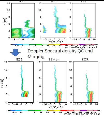
2.2.1. QC for Doppler Spectra

(i)

Deleting the data below the corresponding minimum range

The reflectivity in M3 with strong reflectivity detective ability is used to flag the saturation of M2 and M1 data according to their maximum reflectivity values in the range. When reflectivity is saturated, spectra are rejected from further processing. Echoes under the cloud bases detected by a laser ceilometer in the same site or Doppler spectral widths being less than 0.1 m·s⁻¹ are flagged as non-precipitation echoes.

(ii)

Dealiasing singly wrapped aliased Doppler spectral density algorithm based on the three types of spectra

Coherent integration numbers of 4 and 2 were used for M1 and M2 modes, and the Nyquist velocity was reduced to 4.635 m·s⁻¹ and 9.27 m·s⁻¹, respectively. In the presence of large droplets or strong airflows in convective systems, the Doppler spectra measured by M1 and M2 may be folded. However, the Nyquist velocity for M3 is 18.67 m·s⁻¹. The fall velocity of rain drops with a diameter of 6 mm at the ground is about 9.4 m·s⁻¹. Precipitation in a downdraft of 9.27 m·s⁻¹ can cause folded SZ3, which is apparently rare in real clouds and weak precipitation. The key to dealiasing Doppler spectra is to choose a reference radial velocity. The reference commonly used is from the dealiased values at a nearby gate under the assumption that the velocity within the cloud and precipitation is continuous. Errors are caused by either rapid sinking of hydrometeors or a strong updraft in the interior of a convective system. Therefore, a dealiasing algorithm based on Doppler spectra observed by M3 or M2 is proposed. Firstly, SZ3 is iteratively determined based on the folding type, and it is dealiased from the cloud top to base; then, the dealiased SZ3 is used as the reference Doppler velocity to determine the folding type in SZ2 dealiasing when these valid SZ3 observations are obtained in the sample bin. Finally, SZ1 is dealiased using the dealiased SZ3 and SZ2 as references.

(iii)

Detecting and removing artefacts produced by pulse compression in SZ2

To identify artefacts in the pulse-coded Doppler spectral data produced by M2, we used an algorithm similar in principle to that proposed by Moran et al. (1998) [1]. The difference is that Moran and coworkers removed artefacts from reflectivity data, whereas we removed the Doppler spectral bins contaminated by the range sidelobe, and retained only the uncontaminated spectral bins. The threshold T (dB) is calculated as follows:

$$-Rs-10.0·a{\log }_{10}(PCR)<T<-Rs,$$

(5)

where Rs is the range sidelobe for pulse compression, and PCR is the pulse compression ratio. For M2, Rs = −60 dB, PCR = 17.7 dB, and 42.3 dB < T < 60 dB.

Let SZ2(n, i) represent the Doppler spectral bin at the n-th FFT-bin in the i-th radar sample volume. The Doppler spectral bin SZ2(n, i) is flagged as possibly suffering from a range sidelobe if

$$SZ2(n,j)>SZ2(n,i)+T,$$

(6)

for any value of j that satisfies i − 21 < j < i + 21. The threshold T that identifies most range sidelobe artefacts is 60 dB. A threshold value of 42.3 dB eliminates the rare artefacts that are not identified by the 60-dB threshold.

2.2.2. Merging Algorithms for the Reflectivity Spectra Obtained Using the Three Operational Modes

1.

Principles of merging of the reflectivity spectra

The M1 mode has high sensitivity and velocity resolution for observing boundary layer clouds, which are often composed of small droplets. The M2 mode has the highest sensitivity among the modes and a large minimum range, enabling it to observe weakly reflective, high-altitude clouds. The M3 mode has large Nyquist velocity, large maximum reflectivity, and low minimum range, allowing observation of light precipitation. Large negative biases occur in reflectivity and reflectivity spectra at high Doppler velocities owing to the use of coherent integration in M2. An identical condition arises for the reflectivity spectra at low SNR for the M3 mode. V0 overestimated by the M3 mode and artefacts from pulse compression influence data applications. To develop a complete picture of the vertical distributions of hydrometeors and air speed, it is necessary to merge the reflectivity spectra from the three modes.

Some of the key issues in implementation of the merging process are as follows: (1) Doppler velocity aliasing and artefact and saturation removal must be performed before merging, and the data immune to these contaminations should be prioritized for usage to ensure data reliability. (2) SZ1 and SZ2 bins at low Doppler velocities (small particles) and low SNR should be used when SZ3 is underestimated; on the other hand, SZ3 should be used for higher Doppler velocities to avoid the negative biases introduced by coherent integration. (3) We should keep full spectral data by using SZ2. (4) The radial velocity resolution is the highest for the M1 mode and the lowest for the M3 mode. High-resolution data should be used when other parameters meet the requirements. (5) Measurement biases arising in different modes, especially for the M1 mode, should be taken into account. Reflectivity, radial velocity, and spectrum width should be calculated by merging the reflectivity spectra.

2.

Merging the reflectivity spectra

The steps for merging the reflectivity spectra are as follows:

(1)

The data below the defined SNR threshold and all of data below the corresponding minimum range are deleted.

(2)

The noise level is determined and all continuous spectral bins above the noise level with an SNR threshold and a bin-number threshold are picked up, as cloud signals typically have higher power and larger spectral width than noise. An objective method presented by Hildebrand and Sekhon is commonly used for millimeter-wave cloud radar studies [18]. However, a recent study argues that this approach can overestimate the radar noise power and, thus, it is not appropriate for solid-state cloud radars. In contrast, a segmental approach reported by Petitdidier et al. can achieve better accuracy and stability [19]. Hence, in this study, simple eight-segment technology was utilized to calculate radar noise level.

(3)

For merging the reflectivity spectra from SZ1, SZ2, and SZ3, we individually compare and evaluate the 256 reflectivity spectral bins of SZ1, SZ2, and SZ3, and choose the best bins to compose the newly merged reflectivity spectrum SZm. Aliasing and artefact flags for each spectral bin are used as the criteria to determine the spectra to be used. The amplitudes of the spectral bins are considered a key factor to avoid the influence of coherent integration and low SNR on the merged spectra.

Below the minimum range of the M2 mode, only SZ1 and SZ3 bins are available, whereas, above this range, we can use SZ1, SZ2, and SZ3 bins. If an SZ1 bin is flagged for aliasing, an SZ2 or SZ3 bin is used when available. If an SZ2 bin is flagged as an artefact, an SZ1 or SZ3 bin is used when available. If the SNR in M3 is less than 10 dB, SZ1 and SZ2 are used when available. In this case, SZ3 is unreliable. When there are two or three spectral bins from M1, M2, and M3 that are immune to these contaminations, the maximum value is chosen to reduce spectral underestimation resulting from coherent integration and low SNR. In some cases, only SZ1 or SZ2 points are available at the two ends of the spectra; then, SZ1 and SZ2 can be used to fill the gaps in SZ3, widen the spectra, and obtain accurate V0.

(4)

The reflectivity, radial velocity, and spectral width are recalculated from the merged reflectivity spectrum SZm.

$$Zm(R)={\displaystyle \sum _{i=1}^{n}SZm(i,R)\Delta V}$$

(7)

$$Vrm(R)=\frac{{\displaystyle \sum _{i=1}^n{V}_i·SZm(i,R)\Delta V}}{{\displaystyle \sum _{i=1}^{n}SZm(i,R)\Delta V}}$$

(8)

$$Swm(R)={\left[\frac{{\displaystyle \sum _{i=1}^n{(V_i-Vrm(R))}^2·SZm(i,R)\Delta V}}{{\displaystyle \sum _{i=1}^{n}SZm(i,R)\Delta V}}\right]}^{1/2}$$

(9)

Here, n = 256 is the number of FFT points; SZm (i, R) is the merged reflectivity spectra for the i-th FFT bin at the range gate of R; and Z_m, V_rm, and S_wm are the reflectivity, radial velocity, and spectral width, respectively.

3. Results

3.1. Doppler Spectral Evaluation and Effects of Observation Parameters in Different Operational Modes

For the Ka-band solid-state transmitter cloud radar, pulse compression and coherent integration techniques are used to improve the radar sensitivity and detection capability. However, for these techniques, the minimum range of useful data is wide; moreover, range sidelobe artefacts are introduced in the data, and the Nyquist velocity is reduced. These technologies also result in a bias in the Doppler spectra and their moments. The stratiform precipitation observed by the cloud radar on 4 June 2016 in southern China was used to analyze the consistencies of Doppler spectra, reflectivity, velocity, and spectrum width observed by the three work models. This stable stratiform precipitation case with medium strength, less spatio-temporal variations, and liquid and solid hydrometers introduced less effects of turbulence on the Doppler spectra and air vertical speed retrieval, and reduced the observation time effects on radar data from the three work modes. The radar data were suitable for analyzing the consistencies of Doppler spectra, and comparing the Doppler spectra for different phase hydrometers.

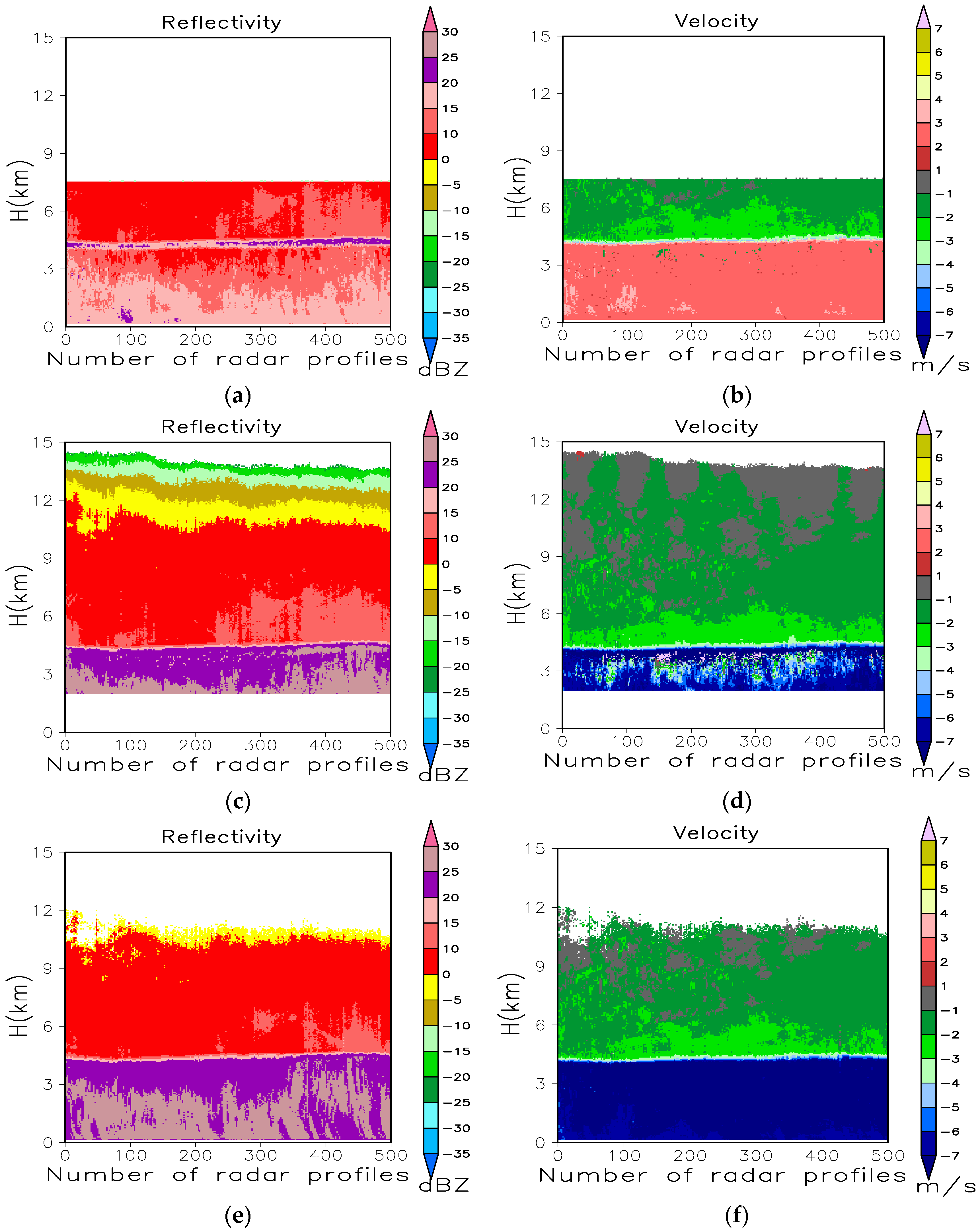
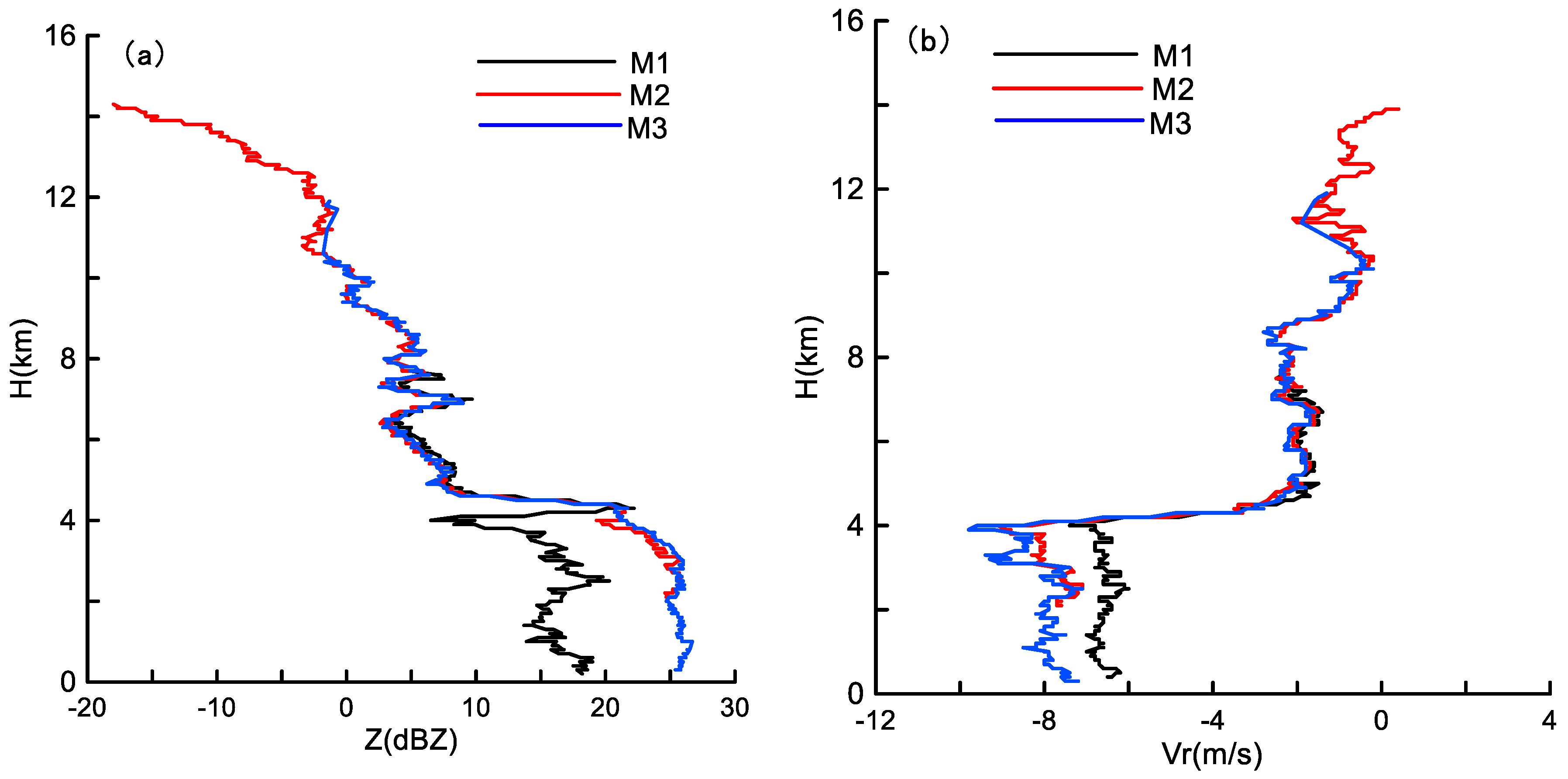
3.1.1. Consistency Analysis of Reflectivity and Velocity for the Three Modes

Figure 1 shows the time–height cross-sections of 500 profiles of raw reflectivity and radial velocity measurements obtained using the three modes for the period of 4:07 p.m. to 5:21 p.m. Beijing time (BT) on 4 June 2016. Since no pulse compression and coherent integration are performed for the M3 mode, the data from this mode are the least affected. Hence, we compared results for the other two modes with those for the M3 mode. The three modes captured similar reflectivity and velocity values above the bright band at a height of 4 km with low velocity values under −3.0 m·s⁻¹. Below the bright band at 4 km, velocity increased downward. Here, the velocity from the M3 mode was negative because of the falling of precipitation particles. A large proportion of these negative velocities exceeded the M1 Nyquist velocity of 4.67 m·s⁻¹. Note that the radial velocity obtained from the M1 mode and parts of velocity from M2 were simultaneously positive, indicating that the radial velocity was aliased. Four rounds of coherent integration in M1 resulted in a negative bias of reflectivity below the bright band when the radial velocity exceeded 4 m·s⁻¹. Two rounds of coherent integration in M2 had no obvious effects on reflectivity measurement. That is, the full of gain of coherent integration was not applicable for Doppler velocity, and a large Doppler velocity led to radar returns that decorrelated rapidly in time.

The reflectivity and dealiased velocity profiles obtained from the three modes for the 30th profile are shown in Figure 2. M1 underestimated the reflectivity by 6 dB. In other words, the gain of four rounds of coherent integration was nearly zero. Moreover, M1 underestimated the velocity by 1.5 m·s⁻¹, resulting in alteration of the Doppler spectral shapes. The facts indicate that four rounds of coherent integration not only attenuated reflectivity, but also changed the shape of Doppler spectra in the liquid precipitation region. However, two rounds of coherent integration deployed in M2 yielded full gain and had less of an effect on reflectivity and velocity. Note that CR was operated at PRF = 8333 Hz.

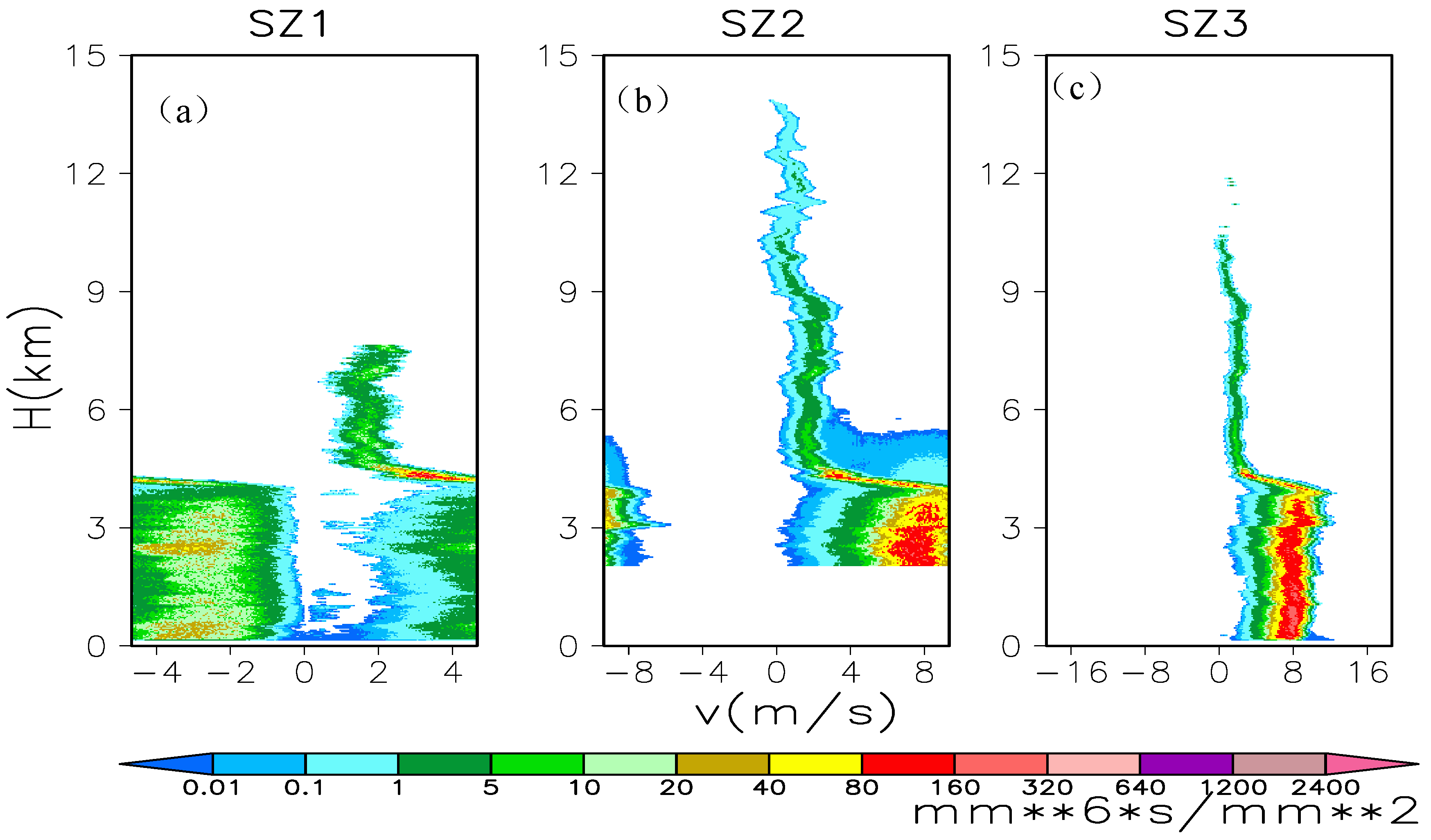
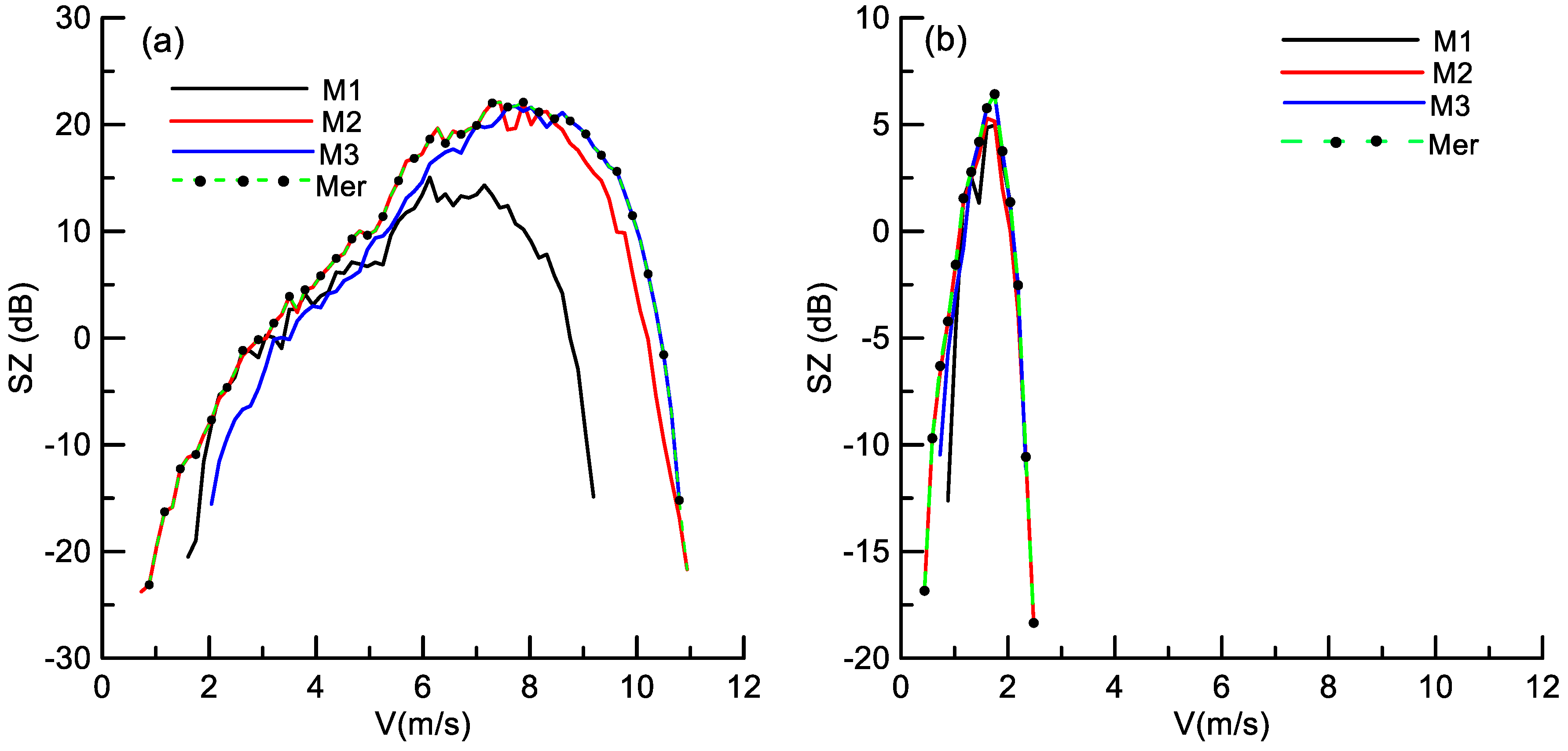
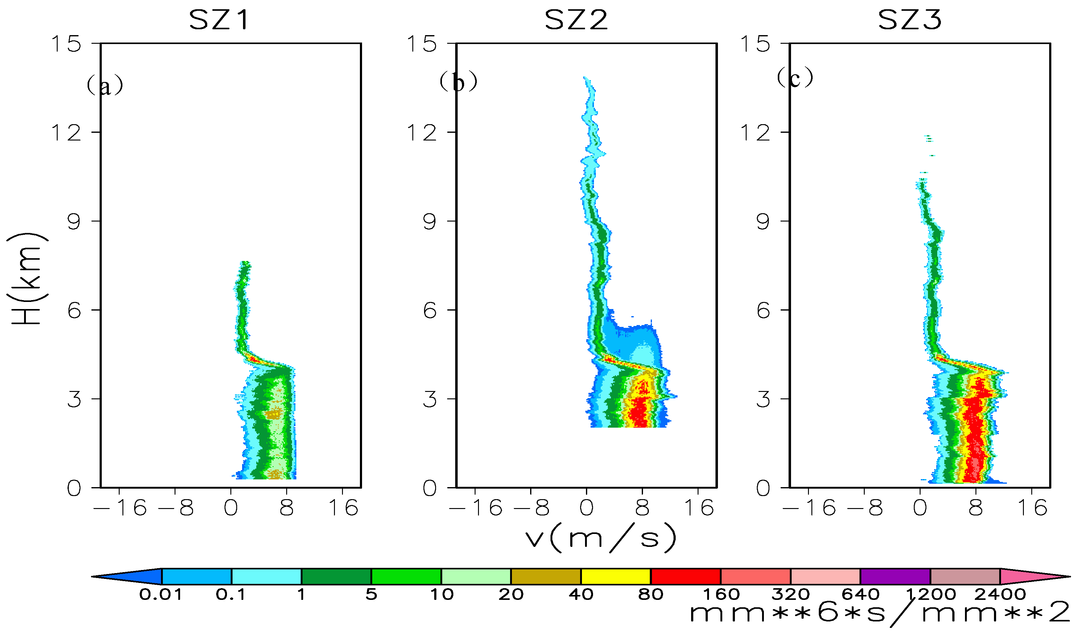
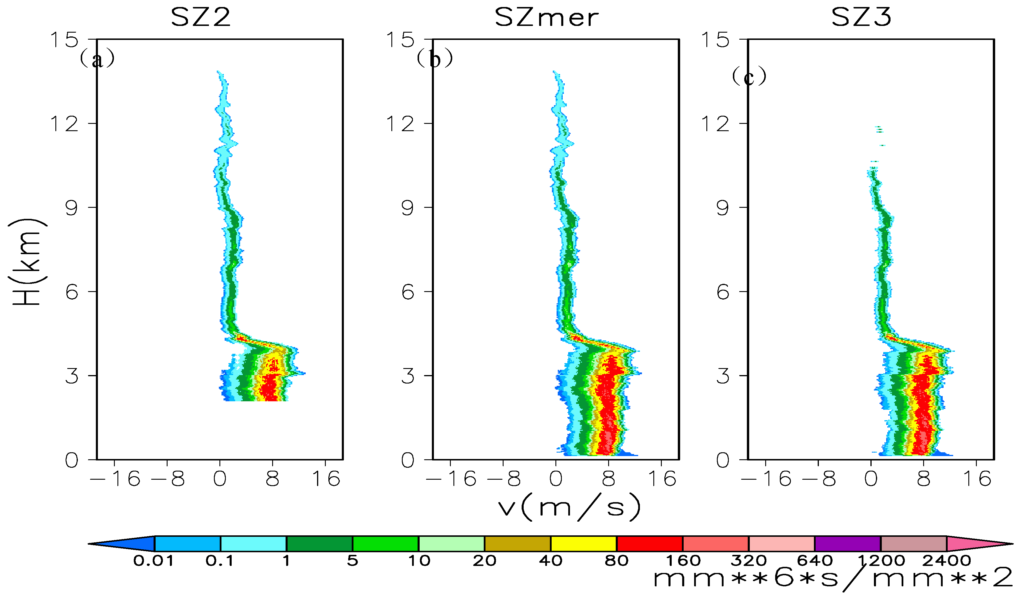
3.1.2. Consistency Analysis of Doppler Spectral Density for the Three Modes

To analyze the reasons for reflectivity and velocity biases in the three modes, the reflectivity spectral density from the three modes was examined. The reflectivity spectral density SZ (mm⁵·m⁻³·s) is calculated from the Doppler spectral density SP as follows:

$$SZ(i,j)=\frac{Z·SP(i,j)}{{\displaystyle \sum _{i=1}^{n}SP(i,j)\Delta V}},$$

(10)

where SZ(i, j ) and SP (i, j) are the reflectivity and Doppler spectral density at the i-th FFT bin and j-th range gate, respectively. Z is the reflectivity, ΔV is the velocity resolution, and n = 256 is the number of FFT points.

Figure 3 shows the reflectivity spectra across different heights for the 30th profile. Positive velocities are downward. The reflectivity spectra for solid precipitation above a height of 4 km were narrow. In the bright band (3.8–4.9 km), the spectra of solid hydrometeors were widened by the melting process; this resulted in wrapped aliased Doppler spectra SZ1 and SZ2 for liquid hydrometeors. For SZ2, the range sidelobe of SZ2 points for larger Doppler velocities produced by liquid hydrometers appeared between 3.9 and 5.7 km. The values of SZ1 for Doppler velocity >6 m·s⁻¹ were lower than those of SZ2 and SZ3. The parts of the Doppler spectra in liquid hydrometeors below 4.0 km exceeded the maximum velocities of M1 and M2, and were aliased to the left side (Figure 3a,b).

Coherent integration not only reduced the Nyquist velocity, but also underestimated the reflectivity spectra. Figure 4 shows the dealiased SZ1 and SZ2 and raw SZ3 for liquid hydrometeors at 2.7 km and solid hydrometeors at 6.6 km. Four rounds of coherent integration resulted in a bias of about −10 dB in SZ1 for V > 6 m·s⁻¹. When V > 10 m·s⁻¹, SZ2 was weaker than SZ3 by 2 dB. For solid hydrometeors, when the Doppler velocity was less than 3 m·s⁻¹, all three reflectivity spectra were similar. The obvious left shifts of the spectra were probably due to the microscale updraft.

The minimum detectable reflectivities of M1 and M2 were less than the value for M3 by 6 dB and 20.8 dB, respectively. The different minimum detectable reflectivities resulted in SZ1, SZ2, and SZ3 of different widths and Doppler velocities for the first valid left endpoint (V0). For hydrometeors, V0 was 1.8, 0.95, and 2.12 m·s⁻¹ for SZ1, SZ2, and SZ3, respectively. If the effects of turbulence on the spectra were negligible, the vertical speeds of air retrieved by SZ1, SZ2, and SZ3 were −1.8, −0.95, and −2.12 m·s⁻¹, respectively. Positive air vertical velocities are upward. Also, the SZ on the left side was underestimated by M3 for low signal-to-noise ratio (SNR).

The spectral data observed on 4 June 2016 were used to statistically analyze the averaged bias between SZ1 and SZ3 and between SZ2 and SZ3 for different Doppler velocity values (or FFT bins) (Figure 5). From the averaged SZ3, we can see that SZ3 had two peaks—one had a small scope and was from hydrometeors with slow fall speed, while the other had a large scope and was from hydrometeors with fast fall speed. Most of the spectral points with V < 4.0 m·s⁻¹ were attributed to solid hydrometeors, whereas others were attributed to small liquid hydrometeors, because solid hydrometeors and small liquid hydrometeors have small fall velocities and their return power is low. Since the variational patterns of the averaged bias and SZ3 with Doppler velocity are opposite, we deduced that the overestimation of the reflectivity spectra for V < 2.0 m·s⁻¹ by M1 and M2 mainly resulted from the differences in SNR between M1 and M3. Underestimations of the reflectivity spectra for V > 2.0 m·s⁻¹ by M1 and for V > 8.0 m·s⁻¹ by M2 resulted from coherent integration. The underestimations of reflectivity by M1 for liquid precipitation were attributed to the underestimations of spectra with larger Doppler velocities, which also produced biases in the radial velocity and spectral width measurements.

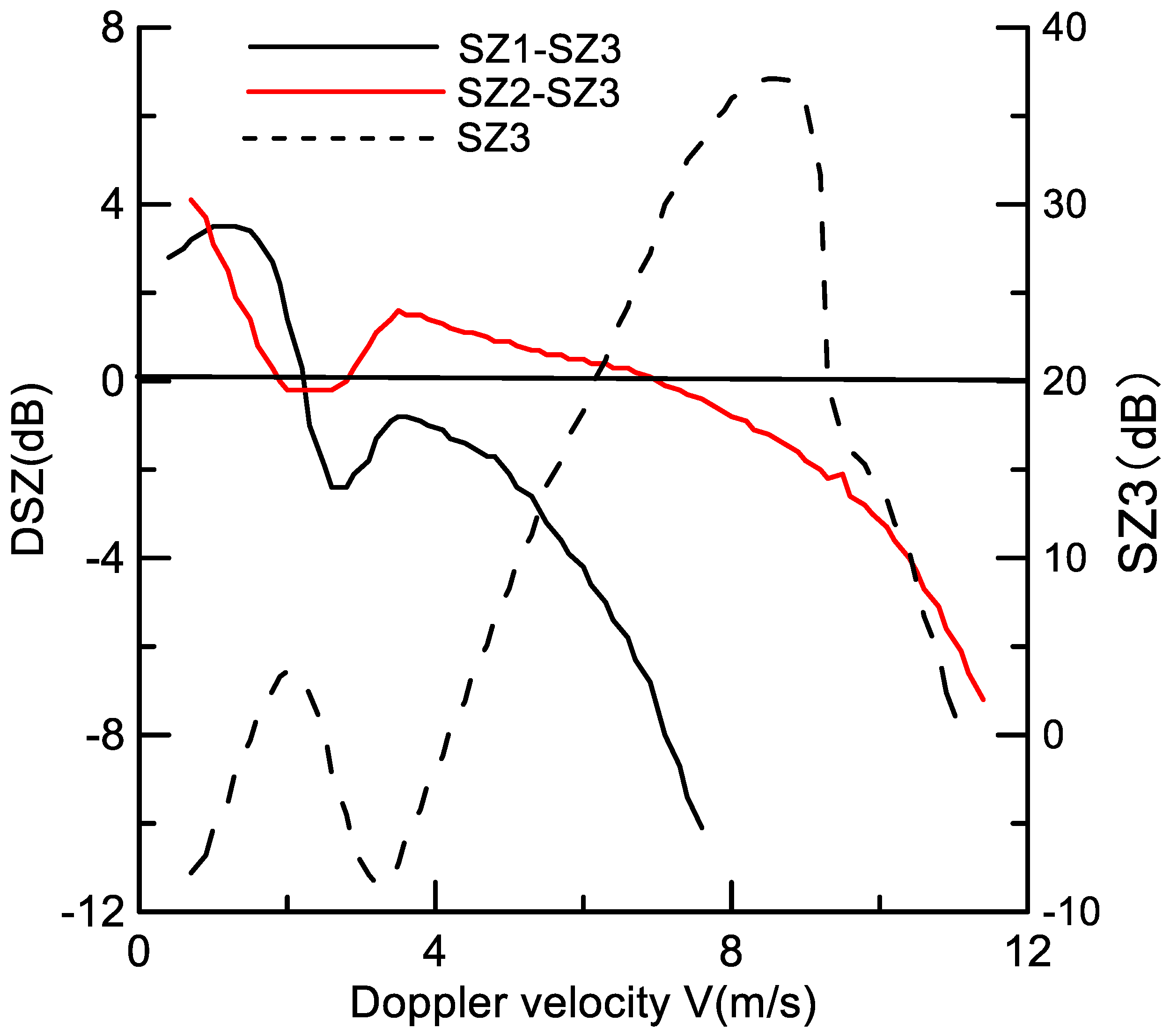
3.1.3. Pulse Compression Effects on SZ2

Figure 6a shows SZ1, SZ2, and SZ3 for solid hydrometeors at 4.5 km, located at the top of the bright band. M1 and M2 modes could only observe spectra for Doppler velocities less than 4 m·s⁻¹; therefore, the SZ2 for V > 5 m·s⁻¹ was from the range sidelobe for big liquid hydrometeors below 4.0 km. Figure 6b shows the vertical profiles of SZ2 points at 5, 240, and 250 FFT points, and the Doppler velocities for the three FFT points were 9.79, 8.156, and 8.88 m·s⁻¹, respectively. The SZ2 points had different values between 3.9 and 5.7 km. Figure 3 shows that the Doppler velocity did not exceed 6 m·s⁻¹ above 3.9 km in any spectrum. The three SZ2 points above 3.9 km were range sidelobe artefacts from the hydrometeors below this level. The variations in the SZ points with altitude depended on the number of radar bins of range sidelobes that contributed to the artefacts. For example, only one sidelobe contributed to SZ2 at 5.7 km, whereas 60 sidelobes contributed in the case of SZ2 at 4.2 km. The difference between SZ2 points of the range sidelobe at 5.7 km and the main lobe at 3.9 km was 56 dB; this difference was consistent with fact that the range sidelobe of pulse compression was −60 dB. This difference was 39 dB for SZ2 points between 4.2 km and 3.9 km. The difference between the range sidelobe of SZ2 at 5.7 km and 4.2 km was 17 dB, which was consistent with the gain of 17.7 dB attributed to pulse compression in M2.

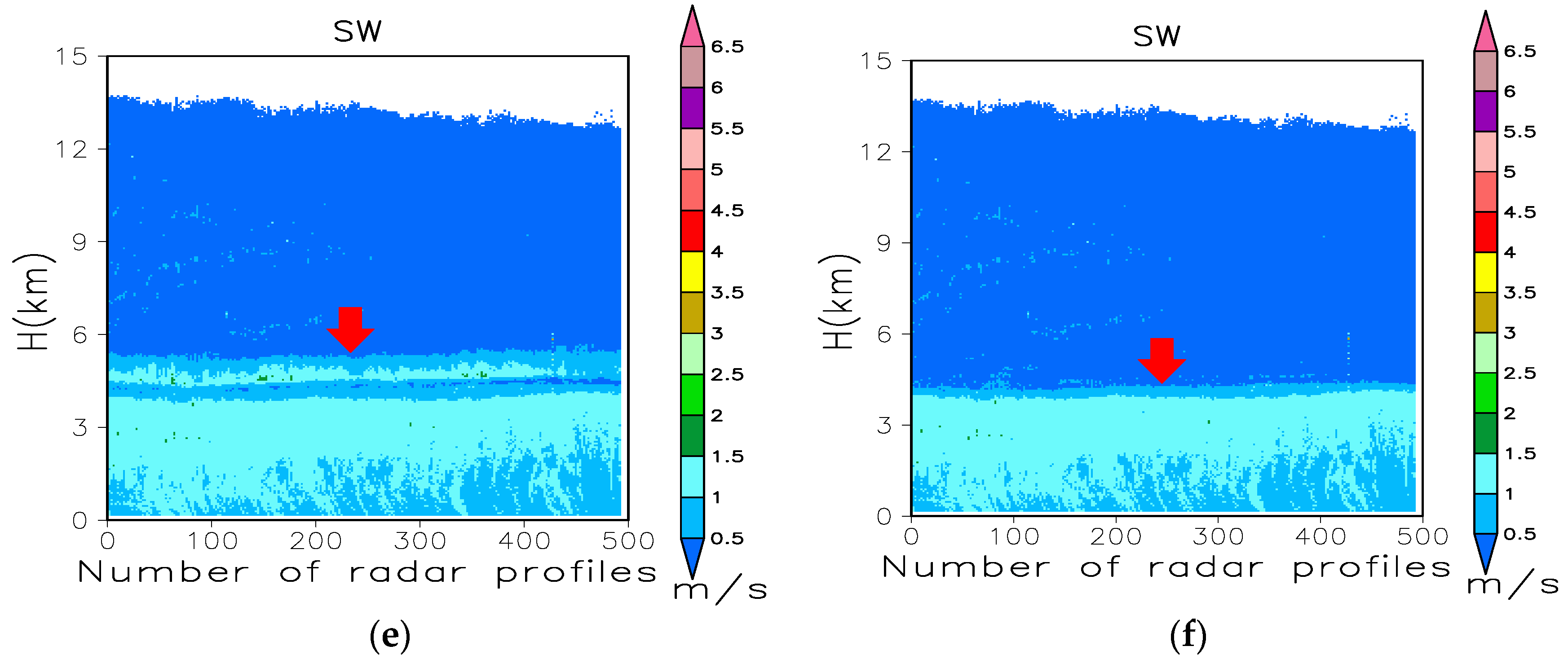
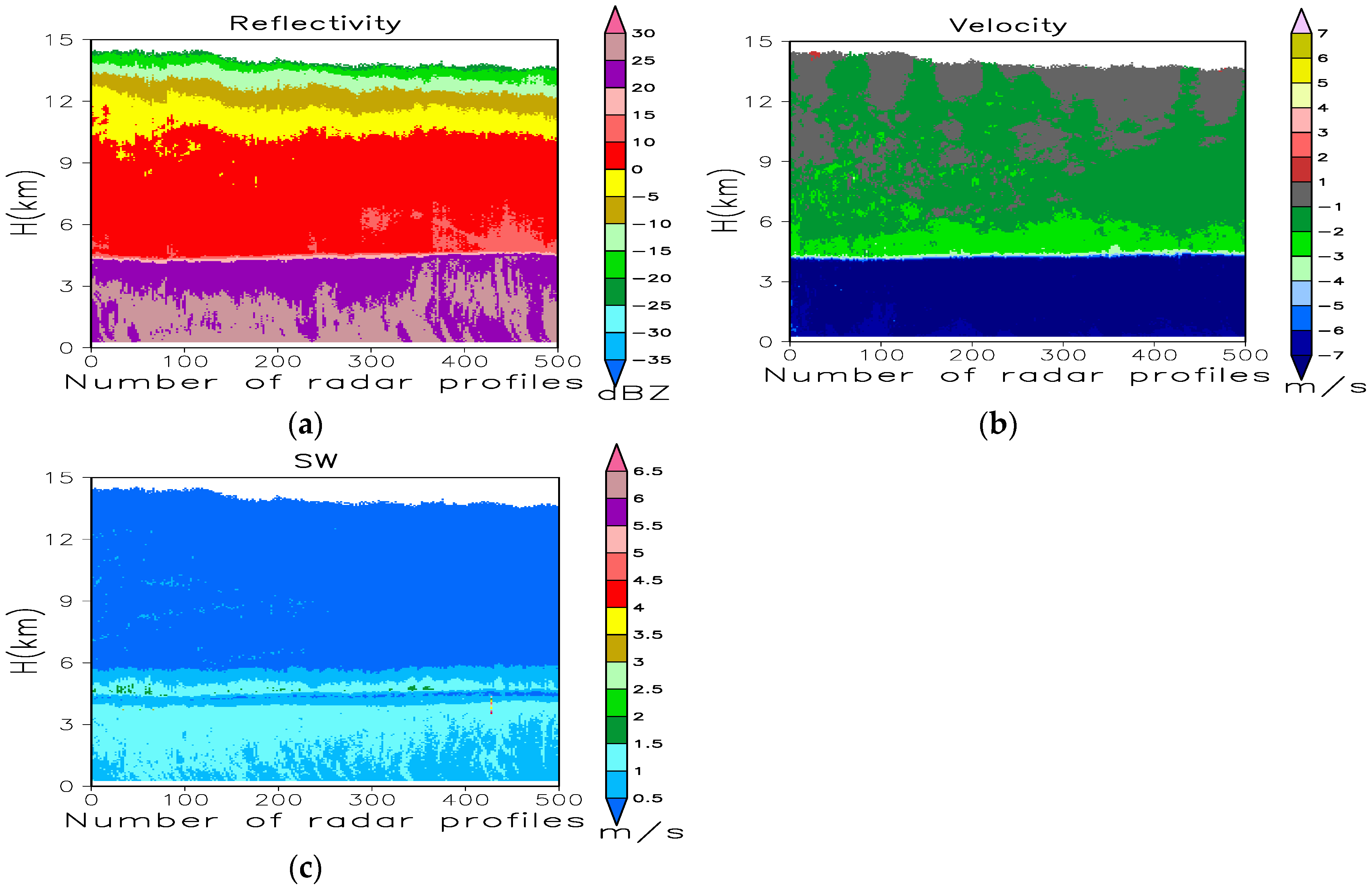
3.2. SZ Quality Control and Merging Result

Figure 7 shows a comparison of the dealiased SZ1 and SZ2 with SZ3; their raw data are shown in Figure 3. Figure 8 shows SZ2 after removing artefacts and the merged spectrum SZm. The aliasing of SZ1 and SZ2 below 4 km was addressed correctly, but the SZ1 below 0.5 km could not be recovered, because valid spectra were full with 256 points; thus, we could not determine which points were aliased. A comparison of Figure 7b and Figure 8b indicates that the artefacts in solid hydrometeor Doppler spectra were removed, and the Doppler spectra from solid hydrometeors were reserved. The algorithm proposed by Moran et al. (1998), based on the non-range-corrected return power [1], failed to remove the artefacts. This was because the average difference in return power between 3.9 and 5.7 km and between 3.6 and 1.8 km was about 20 dB, which was less than the threshold T in Equation (3). In this case, the contributions of the artefacts to reflectivity were not obvious, but its contributions to velocity and spectral width were not negligible. Using the Doppler spectra, we not only removed the artefacts in the SZ2 bins, but also retained the uncontaminated SZ2 bins, which were used to correct and recalculate the reflectivity, velocity, and spectral width.

Upon comparing SZm with SZ1, SZ2 and SZ3, we can see that SZm filled in the gaps in SZ3 during weak cloud periods above 10 km and reduced the effects of coherent integration and pulse compression on SZ1 and SZ2 in liquid precipitation below 4 km. Meanwhile, the merging of reflectivity spectra with different Nyquist velocities and resolutions reduced velocity folding and provided finer information about cloud and precipitation dynamics.

From SZm at 2.7 and 4.5 km shown in Figure 4, we can see that the SZm bins originated from SZ2 at low (0.5 m·s⁻¹ ≤ V ≤ 8 m·s⁻¹) and from SZ3 for high (V > 8 m·s⁻¹) Doppler velocities for liquid precipitation, while SZ1 did not contribute to SZm. In this case, the spectra with large velocity were underestimated. For weak cloud and precipitation below 2.1 km and solid cloud, SZ1 was used to produce SZm.

In order to explain the contaminations of range sidelobe artefacts on the three moments of Doppler spectra, Figure 9 presents comparisons between the recalculated reflectivity, radial velocity, and spectrum width obtained only after dealiasing, and the corresponding results obtained after dealiasing and artefact removal from SZ2. Their raw data are shown in Figure 1. The pulse compression sidelobe produced a band with a larger spectrum width above the bright band (Figure 9e; removed in Figure 9f marked by red arrows). The pulse compression sidelobe also introduced some error in the radial velocity measurement. The Doppler spectra QC successfully removed these contaminations. The merged reflectivity below the bright band was from SZ3, which resolved the reflectivity underestimations by M1 and M2 (Figure 1a,e and Figure 9b). The merged three moments of Doppler spectra had high quality.

In order to reveal the advantage of Doppler spectra QC and merging, Figure 10 shows the merged reflectivity, velocity, and spectral width from raw data, compared with the previous merging algorithm proposed by Liu [15]. For merged data in Figure 10, after systematic bias correction of reflectivity, and removal of the range sidelobe artefacts using non-range-corrected return power, the data were merged considering radial velocity aliasing and reflectivity saturation from M1 and M2, and radial velocity resolutions. Figure 10 is similar to Figure 9a,c,d, which were merged only after dealiasing using the new algorithm. In fact, the previous algorithm failed to remove the range sidelobe artefacts, which were resolved using the new algorithm. However, we conducted Doppler spectra QC to remove velocity aliasing and range sidelobe artefacts, then produced the merged Doppler spectra, and recalculated the three moments of Doppler spectra in Figure 9. The new algorithm resolved the reflectivity underestimated due to coherent integration (Figure 9a and Figure 10a), and resolved the range sidelobe artefact contamination’s effect on reflectivity and spectral width over the bright band (Figure 9d,f and Figure 10b,c). Upon comparing the previous merged algorithm, the key improvements of the new algorithm involve a removal of the range sidelobe artefact contamination on reflectivity and spectral width, and a dealiasing of the velocity by M1 and M2.

In order to explain the structures, Figure 11 shows the recalculated reflectivity, velocity, and spectral width profiles for modes M1, M2, and M3 and the merging results from SZm. A comparison of the merged reflectivity and radial velocity with the raw data for modes M1, M2, and M3 shows that M1 underestimated reflectivity by about 9 dBZ and velocity by about 1.5 m/s in the liquid precipitation area. We can find obvious range sidelobe contaminations of spectral width of M2, which were removed from the merged data by the SZ QC (Figure 11c). Doppler spectra QC aliased the SZ1 and SZ2 and removed the range sidelobe contaminations. More cloud and precipitation were detected by the merged reflectivity, especially for weak clouds and heavy precipitation, than by a single mode. The underestimated reflectivity by M1 was recovered. Velocity aliasing was not observed in the merged velocity.

4. Discussion

Now, we discuss the effects of V0 on the retrieved raindrop size distribution (DSD). For convenience, we neglect the spectral broadening caused by turbulence and wind shear. Furthermore, if small particles, which are regarded as tracers of clear-air motions in the measured spectra, are present within the cloud radar sampling volume, the vertical air velocity can be directly estimated using the velocity bin of these small targets. In this case, the DSD is retrieved from the reflectivity spectrum [8]. The algorithm described in Reference [11] was used to analyze the DSD in stratiform precipitation. The DSD was retrieved using Equation (11).

$$\mathrm{S}Z(Vr-V0)=\frac{{10}^6{\lambda }^4}{{\pi }^5}\frac{{\left|\epsilon +2\right|}^2}{{\left|\epsilon -1\right|}^2}\mathrm{N}\left(\mathrm{D}\right(\mathrm{Vr}\text{-}\mathrm{V}\left)\right)·\sigma (D(\mathrm{Vr}\text{-}\mathrm{V}0))\frac{\partial D}{\partial V_f},$$

(11)

where SZ(Vr-V0) is the reflectivity spectrum shifted with V0, N(D) is the raindrop size distribution, λ is the wavelength, σ(D) is the backscattering cross-section, and Vf is the fall speed of a raindrop. The rain rate R (mm·h⁻¹), liquid water content LWC (g·m⁻³), total number density Na (m⁻³), and average diameter Dm (mm) from the retrieved DSD are calculated as follows:

$$R=\frac{\pi }{6}{\displaystyle \sum _{i=1}^n{D}_i{}^3·V_f{}_i(D_i)·N(D_i)\Delta D_i};$$

(12)

$$LWC=\frac{\pi }{6}{\displaystyle \sum _{i=1}^n\rho ·D_i{}^3·N(D_i)\Delta D_i};$$

(13)

$$N_a={\displaystyle \sum _{i=1}^{n}N(D_i)\Delta D_i};$$

(14)

$$Dm={\left(\frac{{\displaystyle \sum _{i=1}^n{D}_i{}^3·N(D_i)\Delta D_i}}{N_a}\right)}^{1/3}.$$

(15)

We conducted three experiments to investigate the influences of V0 and the three work modes on the retrieved DSDs. Considering the high sensitivity of M2, the V0 in M2 and SZ3 were regarded as “truths”. In experiment 1 (T1), we used V0 from M2 for all reflectivity spectra, and the results from SZ3 as “truths.” In experiment 2 (T2), the three V0 observed by M1, M2, and M3 were used in SZ1, SZ2, and SZ3, respectively. T2 was used in real CR data analysis. In experiment 3 (T3), we assumed V0 = 0 for all three spectra. That is, we neglected air vertical motion, which is considered for DSD retrieval in the case of the micro-rain radar. According to the retrieval algorithm, reflectivity only affects the number density, whereas V0 and the shape of the reflectivity spectra affect the width, shape, and average diameter of DSD.

Figure 12 shows SZ1, SZ2, and SZ3 after being shifted by V0 at the radar range gate of 90, and the DSD retrieved from the three experiments.

Table 3. Microphysical parameters retrieved in the three experiments. R—rain rate; LWC—liquid water content; Na—total number density; Dm—average diameter.

Work Mode	Experiment	Z (dBZ)	V0 (m·s−1)	R (mm·h−1)	LWC (g·m−3)	Na (m−3)	Dm (mm)
M1	T1	17.8	0.95	0.39	0.029	449	1.01
	T2	17.8	1.8	0.67	0.065	3144	0.67
	T3	17.8	0	0.21	0.012	42	1.63
M2	T1	25.6	0.95	1.33	0.07	787	1.13
	T2	25.6	0.95	1.33	0.07	787	1.13
	T3	25.6	0	0.85	0.038	96	1.8
M3	T1	25.0	0.95	1.01	0.05	196	1.59
	T2	25.0	2.12	2.04	0.145	2629	0.94
	T3	25.0	0	0.87	0.03	26	2.6

lists the retrieved rain rate R (mm·h⁻¹), liquid water content LWC (g·m⁻³), total number density Na (m⁻³), and average diameter Dm (mm) from the retrieved DSD.

A comparison of T2 with “truth” DSD (SZ3 in T1) shows that, in the real retrieved DSD (T2), SZ1 underestimated the DSD and other parameters mainly because of coherent integration; SZ2 underestimated the number concentration of big raindrops and overestimated that of small drops; and SZ3 yielded results similar to those of SZ2 because of the positive bias of V0.

A comparison of T1 with T3 shows the effects of negation of air motion on the DSD (Figure 11a,b,e,f). In this case, a downdraft was observed. SZ1, SZ2, and SZ3 were shifted to the left by 0.98 m·s⁻¹ in T1, whereas they remained unchanged in T3. Furthermore, in T3, Na, LWC, and R were underestimated, and Dm is overestimated. If the updraft of air motion was neglected, Na, LWC, and R were overestimated, and Dm was underestimated.

A comparison of SZ1 and SZ3 with SZ2 shows that V0 for SZ1 and SZ3 was underestimated by 0.32 and 1.17 m·s⁻¹, respectively, resulting in a leftward shift of SZ1 and SZ3 in T1. Na, LWC, and R from SZ1 and SZ3 were overestimated, and Dm was underestimated in T2. That is, the low-sensitivity modes such as M1 and M3 underestimated V0, resulting in the overestimation of Na, LWC, and R.

Compared with the M3 mode, four rounds of coherent integration (the number of coherent integrations was four) were performed for the M1 mode to boost radar sensitivity, and the minimum detectable reflectivity decreased by 6 dB (10.0 × log₁₀ (4)). Similarly, two rounds of coherent integration were performed for the M2 mode, and the pulse compression ratio was 60. Theoretically, the minimum detectable reflectivity could be reduced by 20.8 dB (10.0*log₁₀ (2*60). M1 and M2 underestimated V0 by 0.32 and 1.17 m·s⁻¹, respectively, due to the extension of the reflectivity spectra and the leftward shift of V0. The leftward shift of V0 increased the corresponding velocity of SZ1 and overestimated the average diameters. M1 also underestimated the reflectivity and SZ1 for larger Doppler velocities, which underestimated the number of larger raindrops. The observation obtained from M1 underestimated Na, LWC, R, and Dm. In the case of S2, Na, LWC, and R were underestimated, and Dm was overestimated (Figure 7c,d).

5. Conclusions

The Chinese Ka-band solid-state transmitter cloud radar can operate in three work modes (M1, M2, and M3) with different pulse widths and coherent integration and non-coherent integration numbers to meet the requirements for long-term cloud measurements and observations of weak cloud. The CR observation data in southern China were used to analyze the consistencies of the reflectivity spectra obtained using the three modes, and to examine the influence of coherent integration and pulse compression on the retained data. Algorithms for Doppler spectral density data QC and merging were proposed herein in order to remove the effects of pulse compression and coherent integration on Doppler spectra and their moments, and to yield a comprehensive and accurate depiction of most of the clouds and precipitation in the vertical column above the radar. These algorithms were based on multiple-mode observation data. After dealiasing Doppler velocity and artefact removal, three types of Doppler spectral density data were merged. The Doppler moments, namely, reflectivity, radial velocity, and spectral width, were recalculated from the merged reflectivity spectra. The performance of the merging algorithm was evaluated. The major conclusions are as follows:

(i)

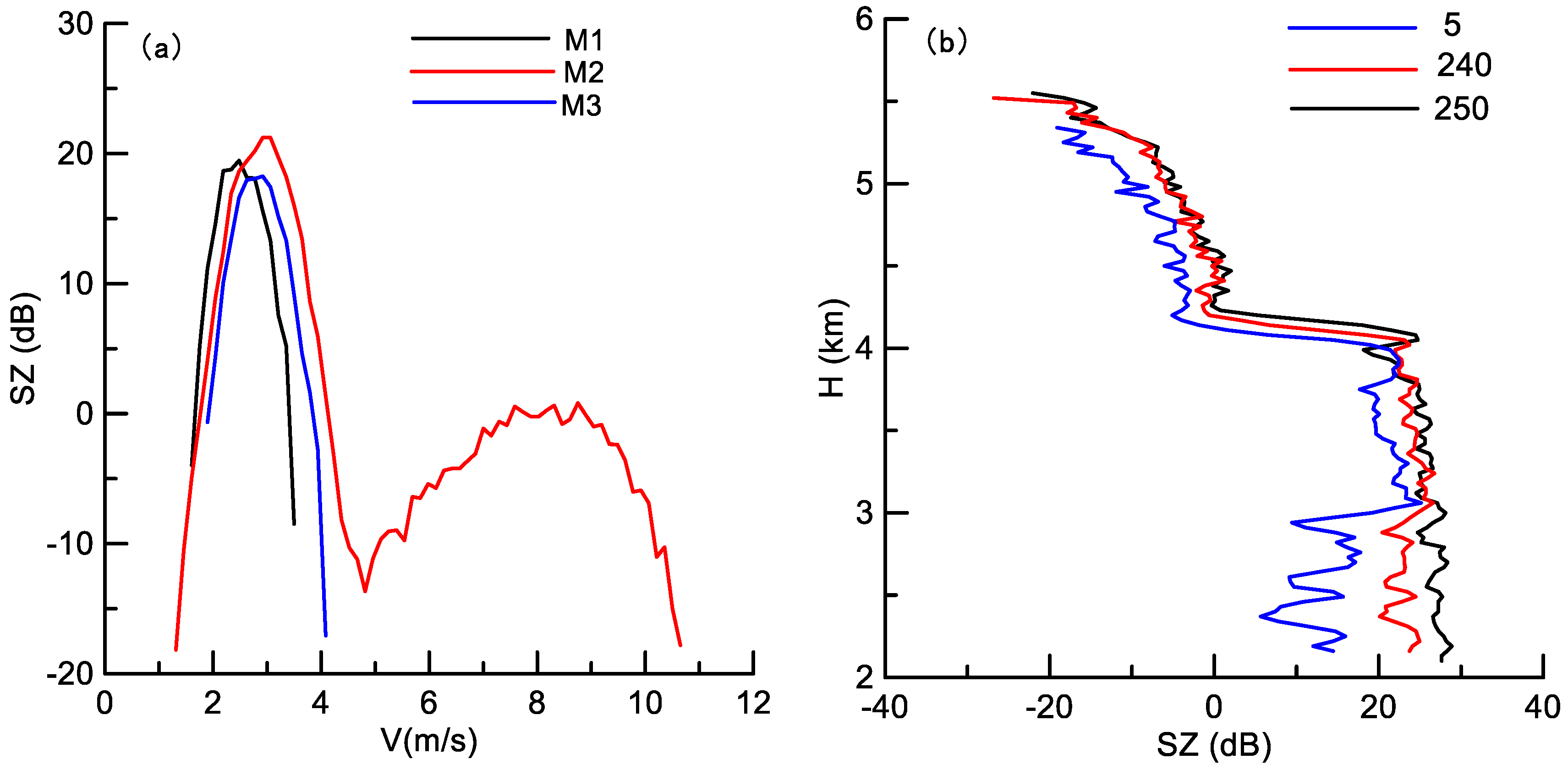
In mode M1, four rounds of coherent integration with a PRF of 8333 Hz underestimated the reflectivity spectra for Doppler velocities exceeding 2 m·s⁻¹. This resulted in a large negative bias in the reflectivity and radial velocity when large drops were present. The reflectivity spectra were underestimated by mode M3 at low SNR. Additionally, two rounds of coherent integration in M2 had less of an effect on the reflectivity spectra.

(ii)

Pulse compression in M2 improved the radar sensitivity and air vertical speed observation, whereas M3 overestimated V0. This resulted in an underestimation of the number of big drops and an overestimation of the number of small drops. The number of larger drops was underestimated by M1.

(iii)

A comparison of the three individual spectra from modes M1, M2, and M3 showed that the merged reflectivity spectra filled in the gaps during weak cloud periods, reduced the effects of coherent integration and pulse compression in liquid precipitation, mitigated the aliasing of Doppler velocity, and removed the artefacts. The range sidelobe produced by pulse compression could be easily removed from the Doppler spectral density data than from the reflectivity data.

(iv)

The reflectivity, radial velocity, and spectral width recalculated from the merged reflectivity spectra were immune to the effects of coherent integration and pulse compression, and were consistent for clouds and weak and intermediate precipitation.

References

1. Moran, K.P.; Martner, B.E.; Post, M.J.; Kropfli, R.A.; Welsh, D.C.; Widener, K.B. An unattended cloud-profiling radar for use in climate research. Bull. Am. Meteorol. Soc. 1998, 79, 443–455. [Google Scholar] [CrossRef]
2. Clothiaux, E.E.; Moran, K.P.; Martner, B.E.; Ackerman, T.P.; Mace, G.G.; Uttal, T.; Mather, J.H.; Widener, K.B.; Miller, M.A.; Rodriguez, D.J. The Atmospheric Radiation Measurement Program Cloud Radars: Operational Modes. J. Atmos. Ocean. Technol. 1999, 16, 819–827. [Google Scholar] [CrossRef]
3. Schmidt, G.; Ruster, R.; Czechowsky, P. Complementary code and digital filtering for detection of weak VHF radar signals from the mesosphere. IEEE Trans. Geosci. Electron. 1979, 17, 154–161. [Google Scholar] [CrossRef]
4. Clothiaux, E.E.; Thomas, P.A.; Mace, G.G.; Moran, K.P.; Marchand, R.T.; Miller, M.A.; Martner, B.E. Objective Determination of Cloud Heights and Radar Reflectivities Using a Combination of Active Remote Sensors at the ARM CART Sites. J. Appl. Meteorol. 2000, 39, 645–665. [Google Scholar] [CrossRef]
5. Kollias, P.; Clothiaus, E.E.; Miller, M.A.; Luke, E.P.; Johnson, K.L.; Moran, K.P.; Widener, K.B.; Albrecht, B.A. The atmospheric radiation measurement program cloud profiling radars: Second-generation sampling stratrgies, processing and cloud data products. J. Atmos. Ocean. Technol. 2007, 24, 1119–1214. [Google Scholar] [CrossRef]
6. Sokol, Z.; Minářová, J.; Novák, P. Classification of Hydrometeors Using Measurements of the Ka-Band Cloud Radar Installed at the Milešovka Mountain (Central Europe). Remote Sens. 2018, 10, 1674. [Google Scholar] [CrossRef]
7. Lhermitte, R. Observations of rain at vertical incidence with a 94 GHz Doppler radar: An insight of Mie scattering. Geophys. Res. Lett. 1988, 15, 1125–1128. [Google Scholar] [CrossRef]
8. Kollias, P.; Albrecht, B.A.; Marks, F.D., Jr. Cloud radar observations of vertical drafts and microphysics in convective rain. J. Geophys. Res. 2003, 108, 40–53. [Google Scholar] [CrossRef]
9. Gossard, E.E.; Strauch, R.G. Measurement of cloud droplet size spectra by Doppler radar. J. Atmos. Ocean. Technol. 1994, 11, 712–726. [Google Scholar] [CrossRef]
10. Kollias, P.; Albrecht, B.A.; Lhermitte, R.; Savtchenko, A. Radar observations of updrafts, downdrafts, and turbulence in fair weather cumuli. J. Atmos. Sci. 2001, 58, 1750–1766. [Google Scholar] [CrossRef]
11. Shupe, M.D.; Kollias, P.; Matrosov, S.Y.; Schneider, T.L. Deriving mixed-phase cloud properties from Doppler radar spectra. J. Atmos. Ocean. Technol. 2004, 21, 660–670. [Google Scholar] [CrossRef]
12. Shupe, M.D.; Koliias, P.; Matrosov, M.; Eloranta, E. On deriving vertical air motions from cloud radar Doppler spectra. J. Atmos. Ocean. Technol. 2008, 25, 547–557. [Google Scholar] [CrossRef]
13. Liu, L.P.; Xie, L.; Cui, Z.; Li, X. The examination and application of Doppler spectral density data in drop size distribution retrieval in weak precipitation by cloud radar. Atmos. Phys. 2014, 38, 223–236. (In Chinese) [Google Scholar]
14. Liu, L.P.; Zheng, J.F.; Ruan, Z.; Hu, Z.Q.; Cui, Z.H. Comprehensive Radar Observations of Clouds and Precipitation over the Tibetan Plateau and Preliminary Analysis of Cloud Properties. J. Meteorol. Res. 2015, 29, 546–561. [Google Scholar] [CrossRef]
15. Liu, L.P.; Zheng, J.F.; Wu, J.Y. A Ka-band solid-state transmitter cloud radar and data merging algorithm for its measurements. Adv. Atmos. Sci. 2017, 34, 545–558. [Google Scholar] [CrossRef]
16. Zheng, J.F.; Liu, L.P.; Zhu, K.Y.; Wu, J.Y.; Wang, B.Y. A Method for Retrieving Vertical Air Velocities in Convective Clouds over the Tibetan Plateau from TIPEX-III Cloud Radar Doppler Spectra. Remote Sens. 2017, 9, 964. [Google Scholar] [CrossRef]
17. Kollias, P.; Albrecht, B.A.; Clothiaux, E.E.; Miller, M.A.; Johnson, K.L.; Moran, K.P. The Atmospheric Radiation Measurement Program Cloud Profiling Radars: An Evaluation of Signal Processing and Sampling Strategies. J. Atmos. Ocean. Technol. 2005, 22, 930–948. [Google Scholar] [CrossRef]
18. Hildebrand, P.H.; Sekhon, R.S. Objective determination of the noise level in Doppler spectra. J. Appl. Meteorol. 1974, 13, 808–811. [Google Scholar] [CrossRef]
19. Petitdidier, M.; Sy, A.; Garrouste, A.; Delcourt, J. Statistical characteristics of the noise power spectral density in UHF and VHF wind profilers. Radio Sci. 1997, 32, 1229–1247. [Google Scholar] [CrossRef] [Green Version]
Figure 1. Time–height cross-sections of raw reflectivity and radial velocity measurements from (a,b) M1, (c,d) M2, and (e,f) M3 for 500 radar profiles for the period between 4:07 p.m. and 5:21 p.m. Beijing time (BT) on 4 June 2016. The height is given above ground level. The reflectivity below 4.5 km is underestimated by M1 in (a), while the velocities in (b) and (d) are aliased.
Remotesensing 11 00209 g001
Figure 2. (a) Reflectivity and (b) dealiased velocity profiles obtained from the three modes for the 30th profile.
Remotesensing 11 00209 g002
Figure 3. Reflectivity spectra across different heights for the 30th profile observed by (a) M1, (b) M2, and (c) M3. Positive velocities are downward. The left sides of the spectra are aliased in SZ1 and SZ2. Note that there are different maximum velocities for the three work models.
Remotesensing 11 00209 g003
Figure 4. SZ1, SZ2, and SZ3 for (a) liquid hydrometeors at 2.7 km, and (b) solid hydrometeors at 6.6 km. The merged reflectivity and velocity (marked with “Mer”) is also shown.
Remotesensing 11 00209 g004
Figure 5. Variations in the averaged bias of the reflectivity spectra with Doppler velocity between SZ1 and SZ3 and between SZ2 and SZ3. The averaged SZ3 is also shown.
Remotesensing 11 00209 g005
Figure 6. (a) SZ1, SZ2, and SZ3 for solid hydrometeors at 4.5 km, and (b) vertical profiles of SZ2 points at 5, 240, and 250 fast Fourier transform (FFT) points, produced by the liquid hydrometeor. The Doppler velocities for the three FFT points were 9.79, 8.156, and 8.88 m·s−1, respectively, which exceeded the fall velocity of the solid hydrometeor.
Remotesensing 11 00209 g006
Figure 7. The same data as shown in Figure 3 but for dealiased SZ1, SZ2, and SZ3.
Remotesensing 11 00209 g007
Figure 8. (a) SZ2 after artefact removal; merged reflectivity spectra of (b) SZm, and (c) SZ3.
Remotesensing 11 00209 g008
Figure 9. Recalculated (a) reflectivity, (c) radial velocity, and (e) spectrum width only after dealiasing. The corresponding results (b), (d), and (f) after dealiasing and artefact removal from SZ2. The biases of velocity and spectral width introduced by range sidelobe artefacts are shown with the red arrows in (c) and (e).
Remotesensing 11 00209 g009aRemotesensing 11 00209 g009b
Figure 10. Merged (a) reflectivity, (b) velocity, and (c) spectral width from the three moments of Doppler spectra observed using the three models with the previous algorithm.
Remotesensing 11 00209 g010
Figure 11. Recalculated (a) reflectivity, (b) radial velocity, and (c) spectral width profiles for modes M1, M2, and M3 and the merged result from SZm for the 30th profile. Note that the spectral width for M2 was calculated before range sidelobe artefacts were removed. The range sidelobe artefacts in M2 are marked by the red arrow. The merged results from SZm are marked as “Mer”.
Remotesensing 11 00209 g011
Figure 12. Processed reflectivity spectra (mm−5·m−3·s) and retrieved raindrop size distribution (DSD) (m−3·mm−1) in (a,b) T1, (c,d) T2, and (e,f) T3.
Remotesensing 11 00209 g012