A 3D Point Cloud Filtering Method for Leaves Based on Manifold Distance and Normal Estimation

Abstract

Leaves are used extensively as an indicator in research on tree growth. Leaf area, as one of the most important index in leaf morphology, is also a comprehensive growth index for evaluating the effects of environmental factors. When scanning tree surfaces using a 3D laser scanner, the scanned point cloud data usually contain many outliers and noise. These outliers can be clusters or sparse points, whereas the noise is usually non-isolated but exhibits different attributes from valid points. In this study, a 3D point cloud filtering method for leaves based on manifold distance and normal estimation is proposed. First, leaf was extracted from the tree point cloud and initial clustering was performed as the preprocessing step. Second, outlier clusters filtering and outlier points filtering were successively performed using a manifold distance and truncation method. Third, noise points in each cluster were filtered based on the local surface normal estimation. The 3D reconstruction results of leaves after applying the proposed filtering method prove that this method outperforms other classic filtering methods. Comparisons of leaf areas with real values and area assessments of the mean absolute error (MAE) and mean absolute error percent (MAE%) for leaves in different levels were also conducted. The root mean square error (RMSE) for leaf area was 2.49 cm². The MAE values for small leaves, medium leaves and large leaves were 0.92 cm², 1.05 cm² and 3.39 cm², respectively, with corresponding MAE% values of 10.63, 4.83 and 3.8. These results demonstrate that the method proposed can be used to filter outliers and noise for 3D point clouds of leaves and improve 3D leaf visualization authenticity and leaf area measurement accuracy.

1. Introduction

1.1. Background

Leaf parameters, including color features and morphological traits such as leaf length, leaf initiation angle, leaf width, leaf thickness and leaf area, are valuable information about plants. Phenotype measurement and classification using 2D images and 3D models based on leaves have become popular topics in recent years [1,2,3]. With the rapid development of laser scanner, remote sensing is widely used in 3D reconstruction and recognition in different fields due to the advantages of non-contact, high precision and high efficiency [4]. In the past few decades, 3D reconstruction from point clouds has gained great attention, especially for parameter measurement for different types of trees [5,6,7]. Yun et al. [8] proposed a leaf area measurement method based on 3D point cloud reconstruction using ground-based light detection and ranging (LiDAR). First, they utilized a support vector machine (SVM) to separate various tree organs from point clouds. Then, the moving least squares (MLS) method was adopted to remove ghost points. Finally, the leaf area was calculated by 3D surface reconstruction using a triangulation algorithm. Bailey et al. [9] developed a semidirect tree reconstruction method using terrestrial LiDAR point cloud data. They developed a digital tree model including the position, orientation and size of every leaf. However, point cloud sources are easily contaminated by noise and outliers [10]. To improve the authenticity of 3D visualization and the validity of parameter measurement, an effective outliers and noise filtering method is needed.

In recent years, many filtering methods have been proposed for 2D images and 3D models. Depending on the source, noise can be divided into internal and external noise; while according to the relationship with signals, noise can be divided into additive and multiplicative noise. The most popular classification is based on the probability density function of images, which classifies noise into Gaussian noise, Gamma noise, Rayleigh noise and so forth. Gaussian noise [11], which the probability density function is a normal distribution, is the most common and classical forms of noise. However, for 3D point clouds, noise models, especially for outlier models, are difficult to obtain.

In the past few decades, the development of robust point cloud denoising algorithms has received extensive attention. The goal of such algorithms is either to remove or to reduce the noise in the data while preserving sharp features on the original point cloud surface. Research in the field of digital image filtering has been adapted for point cloud filtering algorithms but it is not direct due to the irregularity, shrinkage and drifting of point clouds. In recent years, a number of filtering methods for 3D point cloud have been developed, such as data clustering [12,13], density-based function [14,15], principal component analysis (PCA) [16,17,18], locally optimal projection (LOP) [19,20], MLS [21,22], nonlocal methods [23,24] and partial differential equations (PDEs) [25,26]. Zaman et al. [14] proposed a point cloud denoising method based on a kernel density function. First, the density of the input data points was estimated using kernel density estimation and the particle swarm optimization (PSO) technique was employed to automatically approximate the optimal bandwidth of the kernel density. Then, a mean-shift-based clustering technique was used to remove outliers through a thresholding scheme. The MLS and PCA methods treat outliers as points with large noise and project the noise to an estimated surface. The LOP method iteratively projects a subset of the input point cloud onto the point cloud to reduce noise and outliers. The nonlocal means algorithm (NL-means) is an improvement of the classical mean filtering introduced by Buades et al. [27]. In this algorithm, the estimated value for a pixel is computed as a weighted average of related surrounding neighborhoods. However, Mahmoudi et al. [28] considered this method computationally impractical. Thus, they preclassified neighborhoods and reduced the original quadratic complexity to a linear problem to accelerate the algorithm by reducing the influence of less related areas. BM3D [29] image denoising algorithms for point cloud denoising were introduced to achieve good performance and robustness to high levels of noise. These methods exploit the inherent self-similarity characteristics of surface patches in the point cloud to preserve structural details. Prasath [30] used multiple scales contained in digital images to produce anisotropic PDEs, in contrast to previous approaches and the proposed scheme improved both noise removal and detail preservation. PDE-based techniques for filtering 3D point clouds compute partial differential properties [31] and can be considered an extension of techniques for triangular meshes.

However, several problems remain for these outliers and noise filtering methods. (1) Some methods based on statistics require prior knowledge of the input objects, while the underlying distribution is unknown. (2) Some methods are vulnerable to the scale of point cloud data and oversmooth points. (3) Some nonlinear methods are sensitive to the structural properties of the point cloud when estimating accurate point cloud features. (4) Some methods achieve better filtering performance at the expense of time and complexity.

Some point cloud processing platforms, such as CloudCompare and MeshLab and universal programming libraries, such as PCL and OpenGL, also provide directly available tools and functions for point cloud filtering. Although using these tools and functions makes filtering and denoising easier and more convenient, new optimal methods are still in insatiable demand. For one thing, these tools and functions are essentially simple algorithms. For example, the SOR filter in CloudCompare uses the average distance of each point to its neighbors and eliminates the points that are farther than the threshold distance. It is an Euclidean distance-based ideology like before. Moreover, these tools and functions are usually strong in applicability and generality, which leads to the lack of pertinence to specific point cloud features.

1.2. Objectives

Focusing on the above shortcomings that have plagued filtering performance for point cloud data, the primary goal of this study is to develop a 3D point cloud filtering method for leaves. The method was based on local plane normal features constructed by the manifold distance, with the important premise that outlier and noise have totally different definitions and should be filtered separately. First, the manifold distance was introduced for the detection of outlier clusters and outlier points in each cluster. Then, PCA was employed to estimate the partial surface normal vector to identify noise points. The other objectives of this study are to (1) investigate an appropriate threshold value in the statistical truncation method to optimize the oversmoothing problem, (2) assess the effects of combining the manifold distance and local surface normal estimation for noise detection, (3) balance the relationship between filtering accuracy and computational complexity and (4) validate the authenticity of reconstruction and visualization using the point cloud after filtering and assess the accuracy of leaf parameter estimation.

2. Materials and Methods

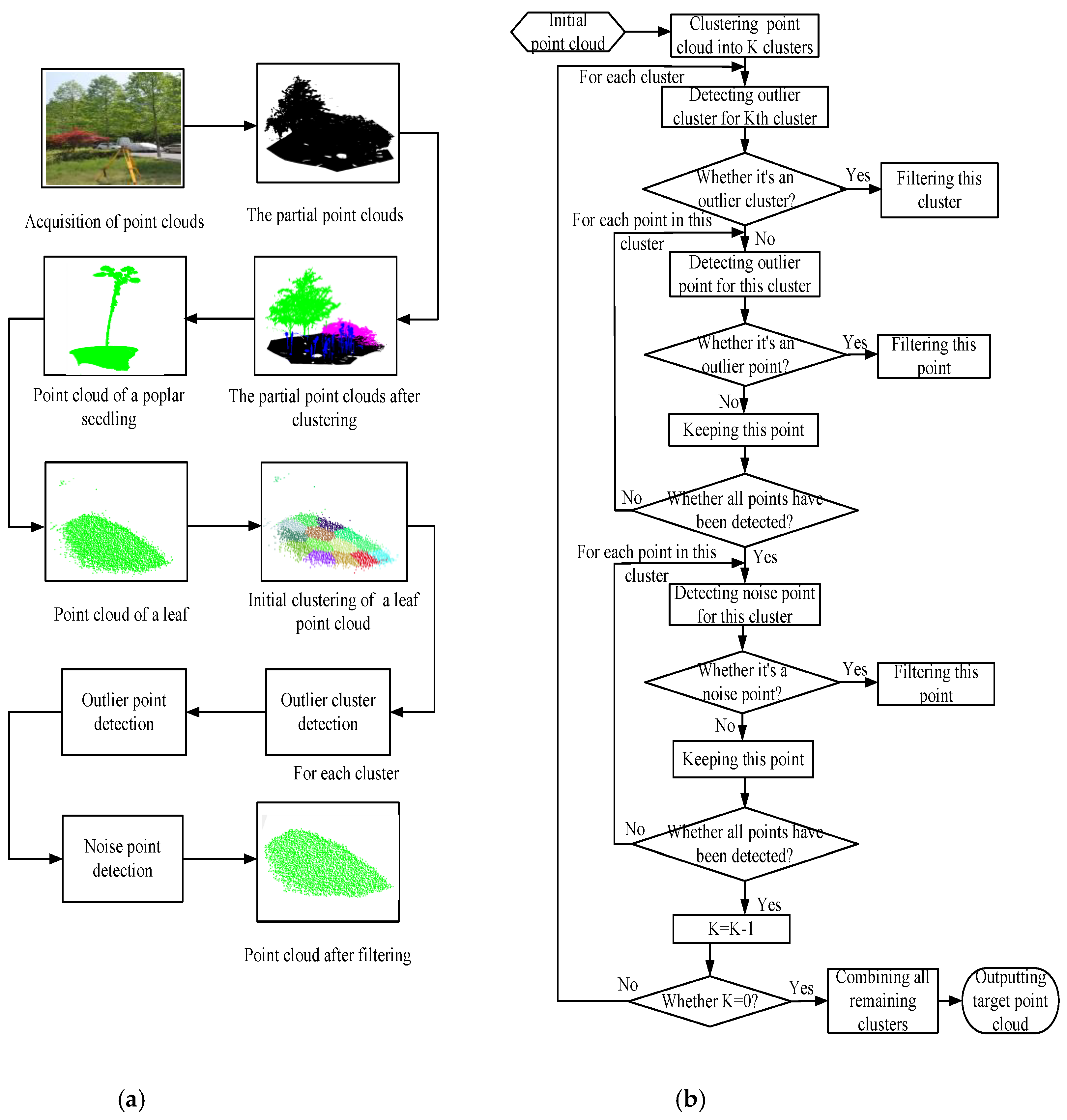
2.1. Data Collection by TLS

A terrestrial laser scanner (TLS, Leica C10) was used to obtain point cloud data. This scanner is a single-point-positioning scanner with high accuracy and precision. It can obtain massive point clouds efficiently and quickly without any intervention. The maximum scanning distance of the Leica C10 is 300 m and the scanning range is ${360}^{°}\times {270}^{°}$ (horizontal × vertical). While scanning, the TLS was placed successively on different sides 3m from the target tree. After scanning, each scan from the different angle was integrated into a single coordinate system by using a registration process to acquire full coverage scanning data from the objective trees. The experimental trees were selected on the campus of Nanjing Forestry University (32°08′N, 118°81′E) and included several species, such as poplar, sakura and Liriodendron chinensis.

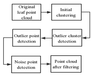
2.2. Framework of the Proposed Method

This section describes in detail the method we proposed for 3D point cloud filtering for leaves. Partial point clouds were manually segmented from the whole point clouds scanned by the Leica C10. The method in Reference [32] was employed to cluster the partial point clouds and extract well-isolated individual trees from groups. The point clouds of leaves were separated using the tree organ classification method proposed in Reference [8]. Taking a poplar leaf as an example, the whole process, from the acquisition of the point cloud to the point cloud after filtering, followed the sequential steps shown in Figure 1a.

The points that were to be filtered contained both outliers and noise, which had totally different definitions in this study. The exact definition of an outlier often depends on hidden assumptions regarding the data structure and the applied detection method [33]. Hawkins et al. [34] defined an outlier as an observation that deviates so much from other observations as to arise suspicion that it is generated by a different mechanism. Barnett et al. [35] indicated that an outlying observation or outlier, is one that appears to deviate markedly from other members of the sample in which it occurs. In this study, outliers were defined in a distance-based manner and divided into two categories: outlier clusters and outlier points. The manifold distance was used for distance measurement instead of the traditional Euclidean distance. Outlier clusters are more subject to masking and swamping effects, which are universal phenomena in outlier detection. Acuna et al. [36] provided an intuitive definition of these effects. If an outlier cluster is treated the same as a series of individual outlier points, these circumstances are more likely to occur. Hence, in this method, outlier cluster detection was the first step after the initial clustering. Subsequently, in each remaining cluster, outlier point detection and noise point detection were successively processed. At last, combining all remaining points and the point cloud after filtering was obtained. The detailed work program flow of the proposed method is shown in Figure 1b.

2.3. Adapted Truncation Method

The truncation method is a technique used to filter abnormal values in a data set. For a given data set $q_i$, $\left(i=1,2,\dots ,M\right)$, which is sorted in ascending order and $M$ is the total number of this data set. The quartiles of this data set divide it into four equal parts, each of which contains 25 percent of the data. The numbers at the first quorum and the third quorum are lower quartile $Q_1$ and upper quartile $Q_3$, respectively, which are expressed as follows:

$$Q_1=\{\begin{array}{cc}{q}_{\left(\left[0.25M\right]+1\right)}& 0.25M\mathrm{is}\mathrm{not}\mathrm{an}\mathrm{integer}\\ \frac{q_{\left(0.25M\right)}+q_{\left(0.25M+1\right)}}{2}& 0.25M\mathrm{is}\mathrm{an}\mathrm{integer}\end{array}$$

(1)

and

$$Q_3=\{\begin{array}{cc}{q}_{\left(\left[0.75M\right]+1\right)}& 0.75M\mathrm{is}\mathrm{not}\mathrm{an}\mathrm{integer}\\ \frac{q_{\left(0.75M\right)}+q_{\left(0.75M+1\right)}}{2}& 0.75M\mathrm{is}\mathrm{an}\mathrm{integer}\end{array}$$

(2)

The specific procedures of the truncation method to filter abnormal values in the data set are as follows:

First, calculating $Q_1$ and $Q_3$ using Equation (1) and Equation (2);

Second, calculating the interquartile range $R_{iq}$, which can be formulated by

$$R_{iq}=Q_3-Q_1$$

(3)

Third, calculating the lower truncation $T_L$ and upper truncation $T_H$ according to the following formula:

$$T_L=Q_1-\mu \cdot R_{iq}$$

(4)

and

$$T_H=Q_3+\mu \cdot R_{iq}$$

(5)

while $\mu$ denotes the threshold value of the truncation method. $q_i<T_L$ and $q_i>T_H$ are defined as the abnormal values of this data set.

In the universal truncation method, the threshold value $\mu$ usually equals 1.5. Although using quartiles as numerical characteristics makes the method robust, it is more suitable for data with a regular distribution, such as a normal distribution. Most abnormal values would be omitted by a smaller $T_L$ and larger $T_H$. Hence, it was inappropriate for our point cloud data. A more suitable threshold value is given in this study.

2.4. Outlier Detection and Filtering in Manifold Space

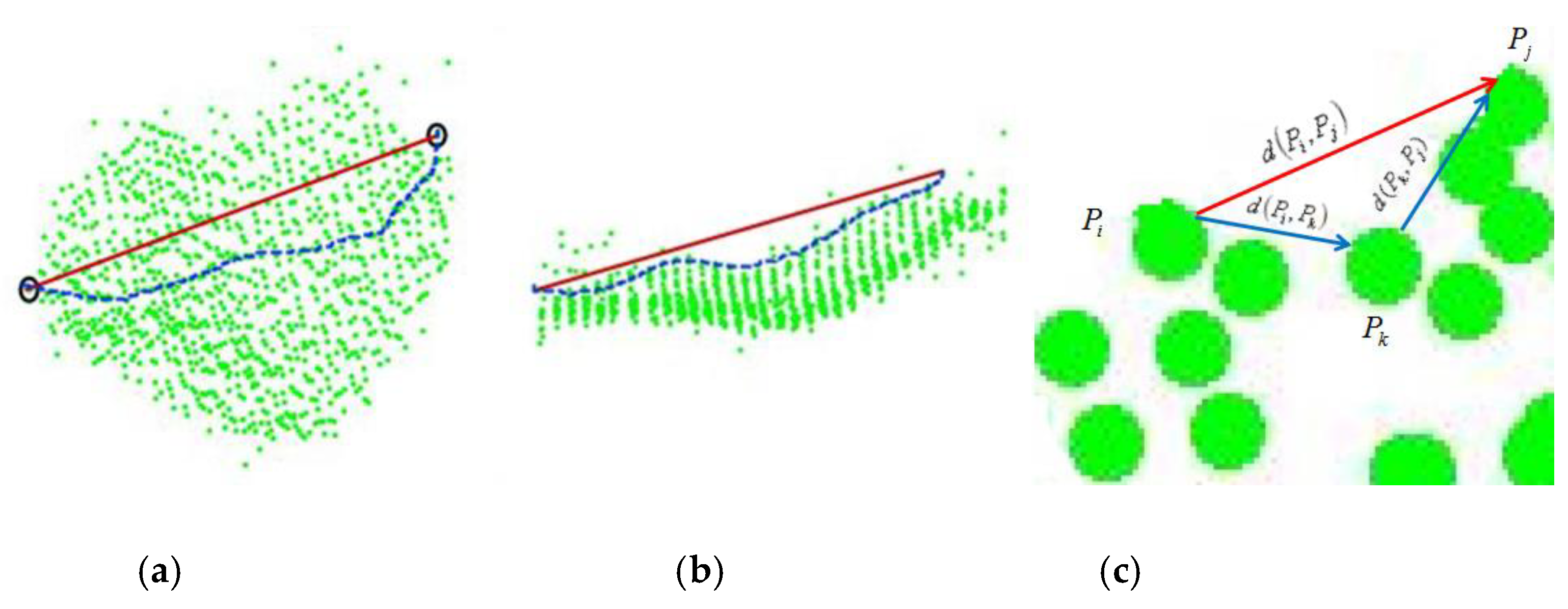
2.4.1. Measuring Manifold Distance

Points on adjacent positions have high similarities. However, the Euclidean distance can measure only local congruence instead of that of the whole point cloud. Figure 2a presents the two connection modes of two points in a point cloud from the front view and Figure 2b shows the horizontal view. Clearly, the Euclidean distance in the red line between two points cannot reflect the whole manifold similarities well, while the connection mode in blue, which we call the geodesic curve, better reflects the similarities between these two points. A geodesic curve in differential geometry is defined as follows: for any curve on a surface, the geodesic curvature of each point on it is zero. All points on the geodesic curve are on the surface and the distance between two points is shorter than any other paths between these two points. This distance, which we call the shortest path, more accurately reflects the similarities between two points on a surface. The shortest path problem is broad but the variable weight in this study refers to the distance between two points.

For a sample point cloud $P$, $P_i\in P$ and $P_j\in P$, $\left(i,j=1,2,\dots ,N\right)$, $N$ is the number of points and two methods can be used to find the shortest path between $P_i$ and $P_j$. One method is to go directly from $P_i$ to $P_j$; the other is to go to $P_j$ through point $P_k\in P$, $\left(k=1,2,\dots ,N\right)$, as depicted in Figure 2c, which is the local enlarged point cloud of Figure 2a,b. Defining $d\left(P_i,P_j\right)$ and $d^{\prime }\left(P_i,P_j\right)$ as the distance and the shortest distance between $P_i$ and $P_j$, we obtain

$$d^{\prime }(p_i,p_j)=\{\begin{array}{cc}d(P_i,P_j)& d(P_i,P_j)<d(P_i,P_k)+d(P_k,P_j)\\ d(P_i,P_k)+d(P_k,P_j)& d(P_i,P_j)>d(P_i,P_k)+d(P_k,P_j)\end{array}$$

(6)

Common solutions of the shortest path problem include the Floyd, Dijkstra and Bellman-Ford algorithms [37]. Among these algorithms, the traditional Floyd algorithm is globally optimal and the main program is simple, easy to implement. Therefore, the Floyd algorithm was used in this study.

Constructing the adjacency matrix $D_{N\times N}$ and iterating $D_{N\times N}$ to approximate the manifold distance by the traditional Euclidean distance are the key steps in the Floyd algorithm. Using the two methods mentioned previously in the lemma, the main procedures are as follows:

First, for points $P_i\left(x_i,y_i,z_i\right)$ and $P_j\left(x_j,y_j,z_j\right)$, the traditional Euclidean distance is defined as

$$d\left(P_i,P_j\right)=\sqrt{{\left(x_i-x_j\right)}^2+{\left(y_i-y_j\right)}^2+{\left(z_i-z_j\right)}^2}$$

(7)

and for any positive integer $k$, ${\mathsf{\phi }}_i=\left\{P_{im}\right\}$, $\left(m=1,2,\dots ,k\right)$ can be determined, where $P_{im}$ represents the $k$ nearest neighbor of point $P_i$.

Second, initializing the adjacency matrix $D_{N\times N}$, $D\left(i,j\right)$ is as follows:

$$D\left(i,j\right)=\{\begin{array}{cc}d(P_i,P_j)& P_j\in {\mathsf{\phi }}_i\\ +\infty & P_j\notin {\mathsf{\phi }}_i\end{array}$$

(8)

Third, the distance matrix $D_{N\times N}$ is iterated continuously using Equation (6) and (8) while traversing all points in the data set. Until the iteration terminates, each element $D\left(i,j\right)$ is represented as the manifold distance between points $P_i$ and $P_j$.

However, the Floyd algorithm, as discussed above, essentially proceeds through a triple loop. Excessive iteration leads to computational complexity and requires an extremely large amount of storage, especially for a large number of nodes. Unfortunately, the point cloud scanned by TLS are usually numerous and in high density. Two improvements of the Floyd algorithm were proposed by Wei [38]. The first improvement is the construction of an iterative matrix in which all nodes are initially compared; nodes that are not related to the results are removed to reduce the frequency of iteration when searching for the next node. Second, a serial number matrix is constructed to record the case of inserting a node in the process of iteration. Aini et al. [39] named another contribution: the rectangular algorithm. This algorithm benefits from a rectangle graphical approach, requires less computational effort and is easier to implement than the Floyd algorithm. However, both of these methods focus on the iteration process itself. Our proposed method deals with the data size directly. The initial clustering is processed at the beginning and under this condition, the method can proceed with the Floyd algorithm for only one cluster at a time. Without removing any points or constructing any new matrices, the computational time is reduced.

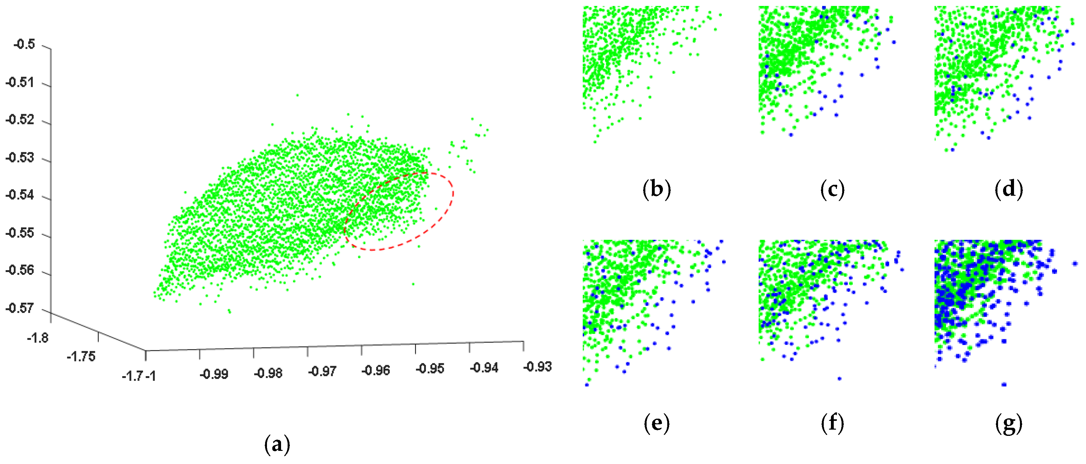
2.4.2. Filtering Outlier Clusters

As illustrated, initial clustering is the preprocessing step in this method. The K-means clustering, which is simple and easy to implement, was used to divide the original point cloud $P$ into $K$ clusters, which denoted by $R_l$, $\left(l=1,2,\dots ,K\right)$. $K$ is an integer by rounding up $N/100$ and $N$ represents the number of points.

To measure how far cluster $R_l$ is from the other $K-1$ clusters, which denoted by $d_C^{\prime }\left(l\right)$, the mathematical models are as follows:

$$C_l=\frac{1}{N_l}{\displaystyle \sum _{l_i=1}^{N_l}{P}_{l_i}(x_{l_i},y_{l_i},z_{l_i})}$$

(9)

and

$$d_C^{\prime }\left(l\right)={\displaystyle \sum _{\begin{array}{c}{l}^{\prime }=1\\ l\ne l^{\prime }\end{array}}^K{d}_C\left(l,l^{\prime }\right)}$$

(10)

where $C_l$ is the center of $R_l$, $P_{l_i}$, $\left(i=1,2,\dots ,N_l\right)$ are the points in cluster $R_l$, $N_l$ represents the number of points and $d_c\left(l,l^{\prime }\right)$ represents the manifold distance between clusters $C_l$ and $C_{l^{\prime }}$. Using the truncation method with the newly defined threshold value ${\mu }^{\prime }$ to calculate the upper truncation $T_{H_1}$ of data set $d_C^{\prime }$ and a cluster is defined as an outlier cluster when its $d_C^{\prime }\left(l\right)$ is bigger than $T_{H_1}$.

The detailed procedures are given as follows:

Input: Point cloud $P$

Divide the original point cloud data into $K$ clusters Calculate $C_l$ of $R_l$ using Equation (9) Calculate $d_c\left(l,l^{\prime }\right)$ using the method in 2.4.1 Calculate $d_C^{\prime }\left(l\right)$ using Equation (10) Calculate $T_{H_1}$ of $d_C^{\prime }$ using Equation (5) and ${\mu }^{\prime }$ For $l=1:K$   if $d_C^{\prime }(l)>T_{H_1}$   Define $R_l$ as an outlier cluster and remove $R_l$   end if end for

Output: New clusters without outlier clusters: $R_l^{\prime }$, $\left(l=1,2,\dots ,K^{\prime }\right)$

2.4.3. Filtering Outlier Points

After filtering the outlier clusters, new clusters without outlier clusters $R_l^{\prime }$, $\left(l=1,2,\dots ,K^{\prime }\right)$ and points $P_{l_i}$, $\left(i=1,2,\dots N_l\right)$ in $R_l^{\prime }$ are obtained, where $K^{\prime }$ represents the number of remaining new clusters. The manifold distance between point $P_{l_i}$ and $P_{l_j}$ in cluster $R_l^{\prime }$, denoted by $d_p\left(l_i,l_j\right)$, can be used to obtain $k$ nearest points of $P_{l_i}$, which is expressed as ${\mathsf{\phi }}_{l_i}=\left\{P_{l_{im}}\right\}$, $\left(m=1,2,\dots ,k\right)$.

For each cluster, to measure how far the point $P_{l_i}$ is from the other points in this cluster, which denoted by $d_p^{\prime }\left(l_i\right)$, the mathematical model is:

$$d_p^{\prime }\left(l_i\right)={\displaystyle \sum _{m=1}^k{d}_p\left(l_i,l_{im}\right)}$$

(11)

Calculating the upper truncation $T_{H_2}$ of data set $d_p^{\prime }\left(l\right)$ and a point is defined as an outlier point in this cluster when its $d_p^{\prime }\left(l_i\right)$ is bigger than $T_{H_2}$.

The detailed procedures are given as follows:

Input: $R_l^{\prime }$, $\left(l=1,2,\dots ,K^{\prime }\right)$, $P_{l_i}\in R_l^{\prime }$, $\left(i=1,2,\dots ,N_l\right)$

for $l=1:K^{\prime }$   Calculate $d_p\left(l_i,l_j\right)$ using the method in 2.4.1   for $i=1:N_l$    Find ${\mathsf{\phi }}_{l_i}=\left\{P_{l_{im}}\right\}$, $\left(m=1,2,\dots ,k\right)$ of $P_{l_i}$ and $k=10$    Calculate $d_p^{\prime }\left(l_i\right)$ using Equation (11)   end for   Calculate the upper truncation $T_{H_2}$ of $d_p^{\prime }\left(l\right)$ using Equation (5) and ${\mu }^{\prime }$   for $i=1:N_l$    if $d_p^{\prime }\left(l_i\right)>T_{H_2}$      Define $P_{l_i}$ as the outlier point and remove $P_{l_i}$    end if   end for end for

Output: Clusters $R_l^{\prime }$ without outlier points: ${P_{l_i}}^{\prime }\in R_l^{\prime }$, $\left(i=1,2,\dots ,N_l^{\prime }\right)$

2.5. Noise Detection and Filtering Based on the Normal Feature of Local Surfaces

2.5.1. Local Surface Fitting and Normal Estimation

PCA is a dimensional reduction method used in feature extraction, especially for surface normal estimations. For a given data point $P_i$ and its $k$ nearest neighbor set ${\mathsf{\phi }}_i=\left\{P_{im}\right\}$, the covariance matrix $C_{3\times 3}$ of this local neighborhood is defined as follows:

$$C_{3\times 3}=\frac{1}{k}{{\displaystyle \sum _{m=1}^k\left(P_{im}-{\overline{P}}_i\right)}}^T\left(P_{im}-{\overline{P}}_i\right)$$

(12)

where ${\overline{P}}_i$ is the mean of ${\mathsf{\phi }}_i=\left\{P_{im}\right\}$ and can be calculated by the following formula:

$${\overline{P}}_i=\frac{1}{k}{\displaystyle \sum _{m=1}^k{P}_{im}}$$

(13)

Using singular value decomposition (SVD), $C_{3\times 3}$ can be decomposed into three principal components $v_1,v_2,v_3$, which are the three eigenvectors corresponding to the eigenvalues ${\lambda }_1,{\lambda }_2,{\lambda }_3$, respectively, sorted in descending order. The third principal component $v_3$ corresponds to the direction in which the projected observations have the smallest variance, which means that eigenvector $v_3$ approximates the normal direction of this local neighborhood.

However, many previous studies have pointed out that PCA is sensitive to outliers and fails to reliably fit planar surfaces in the presence of outliers [40]. Hence, many methods that can make PCA results robust have been proposed. Hubert et al. [41] combined robust covariance estimation with Projection Pursuit and proposed RPCA. They claimed that their method yielded accurate estimates for outlier-free datasets and more robust estimates for outlier-contaminated data and had the further advantage of outlier detection [32]. Rousseeuw et al. [42] developed fast-MCD in 1999 and Nurunnabi et al. [43] used fast-MCD-based RPCA to fit a planar surface. However, most of the above methods have yielded limited improvements in the definition of the distance weight. Traditional PCA compares Euclidean distances of potential target points to find the local neighborhood of one point. It provides less robust local neighborhood relationships for our point cloud data, which is crucial for deciding which points should contribute to the normal estimations. To increase the accuracy of the results, the manifold distance in $D_{N\times N}$ is used in this study to construct the local neighborhood and calculate the normal estimation of each point.

2.5.2. Filtering Noise Points

After filtering outliers, remaining new clusters, $R_l^{\prime }$, $\left(l=1,2,\dots ,K^{\prime }\right)$ and points ${P_{l_i}}^{\prime }$, $\left(i=1,2,\dots ,{N^{\prime }}_l\right)$ in $R_l^{\prime }$, were obtained, while $N_l^{\prime }$ represents the new number of points in $R_l^{\prime }$. For each cluster, using the manifold distance to construct $k$ nearest neighbor set ${{\mathsf{\phi }}_{l_i}}^{\prime }=\left\{{P_{l_{im}}}^{\prime }\right\}$, $\left(m=1,2,\dots ,k\right)$ of each point ${P_{l_i}}^{\prime }\left(x_{l_i},y_{l_i},z_{l_i}\right)$ and the angle between this point and its normal direction $v_{3_{l_i}}(v_{x_{l_i}},v_{y_{l_i}},v_{z_{l_i}})$ was used to decide whether this point is the noise point in this cluster, which can be described as follows:

$$\theta \left(l_i\right)=\frac{\left(x_{l_i}\cdot v_{x_{l_i}}+y_{l_i}\cdot v_{y_{l_i}}+z_{l_i}\cdot v_{z_{l_i}}\right)}{{\left(x_{l_i}{}^2+y_{l_i}{}^2+z_{l_i}{}^2\right)}^{1/2}\cdot {\left(v_{x_{l_i}}{}^2+v_{y_{l_i}}{}^2+v_{z_{l_i}}{}^2\right)}^{1/2}}$$

(14)

Calculating the lower truncation $T_{L_3}$ and upper truncation $T_{H_3}$ of the $\theta \left(l\right)$ and points, angles of which are between these two bounds, will be retained. Otherwise, they are removed as noise points.

The detailed procedures are given as follows:

Input: $R_l^{\prime }$, $\left(l=1,2,\dots ,K^{\prime }\right)$, ${P_{l_i}}^{\prime }\in R_l^{\prime }$, $\left(i=1,2,\dots ,N_l^{\prime }\right)$

for $l=1:K^{\prime }$   for $i=1:{N^{\prime }}_l$    Find ${{\mathsf{\phi }}_{l_i}}^{\prime }=\left\{{P_{l_{im}}}^{\prime }\right\}$, $\left(m=1,2,\dots ,k\right)$ of ${P_{l_i}}^{\prime }$ and $k=10$    Calculate $v_{3_{l_i}}$ of point ${P_{l_i}}^{\prime }$ using Equation (12), Equation (13) and SVD    Calculate $\theta \left(l_i\right)$ using Equation (14)   end for    Calculate $T_{L_3}$ and $T_{H_3}$ of $\theta \left(l\right)$    for $i=1:N_l^{\prime }$    if $\theta (l_i)<T_{L_3}$ or $\theta (l_i)>T_{H_3}$     Define ${P_{l_i}}^{\prime }$ as a noise point and remove ${P_{l_i}}^{\prime }$    end if   end for end for

Output: Cluster $R_l^{\prime }$ without outlier and noise points, $P_{l_i}^{″}\in R_l^{\prime }$, $\left(i=1,2,\dots ,N_l^{″}\right)$

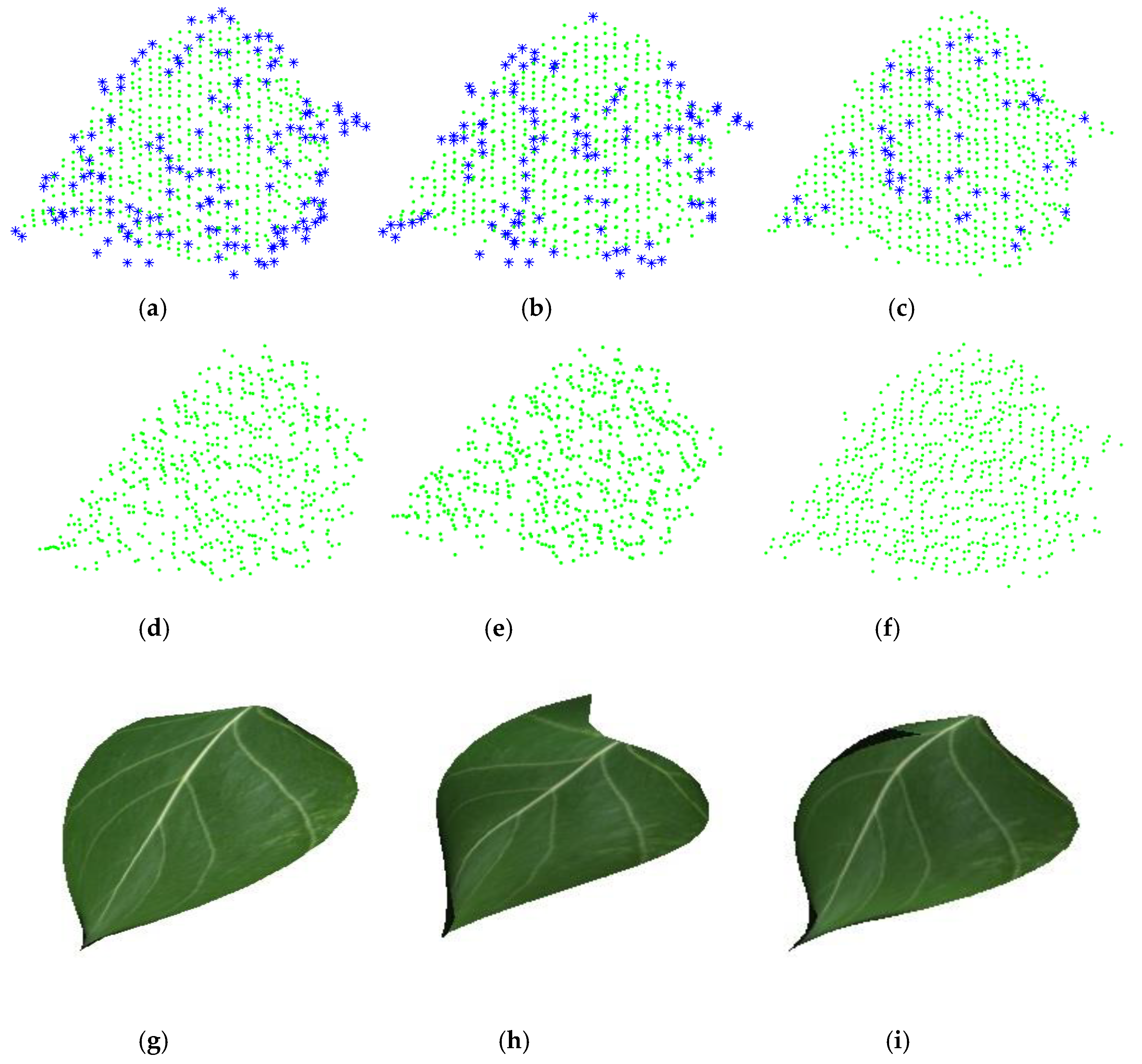
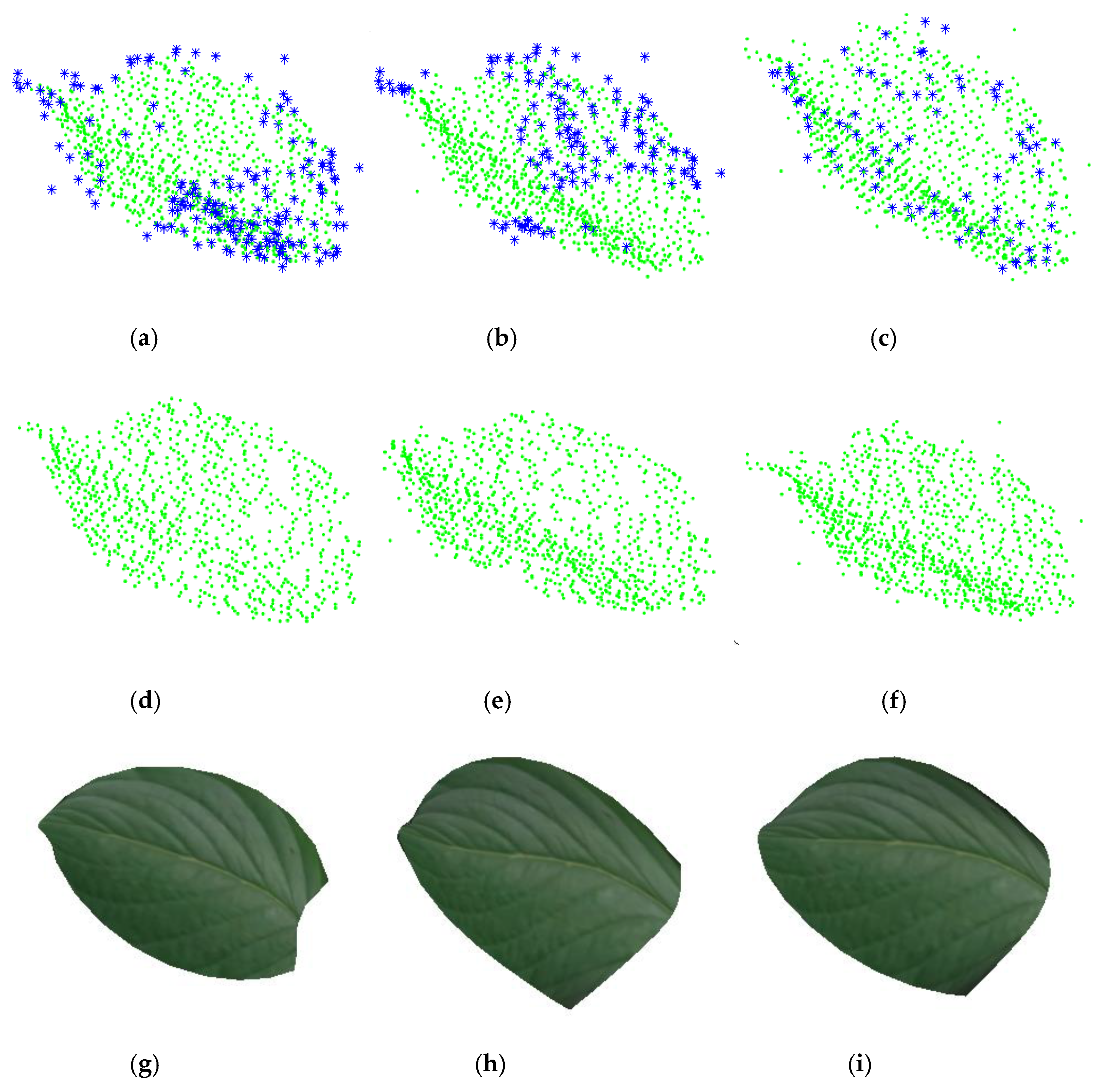
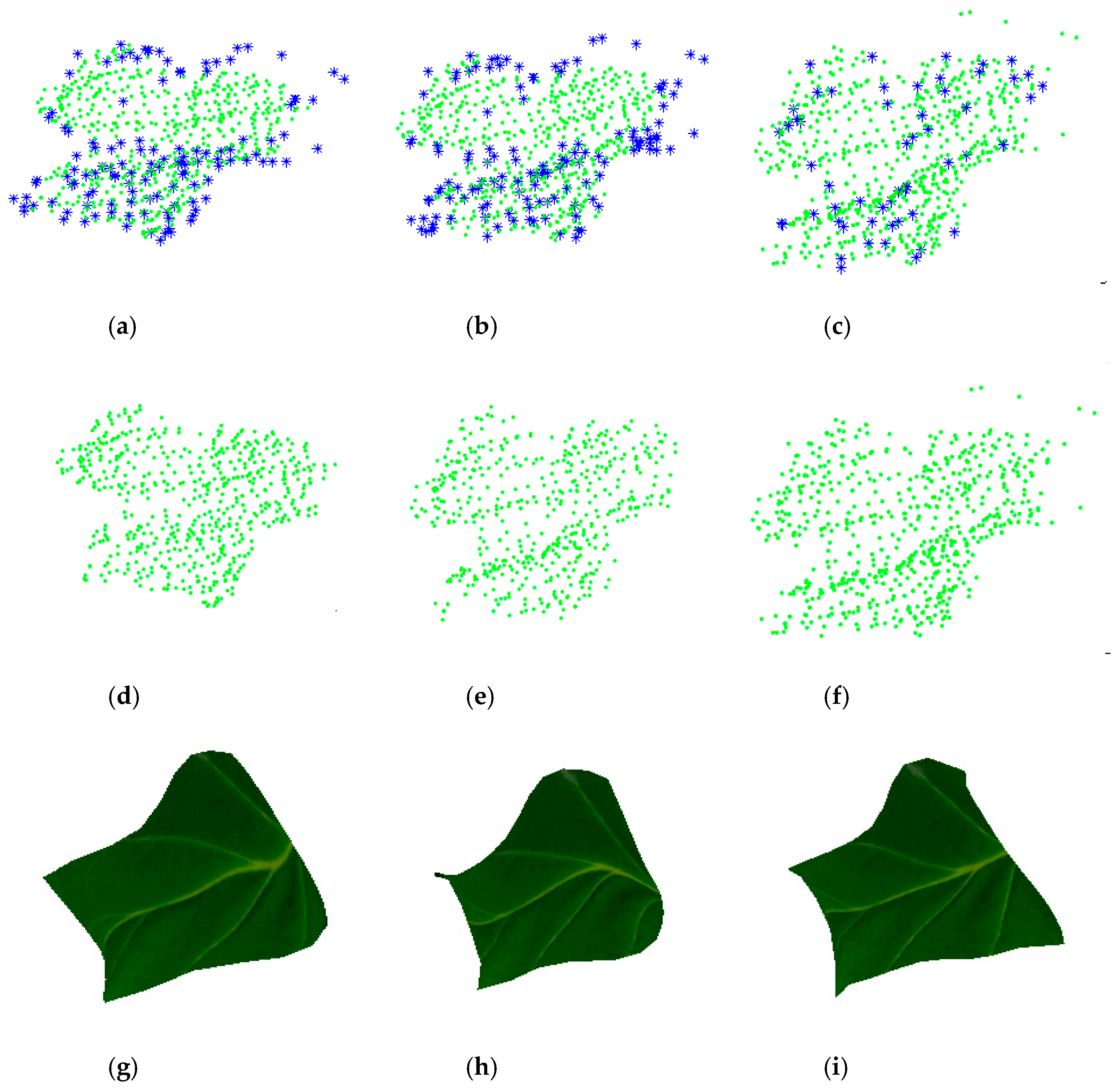
3. Experiments and Results Analysis

Numerous comparison analyses were performed to evaluate the effectiveness and practicability of the proposed method. Leaves of trees with different heights and diameters at breast height (DBH) were collected as analysis samples, as shown in

Table 1. Summary of sample tree and leaf parameters.

	Minimum	Maximum	Mean	Standard Deviation
Tree height (m)	0.71	10.8	6.2	3.6
Tree DBH (cm)	1.2	20.6	12.7	5.1
Leaf point Number	189	752	423	112
Leaf length (cm)	3.4	12.4	7.1	1.9
Leaf width (cm)	2.7	10.5	6.2	1.8

. In Section 3.1, the effects of the different threshold values of the truncation method on the recognition rates are compared intuitively. In Section 3.2, the proposed method is compared with two other methods to evaluate the filtering performance of the proposed method. 3D reconstruction and visualization results are also presented in this section. In Section 3.3, analyses of leaf area measurement are given to further verify the applicability of the proposed method.

3.1. Effects of the Threshold Value $\mu$ on Recognition Rates

Different threshold value $\mu$ resulted in totally different filtering performance for the leaf point cloud. To find a suitable threshold value for our point cloud, this study tested five different values for each leaf sample, with $0.3$ as the interval. Figure 3 gives a poplar leaf sample.

The points in blue are the outliers and noise detected by the truncation method. Clearly, when $\mu =1.5$, the recognition rate is very low. In addition, compared with Figure 3d,e, Figure 3f reveals a better filtering performance. However, when $\mu =0.3$ in Figure 3g, the point cloud is oversmoothed. The results demonstrated that the threshold value $\mu =0.6$ was suitable for the leaf point cloud.

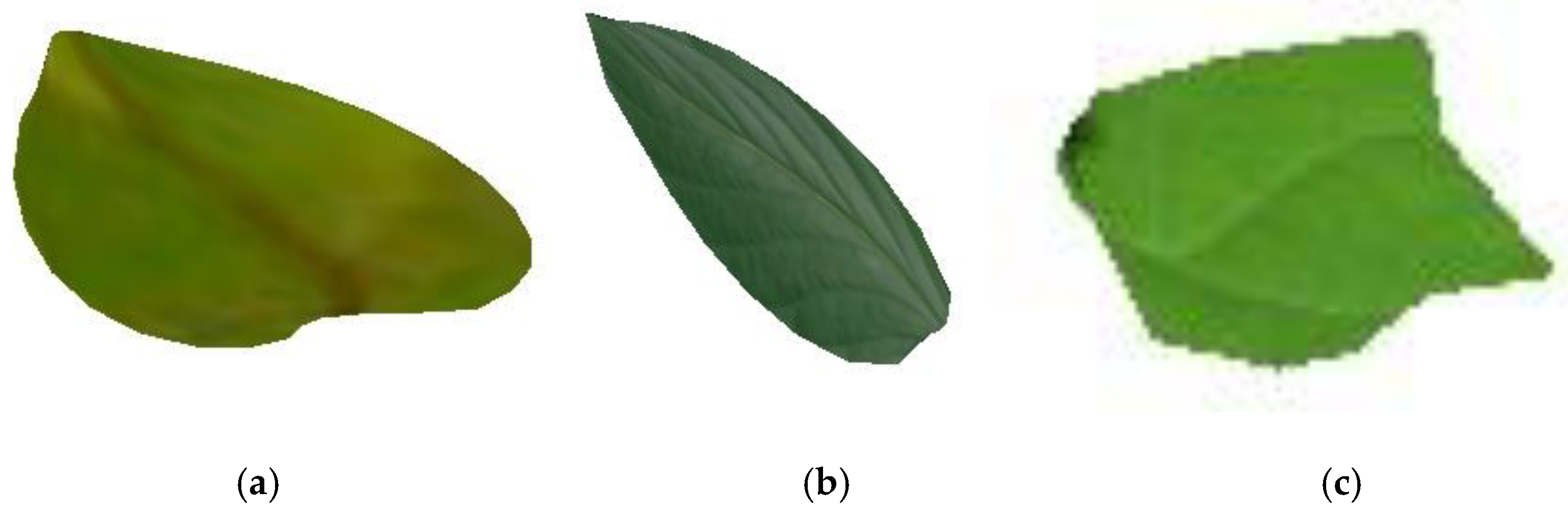
3.2. Filtering Performance Evaluation Based on 3D Reconstruction

The method we proposed has two main innovations: filtering outlier clusters, outlier points and noise points separately and using manifold distance as a metric. To highlight the advantages of these two innovations, the comparison analyses were carried out with other two methods: using the Euclidean distance method and classical PCA method. The Euclidean distance method uses the same procedures as the method we proposed excluding the use of manifold distance and classical PCA is a standard method that neither filters outliers and noise separately nor uses manifold distance.

Leaves of different species and levels were chosen from the collected samples to conduct a comprehensive assessment. 3D reconstructions of leaves were obtained by the nonuniform rational B-spline (NURBS) method, which has become a widely utilized approach for surface reconstruction in recent years [37,44]. The presence of outliers and noise would mislead the choices of control points in NURBS, which indirectly influence the fitting performance. Moreover, 3D visualizations of the samples were constructed using VC++ 2015 and OpenGL.

To demonstrate the performance of filtering using different methods, mature leaves were taken as examples. Figure 4 shows the experimental results for a mature poplar leaf. The blue points in Figure 4a–c, which represent outliers and noise found by the filtering methods, reveal that the proposed method generally had better performance in terms of both quality and quantity in filtering, resulting in better reconstruction of the point cloud. The proposed method and method using the Euclidean distance method, all treated outlier clusters and points separately, thereby avoiding masking and swamping effects to some extent, whereas the classical PCA, as shown in Figure 4c,f, had the worst filtering results. Comparison results fully explains why it is necessary to filter outlier clusters and points separately. In addition, the point cloud after filtering in Figure 4d is closer to the shape of the real leaf than that in Figure 4e,f. Hence, the reconstruction and visualization in Figure 4g outperformed that in Figure 4h,i.

For the mature sakura leaf point cloud, as shown in Figure 5a,b, the method we proposed and the Euclidean distance method yielded almost completely different filtering results because the leaf surfaces of sakura are usually curved. Consequently, using the manifold distance or not has great effects on the sakura leaf point cloud. The results in Figure 5c,f reveal that classical PCA was still not good for filtering sakura leaf point cloud. Moreover, outliers and noise, which were omitted in filtering, directly caused the distortion of the 3D reconstruction in Figure 5h,i.

Figure 6 gives the experimental results for a mature Liriodendron chinense leaf. The Liriodendron chinense leaf surface has many corners and edges. Hence, better filtering result was required for the its reconstruction and visualization. As shown in Figure 6e, the method using Euclidean distance omitted four single outliers in the lower left corner of the point cloud and the reconstruction of this leaf is out of shape in this position. Similarly, classical PCA could not handle points in the corners well and thus the reconstruction result in Figure 6i has sharper corners.

In addition to mature leaves, tender leaves can also reflect the growth status of trees. Hence, 3D reconstruction results of tender leaves from the three species above were also given in Figure 7. The leaf areas of tender leaves are usually small. Although they have fewer points than mature leaves, the reconstruction and visualization of them are still real after filtering with the proposed method. It proves that the method we proposed can be applied to different leaves of different species and levels.

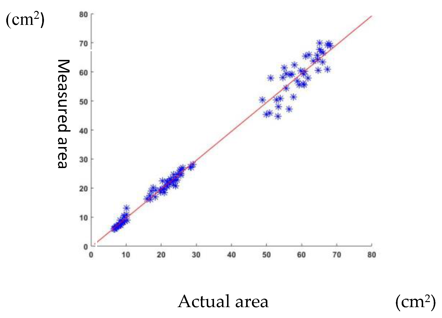
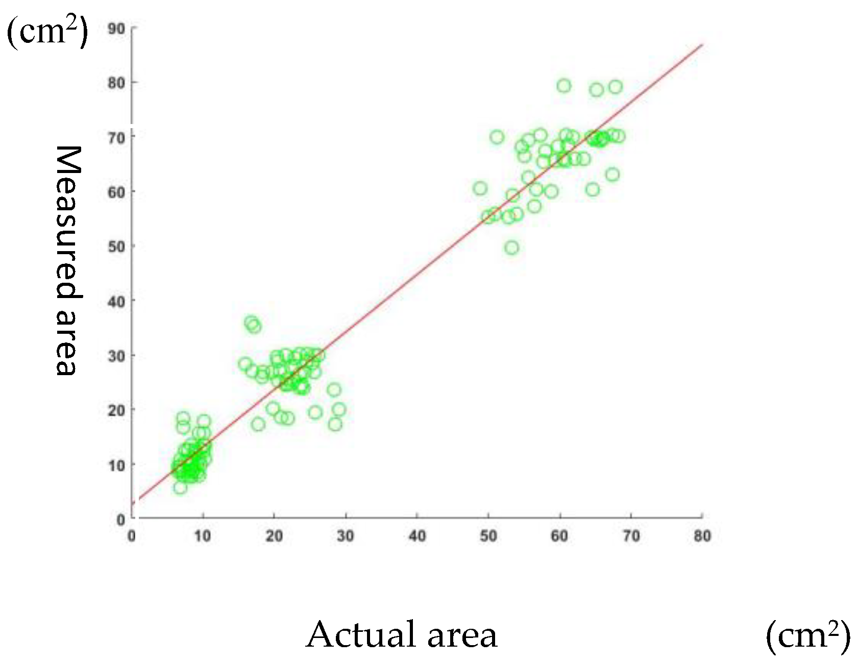
3.3. Leaf Area Measurement

The 3D reconstruction and visualization of the point cloud can be used to estimate many complex leaf traits. Leaf area is one of these traits and the application of the partial mesh area method based on the NURBS fitting surface can be used to calculate the leaf area [45]. To further validate the performance of the proposed filtering method, leaf areas of samples of different sizes were calculated and 120 of them, which areas ranged from 5 to 80 cm², were randomly chosen in analyses of leaf area measurement. Two comparisons were conducted: one was the comparison of the leaf area measurements after filtering using the proposed method and the actual area, as described in Figure 8 and the other one was the comparison of the leaf area measurements after filtering using classical PCA and the actual area, as described in Figure 9. The actual leaf area was obtained by manual measurement using an LI-3000C area meter. As shown in Figure 8, the RMSE of leaf area regression is 2.49 cm² and R-square is 0.98. However, the RMSE is 5.02 cm² and R-square is 0.95 in Figure 9. The measurement results from the 3D reconstruction of the point clouds after filtering with the proposed method were closer to the actual area values, which also indicated that the proposed filtering method can improve the performance of leaf area measurement.

Moreover, another comparison analyses using 120 leaf samples were conducted to further analyze the impacts that the filtering method had on leaves with different areas. These 120 leaves were classified as small leaves (SFs), with areas of 5 cm²–15 cm²; medium leaves (MFs), with areas of 16 cm²–40 cm²; and large leaves (LFs), with areas of 41 cm²–80 cm². The mean absolute error (MAE) and mean absolute error percent (MAE%) of the samples filtered using the proposed method and classical PCA were separately calculated in analyses as follows:

$$\mathrm{MAE}={\displaystyle \sum _{i=1}^n\left|\frac{A_i-{\widehat{A}}_i}{n}\right|}$$

(15)

and

$$\mathrm{MAE}\%=\frac{1}{n}{\displaystyle \sum _{i=1}^n\left|\frac{A_i-{\widehat{A}}_i}{A_i}\right|}\times 100\%$$

(16)

where $A_i$ and ${\widehat{A}}_i$ are the actual leaf area and the measured leaf area and $n$ is the number of leaf samples. For each type of sample, $n=40$.

Table 2. Comparison of the MAE and MAE% values for samples filtered with the proposed method and classical PCA.

	Filtering Using The Proposed Method			Filtering Using Classical PCA
Leaf Size	SF	MF	LF	SF	MF	LF
MAE (cm2)	0.92	1.05	3.39	2.76	5.61	6.83
MAE%	10.63	4.83	3.8	33.68	27.05	11.79

gave the comparison results of the MAE and MAE% values for samples filtered by the proposed method and classical PCA. Clearly, the MAE and MAE% of the samples filtered using the proposed method are less than those filtered by classical PCA. This difference was more obvious when the area was smaller, especially for SFs.

4. Discussion

4.1. Comparison with Existing Methods

In this paper, a new method for 3D leaf point cloud filtering was proposed. Above all, as discussed before, the Floyd algorithm suffers from high computational complexity, especially for large-scale point cloud data. Although [38] and [39] improved the Floyd algorithm, they did not deal with the data size directly. In this paper, the original point cloud data were initially clustered and under this circumstance, the Floyd algorithm proceeded with only one cluster with a fixed number of points at one time. In addition, a new filtering strategy was also used in the method. Previously, Sridhar et al. [46] proposed a formulation for outliers based on the distance of a point from its Kth nearest neighbors. They ranked each point on the basis of its distance to its Kth nearest neighbor and classified the top points in this ranking as outliers. Breunig et al. [47] used the local outlier factor (LOF) to measure the outlier degree of an object. Although these methods are practical for finding local outliers, they do not filter outlier clusters and outlier points separately. In this study, after the initial clustering was performed, outlier clusters were filtered and then outlier points were filtered. This strategy weakens the masking and swamping effects of outlier clusters and shows better filtering performance. Moreover, in this study, a manifold distance-based PCA method was applied for noise detection. PCA is a neighborhood-based filtering technique. This technique determines the filtered position of a point using similarity measures between a point and its neighborhood, which has a strong influence on the efficiency and effectiveness of the filtering approach [48]. The similarity can be defined by the positions of points, normals or regions [49]. Many previous PCA-based methods constructed neighborhoods using the traditional Euclidean distance. However, using the manifold distance to construct a local plane surface and determine which points should contribute to the normal estimations helps achieve more robust features and better filtering performance.

4.2. Recommendations

The method we proposed uses an adaptive threshold value in the truncation method to filter abnormal values. Figure 3 shows the filtering performance of this threshold value and the result was satisfactory. In fact, the filtering accuracy of the truncation method for point cloud data depends strongly on the properties of the point cloud data, such as scale and density, rather than the threshold value itself. Although the experimental results proved that the threshold value used in this method was appropriate for leaf point cloud data, for other specific point cloud data, specific analyses and comparisons should be performed to choose the suitable threshold value in the truncation method to ensure the filtering effect.

5. Conclusions

In this study, a 3D point cloud filtering method for leaves based on manifold distance and normal estimation was proposed and point cloud data were collected using a Leica C10 terrestrial laser scanner. First, the original point cloud was initialized into several clusters and the truncation method with the newly defined threshold value was used to filter outlier clusters. Second, for each new cluster, the outlier points were filtered using the same truncation method and noise points were then filltered by normal estimations and included angles. The truncation method was used again to filter points with singular angles. After traversing all clusters, the filtering process was complete. Three analyses were conducted in this study: an analysis of a suitable threshold value in the truncation method, a comparison of the filtering performance between the proposed method and two other methods and an evaluation of the leaf area measurement. The first analysis proved that the truncation method with the new threshold value was suitable for point cloud data. The second analysis indicated that the proposed method had better filtering performance in terms of both quality and quantity than the method using Euclidean distance and classical PCA. The last analysis demonstrated that the area measurement results for leaves after filtering using the proposed method were closer to the actual leaf areas. Considering these results, the proposed method can be deemed as an improvement of 3D point cloud filtering method for leaves. From a practical perspective, the proposed method can be further used for 3D reconstruction and leaf trait measurement.

References

1. Giuliani, R.; Magnanini, E.; Nerozzi, F.; Muzzi, E.; Sinoquet, H. Canopy probabilistic reconstruction inferred from monte carlo point-intercept leaf sampling. Agric. For. Meteorol. 2005, 128, 17–32. [Google Scholar] [CrossRef]
2. Chaivivatrakul, S.; Tang, L.; Dailey, M.N.; Nakarmi, A.D. Automatic morphological trait characterization for corn plants via 3D holographic reconstruction. Comput. Electron. Agric. 2014, 109, 109–123. [Google Scholar] [CrossRef]
3. Zhu, X.; Zhu, M.; Ren, H. Method of plant leaf recognition based on improved deep convolutional neural network. Cogn. Syst. Res. 2018, 52, 223–233. [Google Scholar] [CrossRef]
4. Richter, R.; Reu, B.; Wirth, C.; Doktor, D.; Vohland, M. The use of airborne hyperspectral data for tree species classification in a species-rich Central European forest area. Int. J. Appl. Earth Obs. Geoinf. 2016, 52, 464–474. [Google Scholar] [CrossRef]
5. Oveland, I.; Hauglin, M.; Gobakken, T.; Næsset, E.; Maalen-Johansen, I. Automatic estimation of tree position and stem diameter using a moving terrestrial laser scanner. Remote Sens. 2017, 9, 350. [Google Scholar] [CrossRef]
6. Liu, C.; Xing, Y.; Duanmu, J.; Tian, X. Evaluating different methods for estimating diameter at breast height from terrestrial laser scanning. Remote Sens. 2018, 10, 513. [Google Scholar] [CrossRef]
7. Saremi, H.; Kumar, L.; Stone, C.; Melville, G.; Turner, R. Sub-compartment variation in tree height, stem diameter and stocking in a pinus radiata D. don plantation examined using airborne LiDAR data. Remote Sens. 2014, 6, 7592–7609. [Google Scholar] [CrossRef]
8. Yun, T. A novel approach for retrieving tree leaf area from ground-based LiDAR. Remote Sens. 2016, 8, 942. [Google Scholar] [CrossRef]
9. Bailey, B.N.; Ochoa, M.H. Semi-direct tree reconstruction using terrestrial LiDAR point cloud data. Remote Sens. Environ. 2018, 208, 133–144. [Google Scholar] [CrossRef]
10. Berger, M.; Tagliasacchi, A.; Seversky, L.; Alliez, P.; Levine, J.; Sharf, A.; Silva, C. State of the art in surface reconstruction from point clouds. In Eurographics 2014—State of the Art Reports; EUROGRAPHICS Star Reports; The Eurographics Association: Geneva, Switzerland, 2014; Volume 1, pp. 161–185. [Google Scholar]
11. Buades, A.; Coll, B.; Morel, J.M. A review of image denoising algorithms, with a new one. Siam J. Multiscale Model. Simul. 2005, 4, 490–530. [Google Scholar] [CrossRef]
12. Thakran, Y.; Toshniwal, D. Unsupervised outlier detection in streaming data using weighted clustering. In Proceedings of the International Conference on Intelligent Systems Design & Applications, Kochi, India, 27–29 November 2012. [Google Scholar]
13. Schall, O.; Belyaev, A.; Seidel, H.P. Robust filtering of noisy scattered point data. In Proceedings of the Eurographics/IEEE Vgtc Conference on Point-Based Graphics, Stony Brook, NY, USA, 21–22 June 2005; pp. 71–77. [Google Scholar]
14. Zaman, F.; Wong, Y.P.; Ng, B.Y. Density-based denoising of point cloud. In Proceedings of the 9th International Conference on Robotic, Vision, Signal, Processing and Power Applications; Springer: Singapore, 2017. [Google Scholar]
15. Huang, D.; Du, S.; Li, G.; Zhao, C.; Deng, Y. Detection and monitoring of defects on three-dimensional curved surfaces based on high-density point cloud data. Precis. Eng. 2018, 53, 79–95. [Google Scholar] [CrossRef]
16. Narváez, E.A.L.; Narváez, N.E.L. Point cloud denoising using robust principal component analysis. In GRAPP 2006, Proceedings of the First International Conference on Computer Graphics Theory and Applications, Setúbal, Portugal, 25–28 February 2006; DBLP: Trier, Germany, 2016; pp. 51–58. [Google Scholar]
17. Zhu, H.; Zhang, J.; Wang, Z. Arterial spin labeling perfusion MRI signal denoising using robust principal component analysis. J. Neurosci. Methods 2017, 295, 10–19. [Google Scholar] [CrossRef] [PubMed]
18. Mahmoud, S.M.; Lotfi, A.; Langensiepen, C. User activities outlier detection system using principal component analysis and fuzzy rule-based system. In Proceedings of the International Conference on Pervasive Technologies Related to Assistive Environments, Crete, Greece, 6–9 June 2012; pp. 1–8. [Google Scholar]
19. Liao, B.; Xiao, C.; Jin, L.; Fu, H. Efficient feature-preserving local projection operator for geometry reconstruction. CAD Comput. Aided Des. 2013, 45, 861–874. [Google Scholar] [CrossRef] [Green Version]
20. Ye, M.; Yang, R.; Pollefeys, M. Accurate 3D pose estimation from a single depth image. In Proceedings of the International Conference on Computer Vision, Barcelona, Spain, 6–13 November 2011; IEEE Computer Society: Washington, DC, USA, 2011; pp. 731–738. [Google Scholar]
21. Liu, C.; Li, J.; Zhang, S.; Ding, L. A point clouds filtering algorithm based on grid partition and moving least squares. Procedia Eng. 2012, 28, 476–482. [Google Scholar]
22. Fleishman, S.; Cohen-Or, D.; Silva, C.T. Abstract Robust moving least-squares fitting with sharp features. ACM Trans. Graph. (TOG) 2005, 24, 544–552. [Google Scholar] [CrossRef]
23. Morigi, S.; Rucci, M.; Sgallari, F. Nonlocal surface fairing. In Scale Space and Variational Methods in Computer Vision; Springer: Berlin/Heidelberg, Germany, 2012. [Google Scholar]
24. Maximo, A.; Patro, R.; Varshney, A.; Farias, R. A robust and rotationally invariant local surface descriptor with applications to non-local mesh processing. Graph. Models 2011, 73, 231–242. [Google Scholar] [CrossRef]
25. Xing, X.X.; Zhou, Y.L.; Adelstein, J.S.; Zuo, X.N. PDE-based spatial smoothing: A practical demonstration of impacts on MRI brain extraction, tissue segmentation and registration. Magn. Reson. Imaging 2011, 29, 731–738. [Google Scholar] [CrossRef] [PubMed]
26. Lai, R.; Liang, J.; Zhao, H.K. A local mesh method for solving PDEs on point clouds. Inverse Probl. Imaging 2014, 7, 737–755. [Google Scholar] [CrossRef]
27. Buades, A.; Coll, B.; Morel, J.M. A non-local algorithm for image denoising. In Proceedings of the 2005 IEEE Computer Society Conference on Computer Vision and Pattern Recognition (CVPR’05), San Diego, CA, USA, 20–25 June 2005. [Google Scholar]
28. Mahmoudi, M.; Sapiro, G. Fast image and video denoising via nonlocal means of similar neighborhoods. IEEE Signal Process. Lett. 2005, 12, 839–842. [Google Scholar] [CrossRef] [Green Version]
29. Dabov, K.; Foi, A.; Katkovnik, V.; Egiazarian, K. Image denoising by sparse 3-D transform-domain collaborative filtering. IEEE Trans. Image Process. 2007, 16, 2080–2095. [Google Scholar] [CrossRef]
30. Prasath, V.B.S. Image denoising by anisotropic diffusion with inter-scale information fusion. Pattern Recognit. Image Anal. 2017, 27, 748–753. [Google Scholar] [CrossRef]
31. Lozes, F.; Elmoataz, A.; Lezoray, O. Partial difference operators on weighted graphs for image processing on surfaces and point clouds. IEEE Trans. Image Process. 2014, 23, 3896–3909. [Google Scholar] [CrossRef] [PubMed]
32. Shen, X.; Cao, L. Tree-Species Classification in Subtropical Forests Using Airborne Hyperspectral and LiDAR Data. Remote Sens. 2017, 9, 1180. [Google Scholar] [CrossRef]
33. Maimon, O.; Rokach, L. Data Mining and Knowledge Discovery Handbook; Springer: Boston, MA, USA, 2005. [Google Scholar]
34. Hawkins, D.M. Identification of Outliers; Chapman and Hall: London, UK, 1980; pp. 321–328. [Google Scholar]
35. Barnett, V.; Lewis, T.; Abeles, F. Outliers in Statistical Data; Wiley & Sons: Hoboken, NJ, USA, 1994; pp. 117–118. [Google Scholar]
36. Acuna, E.; Rodriguez, C. A Meta Analysis Study of Outlier Detection Methods in Classification; Department of Ijser Mathematics University of Puerto: San Juan, Puerto Rico, 2004. [Google Scholar]
37. Narvaez, P.; Siu, K.Y.; Tzeng, H.Y. New dynamic algorithms for shortest path tree computation. IEEE/ACM Transa. Netw. 2000, 8, 734–746. [Google Scholar] [CrossRef] [Green Version]
38. Wei, D. An optimized floyd algorithm for the shortest path problem. J. Netw. 2010, 5, 1496–1504. [Google Scholar] [CrossRef]
39. Aini, A.; Salehipour, A. Speeding up the Floyd–Warshall algorithm for the cycled shortest path problem. Appl. Math. Lett. 2012, 25, 1–5. [Google Scholar] [CrossRef] [Green Version]
40. Nurunnabi, A.; West, G.; Belton, D. Outlier detection and robust normal-curvature estimation in mobile laser scanning 3D point cloud data. Pattern Recognit. 2015, 48, 1404–1419. [Google Scholar] [CrossRef]
41. Hubert, M.; Rousseeuw, P.J.; Branden, K.V. ROBPCA: A new approach to robust principal component analysis. Technometrics 2005, 47, 64–79. [Google Scholar] [CrossRef]
42. Rousseeuw, P.J.; Driessen, K.V. A fast algorithm for the minimum covariance determinant estimator. Technometrics 1999, 41, 212–223. [Google Scholar] [CrossRef]
43. Nurunnabi, A.; Belton, D.; West, G. Diagnostic-robust statistical analysis for local surface fitting in 3d point cloud data. In Proceedings of the Xxii Congress of International Society for Photogrammetry and Remote Sensing, Melbourne, Australia, 5 August–1 September 2012; pp. 269–274. [Google Scholar]
44. Ghasemi, H.; Brighenti, R.; Zhuang, X.Y.; Muthu, J.; Rabczuk, T. Optimization of fiber distribution in fiber reinforced composite by using NURBS functions. Comput. Mater. Sci. 2014, 83, 463–473. [Google Scholar] [CrossRef]
45. Hu, C.H.; Li, P.P.; Pan, Z. Phenotyping of poplar seedling leaves based on a 3D visualization method. Int. J. Agric. Biol. Eng. 2018, 11, 145–151. [Google Scholar]
46. Sridhar, R.; Rajeev, R.; Kyuseok, S. Efficient algorithms for mining outliers from large data sets. ACM SIGMOD Rec. 2000, 29, 427–438. [Google Scholar] [Green Version]
47. Breunig, M.M.; Kriegel, H.P.; Ng, R.T. LOF: Identifying density-based local outliers. In Proceedings of the ACM SIGMOD International Conference on Management of Data, Dallas, TX, USA, 15–18 May 2000; ACM: New York, NY, USA, 2000; pp. 93–104. [Google Scholar]
48. Schall, O.; Belyaev, A.; Seidel, H. Adaptive feature-preserving non-local denoising of static and time-varying range data. Comput. Aided Des. 2008, 40, 701–707. [Google Scholar] [CrossRef]
49. Han, X.F.; Jin, J.S.; Wang, M.J.; Jiang, W.; Gao, L.; Xiao, L. A review of algorithms for filtering the 3D point cloud. Signal Process. Image Commun. 2017, 57, 103–112. [Google Scholar] [CrossRef]
Figure 1. Framework and program flow chart. (a) Framework of the whole process. (b) Detailed work program flow of the method.
Remotesensing 11 00198 g001
Figure 2. The connection modes (Euclidean distance in red and manifold distance in blue) of two points in a point cloud (a) from the front view and (b) from the horizontal view. (c) Two methods to find the shortest path between P i and P j .
Remotesensing 11 00198 g002
Figure 3. Filtering performance analyses of different threshold values μ . (a) Real leaf point cloud. (b) Original point cloud of the part in the red circle in (a). (c) Filtering performance when μ = 1.5 . (d) Filtering performance when μ = 1.2 . (e) Filtering performance when μ = 0.9 . (f) Filtering performance when μ = 0.6 . (g) Filtering performance when μ = 0.3 .
Remotesensing 11 00198 g003
Figure 4. Comparison analyses for mature poplar leaf filtering and visualization: the filtering performance of (a) the proposed method, (b) the Euclidean distance method and (c) the classical PCA method; the point cloud after filtering using (d) the proposed method, (e) the Euclidean distance and (f) classical PCA; 3D reconstruction after filtering using (g) the proposed method, (h) the Euclidean distance, (i) and classical PCA.
Remotesensing 11 00198 g004
Figure 5. Comparison analyses for mature sakura leaf filtering and visualization: the filtering performance of (a) the proposed method, (b) the Euclidean distance method and (c) the classical PCA method; the point cloud after filtering using (d) the proposed method, (e) the Euclidean distance and (f) classical PCA; 3D reconstruction after filtering using (g) the proposed method, (h) the Euclidean distance and (i) classical PCA.
Remotesensing 11 00198 g005
Figure 6. Comparison analyses for mature Liriodendron chinense leaf filtering and visualization: the filtering performance of (a) the proposed method, (b) the Euclidean distance method and (c) the classical PCA method; the point cloud after filtering using (d) the proposed method, (e) the Euclidean distance and (f) classical PCA; the 3D reconstruction after filtering using (g) the proposed method, (h) the Euclidean distance and (i) classical PCA.
Remotesensing 11 00198 g006
Figure 7. The 3D reconstruction and visualization of (a) a tender poplar leaf, (b) a tender sakura leaf and (c) a tender Liriodendron chinense leaf.
Remotesensing 11 00198 g007
Figure 8. Leaf areas derived from point clouds filtered with the proposed method vs. manual measurement. The regression formula is y = 0.995 x 0.331 . RMSE = 2 . 49 cm 2 . R - square = 0 . 98 .
Remotesensing 11 00198 g008
Figure 9. Leaf areas derived from point clouds filtered with classical PCA vs. manual measurement. The regression formula is y = 1 . 054 x + 2 . 52 . RMSE = 5 . 02 cm 2 . R - square = 0 . 95 .
Remotesensing 11 00198 g009