KLUM: An Urban VNIR and SWIR Spectral Library Consisting of Building Materials

Abstract
:
1. Introduction
2. Existing Urban Spectral Libraries
3. Methods
3.1. Measurement Setup
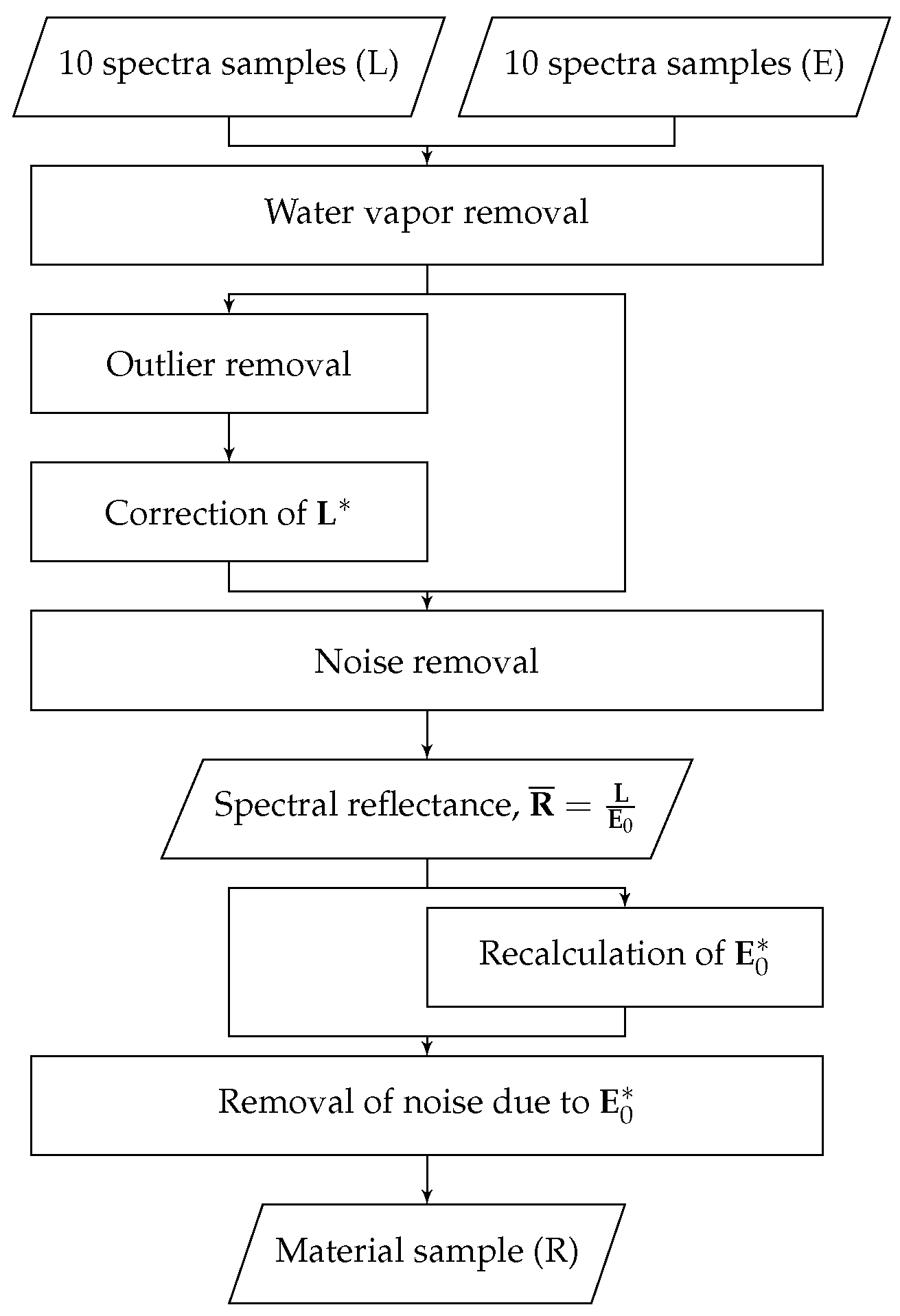
3.2. Data Post-Processing
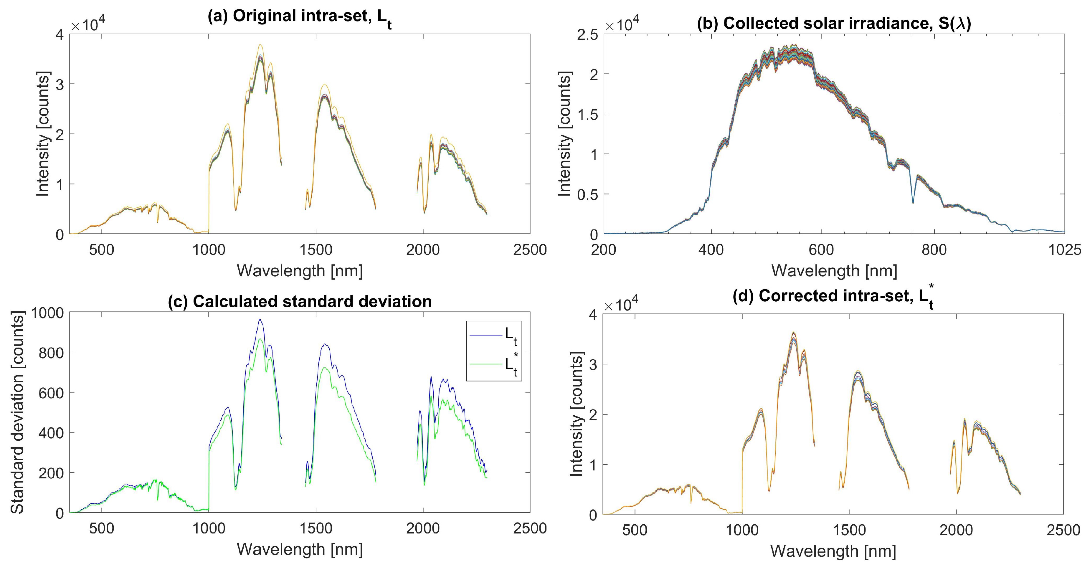
3.2.1. Solar Irradiance Intra-Set Correction
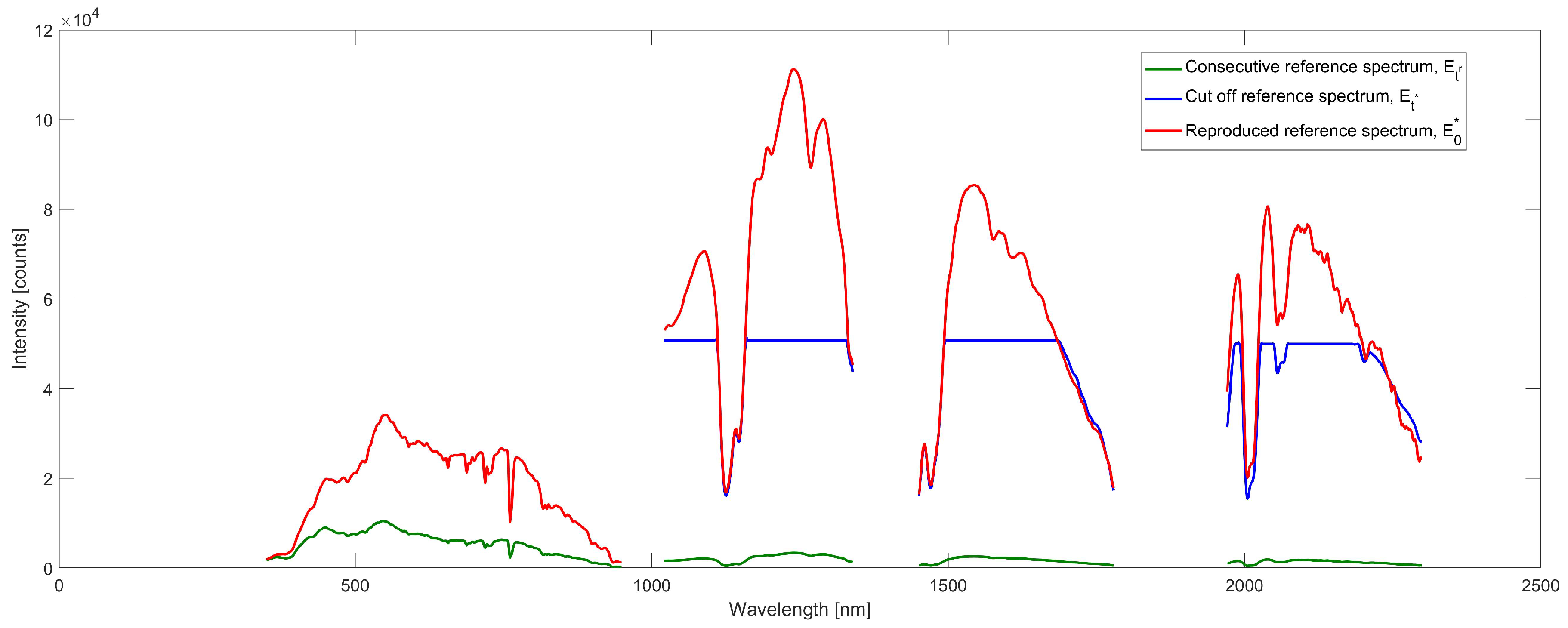
3.2.2. Recalculation of Reference Spectrum Due to Signal Clipping
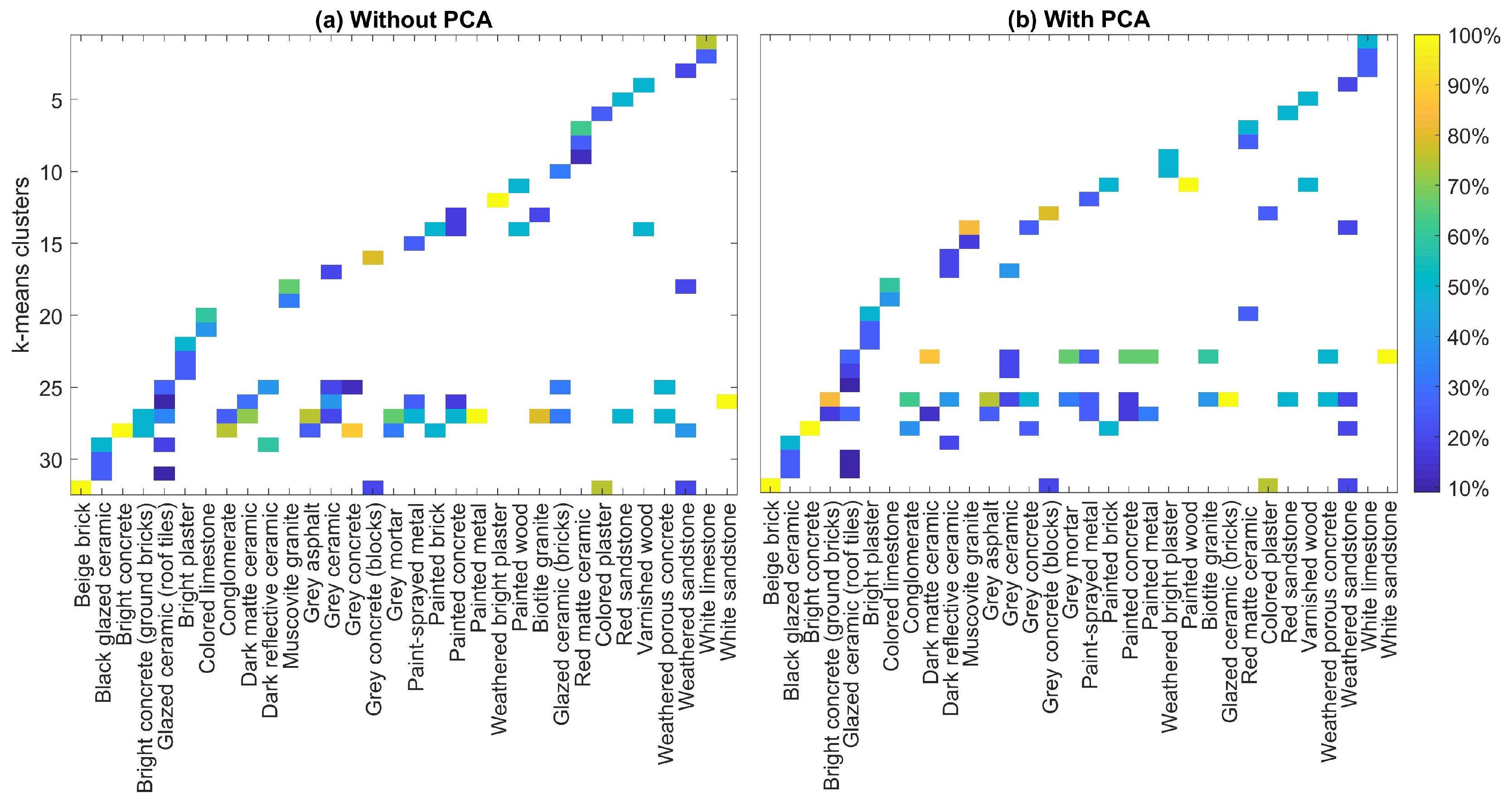
3.3. Material Categorization
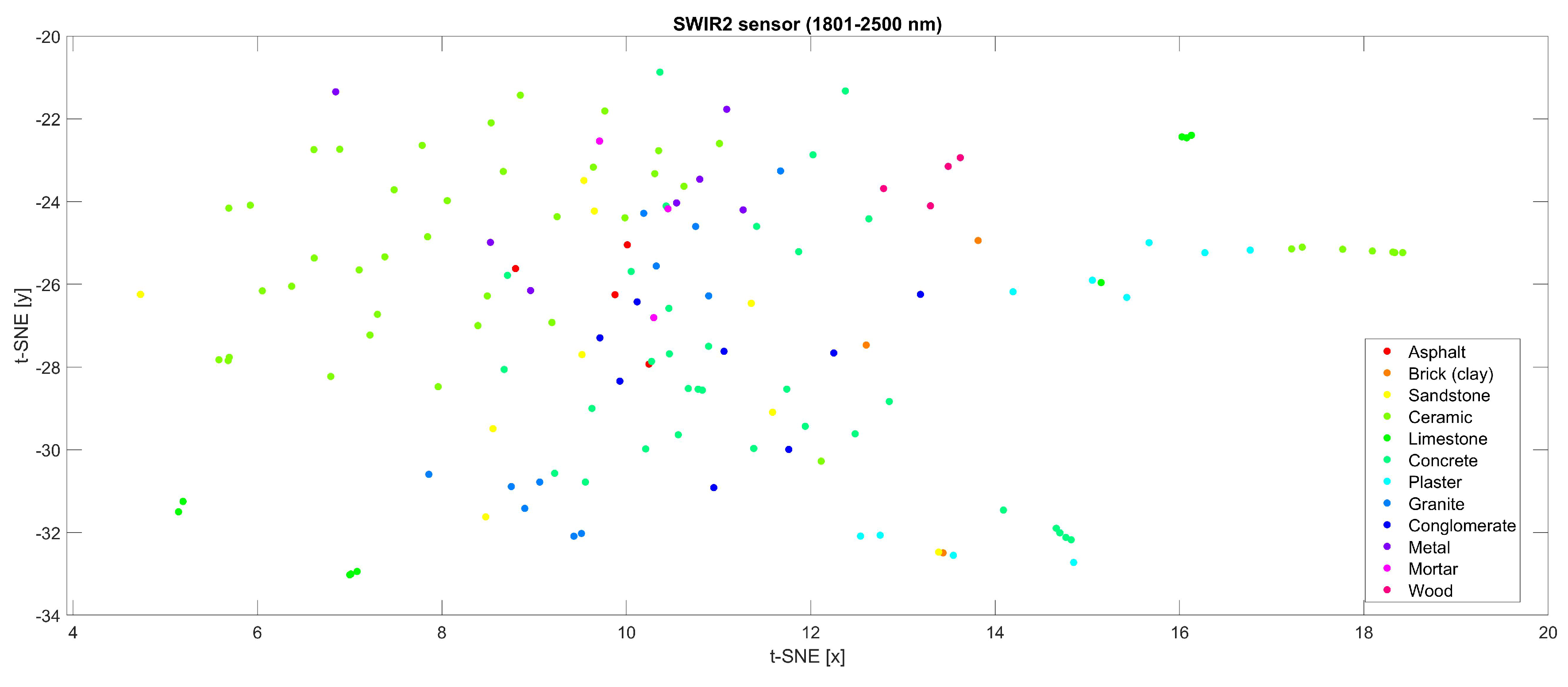
3.3.1. Sample Clustering Based on Spectral Features
3.3.2. Comparison of Spectra
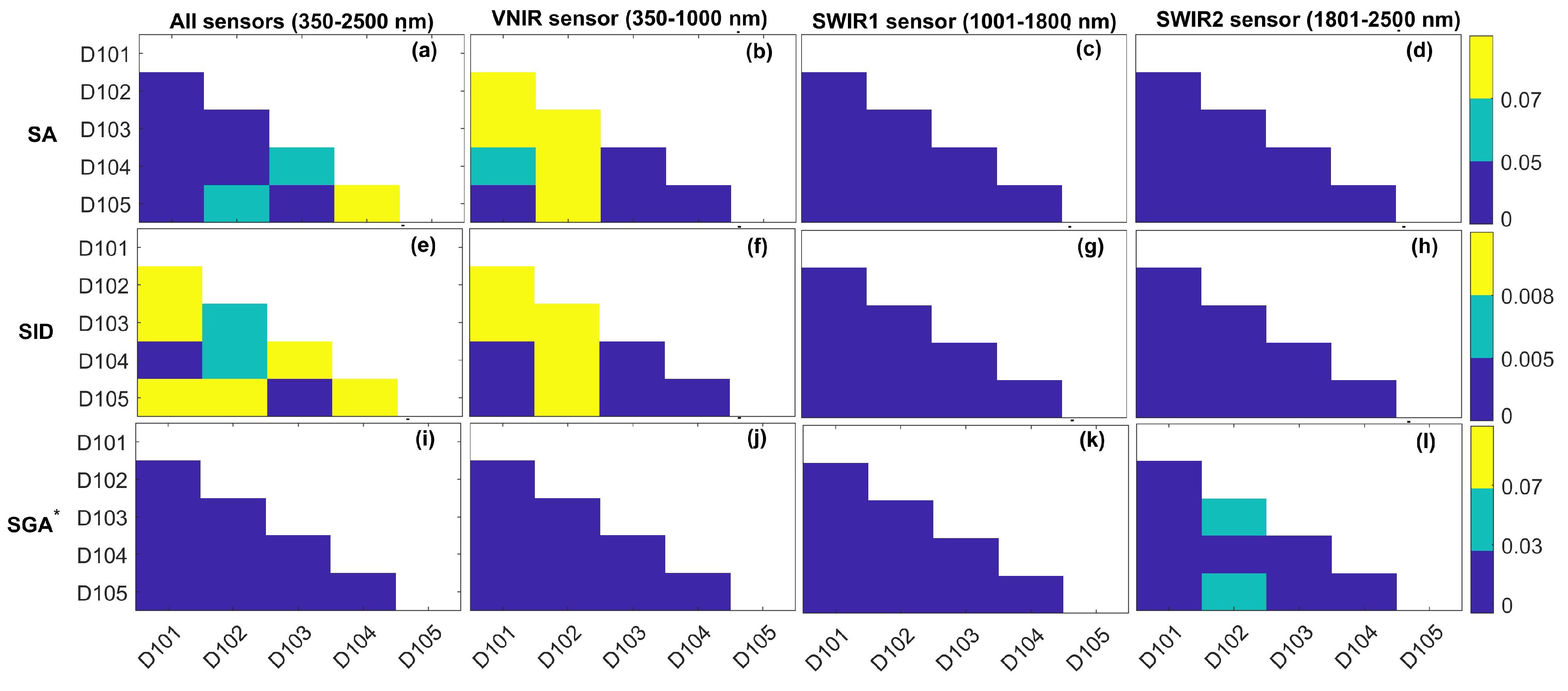
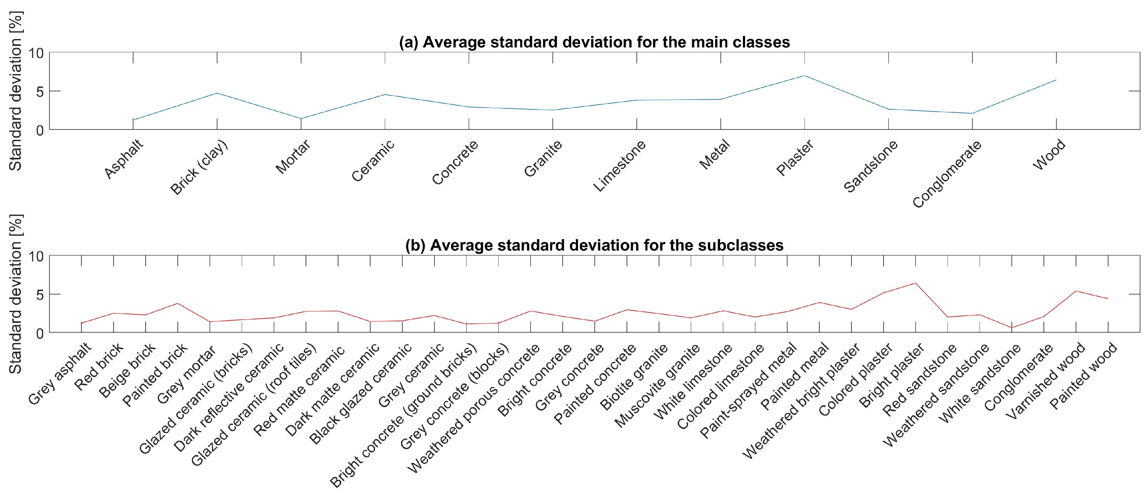
3.3.3. Intra-Class Evaluation
4. Results and Discussion
4.1. Material Samples
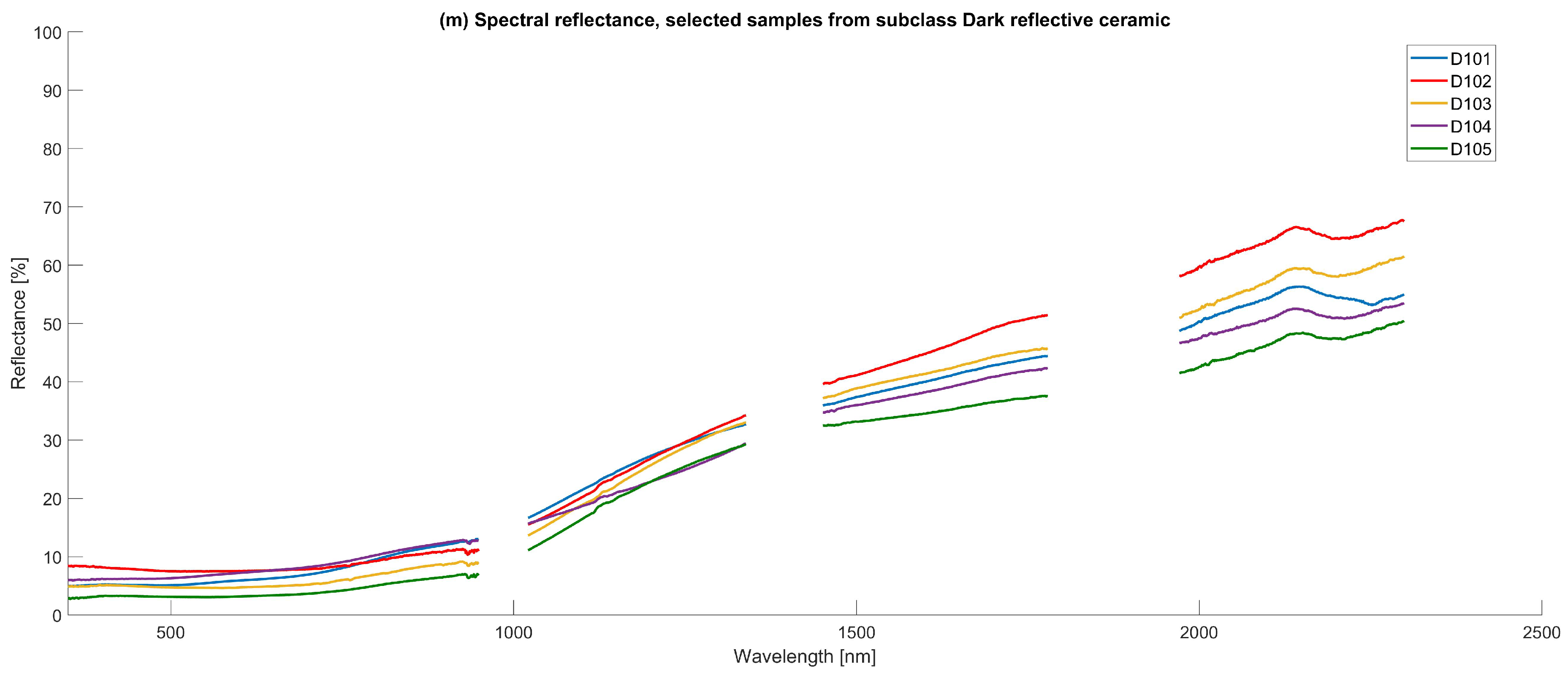
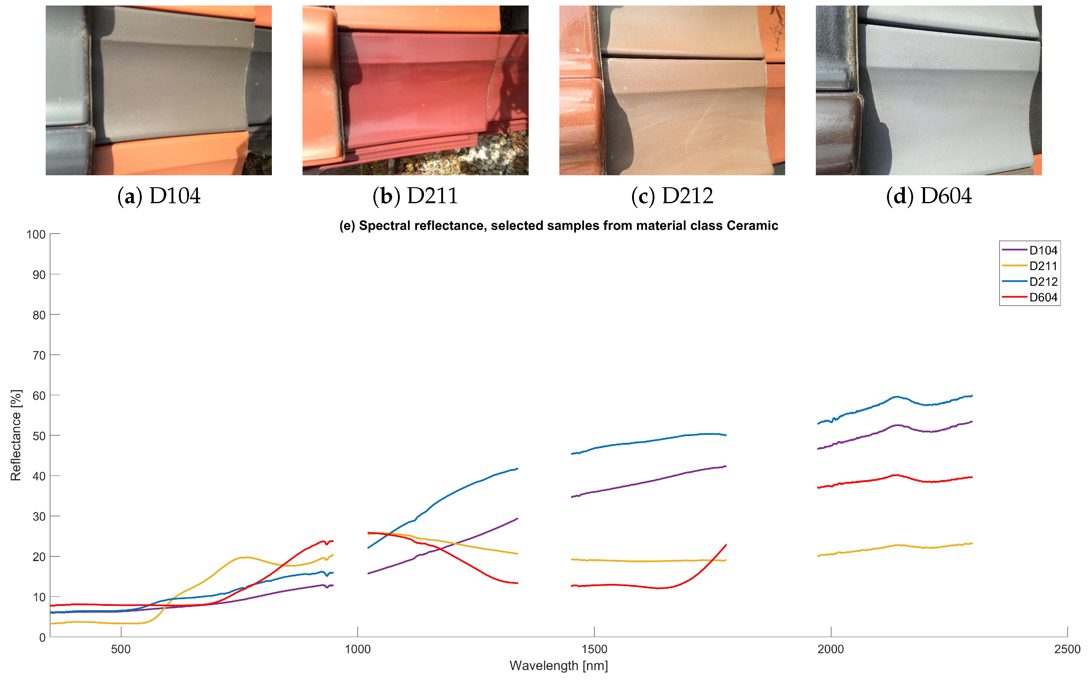
4.1.1. Ceramic
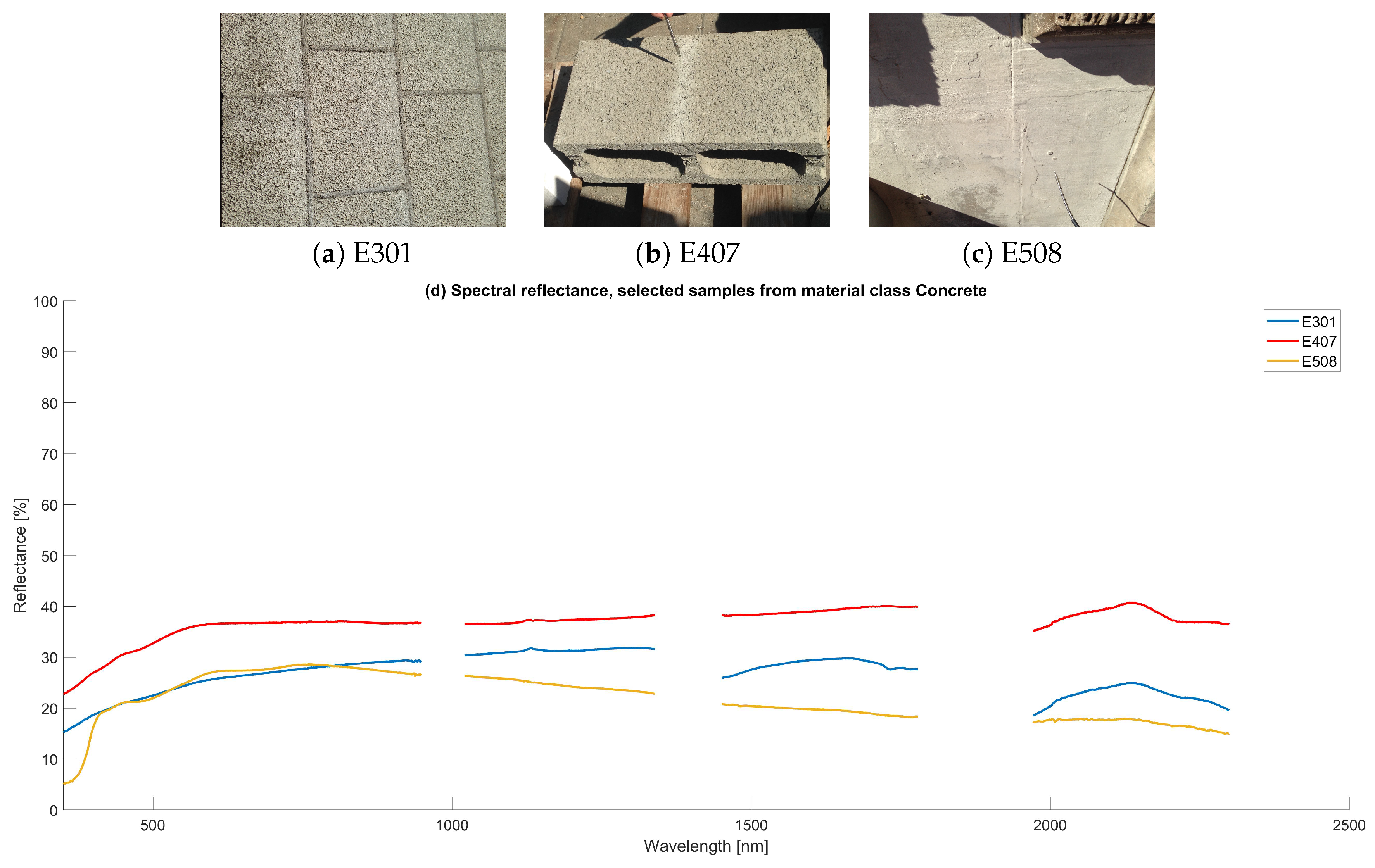
4.1.2. Concrete
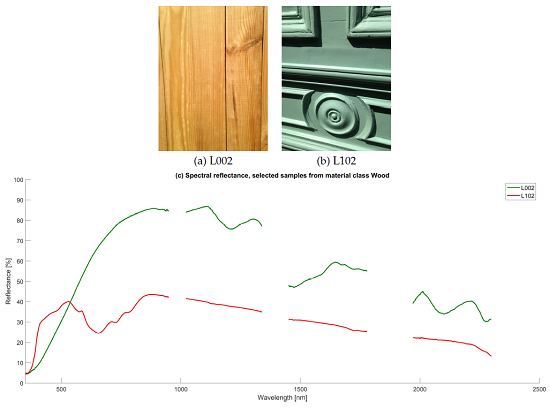
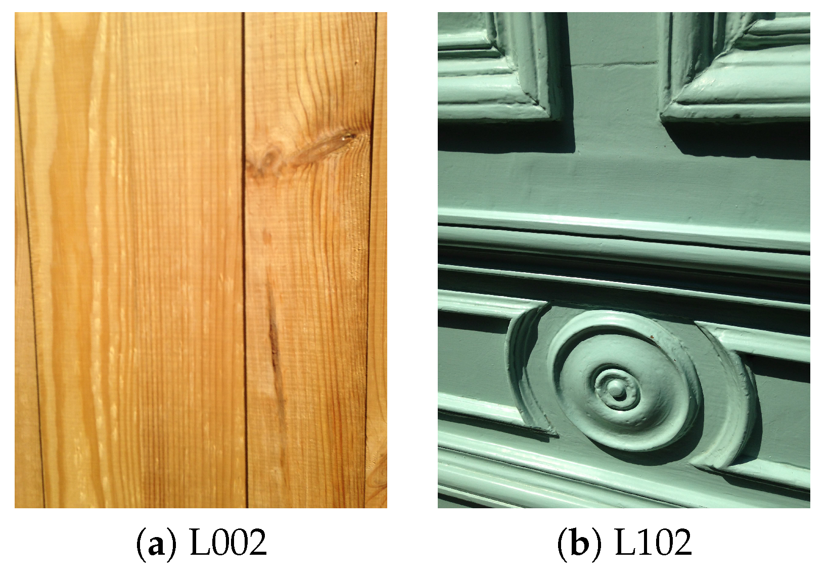
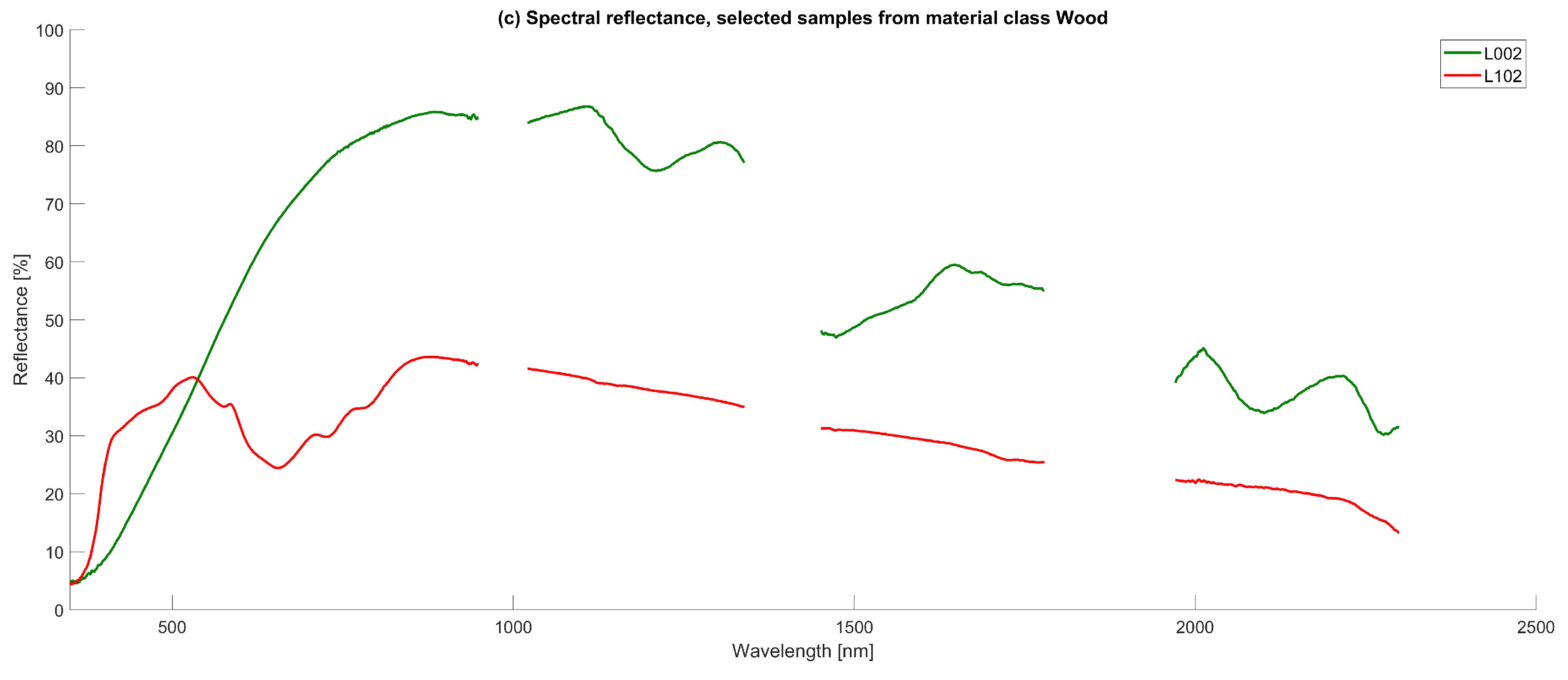
4.1.3. Wood
4.2. Spectral Similarity with Existing Spectral Libraries
4.3. Intra-Class Assessment
4.4. Discussion
5. Conclusions
Author Contributions
Funding
Acknowledgments
Conflicts of Interest
Appendix A. Further Material Samples
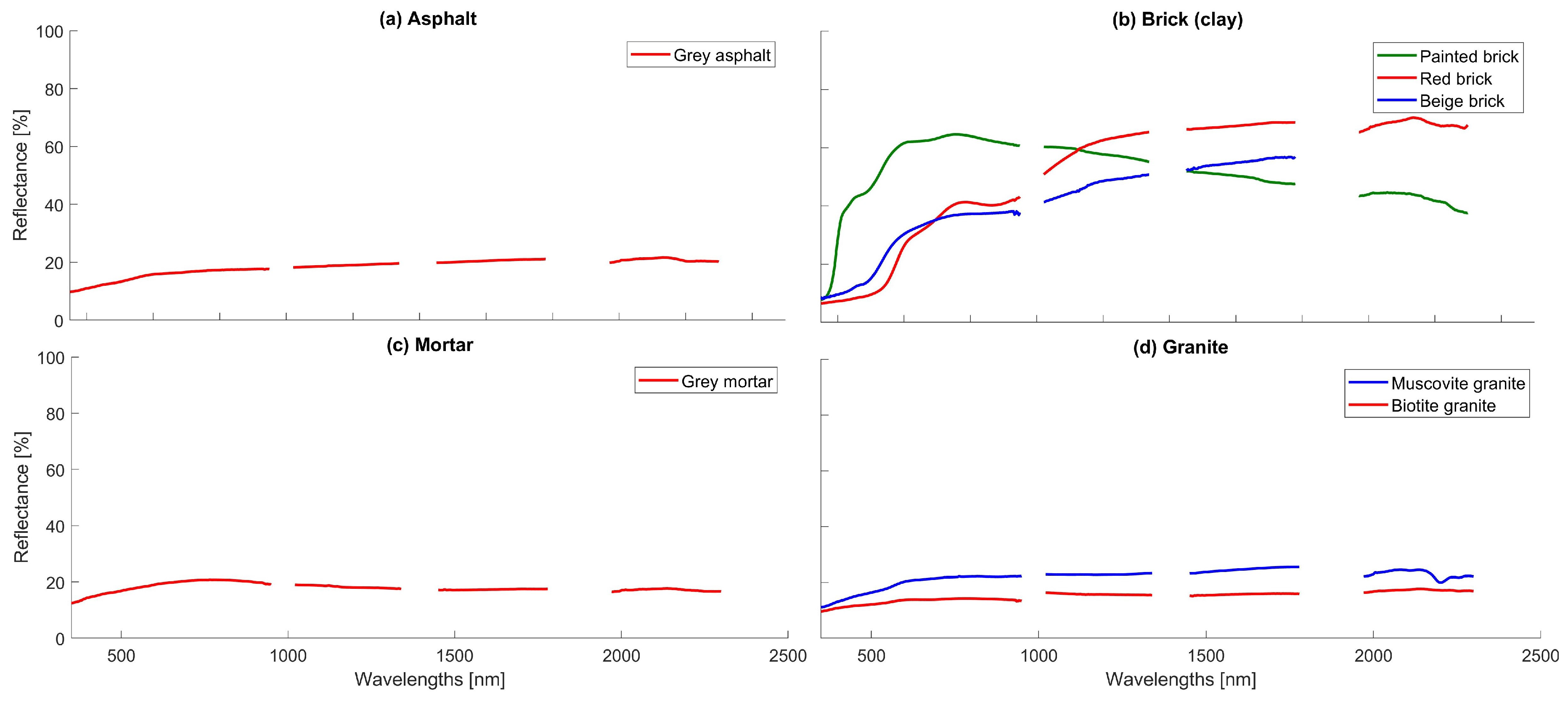
Appendix A.1. Asphalt

Appendix A.2. Brick (Clay)
Appendix A.3. Mortar
Appendix A.4. Granite
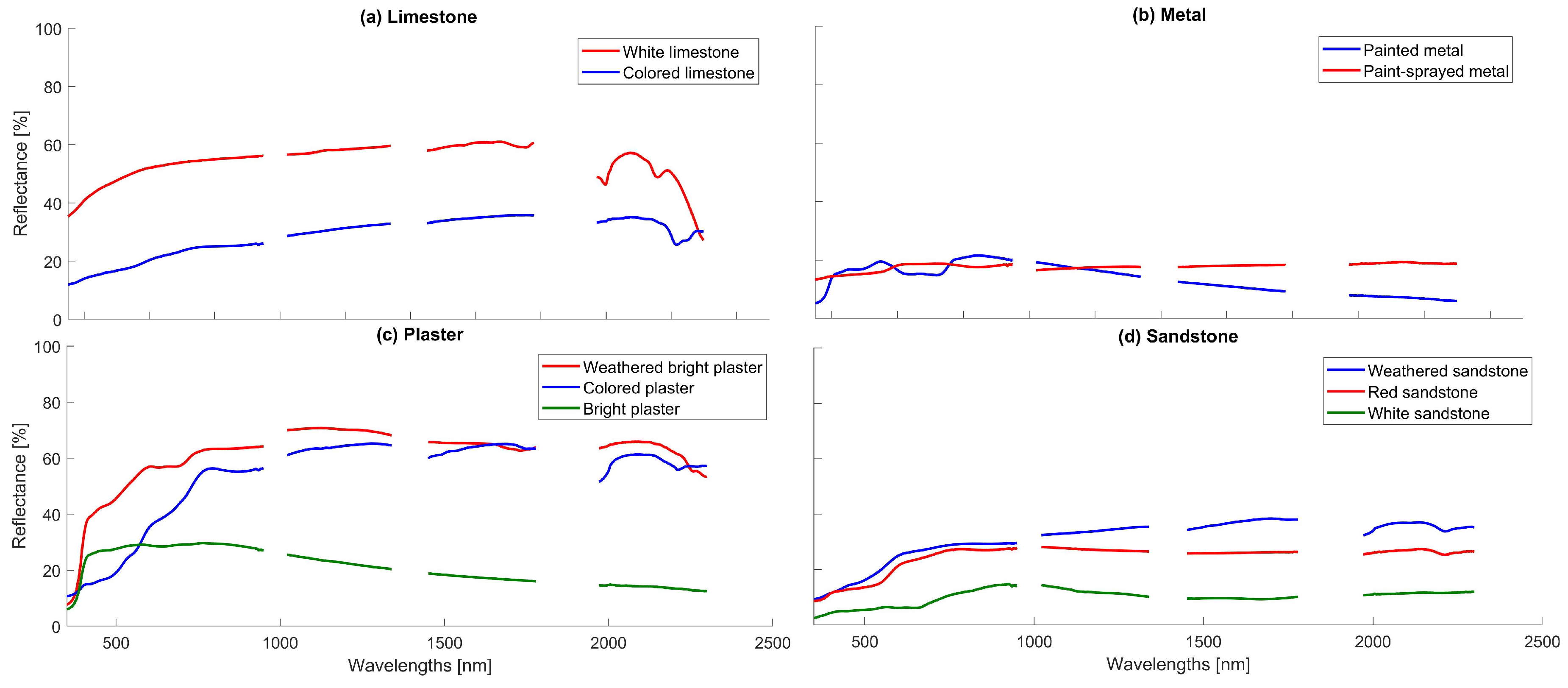
Appendix A.5. Limestone

Appendix A.6. Metal
Appendix A.7. Plaster
Appendix A.8. Sandstone
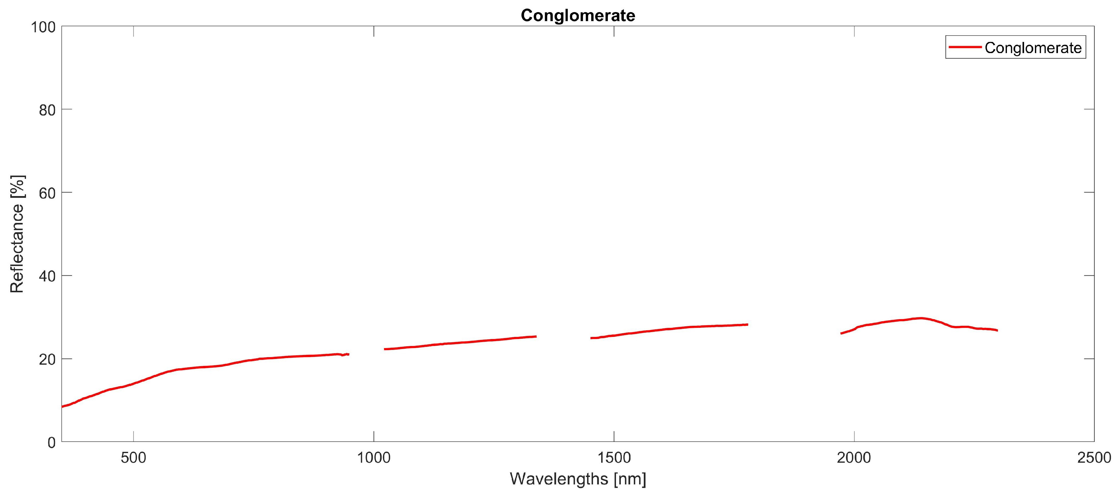
Appendix A.9. Conglomerate

Appendix B. KLUM Material Samples

| Index | Class | Subclass | Usage | Color | Surface Structure/Texture/Coating | Status |
|---|---|---|---|---|---|---|
| A001 | Asphalt | Grey asphalt | Ground | Grey | Fine roughness | Weathered |
| A002 | Asphalt | Grey asphalt | Ground | Grey | Fine roughness | Weathered |
| A003 | Asphalt | Grey asphalt | Ground | Grey | Fine roughness | Weathered |
| A004 | Asphalt | Grey asphalt | Ground | Grey | Fine roughness | Weathered |
| B001 | Brick (clay) | Red brick | Facade | Red | Fine roughness | New |
| B002 | Brick (clay) | Red brick | Facade | Red | Fine roughness | New |
| B003 | Brick (clay) | Red brick | Facade | Red | Fine roughness | New |
| B004 | Brick (clay) | Red brick | Ground | Red | Fine roughness | Weathered |
| B005 | Brick (clay) | Red brick | Facade | Red | Smooth | New |
| B006 | Brick (clay) | Red brick | Facade | Red | Bare; smooth | New |
| B007 | Brick (clay) | Red brick | Facade | Red | Bare; smooth | New |
| B008 | Brick (clay) | Red brick | Facade | Red | Bare; smooth | New |
| B101 | Brick (clay) | Beige brick | Facade | Beige | Smooth | Weathered |
| B102 | Brick (clay) | Beige brick | Facade | Beige | Smooth | Weathered |
| B103 | Brick (clay) | Beige brick | Facade | Beige | Smooth | Weathered |
| B104 | Brick (clay) | Beige brick | Facade | Beige | Fine roughness | Weathered |
| B201 | Brick (clay) | Painted brick | Facade | Grey | Fine roughness; painted | Weathered |
| B202 | Brick (clay) | Painted brick | Facade | Beige | Smooth; painted | New |
| C001 | Mortar | Grey mortar | Facade | Grey | Fine roughness | New |
| C002 | Mortar | Grey mortar | Facade | Grey | Fine roughness | New |
| C003 | Mortar | Grey mortar | Facade | Grey | Fine roughness | New |
| D001 | Ceramic | Glazed ceramic (bricks) | Facade | Red | Glazed; smooth; reflective | New |
| D002 | Ceramic | Glazed ceramic (bricks) | Facade | Red | Glazed; smooth; reflective | New |
| D003 | Ceramic | Glazed ceramic (bricks) | Facade | Red | Glazed; smooth; reflective | New |
| D004 | Ceramic | Glazed ceramic (bricks) | Facade | Red | Glazed; smooth; reflective | Weathered |
| D101 | Ceramic | Dark reflective ceramic | Facade | Black | Smooth; reflective | New |
| D102 | Ceramic | Dark reflective ceramic | Facade | Black | Smooth; reflective | New |
| D103 | Ceramic | Dark reflective ceramic | Roof | Grey | Smooth; reflective | New |
| D104 | Ceramic | Dark reflective ceramic | Roof | Grey | Smooth; reflective | New |
| D105 | Ceramic | Dark reflective ceramic | Roof | Grey | Smooth; reflective | New |
| D201 | Ceramic | Glazed ceramic (roof tiles) | Roof | Red | Glazed; smooth; reflective | New |
| D202 | Ceramic | Glazed ceramic (roof tiles) | Roof | Red | Glazed; smooth; reflective | New |
| D203 | Ceramic | Glazed ceramic (roof tiles) | Roof | Red | Glazed; smooth; reflective | New |
| D204 | Ceramic | Glazed ceramic (roof tiles) | Roof | Red | Glazed; smooth; reflective | New |
| D205 | Ceramic | Glazed ceramic (roof tiles) | Roof | Red | Glazed; smooth; reflective | New |
| D206 | Ceramic | Glazed ceramic (roof tiles) | Roof | Red | Glazed; smooth; reflective | New |
| D207 | Ceramic | Glazed ceramic (roof tiles) | Roof | Brown | Glazed; smooth; reflective | New |
| D208 | Ceramic | Glazed ceramic (roof tiles) | Roof | Red | Glazed; smooth; reflective | New |
| D209 | Ceramic | Glazed ceramic (roof tiles) | Roof | Red | Glazed; smooth; reflective | New |
| D210 | Ceramic | Glazed ceramic (roof tiles) | Roof | Red | Glazed; smooth; reflective | New |
| D211 | Ceramic | Glazed ceramic (roof tiles) | Roof | Red | Glazed; smooth; reflective | New |
| D212 | Ceramic | Glazed ceramic (roof tiles) | Roof | Beige | Glazed; smooth; reflective | New |
| D301 | Ceramic | Red matte ceramic | Roof | Red | Smooth; matte | New |
| D302 | Ceramic | Red matte ceramic | Roof | Red | Smooth; matte | New |
| D303 | Ceramic | Red matte ceramic | Roof | Red | Smooth; matte | New |
| D304 | Ceramic | Red matte ceramic | Roof | Red | Smooth; matte | New |
| D305 | Ceramic | Red matte ceramic | Roof | Red | Smooth; matte | New |
| D306 | Ceramic | Red matte ceramic | Roof | Red | Fine roughness; matte | New |
| D307 | Ceramic | Red matte ceramic | Roof | Red | Fine roughness; matte | New |
| D308 | Ceramic | Red matte ceramic | Roof | Red | Fine roughness; matte | New |
| D401 | Ceramic | Dark matte ceramic | Ground | Grey | Smooth; matte | New |
| D402 | Ceramic | Dark matte ceramic | Roof | Black | Smooth; matte | New |
| D403 | Ceramic | Dark matte ceramic | Roof | Black | Fine roughness; matte | New |
| D404 | Ceramic | Dark matte ceramic | Roof | Grey | Fine roughness; matte | New |
| D405 | Ceramic | Dark matte ceramic | Roof | Grey | Fine roughness; matte | New |
| D406 | Ceramic | Dark matte ceramic | Roof | Brown | Fine roughness; matte | New |
| D407 | Ceramic | Dark matte ceramic | Roof | Brown | Fine roughness; matte | New |
| D501 | Ceramic | Black glazed ceramic | Roof | Black | Glazed; smooth | New |
| D502 | Ceramic | Black glazed ceramic | Roof | Black | Glazed; smooth; reflective | New |
| D503 | Ceramic | Black glazed ceramic | Roof | Black | Glazed; smooth; reflective | New |
| D504 | Ceramic | Black glazed ceramic | Roof | Black | Glazed; smooth; reflective | New |
| D601 | Ceramic | Grey ceramic | Facade | Grey | Uneven | New |
| D602 | Ceramic | Grey ceramic | Roof | Grey | Smooth; reflective | New |
| D603 | Ceramic | Grey ceramic | Roof | Grey | Smooth; reflective | New |
| D604 | Ceramic | Grey ceramic | Roof | Grey | Smooth; reflective | New |
| D605 | Ceramic | Grey ceramic | Ground | Grey | Smooth | Weathered |
| E001 | Concrete | Bright concrete (ground bricks) | Ground | Grey | Fine roughness | Weathered |
| E002 | Concrete | Bright concrete (ground bricks) | Ground | Brown | Fine roughness | Weathered |
| E003 | Concrete | Bright concrete (ground bricks) | Ground | Grey | Fine roughness | Weathered |
| E004 | Concrete | Bright concrete (ground bricks) | Ground | Grey | Fine roughness | Weathered |
| E005 | Concrete | Bright concrete (ground bricks) | Ground | Brown | Fine roughness | Weathered |
| E006 | Concrete | Bright concrete (ground bricks) | Ground | Grey | Fine roughness; cracked | Weathered |
| E007 | Concrete | Bright concrete (ground bricks) | Ground | Brown | Mossy; smooth | Weathered |
| Index | Material | Subclass | Usage | Color | Surface Structure/Texture/Coating | Status |
|---|---|---|---|---|---|---|
| E101 | Concrete | Grey concrete (blocks) | Ground | Grey | Bare; porous | New |
| E102 | Concrete | Grey concrete (blocks) | Ground | Grey | Bare; porous | New |
| E103 | Concrete | Grey concrete (blocks) | Ground | Grey | Bare; porous | New |
| E104 | Concrete | Grey concrete (blocks) | Ground | Grey | Bare; porous | New |
| E105 | Concrete | Grey concrete (blocks) | Ground | Grey | Smooth; uneven | New |
| E201 | Concrete | Weathered porous concrete | Facade | Grey | Porous; uneven | Weathered |
| E202 | Concrete | Weathered porous concrete | Facade | Grey | Porous; uneven | Weathered |
| E203 | Concrete | Weathered porous concrete | Facade | Beige | Fine roughness; porous | Weathered |
| E204 | Concrete | Weathered porous concrete | Facade | Grey | Burnt; porous; uneven | Weathered |
| E301 | Concrete | Bright concrete | Facade | Grey | Bare; porous | Weathered |
| E302 | Concrete | Bright concrete | Facade | Grey | Bare; porous | Weathered |
| E303 | Concrete | Bright concrete | Facade | Beige | Bare; porous | Weathered |
| E304 | Concrete | Bright concrete | Ground | Grey | Fine roughness; uneven | New |
| E305 | Concrete | Bright concrete | Ground | Grey | Fine roughness; uneven | New |
| E401 | Concrete | Grey concrete | Ground | Grey | Fine roughness | Weathered |
| E402 | Concrete | Grey concrete | Facade | Grey | Fine roughness; porous | Weathered |
| E403 | Concrete | Grey concrete | Facade | Grey | Bare; smooth | Weathered |
| E404 | Concrete | Grey concrete | Ground | Grey | Bare; fine roughness | Weathered |
| E405 | Concrete | Grey concrete | Ground | Grey | Bare; porous | New |
| E406 | Concrete | Grey concrete | Ground | Grey | Bare; porous | New |
| E407 | Concrete | Grey concrete | Ground | Grey | Bare; porous | New |
| E408 | Concrete | Grey concrete | Ground | Grey | Smooth | New |
| E409 | Concrete | Grey concrete | Ground | Grey | Fine roughness | New |
| E501 | Concrete | Painted concrete | Facade | Grey | Painted; fine roughness | Weathered |
| E502 | Concrete | Painted concrete | Facade | White | Painted; fine roughness | Weathered |
| E503 | Concrete | Painted concrete | Facade | Grey | Painted; smooth | Weathered |
| E504 | Concrete | Painted concrete | Facade | Grey | Painted; popcorn | New |
| E505 | Concrete | Painted concrete | Facade | Grey | Painted; smooth | New |
| E506 | Concrete | Painted concrete | Facade | Blue | Painted; popcorn | New |
| E507 | Concrete | Painted concrete | Facade | Grey | Painted; popcorn | New |
| E508 | Concrete | Painted concrete | Facade | White | Painted; smooth | Weathered |
| F001 | Granite | Biotite granite | Facade | Blue | Glazed; smooth; reflective | New |
| F002 | Granite | Biotite granite | Ground | Brown | Glazed; smooth | New |
| F003 | Granite | Biotite granite | Facade | Grey | Smooth | Weathered |
| F004 | Granite | Biotite granite | Facade | Grey | Fine roughness | Weathered |
| F005 | Granite | Biotite granite | Facade | Red | Glazed; smooth; reflective | New |
| F006 | Granite | Biotite granite | Facade | Grey | Glazed; smooth | New |
| F007 | Granite | Biotite granite | Ground | Red | Glazed; smooth; reflective | Weathered |
| F008 | Granite | Biotite granite | Facade | Grey | Smooth | New |
| F101 | Granite | Muscovite granite | Facade | Grey | Glazed; reflective; smooth | Weathered |
| F102 | Granite | Muscovite granite | Facade | Red | Glazed; reflective; smooth | New |
| F103 | Granite | Muscovite granite | Facade | Red | Glazed; smooth | Weathered |
| F104 | Granite | Muscovite granite | Ground | Red | Smooth | Weathered |
| F105 | Granite | Muscovite granite | Ground | Red | Glazed; smooth | Weathered |
| F106 | Granite | Muscovite granite | Facade | Grey | Fine roughness; uneven | Weathered |
| F107 | Granite | Muscovite granite | Facade | Red | Glazed; smooth | New |
| F108 | Granite | Muscovite granite | Ground | Grey | Uneven | Weathered |
| G001 | Limestone | White limestone | Facade | White | Uneven | Weathered |
| G002 | Limestone | White limestone | Ground | White | Smooth | Weathered |
| G003 | Limestone | White limestone | Ground | White | Smooth | Weathered |
| G004 | Limestone | White limestone | Ground | White | Smooth | Weathered |
| G101 | Limestone | Colored limestone | Ground | Red | Fine roughness | Weathered |
| G102 | Limestone | Colored limestone | Ground | Red | Fine roughness | Weathered |
| G103 | Limestone | Colored limestone | Ground | Red | Fine roughness | Weathered |
| G104 | Limestone | Colored limestone | Ground | Grey | Smooth | New |
| G105 | Limestone | Colored limestone | Ground | Grey | Smooth | New |
| H001 | Metal | Paint-sprayed metal | Facade | Black | Paint-sprayed; smooth; reflective | New |
| H002 | Metal | Paint-sprayed metal | Facade | Grey | Paint-sprayed; reflective; uneven | New |
| H003 | Metal | Paint-sprayed metal | Facade | Grey | Paint-sprayed; reflective; fine roughness | New |
| H004 | Metal | Paint-sprayed metal | Facade | Grey | Paint-sprayed; smooth; reflective | Weathered |
| H005 | Metal | Paint-sprayed metal | Facade | Grey | Paint-sprayed; smooth; reflective | Weathered |
| H006 | Metal | Paint-sprayed metal | Roof | Grey | Paint-sprayed; smooth; reflective | New |
| H007 | Metal | Paint-sprayed metal | Roof | Red | Paint-sprayed; smooth; reflective | New |
| H101 | Metal | Painted metal | Facade | Blue | Painted; smooth | Weathered |
| H102 | Metal | Painted metal | Facade | Green | Painted; smooth | Weathered |
| H103 | Metal | Painted metal | Facade | Blue | Painted; corrugated; fine roughness | Weathered |
| I001 | Plaster | Weathered bright plaster | Facade | White | Fine roughness | Weathered |
| I002 | Plaster | Weathered bright plaster | Facade | White | Popcorn | Weathered |
| I003 | Plaster | Weathered bright plaster | Facade | Grey | Fine roughness | Weathered |
| I101 | Plaster | Colored plaster | Facade | Pink | Smooth | Weathered |
| I102 | Plaster | Colored plaster | Facade | Green | Smooth | Weathered |
| I103 | Plaster | Colored plaster | Facade | Red | Smooth | Weathered |
| I104 | Plaster | Colored plaster | Facade | White | Fine roughness | Weathered |
| Index | Material | Subclass | Usage | Color | Surface Structure/Texture/Coating | Status |
|---|---|---|---|---|---|---|
| I201 | Plaster | Bright plaster | Facade | White | Fine roughness | New |
| I202 | Plaster | Bright plaster | Facade | Yellow | Popcorn | New |
| I203 | Plaster | Bright plaster | Facade | Beige | Corrugated; uneven | New |
| I204 | Plaster | Bright plaster | Facade | Beige | Smooth | Weathered |
| I205 | Plaster | Bright plaster | Facade | White | Smooth | Weathered |
| J001 | Sandstone | Red sandstone | Facade | Red | Fine roughness | New |
| J002 | Sandstone | Red sandstone | Facade | Red | Uneven | Weathered |
| J003 | Sandstone | Red sandstone | Facade | Red | Uneven | Weathered |
| J004 | Sandstone | Red sandstone | Facade | Red | Fine roughness | Weathered |
| J101 | Sandstone | Weathered sandstone | Facade | Red | Natural; uneven | Weathered |
| J102 | Sandstone | Weathered sandstone | Facade | Red | Natural; uneven | Weathered |
| J103 | Sandstone | Weathered sandstone | Facade | Red | Uneven | Weathered |
| J104 | Sandstone | Weathered sandstone | Facade | Red | Natural; smooth | Weathered |
| J105 | Sandstone | Weathered sandstone | Facade | Red | Natural; uneven | Weathered |
| J106 | Sandstone | Weathered sandstone | Facade | Yellow | Fine roughness | Weathered |
| J201 | Sandstone | Beige sandstone | Facade | Beige | Smooth | New |
| J202 | Sandstone | Beige sandstone | Facade | Beige | Smooth | New |
| K001 | Conglomerate | Conglomerate | Ground | Brown | Bare; fine roughness | Weathered |
| K002 | Conglomerate | Conglomerate | Facade | Grey | Uneven | Weathered |
| K003 | Conglomerate | Conglomerate | Facade | Grey | Uneven | Weathered |
| K004 | Conglomerate | Conglomerate | Facade | Grey | Uneven | Weathered |
| K005 | Conglomerate | Conglomerate | Facade | Grey | Bare; uneven | Weathered |
| K006 | Conglomerate | Conglomerate | Ground | Brown | Uneven | Weathered |
| K007 | Conglomerate | Conglomerate | Ground | Brown | Uneven | Weathered |
| K008 | Conglomerate | Conglomerate | Ground | Brown | Bare; uneven | Weathered |
| K009 | Conglomerate | Conglomerate | Facade | Brown | Smooth | Weathered |
| K010 | Conglomerate | Conglomerate | Facade | Brown | Uneven | Weathered |
| K011 | Conglomerate | Conglomerate | Ground | Brown | Fine roughness | Weathered |
| L001 | Wood | Varnished wood | Facade | Brown | Varnished; smooth | Weathered |
| L002 | Wood | Varnished wood | Facade | Brown | Varnished; smooth | New |
| L101 | Wood | Painted wood | Facade | White | Painted; smooth | New |
| L102 | Wood | Painted wood | Facade | Green | Painted; smooth | Weathered |
| L103 | Wood | Painted wood | Facade | White | Painted; smooth | Weathered |
| L104 | Wood | Painted wood | Facade | Green | Painted; smooth | New |
| L105 | Wood | Painted wood | Facade | Blue | Painted; smooth | Weathered |
References
- Kolbe, T.H. Representing and exchanging 3D city models with CityGML. In 3D Geo-Information Sciences; Springer: Berlin/Heidelberg, Germany, 2009; pp. 15–31. ISBN 978-3-540-87394-5. [Google Scholar]
- Nouvel, R.; Bahu, J.M.; Kaden, R.; Kaempf, J.; Cipriano, P.; Lauster, M.; Häfele, K.H.; Munoz, E.; Tournaire, O.; Casper, E. Development of the CityGML application domain extension energy for urban energy simulation. In Proceedings of the Building Simulation 2015—14th Conference of the International Building Performance Simulation Association, Hyderabad, India, 7–9 December 2015; pp. 559–564. [Google Scholar]
- Kaden, R.; Kolbe, T.H. City-wide total energy demand estimation of buildings using semantic 3D city models and statistical data. In Proceedings of the 8th International 3D GeoInfo Conference, Istanbul, Turkey, 27–29 November 2013; pp. 163–171. [Google Scholar]
- Kottler, B.; Burkard, E.; Bulatov, D.; Haraké, L. Physically-Based Thermal Simulation of Large Scenes for Infrared Imaging. In Proceedings of the 14th International Conference on Compute Graphics Theory and Applications, Prague, Czech Republic, 25–27 February 2019; pp. 1–12. [Google Scholar]
- Xiong, X.; Zhou, F.; Bai, X.; Xue, B.; Sun, C. Semi-automated infrared simulation on real urban scenes based on multi-view images. Opt. Express 2016, 24, 11345–11375. [Google Scholar] [CrossRef] [PubMed]
- Feng, X.; Myint, S.W. Exploring the effect of neighboring land cover pattern on land surface temperature of central building objects. Build. Environ. 2016, 95, 346–354. [Google Scholar] [CrossRef]
- Oke, T.R. The energetic basis of the urban heat island. Q. J. R. Meteorol. Soc. 1982, 108, 1–24. [Google Scholar] [CrossRef]
- Ward, K.; Lauf, S.; Kleinschmit, B.; Endlicher, W. Heat waves and urban heat islands in Europe: A review of relevant drivers. Sci. Total Environ. 2016, 569, 527–539. [Google Scholar] [CrossRef] [PubMed]
- Ilehag, R.; Bulatov, D.; Helmholz, P.; Belton, D. Classification and representation of commonly used roofing material using multisensorial aerial data. Int. Arch. Photogramm. Remote Sens. Spat. Inf. Sci. 2018, 42, 217–224. [Google Scholar] [CrossRef]
- Santamouris, M.; Synnefa, A.; Karlessi, T. Using advanced cool materials in the urban built environment to mitigate heat islands and improve thermal comfort conditions. Sol. Energy 2011, 85, 3085–3102. [Google Scholar] [CrossRef]
- Susca, T.; Gaffin, S.R.; Dell’Osso, G.R. Positive effects of vegetation: Urban heat island and green roofs. Environ. Pollut. 2011, 159, 2119–2126. [Google Scholar] [CrossRef] [PubMed]
- Kyriakodis, G.E.; Santamouris, M. Using reflective pavements to mitigate urban heat island in warm climates-Results from a large scale urban mitigation project. Urban Clim. 2018, 24, 326–339. [Google Scholar] [CrossRef]
- Ilehag, R.; Schenk, A.; Hinz, S. Concept for classifying facade elements based on material, geometry and thermal radiation using multimodal UAV remote sensing. Int. Arch. Photogramm. Remote Sens. Spat. Inf. Sci. 2017, 42, 145–151. [Google Scholar] [CrossRef]
- González-Aguilera, D.; Lagüela, S.; Rodríguez-Gonzálvez, P.; Hernández-López, D. Image-based thermographic modeling for assessing energy efficiency of buildings façades. Energy Build. 2013, 65, 29–36. [Google Scholar] [CrossRef]
- Fokaides, P.A.; Kalogirou, S.A. Application of infrared thermography for the determination of the overall heat transfer coefficient (U-Value) in building envelopes. Appl. Energy 2011, 88, 4358–4365. [Google Scholar] [CrossRef]
- Breiman, L. Random forests. Mach. Learn. 2001, 45, 5–32. [Google Scholar] [CrossRef]
- Cortes, C.; Vapnik, V. Support-vector networks. Mach. Learn. 1995, 20, 273–297. [Google Scholar] [CrossRef]
- Franke, J.; Roberts, D.A.; Halligan, K.; Menz, G. Hierarchical multiple endmember spectral mixture analysis (MESMA) of hyperspectral imagery for urban environments. Remote Sens. Environ. 2009, 113, 1712–1723. [Google Scholar] [CrossRef]
- van der Linden, S.; Okujeni, A.; Canters, F.; Degerickx, J.; Heiden, U.; Hostert, P.; Priem, F.; Somers, B.; Thiel, F. Imaging spectroscopy of urban environments. Surv. Geophys. 2018, 40, 1–18. [Google Scholar] [CrossRef]
- Nasarudin, N.E.M.; Shafri, H.Z.M. Development and utilization of urban spectral library for remote sensing of urban environment. J. Urban Environ. Eng. 2011, 5, 44–56. [Google Scholar] [CrossRef]
- Baldridge, A.M.; Hook, S.J.; Grove, C.I.; Rivera, G. The ASTER spectral library version 2.0. Remote Sens. Environ. 2009, 113, 711–715. [Google Scholar] [CrossRef]
- Clark, R.N.; Swayze, G.A.; Wise, R.; Livo, K.E.; Hoefen, T.; Kokaly, R.F.; Sutley, S.J. USGS Digital Spectral Library Splib06a; U.S. Geological Survey: Reston, VA, USA, 2007. [CrossRef]
- Heiden, U.; Segl, K.; Roessner, S.; Kaufmann, H. Determination of robust spectral features for identification of urban surface materials in hyperspectral remote sensing data. Remote Sens. Environ. 2007, 111, 537–552. [Google Scholar] [CrossRef] [Green Version]
- Herold, M.; Roberts, D.A.; Gardner, M.E.; Dennison, P.E. Spectrometry for urban area remote sensing-Development and analysis of a spectral library from 350 to 2400 nm. Remote Sens. Environ. 2004, 91, 304–319. [Google Scholar] [CrossRef]
- Kotthaus, S.; Smith, T.E.L.; Wooster, M.J.; Grimmond, C.S.B. Derivation of an urban materials spectral library through emittance and reflectance spectroscopy. ISPRS J. Photogramm. Remote Sens. 2014, 94, 194–212. [Google Scholar] [CrossRef] [Green Version]
- Sobrino, J.A.; Sòria, G.; Romaguera, M.; Cuenca, J. Desirex 2008: Estudio de la isla de calor en la Ciudad de Madrid. Revista de Teledetección 2009, 31, 80–92. [Google Scholar]
- Ben-Dor, E.; Levin, N.; Saaroni, H. A spectral based recognition of the urban environment using the visible and near-infrared spectral region (0.4–1.1 μm). A case study over Tel-Aviv, Israel. Int. J. Remote Sens. 2001, 22, 2193–2218. [Google Scholar] [CrossRef]
- Jalali, S.; Parapari, D.M.; Mahdavinejad, M.J. Analysis of Building Facade Materials Usage Pattern in Tehran. Adv. Eng. Forum 2019, 32, 46–62. [Google Scholar] [CrossRef]
- Sánchez, J.; Quirós, E. Semiautomatic detection and classification of materials in historic buildings with low-cost photogrammetric equipment. J. Cult. Herit. 2017, 25, 21–30. [Google Scholar] [CrossRef]
- Ilehag, R.; Weinmann, M.; Schenk, A.; Keller, S.; Jutzi, B.; Hinz, S. Revisiting existing classification approaches for building materials based on hyperspectral data. Int. Arch. Photogramm. Remote Sens. Spat. Inf. Sci. 2017, 42, 65–71. [Google Scholar] [CrossRef]
- Fairbarn, K.G., Jr. Visible-Near Infrared (VNIR) and Shortwave Infrared (SWIR) Spectral Variability of Urban Materials. Master’s Thesis, Naval Postgraduate School, Monterey, CA, USA, 2013. [Google Scholar]
- Price, J.C. Examples of high resolution visible to near-infrared reflectance sand a standardized collection for remote sensing studies. Int. J. Remote Sens. 1995, 16, 993–1000. [Google Scholar] [CrossRef]
- Heiden, U.; Roessner, S.; Segl, K.; Kaufmann, H. Analysis of spectral signatures of urban surfaces for their identification using hyperspectral HyMap data. In Proceedings of the IEEE/ISPRS Joint Workshop on Remote Sensing and Data Fusion over Urban Areas (Cat. No. 01EX482), Rome, Italy, 8–9 November 2001; pp. 173–177. [Google Scholar]
- Herold, M.; Roberts, D.A. Spectral characteristics of asphalt road aging and deterioration: Implications for remote-sensing applications. Appl. Opt. 2005, 44, 4327–4334. [Google Scholar] [CrossRef] [PubMed]
- Sobrino, J.A.; Oltra-Carrió, R.; Jiménex-Muñoz, J.C.; Julien, Y.; Sòria, G.; Franch, B.; Mattar, C. Emissivity mapping over urban areas using a classification-based approach: Application to the Dual-use European Security IR Experiment (DESIREX). Int. J. Appl. Earth Obs. Geoinf. 2012, 18, 141–147. [Google Scholar] [CrossRef]
- Kokaly, R.F.; Clark, R.N.; Swayze, G.A.; Livo, K.E.; Hoefen, T.M.; Pearson, N.C.; Wise, R.A.; Benzel, W.M.; Lowers, H.A.; Driscoll, R.L.; et al. USGS Spectral Library Version 7: U.S. Geological Survey Data Series 1035; U.S. Geological Survey: Reston, VA, USA, 2017. [CrossRef]
- Abel, J.S.; Smith, J.O. Restoring a clipped signal. In Proceedings of the ICASSP 91: 1991 International Conference on Acoustics, Speech, and Signal Processing, Toronto, ON, Canada, 14–17 May 1991; pp. 1745–1748. [Google Scholar]
- Keshava, N. Distance metrics and band selection in hyperspectral processing with applications to material identification and spectral libraries. IEEE Trans. Geosci. Remote Sens. 2002, 42, 1552–1565. [Google Scholar] [CrossRef]
- Kruse, F.A.; Lefkoff, A.B.; Boardman, J.W.; Heidebrecht, K.B.; Shapiro, A.T.; Barloon, P.J.; Goetz, A.F.H. The Spectral Image Processing System (SIPS)—Interactive Visualization and Analysis of Imaging spectrometer Data. Remote Sens. Environ. 1993, 44, 145–163. [Google Scholar] [CrossRef]
- Chang, C.I. Hyperspectral Imaging: Techniques for Spectral Detection and Classification; Kluwer Academic/Plenum Publishers: New York, NY, USA, 2003; Volume 1, ISBN 0-306-47483-2. [Google Scholar]
- Angelopoulou, E.; Kee, S.W.; Bajcsy, R. Spectral gradients: A material descriptor invariant to geometry and incident illumination. In Proceedings of the Seventh IEEE International Conference on Computer Vision, Kerkyra, Greece, 20–27 September 1999; pp. 861–867. [Google Scholar]
- Robila, S. An investigation of spectral metrics in hyperspectral image preprocessing for classification. In Proceeding of the Geospatial Goes Global: From Your Neighborhood to the Whole Planet, ASPRS Annual Conference, Baltimore, MD, USA, 7–11 March 2005; pp. 7–11. [Google Scholar]
- Lloyd, S.P. Least Squares Quantization in PCM. IEEE Trans. Inf. Theory 1982, 28, 129–137. [Google Scholar] [CrossRef]
- Pearson, K., III. On lines and planes of closest fit to systems of points in space. Lond. Edinb. Dublin Philos. Mag. J. Sci. 1901, 2, 559–572. [Google Scholar] [CrossRef]
- van der Maaten, L.; Hinton, G. Visualizing data using t-SNE. J. Mach. Learn. Res. 2008, 9, 2579–2605. [Google Scholar]
- Le Bris, A.; Chehata, N.; Briottet, X.; Paparoditis, N. Spectral Band Selection for Urban Material Classification Using Hyperspectral Libraries. ISPRS Ann. Photogramm. Remote Sens. Spat. Inf. Sci. 2016, 3, 33–40. [Google Scholar] [CrossRef]


| Spectral Library | Study Area | Content | Spectral Range | Data Acquisition |
|---|---|---|---|---|
| Ben-Dor et al. [27] | Tel-Aviv, Israel | 55 samples, of which: 11 facade 16 ground 2 roof | VNIR | Airborne In situ |
| Heiden et al. [33] & [23] | Dresden and Potsdam, Germany | 32 samples, of which: 8 ground 13 roof | VNIR SWIR | Airborne In situ |
| Herold et al. [24]Santa Barbara spectral library* | Santa Barbara, CA, USA | 26 samples, of which: 9 ground 3 roof | VNIR SWIR | Airborne In situ |
| Baldridge et al. [21] ASTER spectral library* | Various locations, USA | 3420 samples, of which: 28 facade 10 ground 18 roof | VNIR SWIR TIR | Laboratory |
| Sobrino et al. [26] DESIREX | Madrid, Spain | 27 samples, of which: 3 facade 18 ground 1 roof | VNIR SWIR MWIR LWIR | Airborne In situ |
| Nasarudin et al. [20] | Serdang, Malaysia | 15 samples, of which: 7 roof 3 ground | VNIR SWIR | In situ |
| Kotthaus et al. [25] LUMA-SLUM spectral library* | London, UK | 74 samples, of which: 48 facade 9 ground 17 roof | VNIR SWIR LWIR | Laboratory In situ |
| Kokaly et al. [36] USGS Spectral Library Version 7* | Various locations, USA | 2468 samples, of which: 9 facades 15 ground 16 roof | VNIR SWIR LWIR VLWIR | Airborne Laboratory In situ |
| KLUM* | Karlsruhe, Germany | 181 samples, of which: 97 facade 46 ground 38 roof | VNIR SWIR | In situ |
| Material | Class ID | Subclass | Count |
|---|---|---|---|
| Asphalt | A | Grey asphalt | 4 |
| Brick (clay) | B | Red brick | 8 |
| Beige brick | 4 | ||
| Painted brick | 2 | ||
| Mortar | C | Grey mortar | 3 |
| Ceramic | D | Glazed ceramic (bricks) | 4 |
| Dark reflective ceramic | 5 | ||
| Glazed ceramic (roof tiles) | 12 | ||
| Red matte ceramic | 8 | ||
| Dark matte ceramic | 7 | ||
| Black glazed ceramic | 4 | ||
| Grey ceramic | 5 | ||
| Concrete | E | Bright concrete (ground bricks) | 7 |
| Grey concrete (blocks) | 5 | ||
| Weathered porous concrete | 4 | ||
| Bright concrete | 5 | ||
| Grey concrete | 9 | ||
| Painted concrete | 8 | ||
| Granite | F | Biotite granite | 8 |
| Muscovite granite | 8 | ||
| Limestone | G | White limestone | 4 |
| Colored limestone | 5 | ||
| Metal | H | Paint-sprayed metal | 7 |
| Painted metal | 3 | ||
| Plaster | I | Weathered bright plaster | 3 |
| Colored plaster | 4 | ||
| Bright plaster | 5 | ||
| Sandstone | J | Red sandstone | 4 |
| Weathered sandstone | 6 | ||
| White sandstone | 2 | ||
| Conglomerate | K | Conglomerate | 11 |
| Wood | L | Varnished wood | 2 |
| Painted wood | 5 |
| 1. Material | 2. Usage | 3. Color | 4. Surface Structure/Texture/Coating | 5. Status |
|---|---|---|---|---|
| Asphalt | Facade | Beige | Bare | New |
| Brick (clay) | Ground | Black | Burnt | Weathered |
| Ceramic | Roof | Blue | Corrugated | |
| Concrete | Brown | Cracked | ||
| Conglomerate | Green | Fine roughness | ||
| Granite | Grey | Glazed | ||
| Limestone | Pink | Matte | ||
| Metal | Red | Mossy | ||
| Mortar | White | Natural | ||
| Plaster | Yellow | Painted | ||
| Sandstone | Paint-sprayed | |||
| Wood | Popcorn | |||
| Porous | ||||
| Reflective | ||||
| Smooth | ||||
| Uneven | ||||
| Varnished |
© 2019 by the authors. Licensee MDPI, Basel, Switzerland. This article is an open access article distributed under the terms and conditions of the Creative Commons Attribution (CC BY) license (http://creativecommons.org/licenses/by/4.0/).
Share and Cite
Ilehag, R.; Schenk, A.; Huang, Y.; Hinz, S. KLUM: An Urban VNIR and SWIR Spectral Library Consisting of Building Materials. Remote Sens. 2019, 11, 2149. https://doi.org/10.3390/rs11182149
Ilehag R, Schenk A, Huang Y, Hinz S. KLUM: An Urban VNIR and SWIR Spectral Library Consisting of Building Materials. Remote Sensing. 2019; 11(18):2149. https://doi.org/10.3390/rs11182149
Chicago/Turabian StyleIlehag, Rebecca, Andreas Schenk, Yilin Huang, and Stefan Hinz. 2019. "KLUM: An Urban VNIR and SWIR Spectral Library Consisting of Building Materials" Remote Sensing 11, no. 18: 2149. https://doi.org/10.3390/rs11182149