Large Scale Agricultural Plastic Mulch Detecting and Monitoring with Multi-Source Remote Sensing Data: A Case Study in Xinjiang, China

Abstract

Plastic mulching has been widely practiced in crop cultivation worldwide due to its potential to significantly increase crop production. However, it also has a great impact on the regional climate and ecological environment. More importantly, it often leads to unexpected soil pollution due to fine plastic residuals. Therefore, accurately and timely monitoring of the temporal and spatial distribution of plastic mulch practice in large areas is of great interest to assess its impacts. However, existing plastic-mulched farmland (PMF) detecting efforts are limited to either small areas with high-resolution images or coarse resolution images of large areas. In this study, we examined the potential of cloud computing and multi-temporal, multi-sensor satellite images for detecting PMF in large areas. We first built the plastic-mulched farmland mapping algorithm (PFMA) rules through analyzing its spectral, temporal, and auxiliary features in remote sensing imagery with the classification and regression tree (CART). We then applied the PFMA in the dry region of Xinjiang, China, where a water resource is very scarce and thus plastic mulch has been intensively used and its usage is expected to increase significantly in the near future. The experimental results demonstrated that the PFMA reached an overall accuracy of 92.2% with a producer’s accuracy of 97.6% and a user’s accuracy of 86.7%, and the F-score was 0.914 for the PMF class. We further monitored and analyzed the dynamics of plastic mulch practiced in Xinjiang by applying the PFMA to the years 2000, 2005, 2010, and 2015. The general pattern of plastic mulch usage dynamic in Xinjiang during the period from 2000 to 2015 was well captured by our multi-temporal analysis.

1. Introduction

In a broad sense, agriculture using plastic film for crop cultivation can be defined as plasticulture [1]. Since plastic film was used in agriculture in 1948 [2], it has been widely utilized for cultivating crops, fruits, and vegetables. The use of plastic film in agricultural can alleviate the threat of cold, high temperature, wind, insects, drought, and consequently increase crop yield [3]. According to reports, the total area of agriculture plastic film has been expanded at an average rate of 20% per year globally over the last decade [4]. Plastic mulch is playing an increasingly important role in modern agriculture. On one hand, the widespread use of plastic mulch has significantly increased crop yield, which is of great significance for food security [5,6,7]. On the other hand, plastic mulch increases soil temperature and maintains soil moisture, so it alters the exchange of matter and energy between the land surface and the atmosphere including the following aspects [8,9,10]: (i) Plastic mulch can alter surface roughness, leading to more incoming sunlight reflected back to the atmosphere, and increased temperature of the atmosphere. (ii) Plastic mulch can prevent water to evaporate, thus altering water cycles. (iii) Plastic mulch and its inner surface with dew can block the emission of longwave radiation, increasing the temperature of the soil. (iv) Plastic mulch can block gas, such as N₂O, CO₂, and CH_4, the exchange between soil and atmosphere. Moreover, plastic mulch can influence the residual rate of soil organic materials in the soil, inevitably affecting soil microbial and soil ecosystems [11].

At present, the biggest negative impact of plastic mulching might be plastic mulch residues. Plastic mulch is a hydrocarbon polymer compound, mainly made of polyethylene, thus it is very hard to completely degrade under natural conditions [12,13]. Both the Chinese National Environmental Monitoring Centre and the U.S. Environmental Protection Agency listed this compound as a priority for controlling pollutants [14]. According to the survey conducted by The Ministry of Agriculture of the People’s Republic of China (MOA) in the early 1990s, all the plastic-mulched farmland have different levels of residues, with an average residue of 60 kg·hm⁻² and a maximum of 135 kg·hm ⁻². The long-term residue of plastic mulch in the farmland not only destroys the structure of the pellet in the soil, but also affects the soil permeability, reduces soil porosity and water content, and increases soil bulk density and specific gravity [15,16,17]. If the residual amount of plastic mulch becomes too large, crops can have physiological phenomena such as leaf wilting, dead seedlings, premature aging, etc., which will cause the decline of farmland quality, crop reduction, and agricultural operations hindered [15,18,19,20]. Moreover, the residues of plastic mulch in soils may eventually turn into microplastics through environmental degradation [21,22]. In recent years, these problems have become more and more serious, which has already constituted a great threat to the eco-environment and global climate [12,23].

According to statistics from the Chinese Agricultural Yearbooks and National Bureau of Statistics of China (NBSC; Figure 1.), the use of plastic film for agriculture in China increased about two times with an average annual growth rate of about 6% from 1.335 million tons to 2.635 million tons from 2000 to 2015. Among them, the average annual use of plastic mulch accounts for 54.77% in terms of tonnage and 95% in terms of coverage of total plastic film consumed [5]. There are two main types of plastic mulches: Transparent plastic mulch and colored plastic mulch (e.g., white plastic mulch and black plastic mulch), and the transparent plastic mulch account for about 99% in total plastic mulch consumed [24]. There is an urgent need to accurately and timely understand the temporal and spatial distribution of plastic mulch over large areas to provide accurate information about plastic mulch for each relevant organizational unit and application. For example, such information can help industries plan and produce plastic film, organize the recovery of plastic mulch or estimate the number of plastic mulch residues, and can help researchers study land surface temperatures.

By using remote sensing images, it is possible to acquire quantitative and qualitative information about ground objects in a timely and quick manner over large areas [25,26,27]. With remote sensing technology, it is possible to obtain accurate information about plastic mulch areas and their spatial distribution. Recent studies of mapping and monitoring plasticulture farmland mainly concentrate on extracting plastic greenhouse farmland, with very few studies focus on plastic-mulched farmland. Up to date, researches used passive or active remote sensing data to map plasticulture farmland can be divided into two main groups: Pixel-based and object-based classification. For pixel-based plasticulture farmland extraction, Carvajal et al. [28,29] based on pixel-based classifiers to extract plastic greenhouses using QuickBird and IKONOS images. Levin et al. [30] used a 1 m-resolution AISA-ES hyperspectral image to monitor transparent and black plastic greenhouses. Agüera et al. [31,32] developed a pixel-based classification algorithm to identify plastic greenhouses from both Quickbird and IKONOS images. Koc-San [33] tested different pixel-based classifiers to detect glass and plastic greenhouses from WorldView-2 and found that support vector machine method achieved better results. Novelli and Tarantino [34] combined four different indices and pixel-based classification algorithm to detect plastic-covered vineyard with Landsat-8 imagery. Yang et al. [35] mapped plastic greenhouses with medium spatial resolution satellite data. Lanorte et al. [36] proposed a pixel-based approach to estimate agricultural plastic waste with Landsat-8 satellite images. For object-based plasticulture farmland extraction, Tarantino and Figorito [37] successfully mapped plastic-covered vineyards with high spatial resolution true color aerial images. Agüera et al. [38] combined WorldView-2 and Landsat-8 images to map plastic greenhouses with object-based image analysis and a decision tree classification scheme. Nemmaoui et al. [39] identified plastic greenhouses based on multi-temporal and multi-sensor satellite data. Yao and Wang [40] proposed the over-segmentation index (OSI)–under-segmentation index (USI)–error index of total area (ETA)–composite error index (CEI) pattern to extract plastic greenhouses from GaoFen-2 (GF-2) imagery. All these studies mostly used high-resolution images to monitor plastic greenhouses. Although they successfully mapped plasticulture farmland in specific areas with high-resolution images, whether these studies can be extended to other regions still requires careful examination.

However, the spectral and the spatial characteristics of plastic-mulched farmland are very different than those of plastic greenhouses. For example, plastic mulch is mostly used in semi-arid or arid areas and the critical period of monitoring plastic-mulched farmland is very short (from the sowing of crops to their emergence, just about one month), but that is not the case for plastic greenhouses. Monitoring plastic-mulched farmland with remote sensing data has been attracting a great deal of attention in recent years, particularly in China. Wang [41] used multi-angle polarization information to extract plastic-mulched paddy fields over a water background. Lu et al. [24] extracted transparent plastic-mulched landcover with Landsat-5 Thematic Mapper (TM) images and a pixel-based classifier, and later they [42,43] proposed a pixel-based threshold model and the improved spatial attraction model (ISAM) to map large-scale subpixel plastic-mulched landcover from Moderate Resolution Imaging Spectroradiometer (MODIS) imagery. Recently the same team [44] proposed a new object-based image analysis approach to extract plastic-mulched landcover combining Sentinel-1 Synthetic Aperture Radar (SAR) and Sentinel-2 multi-spectral data. Hasituya et al. [45] used spectral features and texture features in Landsat-8 Operational Land Imager (OLI) data to monitor plastic-mulched farmland with different pixel-based classifiers, and later they [46] mapped plastic-mulched farmland with C-Band full polarization SAR data and different pixel-based classifiers. They [10] collected spectra, textures, indices, and thermal features from multi-temporal Landsat-8 imagery to map plastic-mulched farmland with different pixel-based classifiers, and later they [47] used an average local variance (ALV) function and a pixel-based classifier to mapping plastic-mulched farmland with GaoFen-1 (GF-1) satellite imagery. Liu et al. [48] combined full polarimetric RADARSAT-2 data and dual polarimetric (HH, VV) TerraSAR-X data to map plastic-mulched farmland with a pixel-based classifier. These proposed methods mostly focused on single year plastic-mulched farmland mapping in a small spatial extent.

To summarize up, we found that: (i) To date, most researchers focused mainly on single-year plasticulture farmland extraction, rarely on long-term plasticulture farmland mapping; (ii) most current efforts on mapping plasticulture farmland mainly focused on small regions with medium or high-resolution imagery (mostly a single image or several images). Although they successfully mapped plasticulture farmland in their study areas, how to map and monitor plastic-mulched farmland over large regions remains a big challenge.

The Google Earth Engine (GEE) is a cloud-based platform designed to enable petabyte-scale, scientific analysis and visualization of geospatial datasets [49]. GEE provides an integrated environment including a massive data catalog (Landsat 4–8, Sentinel 1–3, et al.) together with thousands of computers for planetary-scale data analysis, and offers a friendly workbench environment to allow interactive algorithm development through JavaScript (or Python) based Application Programming Interface (GEE APIs). Now more and more researchers are using this platform for large-scale land cover and land use change mapping and monitoring. Dong et al. [50] mapped the paddy rice planting area in northeastern Asia with Landsat 8 images on GEE. Xiong et al. [51] obtained the spatial and temporal distributions of cropland in continental Africa with MODIS NDVI (Normalized Difference Vegetation Index) time series data on GEE. Patel et al. [52] extracted the multi-temporal settlement and population on the Indonesian island of Java from Landsat images on GEE. All these studies indicated that cloud computing facilities like GEE have brought a significant transformation in land cover and land use mapping and monitoring.

We propose a new framework to map plastic-mulched farmland and to monitor its dynamics over large areas with the GEE cloud platform using multi-source (Sentinel-2, Landsat 5–8, and MODIS) satellite imagery. It constitutes several steps: (i) Examining the spectral characteristic of PMF and constructing a plastic-mulched farmland index (PMFI); (ii) extracting and selecting classification features; (iii) constructing plastic-mulched farmland mapping algorithm (PFMA) rules with a decision tree classification scheme; and (iv) monitoring plastic-mulched farmland dynamics.

2. Materials

2.1. Study Area

The Xinjiang Uygur Autonomous Region of China is divided into the northern, the eastern and the southern portions by geographical factors (the Tianshan Mountains) and social-economic factors (the number of population), extending from 34°25′N to 48°10′N and from 73°40′E to 96°18′E, with a total land area of 1.66 million km² (Figure 2). This region is located in an arid and semi-arid climate zone, with typical irrigated oasis agriculture. Major plastic mulch crops in this area are cotton, corn, tomatoes, beets, watermelons, vegetables, etc. The total amount of plastic mulch used for cotton is the largest, which accounts for more than 60% of the total plastic mulch use in Xinjiang and all cotton fields are mulched by transparent plastic mulch [53]. The plastic mulch used in the southern Xinjiang and eastern Xinjiang is mainly for soil moisture conservation, while in northern Xinjiang it is also for increasing soil temperature. According to statistics, the annual use of plastic mulch in Xinjiang is about 61.4 kg/hm², and over 84.8% farmland used plastic mulch to cultivating crops [54]. Due to the wide and improper (e.g., the thickness of plastic mulch cannot reach the national standard) use of plastic mulch in Xinjiang and ineffective recovery, soil plastic mulch residue in this area is the largest in China. For example, in the cotton field, 18 kg/hm² of plastic mulch remains in the farmland every year [55,56]. The negative impacts of the residual plastic film, especially the potential hazard have become more and more serious, but have not attracted much attention. There is an urgent need to map and monitor the temporal and spatial distribution of plastic-mulched farmland (PMF) in Xinjiang to help design proper policies to ensure sustainable development in this region.

2.2. Remote Sensing Imagery Data

The best time to detect PMF from space is from the sowing of crops to their emergence because crop leaves will block plastic mulch when they grow up. Due to the vast territory of Xinjiang, the natural conditions of different regions in this area are quite different, which leads to great differences in crop phenology calendars [57]. To accurately identify and extract the information of plastic mulch, we must understand the phenological information of crops covered with plastic mulch in each region. For example, cotton sowing is in early April in the southern, mid-April in the northern, and late April in the eastern Xinjiang (

Table 1. Phenological calendar of cotton in Xinjiang.

Month	April			May			June			July			August			September
Ten-day	E	M	L	E	M	L	E	M	L	E	M	L	E	M	L	E	M	L
Northern Xinjiang
Southern Xinjiang
Eastern Xinjiang

Sowing: blue; Emargence: red; Seeding stage: yellow; Bud stage: green; Blooming period: light brown; Boll opening stage: light green.

). Among these three major cotton-growing areas, the sowing period can vary by 15 to 20 days, but there is little difference between the northern Xinjiang and the eastern Xinjiang (within 5 days). Therefore we divided the study area into two regions by comparing the phenological calendar of crops in Xinjiang. We designated the northern and the eastern Xinjiang as the first region (Zone 1), and the period from mid-April to mid-May was considered as the best identification period for PMF in this region. We treated the southern Xinjiang as the second region (Zone 2) and the period from early April to late April was the best identification period for PMF in this region.

However, due to limited temporal resolutions of medium spatial resolution images and the influence of clouds, it is not feasible to use a single image source for large area PMF extraction. It was necessary to combine multiple source data to cover the entire Xinjiang region. According to the Xinjiang Statistical Yearbook (these yearbooks include various Xinjiang’s social and economic development statistics information, such as the change of crop planting structure, water resource information, and so on), official records of the use of plastic mulch in Xinjiang began in 2015. In order to better obtain the spectral and temporal information of PMF with medium imagery over a large area, we took the Sentinel-2 Multispectral Instrument data (Sentinel-2 MSI) whose temporal resolution is 10 days with one satellite and 5 days with two satellites and spatial resolution is 10 m, which is higher than that of Landsat-8, as the main remote sensing data to model PFMA. However, the Sentinel-2 MSI data was not available until 23 June 2015, so we chose data in 2016 to generate PFMA retrieving rules. At the same time, we applied the PFMA to map PMF in 2000, 2005, 2010, 2015, and 2016 by using Sentinel-2 MSI, Landsat 5-8 top of atmosphere (TOA) Reflectance, and MOD09A1.006 Terra Surface Reflectance data in April, May, July, and August (

Table 2. Characteristics of Sentinel-2 Multispectral Instrument (MSI), Landsat-8 (Operational Land Imager) OLI, Landsat-7 (Enhanced Thematic Mapper Plus) ETM+, Landsat-5 (Thematic Mapper) TM, and MOD09A1.006 bands used in this study.

Sensors	Period	Bands	Use	WaveLength	Resolution	Data Availability
Sentinel-2, MSI	April–May July–August	B2	Blue	490 nm	10 m	23 June 2015 – Now
		B4	Red	664 nm	10 m
		B8	Near Infrared	842 nm	10 m
		B12	Short-wave Infrared 2	2190 nm	20 m
Landsat-8, OLI	April–May July–August	B2	Blue	430–450 nm	30 m	11 April 2013 – Now
		B4	Red	640–670 nm	30 m
		B5	Near Infrared	850–880 nm	30 m
		B7	Short-wave Infrared 2	2110–2290 nm	30 m
Landsat-7, ETM+	April–May July–August	B1	Blue	450–520 nm	30 m	1 January 1999 – Now
		B3	Red	630–690 nm	30 m
		B4	Near Infrared	770–900 nm	30 m
		B7	Short-wave Infrared 2	2090–2350 nm	30 m
Landsat-5, TM	April–May July–August	B1	Blue	450–520 nm	30 m	1 January 1984 – 5 May 2012
		B3	Red	630–690 nm	30 m
		B4	Near Infrared	760–900 nm	30 m
		B7	Short-wave Infrared 2	2080–2350 nm	30 m
MOD09A1.006	April–May July–August	sur_refl_b03		459–479 nm	500 m	5 March 2000 – Now
		sur_refl_b01		620–670nm	500 m
		sur_refl_b02		841–876 nm	500 m
		sur_refl_b07		2105–2155 nm	500 m

). The number of images used for mapping PMF in independent years was shown in

Table 3. The number of images used for mapping plastic-mulched farmland (PMF) in this study.

Years	Regions	Period	Sentinel-2 MSI	Landsat-8 OLI	Landsat-7 ETM+	Landsat-5 TM	MOD09A1 V6	The Number of Images
2016	Zone 1	April	284	106	95		3	488
		July	354	96	99		4	553
	Zone 2	May	251	134	127		3	515
		August	606	112	90		4	812
2015	Zone 1	April		110	99		4	213
		July		104	92		4	200
	Zone 2	May		129	121		3	254
		August		127	121		4	252
2010	Zone 1	April			83	92	4	179
		July			75	81	4	160
	Zone 2	May			80	117	3	200
		August			79	94	4	177
2005	Zone 1	April			84	58	4	146
		July			71	48	4	123
	Zone 2	May			91	47	3	141
		August			94	25	4	123
2000	Zone 1	April			37	21	3	61
		July			34	45	4	83
	Zone 2	May			59	44	3	106
		August			72	37	4	113

.

2.3. Other Auxiliary Data

In addition to using remote sensing imagery data, we also used other data (

Table 4. The information of the auxiliary data.

Name	Time	Institution
Shuttle Radar Topography Mission (SRTM) 30 m	2000	NASA/USGS
National Land Use Dataset (NLUD) 30 m	2000–2016	Chinese Academy of Sciences
China Agricultural Yearbooks	2000–2015	Ministry of Agriculture of the People’s Republic of China
Annual by Province in Xinjiang	2000–2015	National Bureau of Statistics of China
Xinjiang Statistical Yearbook	2016–2017	Statistic Bureau of Xinjiang Uygur Autonomous Region

) to help monitoring PMF. We used the cropland layer from the National Land Use Dataset (NLUD, which was developed by the Chinese Academy of Sciences through visual interpretation of Landsat data) to confine our analysis of plastic mulch coverage within agriculture zones to minimize confusion with other land features. The SRTM (Shuttle Radar Topography Mission 30 m) data was used to generate slope information, which would be used to help monitoring PMF. Statistics data from the Xinjiang Statistical Yearbook were used to analyze the spatial distribution of PMF in Xinjiang.

3. Methods

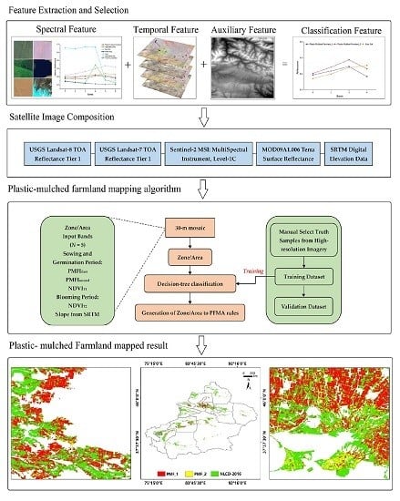
3.1. Overview of the Methodology

An overview of the proposed methodology is shown in Figure 3. First, we look up the spectral curve of the mainly ground objects (plastic mulch, vegetation cover, saline-alkali soil, water body, impervious surface, bare soil, and so on) in the study area in the U.S. Geological Survey (USGS) spectral database [58], the wavelengths covering the range from 0.35 to 2.5 µm (from analytical spectral devices (ASD) field portable spectrometers). In contrast to the spectral curve from mainly ground objects after, we chose the spectral, temporal, and auxiliary features as the classification features (Section 3.2). Second, we built a 30-m image mosaic (five-bands) for each zone (in Zone 1 for May and July in 2016, in Zone 2 for April and August in 2016 in Xinjiang) combining Sentinel-2 MSI, Landsat 7-8 TOA Reflectance, and MOD09A1.006 Terra Surface Reflectance cloudless data (Section 3.3). Third, we obtained training samples from the reference samples’ repository (Section 3.4) to train a decision tree classifier and generate PFMA rules (Section 3.5). Fourth, we ensembled and deployed PFMA on the GEE, and applied it in each zone (Section 3.6). Finally, we applied a majority filter (the number of neighboring cells to use in the kernel of the filter is four in this paper, the kernel of the filter will be the four direct (orthogonal) neighbors to the present cell) to remove salt-pepper noise from the decision tree classification (pixel-based classification). We collected validation samples and validated the classification results in each zone.

3.2. Classification Feature Extraction and Selection

Classification feature extraction and selection plays an important role in imagery classification [45]. To understand the spectral differences of different ground objects in the study area, we looked up their spectral curves in the USGS spectral database. By comparing the spectral curves, we established two ratio indices as the spectral features to extract PMF. Moreover, we found the spectral characteristics of PMF are easily confused with wet soil, building, and mountain shadows, and we used time-phase features and other auxiliary features from the remote sensing imagery to remove the influence of wet soils, buildings, and mountain shadows on the identification of PMF, which will be detailed in the following sections.

3.2.1. Spectral Feature Extraction and Selection

According to the field investigation, the spectral information of PMF was often a mixture of plastic mulch, bare soil, and dew. In terms of spectral features, bare soil and PMF show good separability with water body, vegetation, saline-alkali soil, impervious surface, etc. [45]. Although the spectral features of bare soil and PMF are similar, they can be well separated in the visible and short-wave infrared bands. From the visible to near-infrared bands, because the plastic mulch is a white or transparent non-polarized thermoplastic composed of polyethylene, the spectral reflectance of PMF largely depends on the background soils. Thus, the shape of the spectral reflectance curve of PMF is often similar to that of bare soils. However, because plastic mulch can reduce the bare soil roughness, PMF is much brighter and smoother than bare soils. Therefore, the spectral reflectance of PMFs was higher than those of bare soils in the visible and near-infrared bands (Figure 4). In the short-wave infrared band, the plastic mulch and water body show obvious absorption characteristics [30]. At night, the internal temperature of the plastic mulch is higher than outside, saturated water vapor often condenses into dew on the inner surface of the plastic mulch. In Xinjiang, the temperature gap between day and night can reach more than 10 °C, so this phenomenon is more prominent. Consequently, the reflectance of PMFs in the short-wave infrared was often lower than that of bare soils, but significantly higher than water (Figure 4).

Based on the differences of spectral characteristics between PMF and other ground objects (vegetation cover, saline-alkali soil, water body, impervious surface, bare soil, etc.) in the visible to short-wave infrared bands, the plastic-mulched farmland index (PMFI) can be constructed. The blue band (Sentinel-2 MSI, 0.452–0.512 μm) was sensitive to water and chlorophyll. Similar to the water body and vegetation cover, PMF and bare soil had low reflectance in the blue band, but snow had a high reflectance in this band. The near-infrared band (Sentinel-2 MSI, 0.851–0.879 μm) was sensitive to vegetation cover. Vegetation cover, saline-alkali soil, and snow had high reflectance whereas PMF, bare soil, impervious surface, and water body had low reflectance in this band. Since the short-wave infrared (Sentinel-2 MSI, 2.107–2.294 μm) located at the water and polyethylene absorption bands, the reflectance of PMF, bare soil, and saline-alkali soil was higher than other objects in this band, and the reflectance of saline-alkali soil was observably higher than PMF and bare soil in this band. The reflectance of PMF was lower than bare soil in the short-wave infrared band, which was completely different than in the visible bands. Based on the above discussion, we proposed two PMFIs:

$$PMF{I}_{first}=\frac{{\rho }_{SWIR}}{{\rho }_{NIR}},$$

(1)

$$PMF{I}_{second}=\frac{{\rho }_{SWIR}}{{\rho }_{Blue}},$$

(2)

where ρ_SWIR (Sentinel-2 MSI, 2.107–2.294 μm) is reflectance in the short-wave infrared band, ρ_NIR (Sentinel-2 MSI, 0.851–0.879 μm) is reflectance in the near-infrared band, and ρ_Blue (Sentinel-2 MSI, 0.452–0.512 μm) is reflectance in the blue band. Since almost all plastic mulches used in the study area were transparent, the PMF showed either blue or grayish blue colors in the arbitrary color composite of Sentinel-2 MSI (R = SWIR2, G = NIR, and B = Blue; Figure 5), depending on the thickness of the plastic mulch, crop growing condition, soil types, soil moisture, and condensed water. Therefore, we divided the PMF into two types: Plastic-mulched farmland_1 (PMF1, blue in Figure 5b) and plastic-mulched farmland_2 (PMF2, grayish blue in Figure 5d). According to field investigation, we found that PMF1 was almost all plastic mulches with a thickness reaching the national standard (GB4455–1994 and GB13735–1992 stipulates that the thickness of the plastic mulch used in China cannot be less than 8 μm), or had abundant condensed water on the inner side, and less bare soil put over the plastic mulch. PMF2 was almost all plastic mulches with a thickness lower than the national standard (ranging from 3 to 6 μm, in Xinjiang), or had a handful of condensed water on the inner side, and a large amount of bare soil put over the plastic mulch to prevent it being blown away by strong winds.

3.2.2. Temporal Feature Extraction and Selection

In the key phenological identification period of PMF, their values can be easily confused with mountain shadows, building shadows, and wet soils. The growth conditions of crops in different periods are needed to distinguish PMF from mountain shadows, building shadows, and wet soils. NDVI is an index that is widely used for evaluating vegetation conditions over the land surface [59,60,61]. Therefore, we choose the NDVI value in different periods as the phase characteristics of PMF extraction. The NDVI can be calculated as follows:

$$NDVI=\frac{{\rho }_{NIR}-{\rho }_{Red}}{{\rho }_{NIR}+{\rho }_{Red}},$$

(3)

where ρ_NIR is reflectance in the infrared band, and ρ_Red is reflectance in the red band. According to the phenological calendar of mulched crops, such as cotton and corn, the median NDVI (can indicate the growth of the vegetation over a period of time) in the periods of May (NDVI_T1) and July (NDVI_T2) was calculated as the time-phased characteristics of the Zone 1, and the median NDVI in the periods of April (NDVI_T1) and August (NDVI_T2) was calculated as the time-phased characteristics of the Zone 2 (The number of images used for calculating the median NDVI was shown in Table 3). Besides, the multi-temporal NDVI can also eliminate the influence of greenhouses and low-tunnel cropland for mapping PMF in Xinjiang, because the crops are inside of the greenhouse or low-tunnel, so its spectral characteristics are close to plastic film, and their NDVI values are relatively low (the maximum NDVI in a year is in July or August and lower than 0.4).

3.2.3. Auxiliary Feature Extraction and Selection

From April to May, soils on mountain slopes may become wet due to snowmelt, easy to be confused with PMF. Therefore, we derived slope information from the shuttle radar topography mission digital elevation (SRTM) at one arc-sec (approximately 30-m) resolution to mask out these areas (i.e., if the slope is greater than the specified threshold, 7°, it will be masked out), because most agricultural land in the study area was very flat and large.

3.3. Generation of Cloud-Free Image Composites

Through the above steps, we selected spectral features, temporal features, and slope features for classification, and then generated five-band composite images (B1: PMFI_frist, B2: PMFI_second, B3: NDVI_T1, B4: NDVI_T2, and B5: Slope). The five-band composite images for each zone (Zone 1, Zone 2) were produced in three steps. First, removing clouds in Sentinel-2 MSI, USGS Landsat-8 TOA Reflectance, USGS Landsat-7 TOA Reflectance, and MOD09A1.006 Terra Surface Reflectance data by using their quality assessment (QA) bands (excluded clouds cover areas for further analysis, such as the calculated median NDVI), and obtaining cloudless data for each zone. Second, due to the discrepancies in the nominal relative spectral response functions (RSRF) in different sensors, which would affect the combination of different sensors for mapping PMF. For example, a root mean square error (RMSE) greater than 8% in the red band was found between Sentinel-2 MSI and Landsat-7 data [62]. Therefore in order to combine the images from different sensors, we used the relevant linear model [63,64] to convert the reflectance value from different bands in different sensors (Table 2), then calculated all classification features of cloudless images from different sensors, and resample data (five-band images from different sensors) to a common 30 m resolution. Third, we treated the five-bands image generated with Sentinel-2 data as the basics layer, and the five-band data of Landsat-8, Landsat-7, and MOD09A1.006 are sequentially filled into the regions where Sentinel-2 data is missing (i.e., if the five-band image from Landsat-8 did not fill the regions where data is missing, we used the five-band image from Landsat-7 to fill it, so on and so forth). These five-band image composites were organized as a GEE Image object.

3.4. Classification Scheme and Ground Truth Samples

This paper mainly focused on how to distinguish PMF from other ground objects. Therefore we divided the ground objects into two groups in the study area: PMF and non-mulched landcover (non-PML). Among them, non-PML mainly included vegetation cover, bare soil, water body, snow, saline-alkali soil, and impervious surface (

Table 5. The land cover classification scheme.

Initial Classes	Remarks	Values	Final Classes
Vegetation Cover	Winter Wheat, Vegetation	0	Non-PML
Bare Soil	Fallow Land, Gobi, Bare Land
Saline-alkali Soil	Saline-alkali Soil
Impervious Surface	Roads, Buildings, Factories
Water Body	Lakes, Rivers and Irrigation Canals
Snow	Snow
Plastic-Mulched Farmland	Bare Soil, Plastic Film, Dew	1	PMF

). We collected ground truth data of these two groups from the following reliable data sources. Firstly, according to the Xinjiang Statistical Yearbook in 2016, the area of cropland in 2016 was 0.052 million km², accounting for only 3.1% of the total land area of Xinjiang. Therefore, in order to confine the spatial distribution of sample points, we used the NLUD-2016 cropland data of Xinjiang in 2016 as a cropland mask to separate cropland from non-cropland. Secondly, if the classification scheme is under 12 classes and the study area under 1 million acres, the minimum number of samples required for each class is 50 for assessing classification accuracy [65,66]. Therefore, the sample number of each class was at least 410 in the study area. In order to obtain training samples and testing samples at the same time, 2500 points were randomly generated in cropland areas and 500 points were randomly generated in non-cropland areas. Thirdly, in order to minimize the impact of positioning errors, we assessed these samples to ensure that they represent homogeneous PMF or Non-PML classes in a 90 m × 90 m [66] sample frame using true color composite of Sentinel-2 MSI (10 m) imagery, arbitrary color composite of Sentinel-2 MSI (R = SWIR2, G = NIR, B = Blue, 10 m) imagery and Planet (5 m) imagery. We removed some heterogeneous (e.g., PMF mixed with non-PML) samples. We eventually collected a total of 2692 valid sample points, of which 1156 were PMF (1068 were PMF1 points, and 88 were PMF2 points) sample points and 1536 were non-PML sample points (Figure 2b). The samples were randomly divided into two halves for training and testing.

3.5. Generating PFMA Rules Through Decision Tree Classification

During the PMF extraction, we tested three machine-learning algorithms to perform PMF classifications including random forest (RF), classification and regression tree (CART), and support vector machine (SVM). Comparison of the PMF mapped results from these three machine learning methods, we found the CART was more suitable for long-term PMF monitoring. Since the PMF had some slight variations in different years (e.g., the thickness of plastic mulch), and the CART was easy to interpret, so we could slightly adjust the threshold about PMFA to improve the accuracy of long-term PMF mapping.

The decision tree is an intuitive knowledge representation method and is also an efficient classifier [24]. Based on information theory, a decision tree can abstract a complex decision-making process into rules or judgments that are easy to understand and express. A decision tree is composed of a root node (formed from training data), a set of internal nodes (splits), and a set of terminal nodes (leaves). Since a decision tree has a relatively simple and intuitive classification structure, it has been widely used to obtain surface information based on remote sensing images and understand the spatial distribution pattern of ground objects [67,68].

The proposed method used the five-band image composite for developing PFMA with a recursive decision tree (tested in GEE). The decision tree was trained for each zone in three steps. First, we used the training sample set (from Section 3.4, of which 578 were PMF sample points and 768 were non-PML sample points). Among them, Zone 1 had 275 PMF (250 were PMF1 points, and 25 were PMF2 points) and 341 non-PML sample points, and Zone 2 had 303 PMF (284 were PMF1 points, and 19 were PMF2 points) and 427 non-PML sample points, to train a decision tree. Second, we used the trained model for classification and compared the classification results with the arbitrary color composite of the Sentinel-2 MSI (R = SWIR2, G = NIR, B = Blue) images. Then, we looked for omission classification regions and commission classification regions, and some new additional samples were randomly selected as new training samples to be added to the original training sample set. The new sample set was used to re-train the model and slightly adjust the threshold based on the experience of previous studies. Third, we repeated the second step until the classification results could accurately match with the arbitrary color composite of the Sentinel-2 MSI (R = SWIR2, G = NIR, B = Blue) images. The classification rules are shown in Figure 6.

3.6. Implementing PFMA on the Google Earth Engine

PFMA was a cluster of rules generated with the decision tree (Figure 6), which could be easily implemented with the JavaScript APIs on the GEE platform. We took the five-band image composites as input and tested PFMA in each zone for the year 2016 on GEE. Moreover, we applied PFMA in each zone for the years 2000, 2005, 2010, and 2015 on GEE for long-term PMF monitoring and analyzing.

3.7. Accuracy Assessment

It is very important to evaluate the map accuracy of remote sensing imagery classification results [66]. We chose two complementary evaluation criteria to evaluate the results of PMF monitoring in the current study. The first evaluation criterion was overall accuracy (OA), and the second evaluation criterion was F-score (also namely across-site robustness). These two metrics were all derived from the confusion matrix. The OA was used to evaluate the effectiveness of the overall algorithm, while the F-score measured the accuracy of a class using precision and recall. These two metrics were calculated by the following equations:

$$\mathrm{OA}=\frac{S_d}{n} \times 100\%,$$

(4)

$$\mathrm{UA}=\frac{X_{ij}}{X_j} \times 100\%,$$

(5)

$$\mathrm{PA}=\frac{X_{ij}}{X_i} \times 100\%,$$

(6)

$$F_{score}=\frac{\left({\beta }^2 + 1\right) \times PA \times UA}{{\beta }^2 \times PA + UA}$$

(7)

where S_d is the number of samples correctly classified; n = the sum of samples for validation; X_ij = observation in row i column j in the confusion matrix; X_i = marginal total of row i in the confusion matrix; X_j = marginal total of column j in the confusion matrix; and β = the weighting relation between UA and PA, which we set as 1 in this paper.

4. Results and Discussion

4.1. Accuracy Assessment

The PMF product of Xinjiang generated above was systematically evaluated with independent validation datasets in each zone with two complementary evaluation criteria (OA and F-score). We obtained validation samples from Section 3.4, of which 578 were PMF sample points and 768 were non-PML sample points. For the entire Xinjiang, the overall accuracy was 92.2% with a producer’s accuracy of 97.6% and a user’s accuracy of 86.7%, and the F-score was 0.914 for the PMF class (

Table 6. Confusion matrix for the PFMA using a mosaic image in 2016 for each zone.

	Class	PA%	UA%	PA (3 × 3 pixels)	UA (3 × 3 pixels)
Zone 1	PMF	95.6%	87.1%	263/275	263/302
	PMF1	97.6%	90.7	244/250	244/269
	PMF2	76%	57%	19/25	19/33
	Non_PML	88.6%	96.2%	302/341	302/314
	Overall accuracy	91.7%
	F-score	0.912
Zone 2	Class	PA%	UA%	PA (3 × 3 pixels)	UA (3 × 3 pixels)
	PMF	97.7%	86.3%	296/303	296/343
	PMF1	98.9%	90%	281/284	281/312
	PMF2	78.9%	48.4%	15/19	15/31
	Non_PML	89%	98.2%	380/427	380/387
	Overall accuracy	92.6%
	F-score	0.916
Zone 1 and 2	Class	PA%	UA%	PA (3 × 3 pixels)	UA (3 × 3 pixels)
	PMF	96.7%	86.7%	559/578	559/645
	PMF1	98.3%	90.4%	525/534	525/581
	PMF2	77.3%	53.1%	34/44	34/64
	Non_PML	88.8%	97.3%	682/768	682/701
	Overall accuracy	92.2%
	F-score	0.914

).

Moreover, we also evaluated the accuracy of PMF extraction in different types (PMF1, and PMF2) and regions (Zone 1, and Zone 2) to further understand the extraction process. For the PMF class, the PMF1 user’s accuracy was 90.4%, and the producer’s accuracy was 98.3%; the PMF2 user’s accuracy was 53.1%, and the producer’s accuracy was 77.3%. In Zone 1 the overall accuracy was 91.7%, the user’s accuracy was 87.1%, the producer’s accuracy was 95.6%, and the F-score was 0.912 for the PMF class. In Zone 2 the overall accuracy was 92.6%, the user’s accuracy was 86.3%, the producer’s accuracy was 97.7%, and the F-score was 0.916 for the PMF class. The PMF1 and PMF2 user’s accuracy varied from 57% to 90.7% and the producer’s accuracy varied from 75% to 97.6% in Zone 1. The user’s accuracy varied from 48.4% to 90% and the producer’s accuracy varied from 78.9% to 98.9% in Zone 2.

Ideally, the algorithm should optimize the classification to balance the accuracy of producer’s and user’s. However, in different zones, we found the producer’s accuracy (omission errors) was significantly higher than the user’s accuracy (commission errors). As we know, PMF2 (a lot of bare soil were put on to prevent it from being blown away by strong winds) was easy to be confused with cropland that was not covered by plastic mulch. Consequently, the PMF2 had low user’s accuracy and producer’s accuracy, especially in the user’s accuracy.

4.2. Spatial Distribution of PMF in Xinjiang

We used the Google Earth Engine and PFMA to monitor the PMF in Xinjiang in 2016. To further understand the spatial distribution pattern of different types of PMF in the study area, we individually showed the PMF1 and PMF2 (Figure 7). Moreover, we compared the classification results with high-resolution images of Planet (5 m) visually and found that the spatial distribution of the PMF from both could match pretty well. The results show that the PMF in Xinjiang primarily concentrated on the northern foot of the Tianshan Mountains (mainly in the Northern Tianshan Economic Belt, Figure in Section 4.3). According to the statistical results, the farmland covered by plastic mulch in the northern Xinjiang was mainly in Bortala Mongol Autonomous Prefecture (mainly in Bole City), Tarbagatay Prefecture (mainly in Wusu City and Shawan County), and Shihezi City. In the southern Xinjiang PMF was mainly in Aksu Prefecture (mainly in Shaya County, Awati County and Xinhe County), Kashgar region (mainly in Jiashi County), Yuepuhu County, Alar City, and Tumushuk City in Kashgar. By region, plastic mulch area in the northern, southern, and eastern Xinjiang accounted for 50%, 48.3%, and 1.7% of the total plastic mulch in Xinjiang individually. In the entire Xinjiang, PMF1 and PMF2 areas accounted for 84.3% and 15.7% respectively of the total area of plastic-mulched farmland. The possible reasons for the spatial distribution of PMF in Xinjiang could be:

• The spatial distribution of water resources and the pressure to preserve water: Xinjiang’s water resources’ regional distribution is very different, showing a characteristic as “north more and south less” and “west more and east less”. According to the Xinjiang Statistical Yearbook in 2016, cropland in the northern, southern and eastern Xinjiang accounts for 55.26%, 40.94%, and 3.26% of the total cropland area in Xinjiang, respectively. However, the water resources in the northern, southern and eastern Xinjiang accounts for 49.1%, 48.7%, and 2.2% of the total water resources in Xinjiang, respectively. The water resources in the northern Xinjiang and the southern Xinjiang were not significantly different, but there was more cropland in the northern Xinjiang, which led to wider coverage of the plastic mulch in northern Xinjiang. In the Northern Tianshan Economic Belt, which contributed to 56% of Xinjiang’s gross regional product, but only 7.4% of the region’s water resources, but its plastic mulch coverage rate was largest in Xinjiang (Figure 8).
• The crop planting structure: Major plastic-mulched crops in Xinjiang are cotton and corn. All cotton and most corn fields are mulched by transparent plastic mulch in Xinjiang. Therefore, the spatial distribution of plastic mulch has a great correlation with the spatial distribution of corn and cotton. The higher the ratio of cotton and corn planted in the region, the higher the coverage rate of the plastic mulch in the region (Figure 8).
• The spring gale: Since cold and warm air alternates frequently in spring and the pressure gradient between regions increases, strong winds are very common in May in Xinjiang. According to studies [69], most of the gale area is in the northern Xinjiang. Consequently, PMF2 was mainly concentrated in northern Xinjiang, accounting for 64.6% of the total PMF2 mapped. For example, around the Tarbagatay Prefecture wind district, the PMF2 had a wider distribution than PMF1, since farmers had to cover a lot of bare soil on the plastic mulch to prevent them from being blown away (Figure 8).

4.3. Long-Term Plastic-mulched Farmland Monitoring and Analyzing

In order to understand the changes in the use of the plastic mulch in the study area, the spatial distribution pattern of the PMF in the study area in 2000, 2005, 2010, and 2015 were mapped respectively using PFMA. However, for long-term PMF monitoring, we did not care much about the types of PMF. Therefore, the PMF1 and PMF2 were merged into the single PMF class for long-term PMF monitoring and analyzing. The results of the PMF extraction in different years also indicated the use of plastic mulches were mainly concentrated in the Northern Tianshan Economic Belt (Figure 9). Moreover, for the purpose of further understanding the dynamic changes in the use of plastic mulch in the study area, we combined NLUD (NLUD-2000, NLUD-2005, NLUD-2010, and NLUD-2015) cropland data to analyze the plastic mulch coverage rate (ratio of plastic mulch area to cropland area) changes.

According to the analysis results (

Table 7. The ratio of plastic-mulched area to total cropland area in each prefecture or city in Xinjiang.

Regions	2000	2005	2010	2015	2016	Mean
Urumqi	0.208	0.234	0.275	0.107	0.067	0.178
Kelamayi	0.825	0.627	0.612	0.898	0.911	0.775
Changji Hui Autonomous Prefecture	0.261	0.486	0.484	0.418	0.434	0.417
Ili Kazak Autonomous Prefecture	0.058	0.086	0.156	0.082	0.077	0.092
Tarbagatay Prefecture	0.459	0.506	0.486	0.467	0.549	0.493
Altay Prefecture	0.143	0.160	0.206	0.084	0.045	0.128
Bortala Mongol Autonomous Prefecture	0.623	0.527	0.772	0.533	0.411	0.573
Bayingol Mongolian Autonomous Prefecture	0.355	0.499	0.587	0.183	0.365	0.398
Aksu Prefecture	0.355	0.525	0.784	0.414	0.491	0.514
Kizilsu Kirghiz Autonomous Prefecture	0.162	0.093	0.125	0.089	0.075	0.109
Kashgar Prefecture	0.255	0.255	0.351	0.280	0.258	0.280
Hotan Prefecture	0.051	0.054	0.109	0.005	0.010	0.046
Turpan	0.042	0.146	0.299	0.023	0.019	0.106
Hami	0.180	0.329	0.586	0.345	0.334	0.355
Production and Construction Corps	0.530	0.575	0.599	0.459	0.478	0.528
All Regions	0.287	0.375	0.463	0.314	0.347	0.357

), we found the average annual plastic mulch coverage rate in Kelamayi, Bortala Mongol Autonomous Prefecture, Aksu Prefecture, and Xinjiang Production and construction crops were more than 50%, and the average annual plastic mulch coverage rate in Kelamayi was the highest, reaching to about 77.5%. Moreover, we also found the plastic mulch coverage rate values in some prefectures or cities had decreased significantly in 2015, such as Urumqi city, Altay Prefecture, and so on (Table 7). Based on the analysis of those changes with Xinjiang Statistical Yearbook (Section 2.3), we found the crop planting structure changes had a significant impact on the use of plastic mulch in those regions. As we know, the spatial distribution of plastic mulch had a great correlation with the spatial distribution of corn and cotton in Xinjiang, so the change of corn and cotton planting area was one of the main factors to these changes. For example, in 2010, the corn and cotton planting area in the Urumqi city were 34.5 km² and 9.2 km² respectively, but in 2015 were 30.5 km² and 4.4 km² respectively. Compared to 2010, the corn and cotton planting area decreased by 25.5% in 2015 in Urumqi city, correspondingly the plastic mulch coverage rate in the Urumqi city decreased significantly in 2015.

4.4. Comparison with Other Methods

To evaluate the effectiveness of the proposed method, we compared with the algorithm proposed by Lu et al. [24]. The algorithm of Lu et al. was built with rules obtained from analyzing the spectral characteristics of PMF on Landsat-5 TM images. For comparison, we chose Landsat-5 TM images in 2011 as the experimental image to test both algorithms. Since Lu et al. developed their algorithm in only a small part of the northern Xinjiang and did not test it in other regions, we selected one region in the southern Xinjiang and one in the northern Xinjiang region for comparison. The corresponding Landsat-5 images are shown in

Table 8. Landsat-5 TM data source parameters in each region.

Sensor	Region	Date	Entity ID	Cloud Cover	Methods
Landsat 5 TM, T1	Northern Xinjiang	10 May 2011	LT51440292011130KHC00	2	Lu et al.
		29 July 2011	LT51440292011210IKR02	0
	Southern Xinjiang	13 April 2011	LT51470322011103IKR00	0
		3 August 2011	LT51470322011215KHC01	0
Landsat 5 TM, TOA	Northern Xinjiang	10 May 2011	LT51440292011130KHC00	2	This paper
		29 July 2011	LT51440292011210IKR02	0
	Southern Xinjiang	13 April 2011	LT51470322011103IKR00	0
		3 August 2011	LT51470322011215KHC01	0

. At the same time, we randomly generated 100 sample points in each region and obtained validation samples. Finally, a total of 72 validation samples were obtained in the northern Xinjiang region, including 32 samples of PMF and 40 samples of non-PML. A total of 80 validation samples were obtained in the southern Xinjiang region, including 35 samples of PMF and 45 samples of non-PML.

The result showed that the PFMA had achieved higher precision in monitoring PMF in both regions (Table 9). From the perspective of overall accuracy, the overall accuracy of the proposed algorithm had achieved higher precision than the algorithm proposed by Lu et al. The F-score value of the proposed algorithm was also higher than that of the algorithm proposed by Lu et al. Since the algorithm proposed by Lu et al. was limited to the northern Xinjiang, it could not obtain a good classification result when it was applied to the southern Xinjiang. Visual comparison of the results of two different methods are also shown in Figure 10 (the results emphasized with white color, and using the false color composite of Landsat-5 TM (R = SWIR 2, G = NIR, B = Blue) as background).

From the review of PMF mapping studies, we found these studies mostly focused on creating a new workflow of PMF mapping within a small region in a single year. All these studies simply described the spatial distribution of PMF, but the underlying driving factors of the spatial distribution of PMF and long-term PMF change have not been well explored. It is impossible to study the impact of plastic mulching in eco-environment pollution and global climate change without exploring the driven factors of the spatial distribution of PMF and long-term PMF change. In this paper, we considered the multi-temporal and multi-source remote sensing images to map long-term PMF change and explored the driving factors of the spatial distribution of PMF and long-term PMF change within a large spatial extent. Moreover, the PFMA is straightforward to understand and easy to implement, and the evaluation results also indicated that the PFMA was an effective algorithm for monitoring and mapping the temporal variation and spatial distribution of PMF. Although the result of PFMA was manifest, there were still some shortcomings:

• The current study mainly focused on the extraction of PMF for spring-sown crops, such as corn, cotton, watermelon, vegetables, pepper, etc. Although these crops accounted for more than 95% [53] of the plastic mulch coverage in Xinjiang, plastic mulch information in other seasons was missing. Since plastic mulch in other seasons was mainly for vegetables, whose sowing dates depended on the farmers and were hard to estimate, it was difficult to monitor such plastic mulch use.
• PMF2 was very hard to detect with Sentinel-2 or Landsat data only considering spectral information at the 10 m or 30 m scale. Higher resolution imagery or thermal data (the internal temperature of the plastic mulch was higher than outside, so thermal data might improve the accuracy of PMF2 extraction) might be required for detecting PMF2. Furthermore, if most of the plastic mulch is covered with soil, models should be built in different regions to accurately estimate the area of PMF2.
• In the pivotal phenological identification period of PMF (mainly in April and May), snow began to melt and the vegetation was sparse on the mountain (e.g., grassland on the mountain), which was easy to be confused with PMF because it’s PMFI values were close to PMF. We developed the NDVI product from different times as the temporal feature to separate PMF from wet bare soil. Although they could be differentiated by the NDVI (If the NDVI_T2 is greater than the specified threshold, 0.4 for each zone, it is PMF; otherwise, it is not) in July or August (the peak of the growing season about the crops), it could still cause omission errors if the plastic-mulched crops did not grow well.
• In the study area, 99% of the plastic mulch was transparent with only a few colored (e.g., some vegetable farmlands were covered with black plastic mulch, which could inhibit weed growth). However, we did not monitor the colored plastic mulch, so it also might bring about omission errors.

Besides, we only tested our method in the semi-arid or arid region, where crops could be easily distinguished from bare soil with remote sensing and good quality imagery were relatively easy to obtain. However, we still encountered data quality issues when trying to map PMF over the entire Xinjiang region with Sentinel-2 imagery. Consequently, we had to fill missing data gaps with data from other sources such as Landsat and MODIS. Whether the proposed method can be applied to detect PMF in other regions with significantly different characteristics requires more tests and study.

Furthermore, mainly due to data limitations, we only monitored plastic mulch dynamics from 2000 to 2015. Within such a relatively short period, it was hard to capture the full story of plastic mulching practice in Xinjiang. The application of plastic mulch in Xinjiang only started from the early 1980s, with an attempt to extend cotton cultivation into the Northern Tianshan region. With the success of cotton cultivation in the Northern Tianshan region, the application of plastic mulching was rapidly accepted and extended into other parts of Xinjiang. How to map and monitor plastic mulch back to the 1980s with remote sensing remains a big challenge due to scarce data sources and will be our near future research focus.

5. Conclusions

The use of plastic mulch in agriculture is expected to continue increasing in China, especially in arid areas such as Xinjiang where water resource is extremely scarce. Although the use of plastic mulch in agriculture can bring in many benefits, plastic mulch residues can also cause a series of negative impacts on the environment due to improper use and ineffective recovery. Waste plastic pollution in ocean water has been well studied. Very recently, researchers find microplastics existed in human stools for the first time, which became headlines of many media. However, agriculture plastic mulch could be another terrestrial source of microplastics but to our knowledge, the pathways and accumulation of microplastics in the terrestrial environment have not yet been sufficiently documented or brought to attention. Monitoring the spatial distribution and temporal variation of PMF can provide essential information for studying microplastics in soils or terrestrial environments. Here we proposed the PFMA to accurately capture the spatiotemporal distribution of PMF information in Xinjiang, China.

The study produced the first PMF map of Xinjiang at a 30-m resolution in 2016. The overall accuracy of the entire Xinjiang was 92.2% with a producer’s accuracy of 97.6% and the user’s accuracy of 86.7%, and the F-score was 0.914 for the PMF class. For each zone, the overall accuracies varied between 91.7% to 92.6%, the producer’s accuracies varied between 96.7% to 97.7%, the user’s accuracy varied between 86.3% to 87.1%, and the F-score varied between 0.912 to 0.916 for the PMF class. The algorithm is straightforward to understand and easy to implement. Evaluation results indicated that the PFMA was an effective algorithm for monitoring and mapping the temporal variation and spatial distribution of PMF, which could provide basic data for further investigation of their on the eco-environment and food security.

Finally, we only tested our method in the semi-arid or arid region, whether the proposed method could be applied to detect PMF in other regions with significantly different characteristics requires more test and study. Besides, cloud computing like GEE and new earth observation satellites such as Sentinel-2 constellation have brought significant transformation in agriculture plastic mulch mapping and monitoring.

References

1. Dubois, P. Plastics in Agriculture; Applied Science Publishers: London, UK, 1978. [Google Scholar]
2. Garnaud, J. “ Plasticulture” magazine: A milestone for a history of progress in plasticulture. Plasticulture 2000, 1, 30–43. [Google Scholar]
3. Tadashi, T.; Fang, W. Climate under Cover; Kluwer Academic Publishers: Dordrecht, The Netherlands, 2002. [Google Scholar]
4. Espi, E.; Salmeron, A.; Fontecha, A.; García, Y.; Real, A.I. Plastic films for agricultural applications. J. Plast. Film Sheeting 2006, 22, 85–102. [Google Scholar] [CrossRef]
5. Bai, L.-T.; Hai, J.B.; Han, Q.F.; Jia, Z.K. Effects of mulching with different kinds of plastic film on growth and water use efficiency of winter wheat in Weibei Highland. Agric. Res. Arid Areas 2010, 28, 135–139. [Google Scholar]
6. Yang, G.; Tang, H.; Nie, Y.; Zhang, X. Responses of cotton growth, yield, and biomass to nitrogen split application ratio. Eur. J. Agron. 2011, 35, 164–170. [Google Scholar] [CrossRef]
7. Ma, D.; Chen, L.; Qu, H.; Wang, Y.; Misselbrook, T.; Jiang, R. Impacts of plastic film mulching on crop yields, soil water, nitrate, and organic carbon in Northwestern China: A meta-analysis. Agric. Water Manag. 2018, 202, 166–173. [Google Scholar] [CrossRef]
8. Berger, S.; Kim, Y.; Kettering, J.; Gebauer, G. Plastic mulching in agriculture—Friend or foe of N2O emissions? Agric. Ecosyst. Environ. 2013, 167, 43–51. [Google Scholar] [CrossRef]
9. Li, Z.; Zhang, R.; Wang, X.; Chen, F.; Lai, D.; Tian, C. Effects of plastic film mulching with drip irrigation on N 2 O and CH 4 emissions from cotton fields in arid land. J. Agric. Sci. 2014, 152, 534–542. [Google Scholar] [CrossRef]
10. Chen, Z. Mapping plastic-mulched farmland with multi-temporal Landsat-8 data. Remote Sens. 2017, 9, 557. [Google Scholar]
11. Bandopadhyay, S.; Martin-Closas, L.; Pelacho, A.M.; DeBruyn, J.M. Biodegradable plastic mulch films: Impacts on soil microbial communities and ecosystem functions. Front. Microbiol. 2018, 9, 819. [Google Scholar] [CrossRef]
12. Chang-Rong, Y.; En-Ke, L.; Fan, S.; Liu, Q.; Liu, S.; Wen-Qing, H. Review of agricultural plastic mulching and its residual pollution and prevention measures in China. J. Agric. Resour. Environ. 2014, 31, 95–102. [Google Scholar]
13. Liu, E.K.; He, W.Q.; Yan, C.R. ‘White revolution’to ‘white pollution’—Agricultural plastic film mulch in China. Environ. Res. Lett. 2014, 9, 091001. [Google Scholar] [CrossRef]
14. Zhiguo, L.; Jing, Z.; Cong, Z. Pollution and control countermeasures of farmland mulching film. Hebei Ind. Sci. Technol. 2015, 2, 177–182. [Google Scholar]
15. Feuilloley, P.; Cesar, G.; Benguigui, L.; Grohens, Y.; Pillin, I.; Bewa, H.; Lefaux, S.; Jamal, M. Degradation of polyethylene designed for agricultural purposes. J. Polym. Environ. 2005, 13, 349–355. [Google Scholar] [CrossRef]
16. Li, J. Economic analysis of agro-film pollution in Xinjiang region. Bord. Econ. Cult. 2008, 1, 16–17. [Google Scholar]
17. Lu, H.D.; Xue, J.Q.; Ma, G.S.; Hao, Y.C.; Zhang, R.H.; Ma, X.F. Soil physical and chemical properties and root distribution in high yielding spring maize fields in Yulin, Shaanxi Province. Chin. J. Appl. Ecol. 2010, 21, 895–900. [Google Scholar]
18. Xie, H.E.; Li, Y.S.; Yang, S.Q.; Wang, J.J.; Wu, X.F.; Wu, Z.X. Influence of residual plastic film on soil structure, crop growth and development in fields. J. Agro-Environ. Sci. 2007, 26, 153–156. [Google Scholar]
19. Gao, Q.-H.; Lu, X.-M. Effects of plastic film residue on morphology and physiological characteristics of tomato seedlings. J. Trop. Subtrop. Bot. 2011, 19, 425–429. [Google Scholar]
20. Dong, H.; Liu, T.; Li, Y.; Liu, H.; Wang, D. Effects of plastic film residue on cotton yield and soil physical and chemical properties in Xinjiang. Trans. Chin. Soc. Agric. Eng. 2013, 29, 91–99. [Google Scholar]
21. Rillig, M.C. Microplastic in Terrestrial Ecosystems and the Soil? ACS Publications: Washingdon, DC, USA, 2012. [Google Scholar]
22. Dris, R.; Imhof, H.; Sanchez, W.; Gasperi, J.; Galgani, F.; Tassin, B.; Laforsch, C. Beyond the ocean: Contamination of freshwater ecosystems with (micro-) plastic particles. Environ. Chem. 2015, 12, 539–550. [Google Scholar] [CrossRef]
23. Changrong, Y.; Xurong, M.; Wenqing, H.; Shenghua, Z. Present situation of residue pollution of mulching plastic film and controlling measures. Trans. Chin. Soc. Agric. Eng. 2006, 11, 058. [Google Scholar]
24. Lu, L.; Di, L.; Ye, Y. A decision-tree classifier for extracting transparent plastic-mulched landcover from Landsat-5 TM images. IEEE J. Sel. Top. Appl. Earth Obs. Remote Sens. 2014, 7, 4548–4558. [Google Scholar] [CrossRef]
25. Moreau, S.; Bosseno, R.; Gu, X.F.; Baret, F. Assessing the biomass dynamics of Andean bofedal and totora high-protein wetland grasses from NOAA/AVHRR. Remote Sens. Environ. 2003, 85, 516–529. [Google Scholar] [CrossRef]
26. Nordberg, M.-L.; Evertson, J. Monitoring change in mountainous dry-heath vegetation at a regional ScaleUsing multitemporal landsat TM data. AMBIO A J. Hum. Environ. 2003, 32, 502–509. [Google Scholar] [CrossRef]
27. Gao, J. Quantification of grassland properties: How it can benefit from geoinformatic technologies? Int. J. Remote Sens. 2006, 27, 1351–1365. [Google Scholar] [CrossRef]
28. Carvajal, F.; Crisanto, E.; Aguilar, F.J.; Agüera, F.; Aguilar, M.A. Greenhouses detection using an artificial neural network with a very high resolution satellite image. ISPRS Tech. Comm. II Symp. Vienna 2006, 37–42. [Google Scholar]
29. Carvajal, F.; Agüera, F.; Aguilar, F.J.; Aguilar, M.A. Relationship between atmospheric corrections and training-site strategy with respect to accuracy of greenhouse detection process from very high resolution imagery. Int. J. Remote Sens. 2010, 31, 2977–2994. [Google Scholar] [CrossRef]
30. Levin, N.; Lugassi, R.; Ramon, U.; Braun, O.; Ben-Dor, E. Remote sensing as a tool for monitoring plasticulture in agricultural landscapes. Int. J. Remote Sens. 2007, 28, 183–202. [Google Scholar] [CrossRef]
31. Agüera, F.; Aguilar, F.J.; Aguilar, M.A. Using texture analysis to improve per-pixel classification of very high resolution images for mapping plastic greenhouses. ISPRS J. Photogramm. Remote Sens. 2008, 63, 635–646. [Google Scholar]
32. Agüera, F.; Liu, J. Automatic greenhouse delineation from QuickBird and Ikonos satellite images. Comput. Electron. Agric. 2009, 66, 191–200. [Google Scholar] [CrossRef]
33. Koc-San, D. Evaluation of different classification techniques for the detection of glass and plastic greenhouses from WorldView-2 satellite imagery. J. Appl. Remote Sens. 2013, 7, 073553. [Google Scholar] [CrossRef]
34. Novelli, A.; Tarantino, E. Combining ad hoc spectral indices based on LANDSAT-8 OLI/TIRS sensor data for the detection of plastic cover vineyard. Remote Sens. Lett. 2015, 6, 933–941. [Google Scholar] [CrossRef]
35. Yang, D.; Chen, J.; Zhou, Y.; Chen, X.; Chen, X.; Cao, X. Mapping plastic greenhouse with medium spatial resolution satellite data: Development of a new spectral index. ISPRS J. Photogramm. Remote Sens. 2017, 128, 47–60. [Google Scholar] [CrossRef]
36. Lanorte, A.; De Santis, F.; Nolè, G.; Blanco, I.; Loisi, R.V.; Schettini, E.; Vox, G. Agricultural plastic waste spatial estimation by Landsat 8 satellite images. Comput. Electron. Agric. 2017, 141, 35–45. [Google Scholar] [CrossRef]
37. Tarantino, E.; Figorito, B. Mapping rural areas with widespread plastic covered vineyards using true color aerial data. Remote Sens. 2012, 4, 1913–1928. [Google Scholar] [CrossRef]
38. Aguilar, M.; Nemmaoui, A.; Novelli, A.; Aguilar, F.; García Lorca, A. Object-based greenhouse mapping using very high resolution satellite data and Landsat 8 time series. Remote Sens. 2016, 8, 513. [Google Scholar] [CrossRef]
39. Nemmaoui, A.; Aguilar, M.; Aguilar, F.; Novelli, A.; García Lorca, A. Greenhouse crop identification from multi-temporal multi-sensor satellite imagery using object-based approach: A case study from Almería (Spain). Remote Sens. 2018, 10, 1751. [Google Scholar] [CrossRef]
40. Yao, Y.; Wang, S. Evaluating the Effects of Image Texture Analysis on Plastic Greenhouse Segments via Recognition of the OSI-USI-ETA-CEI Pattern. Remote Sens. 2019, 11, 231. [Google Scholar] [CrossRef]
41. Wang, H. Study on the Polarized Reflectance Characteristics of Agricultural Thin Membrane. Master’s, Thesis, Northeast Normal University, Changchun, China, 2007. [Google Scholar]
42. Lu, L.; Hang, D.; Di, L. Threshold model for detecting transparent plastic-mulched landcover using moderate-resolution imaging spectroradiometer time series data: A case study in southern Xinjiang, China. J. Appl. Remote Sens. 2015, 9, 097094. [Google Scholar] [CrossRef]
43. Lu, L.; Huang, Y.; Di, L.; Hang, D. Large-scale subpixel mapping of landcover from MODIS imagery using the improved spatial attraction model. J. Appl. Remote Sens. 2018, 12, 046017. [Google Scholar] [CrossRef]
44. Lu, L.; Tao, Y.; Di, L. Object-based plastic-mulched landcover extraction using integrated Sentinel-1 and Sentinel-2 data. Remote Sens. 2018, 10, 1820. [Google Scholar] [CrossRef]
45. Chen, Z.; Wang, L.; Wu, W.; Jiang, Z.; Li, H. Monitoring plastic-mulched farmland by Landsat-8 OLI imagery using spectral and textural features. Remote Sens. 2016, 8, 353. [Google Scholar]
46. Chen, Z.; Li, F. Mapping Plastic-Mulched Farmland with C-Band Full Polarization SAR Remote Sens. Data. Remote Sens. 2017, 9, 1264. [Google Scholar]
47. Chen, Z.; Wang, L.; Liu, J. Selecting appropriate spatial scale for mapping plastic-mulched farmland with satellite remote sensing imagery. Remote Sens. 2017, 9, 265. [Google Scholar]
48. Liu, C.A.; Chen, Z.; Wang, D.; Li, D. Assessment of the X-and C-Band Polarimetric SAR Data for Plastic-Mulched Farmland Classification. Remote Sens. 2019, 11, 660. [Google Scholar] [CrossRef]
49. Gorelick, N.; Hancher, M.; Dixon, M.; Ilyushchenko, S.; Thau, D.; Moore, R. Google Earth Engine: Planetary-scale geospatial analysis for everyone. Remote Sens. Environ. 2017, 202, 18–27. [Google Scholar] [CrossRef]
50. Dong, J.; Xiao, X.; Menarguez, M.A.; Zhang, G.; Qin, Y.; Thau, D.; Biradar, C.; Moore, B., III. Mapping paddy rice planting area in northeastern Asia with Landsat 8 images, phenology-based algorithm and Google Earth Engine. Remote Sens. Environ. 2016, 185, 142–154. [Google Scholar] [CrossRef] [Green Version]
51. Xiong, J.; Thenkabail, P.S.; Gumma, M.K.; Teluguntla, P.; Poehnelt, J.; Congalton, R.G.; Yadav, K.; Thau, D. Automated cropland mapping of continental Africa using Google Earth Engine cloud computing. ISPRS J. Photogramm. Remote Sens. 2017, 126, 225–244. [Google Scholar] [CrossRef] [Green Version]
52. Patel, N.N.; Angiuli, E.; Gamba, P.; Gaughan, A.; Lisini, G.; Stevens, F.R.; Tatem, A.J.; Trianni, G. Multitemporal settlement and population mapping from Landsat using Google Earth Engine. Int. J. Appl. Earth Obs. Geoinf. 2015, 35, 199–208. [Google Scholar] [CrossRef] [Green Version]
53. Bureau, Xinjiang Statistical. Xinjiang Statistical Yearbook, Xinjiang Bureau of Statistics. 2016.
54. Wenqing, H.; Changrong, Y.; Shuang, L. The use of plastic mulch film in typical cotton planting regions and the associated environmental pollution. J. Agro-Environ. Sci. 2009, 28, 1618–1622. [Google Scholar]
55. Changrong, Y.; Xujian, W.; Wenqing, H. The residue of plastic film in cotton fields in Shihezi, Xinjiang. Acta Ecol. Sin. 2008, 28, 3470–3474. [Google Scholar]
56. Liang, Z.-H.; Wang, Y. Research summary of damage and control of the remainder of plastic film in farmland in China. China Cotton 2012, 1, 2. [Google Scholar]
57. Weibin, C.; Jiaodi, L.; Rong, M. Regional planning of Xinjiang cotton growing areas for monitoring and recognition using remote sensing. Trans. Chin. Soc. Agric. Eng. 2008, 2008. [Google Scholar] [CrossRef]
58. Kokaly, R.F.; Clark, R.N.; Swayze, G.A.; Livo, K.E.; Hoefen, T.M.; Pearson, N.C.; Wise, R.A.; Benzel, W.M.; Lowers, H.A.; Driscoll, R.L.; et al. USGS Spectral Library Version 7; US Geological Survey: Reston, VA, USA, 2017.
59. Tarpley, J.; Schneider, S.; Money, R.L. Global vegetation indices from the NOAA-7 meteorological satellite. J. Clim. Appl. Meteorol. 1984, 23, 491–494. [Google Scholar] [CrossRef]
60. Rosenthal, W.D.; Blanchard, B.J.; Blanchard, A.J. Visible/infrared/microwave agriculture classification, biomass, and plant height algorithms. IEEE Trans. Geosci. Remote Sens. 1985, 84–90. [Google Scholar] [CrossRef]
61. Townshend, J.R.; Goff, T.E.; Tucker, C.J. Multitemporal dimensionality of images of normalized difference vegetation index at continental scales. IEEE Trans. Geosci. Remote Sens. 1985, 888–895. [Google Scholar] [CrossRef]
62. D’Odorico, P.; Gonsamo, A.; Damm, A.; Schaepman, M.E. Experimental evaluation of Sentinel-2 spectral response functions for NDVI time-series continuity. IEEE Trans. Geosci. Remote Sens. 2013, 51, 1336–1348. [Google Scholar] [CrossRef]
63. Mandanici, E.; Bitelli, G. Preliminary comparison of Sentinel-2 and Landsat 8 Imagery for a combined use. Remote Sens. 2016, 8, 1014. [Google Scholar] [CrossRef]
64. Roy, D.P.; Kovalskyy, V.; Zhang, H.K.; Vermote, E.F.; Yan, L.; Kumar, S.S.; Egorov, A. Characterization of Landsat-7 to Landsat-8 reflective wavelength and normalized difference vegetation index continuity. Remote Sens. Environ. 2016, 185, 57–70. [Google Scholar] [CrossRef] [Green Version]
65. Congalton, R.G. A comparison of sampling schemes used in generating error matrices for assessing the accuracy of maps generated from remotely sensed data. Photogramm. Eng. Remote Sens. (USA) 1988, 54, 593–600. [Google Scholar]
66. Congalton, R.G.; Green, K. Assessing the Accuracy of Remotely Sensed Data: Principles and Practices; CRC press: Boca Raton, FL, USA, 2008. [Google Scholar]
67. Friedl, M.A.; Brodley, C.E. Decision tree classification of land cover from remotely sensed data. Remote Sens. Environ. 1997, 61, 399–409. [Google Scholar] [CrossRef]
68. Xu, M.; Watanachaturaporn, P.; Varshney, P.K.; Arora, M.K. Decision tree regression for soft classification of remote sensing data. Remote Sens. Environ. 2005, 97, 322–336. [Google Scholar] [CrossRef]
69. Xu, W.; Yu, M. Spatial and temporal statistical character of gale in Xinjiang. Xinjiang Meteorol 2002, 25, 1–3. [Google Scholar]
Figure 1. The use of plastic film in China since 2000. (a) The trend of the use of plastic film in China; (b) the growth of the coverage area of the plastic mulch in China; (c) the plastic film uses in Xinjiang, China; and (d) the ratio of plastic mulch use to the total plastic film.
Remotesensing 11 02088 g001
Figure 2. Location of the study area (the imagery displayed on the right panel is a true color mosaic generated on the Google Earth) and the three main types of plasticulture in Xinjiang, China as in the year 2018. (a) The location of the study area; (b) the spatial distribution of samples points in the study area; (c) greenhouses in Mido District, Urumqi (44°4′15″N, 87°30′19″E); (d) low tunnels in Changji City (44°3′2″N, 87°21′43″E); and (e,f) plastic mulch in Changji City (44°13′55″N, 86°37′36″E).
Remotesensing 11 02088 g002
Figure 3. Overview of the methodology for PMF mapping and plastic-mulched farmland mapping algorithm (PFMA) for Xinjiang.
Remotesensing 11 02088 g003
Figure 4. Spectral separability of different ground objects on the different bands of Sentinel-2 MSI imagery (1: Blue; 2: Red; 3: NIR; 4: SWIR2).
Remotesensing 11 02088 g004
Figure 5. Two types of PMF as well as bare soil and the respective spectral reflectance curves. (a,b) The true color and arbitrary color composite (R = SWIR2, G = NIR, B = Blue) Sentinel-2 MSI image of PMF1 in the Shihezi City, Xinjiang, China; (c,d) the true color and arbitrary color composite (R = SWIR2, G = NIR, B = Blue) Sentinel-2 MSI image of PMF2 in Shihezi City, Xinjiang, China; and (e) the spectral reflectance curves of bare soil, PMF1 and PMF2 by Sentinel-2 MSI imagery (1: Blue; 2: Red; 3: NIR; 4: SWIR2).
Remotesensing 11 02088 g005
Figure 6. The PFMA established for each zone.
Remotesensing 11 02088 g006
Figure 7. The spatial distribution of PMF extracted from PFMA in Xinjiang in 2016 (PMF_1: plastic-mulched farmland_1 areas; PMF_2: plastic-mulched farmland_2 areas; NLUD-2016: National Land Use Dataset in China in 2016): (a) The PMF extraction results in the whole Xinjiang (the red color represents PMF in the year 2016 as detected with our proposed method, and the green color represents cropland from the NLUD-2016, which shows the overall extent of agriculture in Xinjiang, China, as of the year 2016); (b) the PMF extraction results in the southern part of Xinjiang; (c) the PMF extraction results in the northern part of Xinjiang; (d,g) true color composite of sentinel-2 MSI; (e,h) arbitrary color composite of Sentinel-2 (R = SWIR 2, G = NIR, B = Blue); and (f,i) comparison of PMF extraction results with Sentinel-2 true color composite data.
Remotesensing 11 02088 g007
Figure 8. The possible factors behind the spatial distribution of PMF. (a) The administrative division of Xinjiang; (b) the ratio of PMF to total cropland (the cropland data from NLUD-2016 in 2016); (c) the ratio of corn and cotton area to all crops area in Xinjiang; and (d) the distribution of PMF2 in the Tarbagatay Prefecture wind district.
Remotesensing 11 02088 g008
Figure 9. The spatial distribution of PMF in Xinjiang in different years (PMF extracted from PFMA).
Remotesensing 11 02088 g009
Figure 10. A visual comparison of different results (shown in white color) from the different algorithms overlaid on the false color composite of Landsat-5 TM (R = SWIR 2, G = NIR, B = Blue).
Remotesensing 11 02088 g010